the Creative Commons Attribution 4.0 License.
the Creative Commons Attribution 4.0 License.
 | 19 Jan 2024
Radar and environment-based hail damage estimates using machine learning
Luis Ackermann
Joshua Soderholm
Alain Protat
Rhys Whitley
Lisa Ye
Nina Ridder
Large hail events are typically infrequent, with significant time gaps between occurrences at specific locations. However, when these events do happen, they can cause rapid and substantial economic losses within a matter of minutes. Therefore, it is crucial to have the ability to accurately observe and understand hail phenomena to improve the mitigation of this impact. While in situ observations are accurate, they are limited in number for an individual storm. Weather radars, on the other hand, provide a larger observation footprint, but current radar-derived hail size estimates exhibit low accuracy due to horizontal advection of hailstones as they fall, the variability of hail size distributions (HSDs), complex scattering and attenuation, and mixed hydrometeor types. In this paper, we propose a new radar-derived hail product developed using a large dataset of hail damage insurance claims and radar observations. We use these datasets coupled with environmental information to calculate a hail damage estimate (HDE) using a deep neural network approach aiming to quantify hail impact, with a critical success index of 0.88 and a coefficient of determination against observed damage of 0.79. Furthermore, we compared HDE to a popular hail size product (MESH), allowing us to identify meteorological conditions that are associated with biases on MESH. Environments with relatively low specific humidity, high CAPE and CIN, low wind speeds aloft, and southerly winds at the ground are associated with a negative MESH bias, potentially due to differences in HSD, hail hardness, or mixed hydrometeors. In contrast, environments with low CAPE, high CIN, and relatively high specific humidity aloft are associated with a positive MESH bias.
- Article
(5515 KB) - Full-text XML
- BibTeX
- EndNote


Hail is a weather phenomenon that can cause substantial damage to crops, infrastructure, buildings, and motor vehicles (Gunturi and Tippett, 2017; Prein and Holland, 2018). It is crucial to accurately quantify and predict hail damage to enable farmers, insurance companies, and government agencies to make informed decisions and minimize the impact of hail events. The spatial coverage of a hailstorm, which can be estimated by hail size reports, remote sensing products, and/or the extent of insured damage, is of great importance for assessing the hail risk of an area. Analyzing the environmental characteristics associated with hailstorms has the potential to advance our understanding of hailstorm processes, microphysics, and prediction. By examining these factors during hailstorms, we can gain valuable insights into the dynamics and mechanisms at play, contributing to the broader knowledge in this field.
Despite its importance, accurately estimating the size of hail or the severity of hail damage remains a challenge. Currently, there are three main approaches for estimating hail severity: hail measurements at ground level, insurance claim data, and weather radar data. Direct observations of hail can be segregated into two categories, reports and in situ measurements. Reports have biases related to population location, diurnal sampling bias, and size clustering. In situ measurements like disdrometers or hail pads are the most accurate but are generally sparse or deployed across small areas (Allen and Tippett, 2015).
Insurance data are more widespread than in situ measurements. However, they have three main limitations. First, they are restricted to developed or populated areas where insured properties exist. Second, they only provide the cost of damage, which is highly dependent on the value of the property, how vulnerable is the property to hail damage, low-level winds, the hail size distribution (HSD), and the density of hailstones (Giammanco et al., 2015). Third, they might be inaccessible due to policy or privacy concerns.
Radar-derived hail products have the advantage of high spatiotemporal resolution, increased homogeneity, and coverage, but three challenges remain for accurate estimation of hail. First, the size distribution and concentration of hailstones cannot be derived from radar reflectivity alone. Reflectivity is the sum of contributions from individual hydrometeors and is therefore highly dependent on both size and concentration (Dennis and Kumjian, 2017b). Similarly, a mixture of liquid and frozen hydrometeors could be present in the volume and result in a size estimate with a positive bias. The use of polarimetric radars can improve the quality of hail size estimates from radar by providing additional observations related to the size, shape, and orientation of the hydrometeors (Kumjian and Ryzhkov, 2008; Depue et al., 2007; Ortega et al., 2016). However, long-term polarimetric radar observations required to create a hail climatology are lacking in most locations, and some areas lack polarimetric radar coverage. The second limitation involves a potential mismatch between radar-estimated hail locations and ground observations. Hailstones can be transported by environmental and storm-generated winds during their descent, leading to discrepancies between the radar-estimated hail location based on aloft observations and ground-based reports. This limitation can be mitigated by modeling the trajectories of the hailstones (Brook et al., 2021), assuming three-dimensional wind information is available; using only low-level information for hail estimation (Ortega et al., 2016; Depue et al., 2007); or by matching hail size reports or insurance claims to radar-derived hail products within a defined spatiotemporal radius of influence (Warren et al., 2020; Nanni et al., 2000; Cintineo et al., 2012). However, these mitigation strategies have limitations: 3D wind observations are unavailable in most locations, and low-level information is only available close to the radar, which reduces coverage and is more prone to data quality issues such as ground clutter and beam blockage. Additionally, products that estimate hail from reflectivity above the freezing level are often not representative of conditions near the ground. Moreover, this matching requires a sufficiently large sample of hail size reports or insurance claims. The third limitation pertains to the complete lack of information regarding hail hardness, which can have significant effects on the damage generated (Brown-Giammanco et al., 2021) as hailstones with different hardness levels may appear identical from the radar's perspective.
Despite the limitations of radar-derived hail products, they remain the most effective tool for estimating hail occurrence, calculating hail risk climatologies, and providing situational awareness for operational forecasters. For example, the Australian Bureau of Meteorology (BoM) uses the maximum expected size of hail (MESH) as guidance for issuing thunderstorm warnings (Richter and Deslandes, 2007). MESH was originally calculated by fitting the severe hail index (SHI) to the 75th percentile of 107 maximum hail size reports using a power-law function (Witt et al., 1998). This was later improved by using a larger number of reports (5897) and fitting to the 75th and 95th percentiles (Murillo and Homeyer, 2019). The SHI is a weighted vertical integration of hail kinetic energy above the melting layer, which is estimated from radar reflectivity (Witt et al., 1998).
In our study, we leverage MESH data from the BoM's national network of weather radars, combined with a 10-year dataset of hail damage insurance claims provided by Suncorp Group Limited (Suncorp) and meteorological data from ERA5 reanalysis (Hersbach et al., 2020), to train a deep neural network capable of predicting hail damage. The structure and data flow of the study are as follows.
-
Section 2 describes the insurance data, applied filtering, and normalization.
-
Section 3 describes the radar data and calculated products.
-
Section 4 describes the procedure to match the insurance data to radar observations.
-
Section 5 describes the development and evaluation of the neural network driven by the matched insurance and radar data and aided by meteorological data.
-
In Sect. 6 the new hail damage model is applied to the full data archive, no longer limited by insurance exposure, and the relationship between the predicted hail damage, MESH, and meteorology is discussed.
Suncorp, one of Australia's largest insurance companies, provided building-scale insurance data for the entire country. This dataset included information such as location, date of the event, sum insured, and incurred loss for residential policies. Additionally, it contained details about the insured properties, such as the year of construction, roof material, wall material, and the presence of tree coverage. For instance, a dataset entry might describe a house built in 1975 at a specific latitude and longitude, featuring a tiled roof, wooden walls, and tree coverage, with an insured sum of AUD 700 000 and an incurred loss of AUD 70 000 on 1 January 2010. Data were limited to areas covered by radar observation and encompassed the time period January 2010–June 2022, which resulted in 311 196 individual damage claims. To avoid introducing biases toward more expensive properties, we computed a damage metric known as the loss ratio, which is the ratio of incurred loss to the insured sum. In this report, we will refer to this metric simply as damage and express it as a percentage. It is important to note that our study only investigates hail damage to residential buildings, while damage to vehicles was not provided due to uncertainty with the damage location.
2.1 Archetype normalization
We recognize that various property types can exhibit different levels of loss ratio from the same hail size and concentration (Blong, 2007; Brown et al., 2015; Hohl et al., 2002; Mobasher et al., 2022). For example, certain roof types are more susceptible to hail damage than others, and the presence of tree coverage can also influence observed hail damage. Accurate analysis and comparison to the radar estimates require minimizing the influence of these variables on the observed damage. To achieve this goal, we identified all possible combinations of property characteristics (roof type, wall type, construction year, tree coverage) and selected the most frequently occurring combinations (archetypes) such that at least 85 % of policies are represented. This resulted in 12 archetypes with varying levels of vulnerability; 11 archetypes accounted for more than 85 % of the policies, with the rest labeled as other (the 12th archetype). The mean damage for each archetype and for the full data was calculated (Fig. 1). The results indicated that some archetypes were over 3 times more vulnerable to hail damage than others. To ensure the overall archetype mean equalled the unscaled mean of the full data, the damage for each archetype was rescaled to match the overall mean (Fig. 1, top right). Note that the archetype details are commercially sensitive and are not shown in this study. The rest of the study uses the normalized damage instead of the original loss ratios. This way the effect from the different vulnerabilities from the various property types can be minimized.
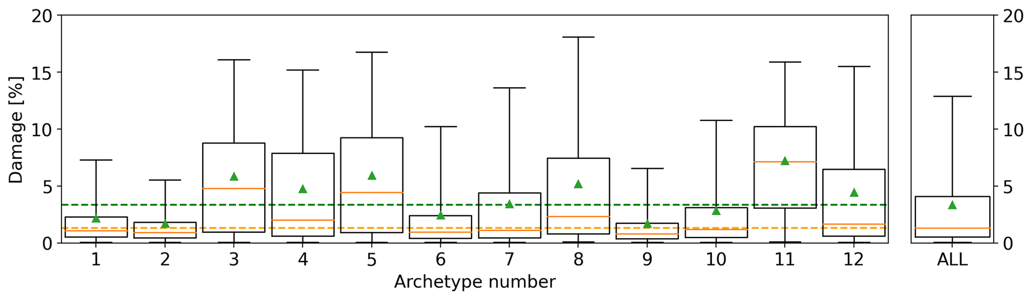
Figure 1Relative damage distribution for each archetype. The black box shows the extent of the 25th and 75th percentiles of the data; the orange line shows the median and the green triangle the mean. The whiskers show the 5th and 95th percentiles. The dashed green and orange lines show the mean and median of the full dataset, respectively.
2.2 Event identification
Insurance data were limited to hail damage claims but the percentage of days with claims in most radar domains did not accurately represent the true hail frequency, with most days recording at least one claim. The majority of these days recorded fewer than 10 claims each, while a small number of days saw claim spikes in the thousands (Fig. 2). To address this issue, we defined intense hail events as days with at least 1000 claims, and days with between 500 and 999 claims were classified as medium hail events. A close look at the days surrounding these events show increased claim counts above the baseline starting around 1 week before and returning to baseline about 1 week after the peak, potentially due to mislabeling of the date or errors in the reported date of damage. To mitigate this, claims within ±7 d from each peak were included in the event's dataset.
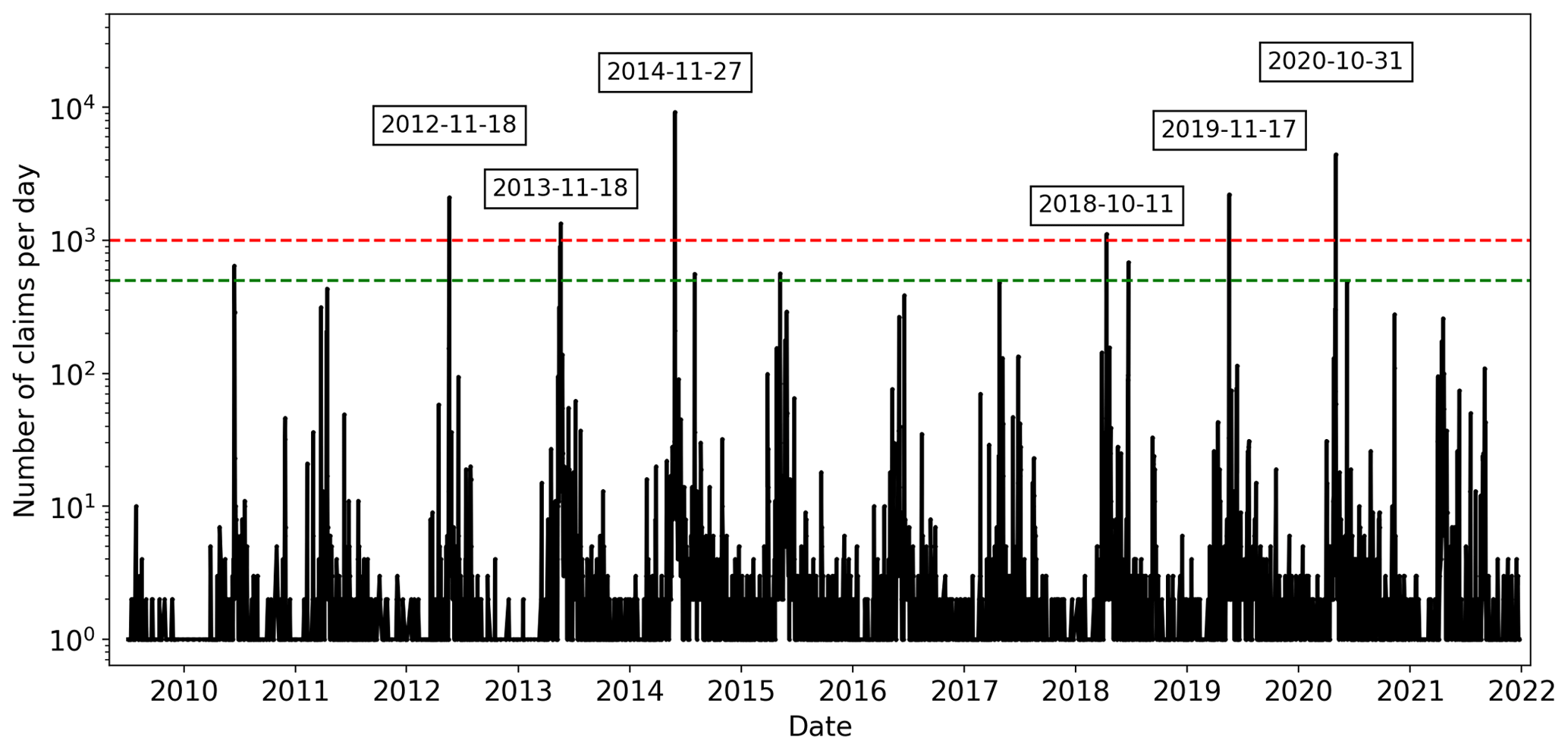
Figure 2Time series of daily claims for the Brisbane radar domain (Mt. Stapylton). Events with more than 999 claims are labeled. A maximum distance of 150 km to the radar was used. The dashed green and red lines show the 500 and 1000 thresholds, respectively.
2.3 Claim filtering
To ensure that only regions with sufficient exposure and a substantial number of damaged properties were included in the analysis, we applied several filters to the insurance dataset.
- 1.
Exposure filter. Policies were considered valid during an event only if at least 10 other policies were also valid within a 1 km radius of the policy in question. This filter helped eliminate areas with insufficient exposure.
- 2.
Damage filter. Damage claims were retained only if they were associated with regions where at least 5 % of policies within a 1 km radius reported damage. Otherwise, these claims were excluded. This filter aimed to identify areas with substantial damage.
- 3.
No-damage filter. If a policy did not report damage, it was removed from our analysis if more than 1 % of neighboring policies (within a 1 km radius) reported damage. This step ensured that areas with less than 1 % of properties reporting damage were classified as “no-damage” areas. One of the reasons to exclude properties without damage within an area with significant damage is because hail fall can only be a small portion of a 1 km square grid; including undamaged properties would artificially lower the actual damage created by hail when averaged. We do recognize that this method might prevent the identification of certain properties that, due to their low vulnerability, do not record damage even when exposed to hail.
The difference between the two percentage thresholds (≥5 % for damage areas and ≤1 % for undamaged areas) created a “buffer zone” where the occurrence of hail damage was considered uncertain. Once these filters were applied, the insurance data were gridded to match the radars' grid for each domain precisely. This involved calculating the mean damage within the boundaries of each radars' grid box. It is important to note that grid points with mean damage above zero only represent damage claims, as undamaged policies were removed from these areas. These filtering thresholds were determined empirically and were found to have a minimal impact on the analysis when varied by up to 10 %. Figure 3 provides a visual representation of the effect of this filtering and the subsequent gridding. After applying all the filters, our dataset consisted of 18 intense hail events and 12 medium hail events; these provided 1775 damage grid points and 76 703 exposed but undamaged grid points. On average, the filtering process removed approximately 21.4 % of damage claims and 12.3 % of exposed but undamaged policies.
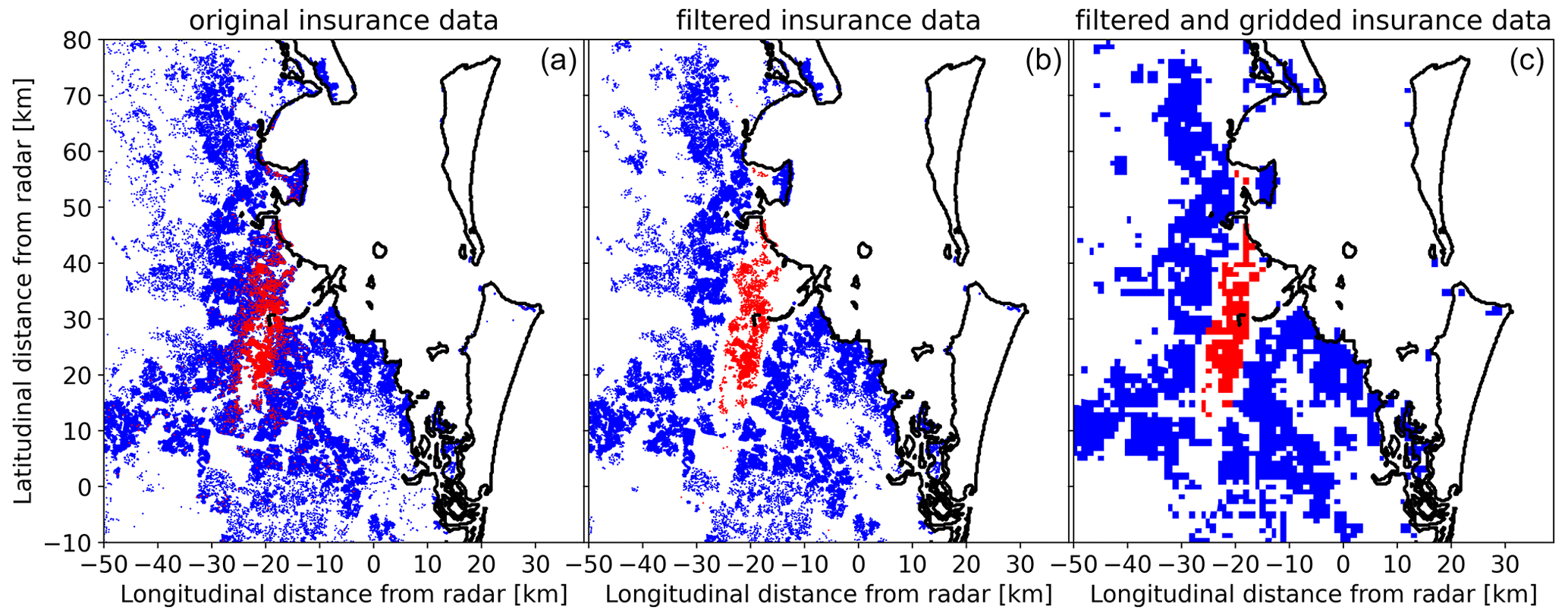
Figure 3Effect of filtering insurance data; red points show valid policies with reported damage, blue dots show valid policies with no reported damage, and white spaces show no valid policies. Panel (a) shows the raw data, panel (b) shows only policies after filtering, and panel (c) shows the gridded filtered data for the event.
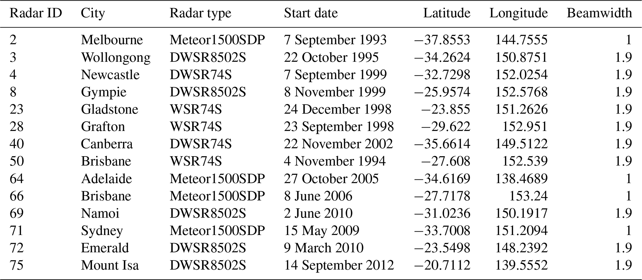
In this study, data from the bureau's radar network were utilized (Soderholm et al., 2022), with a focus on selecting S-band radars that are better suited for hail observations compared to C-band radars (Ryzhkov et al., 2013). Although this led to a reduction in the number of radar sites used in the analysis, it still covered a large proportion of the population and claims. The geographical distribution of these radars can be observed in Fig. 4, and configuration details can be found in Table 1. Note that only the S-band radars in solid blue circles in Fig. 4 were used in relation to the insurance claims as the other S-band radars (dashed lines) did not record hail events within their domains, or their domains were already covered by other S-band radars. Nevertheless, these other S-band radars, in dashed circles in Fig. 4, are used later in the study in the subsection “HDE–MESH relationship” and in Sect. 6. The radar reflectivity was calibrated following the method outlined in Louf et al. (2019) and gridded at a 1 km horizontal and 500 m vertical resolution. The methodology described in Dahl et al. (2019) (Appendix A) was implemented, which uses linear interpolation in elevation and radius of influence on the azimuth range space. Grid points too far from (>150 km) or too close to (<6 km) the radar site were excluded from the dataset.
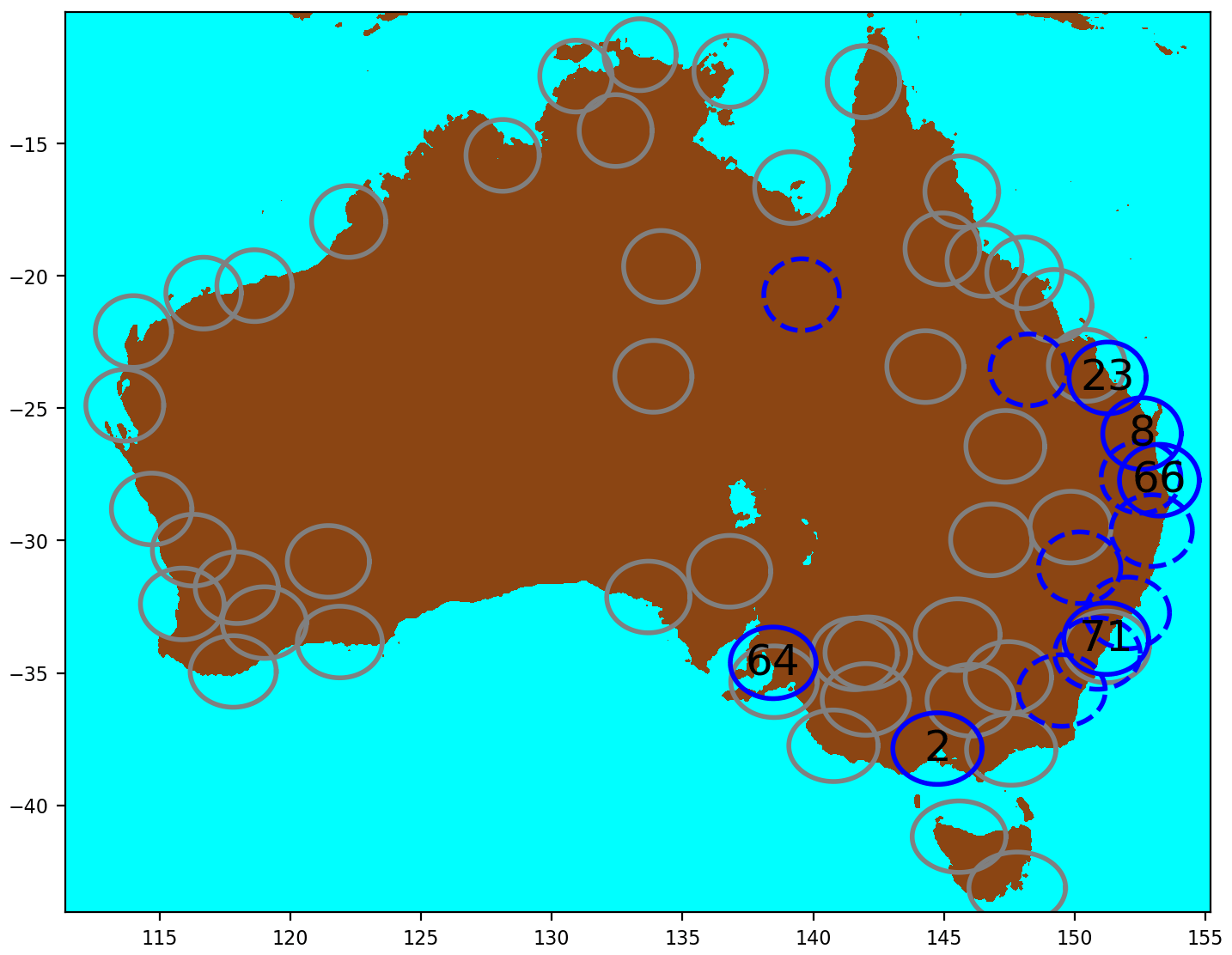
Figure 4Map of the bureau's full radar network. The circles represent the coverage of each radar, with numbers corresponding to the radar ID as listed in Table 1. C-band radars are shown in grey and S-band radars are blue, with solid blue circles indicating the radars used in conjunction with insurance claims. The dashed S-band radars recorded no hail events occurring within their domains and were not used in most of the study except Sects. 6 and 5.3, as these do not involve claims.
3.1 Severe hail index (SHI)
The SHI quantifies hail severity using a weighted vertical integration of reflectivities above the environmental freezing level (Witt et al., 1998). The resulting output is a 2D gridded map which is indicative of the severity of the hail event. In order to calculate SHI, knowledge of the height of the 0 and −20 ∘C dry bulb levels is needed, as the integration of reflectivities is done only between these heights. This information about the temperature profile was retrieved from ERA5 (Hersbach et al., 2020) from the grid point closest in time to the observation and location to the radar location.
3.2 Maximum estimated size of hail (MESH)
The maximum estimated size of hail (MESH) is a quantitative tool that transforms SHI into hail size by fitting SHI to a chosen percentile of maximum observed hail size by using a power curve originally developed by Witt et al. (1998) and improved by Murillo and Homeyer (2019) with a larger report dataset. For this study we use the 75th fit for the Murillo and Homeyer (2019) dataset. This transformation enables the estimation of hail size from the SHI data.
3.3 Calculation of event SHI swath
The event SHI was computed for each grid point within a radar's coverage for the event's day ±1 d to account for possible discrepancies between the reporting time of damage, which has at most a daily accuracy, and the time of radar observations. This extra day on both sides of the event's date prevents missing part of the hailstorm swath when it spans 2 different days. For example, a storm could start on Sunday, 2 h before the end of the day, and last 8 h in total. In such a scenario most claims will likely be assigned to the following Monday. If only Monday's radar data are used, the first 2 h of the swath would be missing from the SHI swath. Since the maximum SHI for each grid point is being taken and no two events occur one after the other in the dataset, the addition of the 2 extra days has no detrimental effect but solves any of the aforementioned timing issues. This computation enabled the production of a storm swath map for each event day (Fig. 5). The volume scan period for radars used in this study ranges from 5 to 10 min, leading to discontinuous SHI swaths, which are most pronounced for fast-moving storms (Fig. 5a). To mitigate this spurious discontinuity, an interpolation algorithm was employed, which uses the estimated field advection from its optical flow to fill in these gaps (Fig. 5b). This is done using the SciPy Python package, specifically the minimize method of the optimize class, which applies the Nelder–Mead minimization algorithm (Nelder and Mead, 1965). This algorithm compares two subsequent scans (images) and attempts to minimize the difference between the two images by displacing one and comparing to the other. Once the optimal displacement is computed, a linear interpolation between the two time stamps is calculated. Once the interpolation between scans is computed, the maximum SHI for each grid point is retained from the two original time stamps and the interpolation, along with its corresponding time stamp, allowing for the retrieval of the associated meteorological conditions from ERA5.
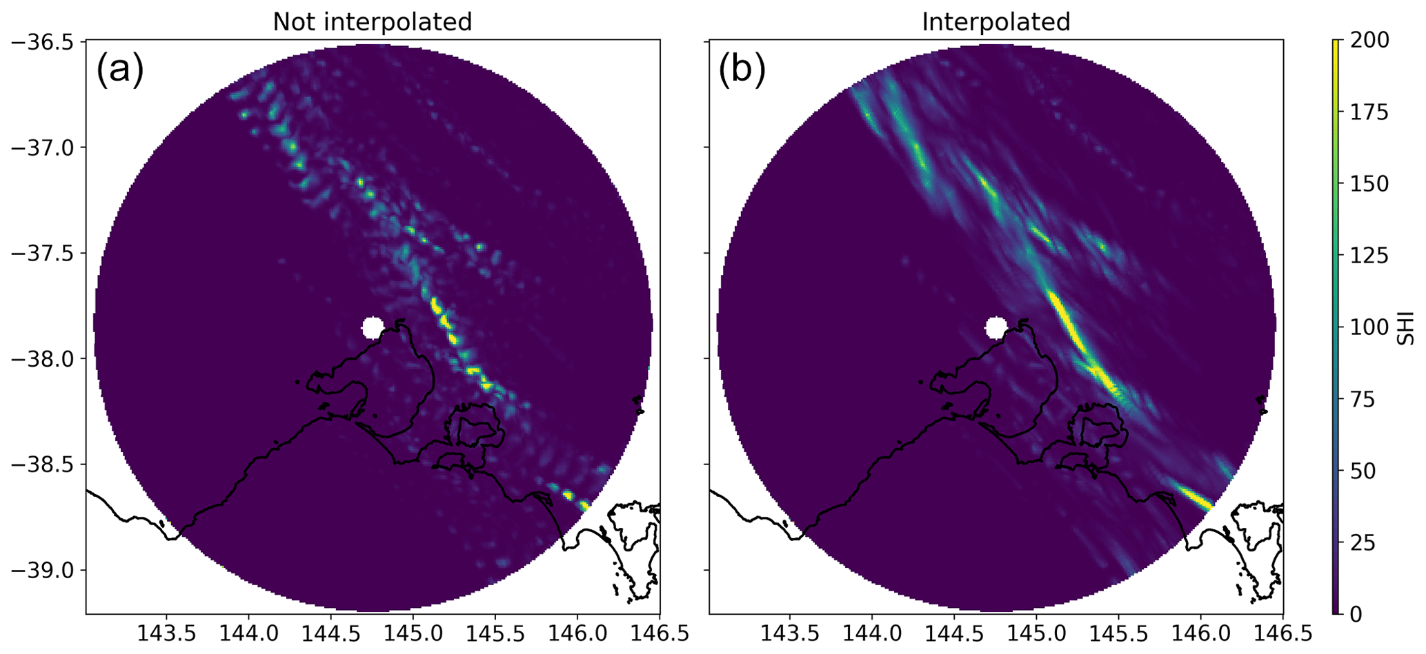
Figure 5Severe hail index (SHI) daily maximum for a sample event. Panel (a) shows a discontinuous storm track due to the time gap between successive radar scans. Panel (b) shows the same day with interpolated data based on the optical flow of SHI.
3.4 Associated meteorological data
Meteorological variables were extracted from ERA5 at ground level and freezing height, including 3D wind components, specific humidity, divergence, vorticity, atmospheric temperature, and atmospheric pressure. CAPE and CIN (most unstable convective available potential energy and convective inhibition, respectively), were also extracted; for more details on the calculation of these variables see Groenemeijer et al. (2019). All these variables were retrieved for each grid point at the time when the maximum SHI of the day occurred. These data served as the input for training the neural network in addition to SHI and the observed damage.
Hail retrievals from radar observations aloft often do not align with observations at ground level, resulting in a common mismatch (Brook et al., 2021). MESH and SHI are calculated from reflectivities above the environmental freezing level, which can reside several kilometers above the surface. Depending on the strength of storm-generated and environmental winds, hail descending below this level may be advected several kilometers from its initial location, leading to the aforementioned mismatch. By design, MESH (and, by extension, SHI) would have greater skill as a predictor of hail damage during events where hail falls with little horizontal movement. To address this issue, we developed a virtual advection (VA) algorithm, which matches ground-level observations of hail damage to the appropriate radar observations aloft, mitigating this error. Similar approaches have produced substantial improvement of the correlation between observed damage and radar-derived hail estimates (Schiesser, 1990; Hohl et al., 2002; Schmid et al., 1992; Schuster et al., 2006).
4.1 VA algorithm and assumptions
To apply the VA algorithm, we made certain assumptions. We assumed that the highest damage within a local area corresponded to the highest observed SHI values aloft, given that differences in vulnerabilities of properties is already mitigated by the archetype normalization. However, this assumption may not hold true in cases in which the hailstorm area is not densely covered by insured properties, and large hailstones may fall in uninsured areas or areas without buildings. In such cases, this assumption would systematically lead to a positive bias in SHI values. To address this issue, we filtered the claim data to only include grids with sufficient exposure, as described in Sect. 2.3. To match damage to SHI, we first sorted each event's normalized gridded damage dataset in descending order according to value. Then, we matched the first (highest) damage grid point to the highest SHI grid point within a 4 km radius of influence (RoI) around the damage grid point. Once we established a pair of damage and SHI grid points, we stored the pair in a new VA dataset with its associated horizontal displacement vector and meteorological variables (from ERA5). We removed this SHI grid point from the available SHI grid and repeated the process until we matched all damage grid points to SHI observations. Once there were no more damage grids, the average horizontal displacement vector was calculated. The matching was restarted but with the average horizontal displacement vector already applied to the 4 km RoI. This double-pass approach allowed correcting for the environmental wind displacement (represented by the average horizontal displacement vector of the first run) and the storm-generated winds (done in the second run). The 4 km RoI was selected empirically, with higher values showing only small improvement in the relationship between SHI and damage and smaller numbers showing poor visual matching of the radar and damage swaths. When both runs were used, up to 8 km of displacement can be achieved, as both runs could result in displacements in the same direction for a given claim–SHI grid pair. However, this was rare for the studied events, with most events having an average final displacement (after the second run) less than 2 km and none of the events having average final displacements above 4 km. Note that no local consistency in the displacement vector is enforced for the second run, which allows convergence and divergence of the SHI field. If all nonzero SHI observations are used before matching all damage grid points, then the closest zero SHI observation is used within the RoI. For grid points with contracts and zero observed damage, we matched the lowest SHI observations (including zero) within the RoI instead of the highest. Grid points with no valid SHI observations within the RoI due to being too far from or too close to the radar site were excluded from the VA dataset.
We assessed the performance of the VA algorithm using the 2014 Brisbane hailstorm, a well-known event with substantial advection that resulted in a large mismatch between MESH (SHI) observations and reported damage locations (Brook et al., 2021; Warren et al., 2020). Figure 6a shows this mismatch. To visualize the algorithm's performance, we calculated the weighted average (by damage) of the horizontal VA displacement vectors (yellow star in Fig. 6c). We then displaced the original MESH grid by this average vector (Fig. 6b), resulting in much better agreement with the observed damage. We refer to this displacement by the average vector as bulk-advected to differentiate it from the data produced by the VA algorithm, which are visualized in the 2D histogram of Fig. 6 (panel c). When comparing this bulk advection with the Brook et al. (2022) individual modeling of the hailstone trajectories for this event, good agreement can be observed for the overall swath displacement. In addition, Brook et al. (2022) found that the average motion vector for this event was 2.1 km in a northwesterly cardinal direction, which is very similar to our aforementioned weighted average horizontal displacement (2D histogram in Fig. 6).
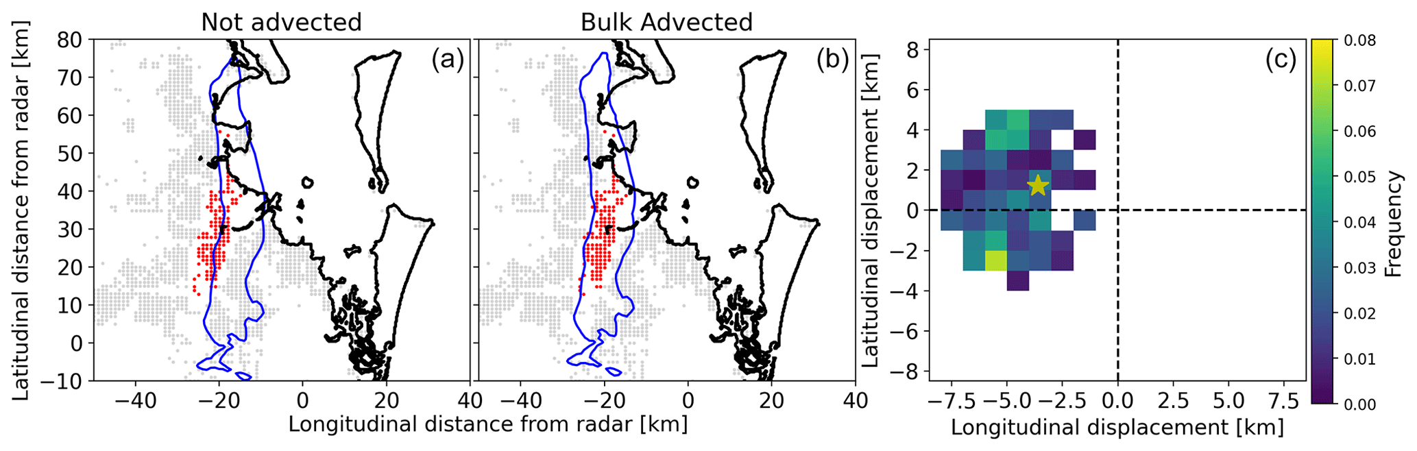
Figure 6Sample of virtual advection of a severe hail event (Brisbane 2014). Panel (a) shows grid points with exposure that reported no damage in grey, damaged grid points in red, and grid points with insufficient exposure in white. The blue contour line is derived from MESH at 40 mm. Panel (b) shows the same but with MESH displaced by the weighted average (by damage) of the virtually advected data. Panel (c) shows the histogram of the horizontal displacement of MESH to match the damage at ground level, and the yellow star shows the weighted average.
4.2 Performance comparison
The VA algorithm was applied to all hail events, and the resulting MESH–damage dataset is presented in Fig. 7a. Figure 7b shows the performance diagram (Roebber, 2009) for various MESH thresholds above which damage is predicted for each advection correction type. Here the 40 mm threshold shows the highest critical success index (CSI) for all correction types; this threshold is shown in panel (a) (dashed green line), revealing that most damage occurs for MESH values above this threshold. This diagram illustrates clear improvement for the advection-corrected sets, with the VA algorithm substantially outperforming the bulk advection method. The scatter plot in this panel highlights two events in blue and red that exhibit distinct MESH–damage relationships. Note that since the contours of individually advected MESH are not well defined for non-damaging hail and the relationship between the radar hail estimate and observed damage is poor for the bulk-advected dataset, maps of radar-derived hail products for all following sections are bulk-advected, while scatter plots comparing these products to damage are individually advected.
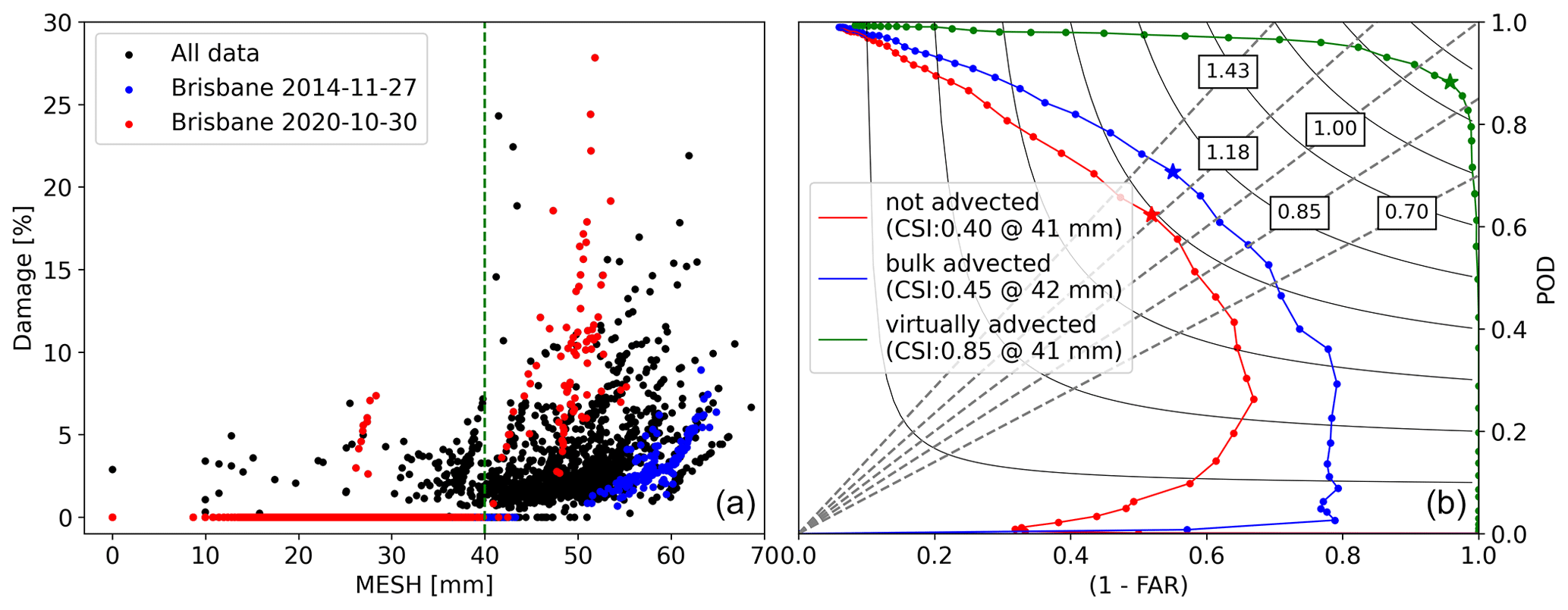
Figure 7Relationship between MESH and damage. Panel (a) shows virtually advected MESH against observed damage, with the dashed green line showing the best CSI threshold (for all correction types). Panel (b) shows the Roebber performance diagram for non-advected MESH, bulk-advected MESH, and individually (virtually) advected MESH. The stars in the right panel show the best CSI for each dataset. The dashed grey lines show the bias with their respective values in boxes.
In this section, we explore the limitations of using MESH as a predictor of hail damage intensity and present a novel approach for estimating hail damage. While the VA algorithm improves the performance of MESH as a hail damage predictor when above 40 mm, its ability to estimate damage intensity remains inconsistent across different events, as demonstrated in Fig. 7a. This inconsistency suggests that the relationship between MESH and hail damage intensity is dependent on other factors specific to each event, such as the meteorological condition conducive for hail growth, since differences in vulnerabilities due to property factors have already been mitigated (see Sect. 2.1). Furthermore, radar reflectivity has inherent limitations since radar reflectivity is the integral of the particle size distribution times the diameter to the sixth power under the Rayleigh approximation, so the same reflectivity could be produced by either a few large hailstones or a high concentration of smaller hailstones, which would result in very different severity of hail damage for the same reflectivity (and therefore SHI). In addition, the presence of other hydrometeors like ice crystals or liquid water can further decouple observed reflectivity from severity of hail damage. To explore the information content of meteorological conditions for improving hail damage estimate, we developed an artificial neural network that incorporates meteorological variables associated with each grid point to improve the SHI–damage relationship. Our approach generates hail damage estimates (HDEs) that demonstrate better agreement with the observed damage.
5.1 Neural network structure and selection of input variables
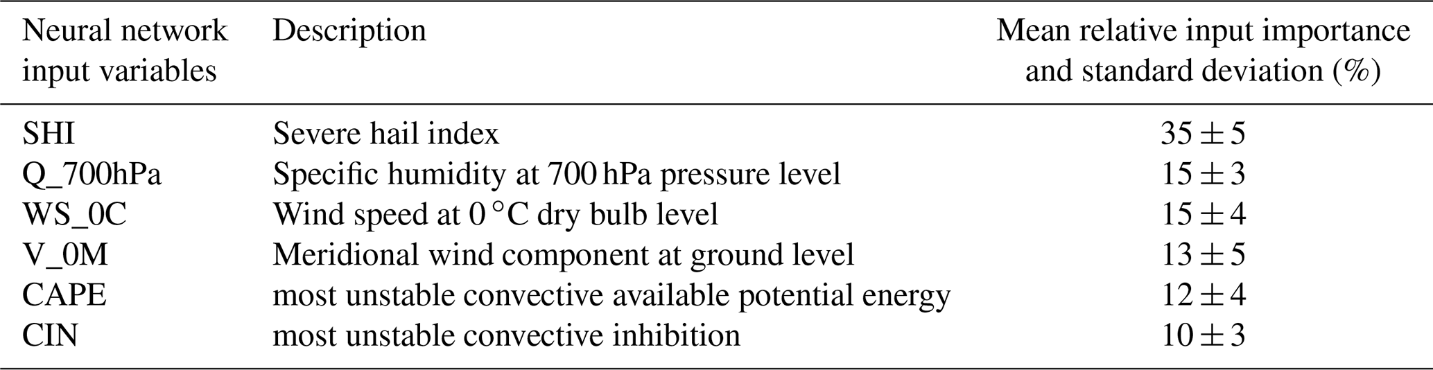
To develop and train the HDE neural network, we utilized TensorFlow and Keras (Abadi et al., 2015). Initially, a wide range of meteorological variables and radar products were incorporated into the model. We then applied the Shapley additive explanations (SHAP, Lundberg and Lee, 2017) analysis to identify the most skillful variables, i.e., those with the greatest impact on the prediction (Table 2). This allowed us to maintain the model's accuracy while minimizing its complexity. While initially the network was deeper, it was optimized to maintain accuracy while minimizing computational cost; our final configuration consisted of six layers, each containing 6 (input), 9, 7, 6, 3, and 1 (output) neurons, all of which were densely connected and activated using a rectified linear activation function (excluding the output neuron, which was linear). We linearly normalized the input variables to ensure their values ranged between 0 and 1.
Table 2Variables used as input for the hail damage estimate (HDE) and their relative importance.
5.2 Training and performance
To train our model, we utilized the VA dataset, which contained the 18 intense and 12 medium hail events. We had access to 78 486 distinct damage–SHI points that matched our criteria, with 37 145 points indicating no reported damage and zero SHI, 39 558 indicating no damage but SHI > zero, and 1775 indicating both reported damage and SHI above zero. Due to the highly unbalanced nature of the data (i.e., no damage greatly outnumbers damage), we set the model's initial bias to the natural logarithm of the ratio between the damage count and the no-damage count (−3.762). By setting the initial bias to the logarithm of the class ratio, we are effectively providing the model with a starting point that takes into account the class imbalance (He and Garcia, 2009). We randomly separated the data into two groups: a training dataset (80 %) and a validation dataset (20 %). To avoid the training and validation dataset being highly correlated, the separation was done event-wise, meaning that six random events were used as validation and the other 24 as training. The meteorological data associated with nonzero SHI points are well defined, as the time when this SHI occurred is known. This is not the case when a grid point with zero SHI (i.e., outside the storm swath) and any time and therefore associated meteorological data can be assigned. To ensure that the meteorological data used for training were representative of both hail and non-hail atmospheric conditions, we selected random time stamps within ±1 d of the event for grid points where the SHI was zero. We trained the model 1000 times for 1000 epochs each, with random separation of the two sets (24 training events and six validation events) and randomly initialized model weights but with the same initial bias. Figure 8a displays a representative training time series, demonstrating that the trained model performs well on the training and validation datasets. The vertical dashed line in this panel indicates the epoch when the model reached its optimal training state, before overfitting, and this weight set was then applied for that specific training attempt. To calculate HDE, we utilized an ensemble approach with seven members (from the 1000 random training attempts) that maximized CSI and the coefficient of determination (R2). This number of members showed the best balance between computational cost and performance, with additional members showing minimal improvement on the ensemble's skill. The resulting ensemble mean yielded a CSI of 0.88 and an R2 of 0.79 compared to observations for the full dataset, the 18 intense hail events, and 12 medium events. However, the model tends to underestimate large damage (> 10 %), as depicted in Fig. 8b; this is likely due to the under-representation of such cases in the dataset. It is important to note that this CSI was achieved at a 0.5 % damage threshold. From the observed damage data (see Figs. 7, 8, and 9), it is evident that there are only a few claims between 0 % and approximately 0.5 %. This is likely because losses below this ratio fall below the policies' deductibles and, therefore, are often not reported by property owners. This apparent discontinuity in the observed damage data was also observed in the unfiltered data (Sect. 2.3), indicating that it is not a result of the elimination of uncertain damage areas.
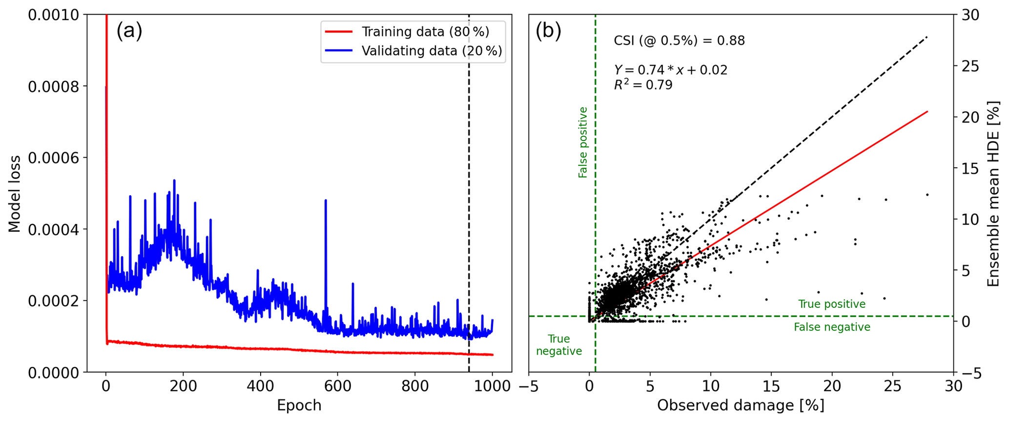
Figure 8Panel (a) shows a sample training time series of the model's loss for the training and validation data, with the dashed vertical line showing the epoch when the model reached the optimal training state before overfitting. Panel (b) shows the relationship between observed damage and the HDE ensemble mean. CSI is calculated based on a 0.5 % damage threshold (dashed green lines). The red line shows the best fit with its equation and coefficient of determination shown on the top left corner. The dashed black line shows the 1:1 relationship.
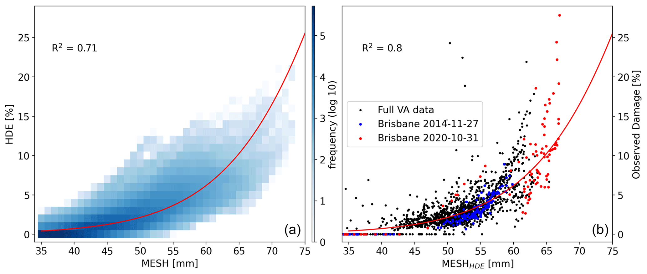
Figure 9Panel (a) shows HDE and MESH calculated for the full radar archive as a 2D histogram with 1 % and 1 mm bins with the best fit of Eq. (1). Panel (b) shows the relationship between observed damage and MESHHDE, with the previously highlighted events shown in red and blue.
5.3 HDE–MESH relationship
To understand the relationship between HDE and the conventional MESH retrieval, a much larger HDE dataset was required than that available from the VA dataset. Therefore HDE and MESH were calculated for all S-band radars of the Australian operational weather radar archive. In Fig. 9, we present the data obtained. A sigmoid function (Eq. 1) provided the best fit for the data while representing a physically realistic relationship, where damage asymptotically approaches 100 % as MESH tends to infinity.
This type of relationship has been used before to relate radar-derived hail estimates to hail damage (Schiesser, 1990). Only points where MESH >35 mm are shown, as the remaining data points were too numerous to display and damage tends to zero. The fit is relatively good (R2=0.71), indicating a reasonable correlation between MESH and HDE. Using the inverse of Eq. (1), we calculated MESHHDE, which allows for an investigation of how the neural network adjusts the radar observations (SHI) using the environmental information. Note that MESHHDE is not intended to replace MESH as a reliable size of hail, but rather as a tool to identify where the model has decreased or increased hail intensity according to the environmental conditions.
We then examined the relationship between MESHHDE and observed claims for the events captured by the damage dataset, as shown in Fig. 9b, with the two Brisbane events previously highlighted in the same colors. The relationship is greatly improved, and both events now show more consistent sizes relative to the observed damage.
5.4 HDE case studies
In this section we show the performance and behavior of HDE for the two previously highlighted hail events to analyze how different meteorological conditions drive HDE behavior.
5.4.1 Brisbane 2014 hail event
On 27 November 2014, Brisbane experienced a severe hailstorm that caused substantial damage to a densely populated area, resulting in over AUD 1.5×10⁹ losses (normalized to 2017) and more than 9000 individual building claims (for Suncorp). Giant hailstones, reportedly measuring around 70 mm in size, were observed during this event (Parackal et al., 2015). In Fig. 10, we present MESH and MESHHDE for this event. We observed that MESHHDE assigns low values of MESH to zero due to the inability of low MESH values to cause any damage to property, therefore resulting in zero HDE. Additionally, within the easternmost storm cell, where MESH is high and damage occurred, MESHHDE was mostly lower than MESH, as highlighted in panel (f). This finding shows that MESHHDE more closely aligns with the mean fit (dashed green line in panel f) and corrects the observed positive bias of this event when compared with the original VA data. While MESHHDE shows a more consistent fit, it is evident that it is not a good representation of the actual size of expected hail as it is still far below the observed size for this storm. Panels (d) and (e) show the MESH and MESHHDE contours over the observed damage, respectively.
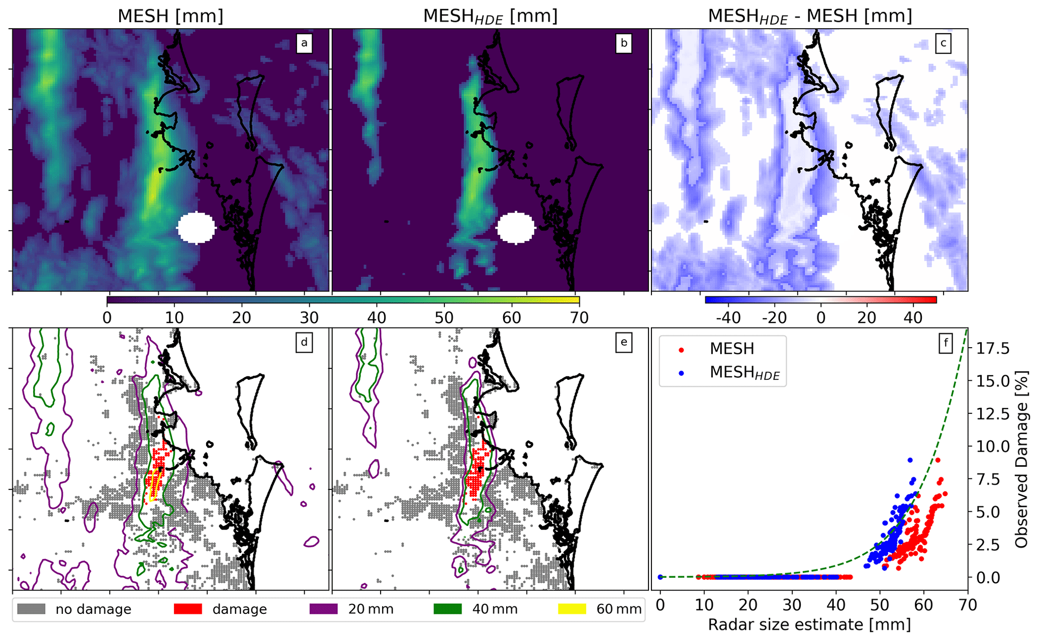
Figure 10Comparison of MESH, MESHHDE, and observed damage for an intense hail event in Brisbane on 27 November 2014. Panels (a), (b), and (c) show maps of MESH, MESHHDE (MESH derived from HDE), and the difference between the two, respectively. Panels (d) and (e) show observed damage with bulk-advected MESH and MESHHDE contours overlaid. Panel (f) shows the relationship between observed damage and the grid-point-advected MESH and MESHHDE.
5.4.2 Brisbane 2020 hail event
In contrast to the 2014 event, the 2020 Brisbane hail event showed a negative bias in MESH relative to the full VA dataset. As shown in Fig. 11, MESHHDE was lower than MESH for most of the domain but considerably higher than MESH where hail damage occurred. It is worth noting that this case exhibited some potentially spurious claims, as highlighted within the red circles in the panel (f). All these points were tracked and found in a cluster in the map (indicated by the red circle in the panel e) close to the coast. They were relatively far from the main storm swaths and could be due to the misclassification of damage cause (i.e., wind or flood damage instead of hail) in the insurance dataset.
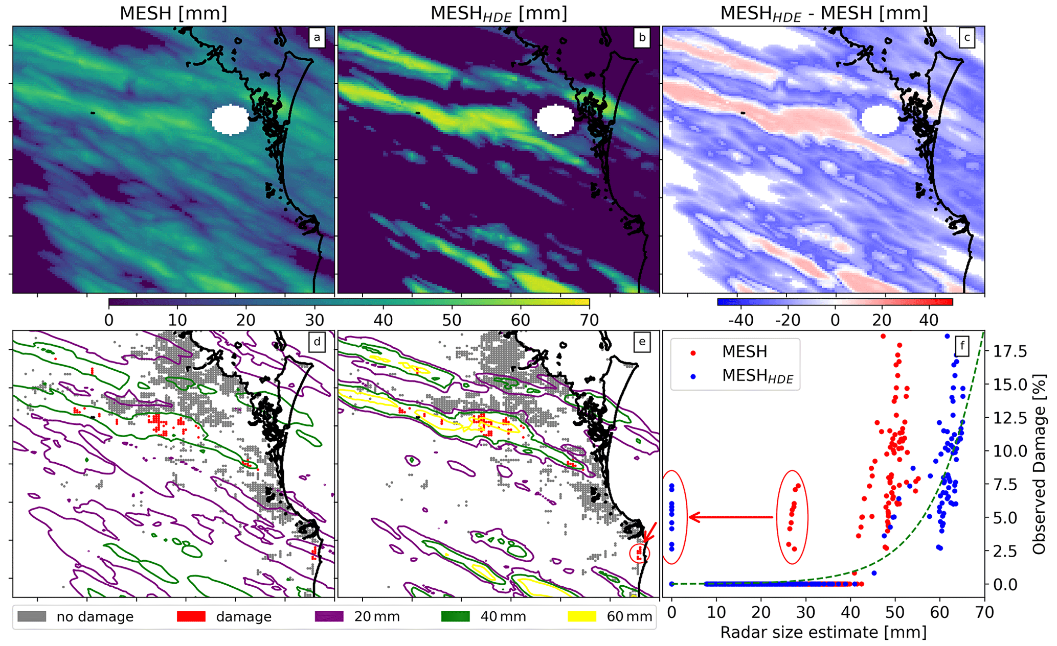
Figure 11Same as Fig. 10 but for an intense hail event in Brisbane during 31 October 2020. The red circles in panel (f) show potential spurious claims; these were tracked to the map and are shown in panel (e) within a red circle.
The 2020 event was associated with very different meteorological conditions in the ERA5 reanalysis than the 2014 event, with higher CAPE and lower CIN, stronger northerly winds at ground level, lower humidity aloft, and increased winds at the melting layer (Table 3). Looking at the MESH values from these events alone, one would expect the 2014 event to have caused more damage than the 2020 event, as the mean MESH values in the storm cores (here defined as the areas with HDE above zero) were 58.3 and 51.6 mm, respectively. Nevertheless, in the observed damage dataset, the 2014 event produced lower damage than the 2020 event, as is clearly visible in Fig. 7. This discrepancy is not observed in MESHHDE, with mean values of 51.3 and 61.4 mm for the 2014 and 2020 events, respectively.
Table 3Mean values of MESH, MESHHDE, and environmental parameters for storm cores during the 2014 and 2020 Brisbane events. The error bounds show the standard deviation within the storm cores.

The cases mentioned highlight the possibility of storms with relatively low MESH values causing severe damage, such as the one that hit Brisbane in 2020, or relatively high MESH values leading to comparatively lower damage, as seen in the 2014 Brisbane storm. The disparity could be attributed to a mixture of hail and other hydrometeor types (liquid water, ice crystals), which would result in a higher MESH value than a volume containing only the hail component. Further, MESH uses the environmental freezing level, but the updraft's freezing level could be well above the environmental freezing level, which could involve larger liquid water droplets than conventional supercooled liquid water droplets (Kumjian and Ryzhkov, 2008). The disparity could also be attributed to differences in the HSD in these volumes. Volumes with different HSD but equivalent scattering response would produce similar MESH values but varying ground damage. Since supercooled liquid water (SLW) droplets are considerably small, most of the reflectivity signal is expected to be caused by hail, smaller frozen hydrometeors, or large liquid water droplets lofted above the environmental melting layer.
Extending this method, we can utilize the difference between MESHHDE and MESH (hereafter ΔMESH) as an indicator of the skewness of the HSD within a storm, differences in hail hardness, and/or mix hydrometeor volumes. Positive ΔMESH indicates a larger proportion of damaging hailstones, harder and/or denser hailstones, and/or a lower proportion of mixed hydrometeors in the volume, while negative ΔMESH indicates the contrary.
Figure 12 shows the relationship between each meteorological parameter and HDE as well as ΔMESH as box plots for the full radar archive. Using 40 mm for MESH and 0.5 % for HDE as thresholds for damage and HDE as the truth, the leftmost column (panels a, e, i, m, and q) represents environments where MESH indicates a false positive for hail damage, while the second column (panels b, f, j, n, and r) shows opposite environments, where MESH indicates a false negative. The Kolmogorov–Smirnov (Hodges, 1958) test was applied to each meteorological variable for the false-positive and false-negative cases, showing that while all sets showed significant differences (p values approaching zero), specific humidity aloft showed a substantial difference between the two cases, with D-statistics of 0.64, which is evident from the corresponding box plots. A clear threshold was identified based on the analysis (dashed horizontal line in panels a, b, c, and d). It was found that 82 % of the false-positive occurrences happened in environments where the specific humidity at 700 hPa was above 0.0053 kg kg−1. Coincidentally, the same percentage of false-negative occurrences happened in environments where the specific humidity at 700 hPa was below that humidity threshold. By utilizing this threshold and applying it only for MESH values between 39 and 41 mm, which account for approximately 50 % of the false-positive and false-negative cases, the CSI of MESH can be improved from 0.76 (at 40 mm against HDE) to 0.79. Environments with false-positive results exhibited conditions similar to those in negative ΔMESH bins and low-HDE bins. This indicates that most of these false positives resemble environments associated with negative values of ΔMESH and are less likely to have high HDE. False-negative cases were associated with low HDE and showed similarities to environments with a positive ΔMESH bias, and these cases had an average HDE of 0.8 % and a maximum of 4.2 %. CAPE tends to increase with ΔMESH, whereas CIN is larger for more extreme ΔMESH of either sign. Looking at the relationship to winds, there is a positive correlation with ΔMESH, except for the extreme positive end. In a similar way these extreme values of ΔMESH are associated with northward winds at the ground compared to the rest of the distribution that exhibits no trend.
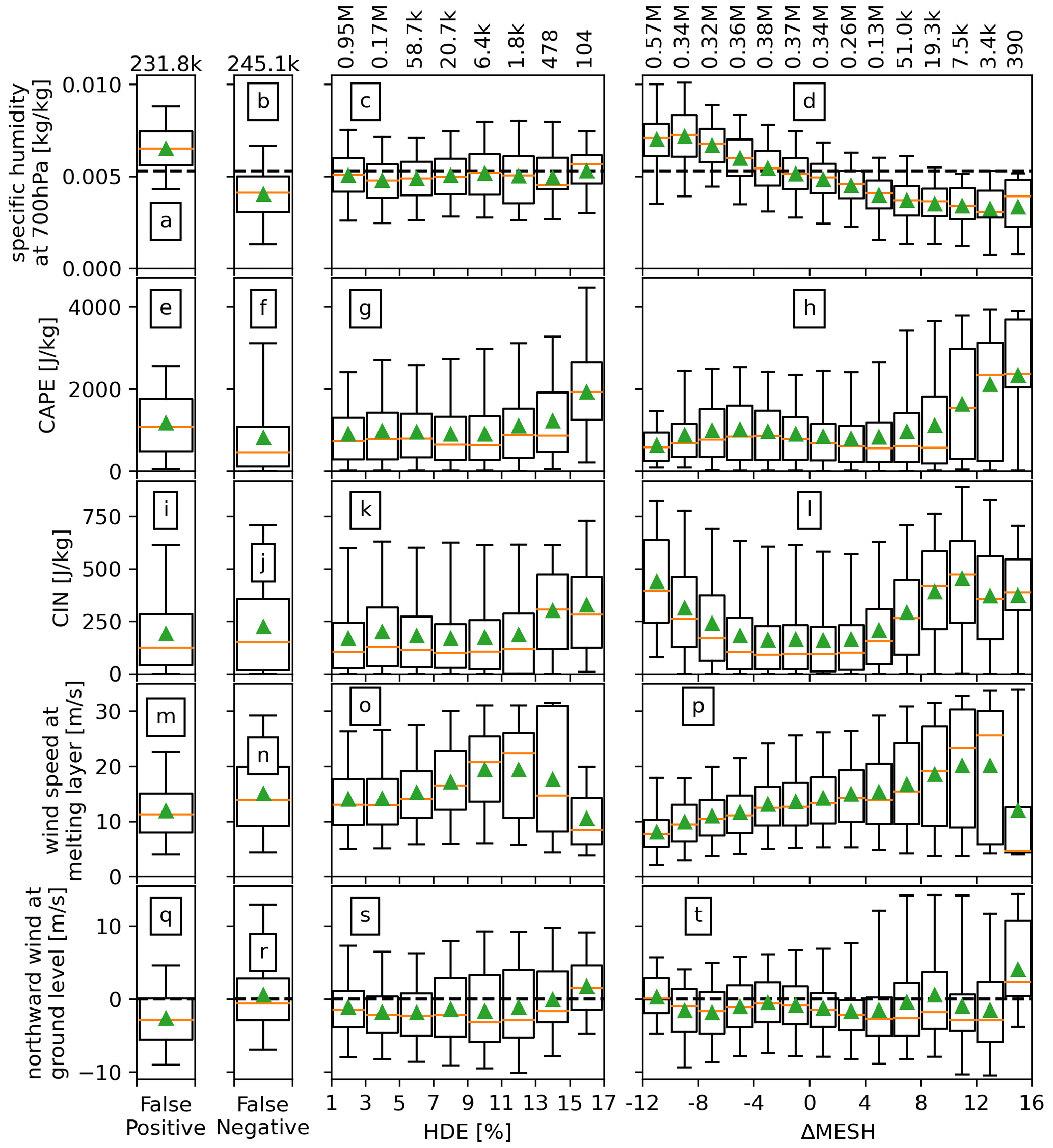
Figure 12Box plots of the meteorological variables that drive the HDE model. From left to right columns: (first) for HDE <0.5 % and MESH ≥40 mm; (second) for HDE ≥0.5 % and MESH <40 mm; (third) for HDE ≥0.5 % in 2 % bins; (fourth) for HDE ≥0.5 % in 2 mm bins. The third and fourth columns show the distribution as a function of HDE and ΔMESH, respectively. Sample sizes per bin are shown on top. The box plots follow the same style and structure as Fig. 1, top panel.
This analysis indicates that environments with relatively low specific humidity, high CAPE and CIN, low wind speeds aloft, and northward winds at the ground are likely to have HSD with a higher proportion of large hailstones or a lower proportion of other hydrometeors. Regarding environments associated with extreme values of hail damage, these are associated with high CAPE and CIN values, lower wind speeds at the melting layer, and northward winds at the ground. No clear signal with respect to specific humidity aloft is observed. A recent modeling study on hail production (Lin and Kumjian, 2022) found that CAPE acts as a modulator to hail growth, with a non-monotonic relationship with hail size which peaks around 2000–2400 J kg−1. Although we do observe that about 50 % of the samples with high values of HDE occur close to this CAPE range (Fig. 12g), these HDE bins also show about 25 % of samples with CAPE values above 3000 J kg−1 and a clear positive correlation between CAPE and HDE. Regarding the aforementioned HDE relationship with winds, a similar modeling study (Dennis and Kumjian, 2017a) found that increased deep-layer east–west shear increases hailstone mass, while increased low-level north–south shear reduces hailstone mass. Here it is important to note that one of the variables included in the initial input layer of the HDE model was absolute wind speed shear between the surface and the melting layer but was discarded as the SHAP analysis showed that it had low influence on the output relative to the other input variables. The zonal or meridional components of the shear vector were not tested.
This study has analyzed more than 10 years of insurance and radar data from Australia to investigate the performance of the maximum expected size of hail (MESH) retrieval in predicting and quantifying hail damage. The results showed that MESH has poor predictive value for damage magnitude estimation but shows good skill (CSI =0.88 for MESH larger than 40 mm) as a binary predictor of hail damage when corrected for horizontal advection of hailstones, which is consistent with Brook et al. (2021).
To improve damage magnitude estimation, a neural network was trained with meteorological variables from ERA5 in addition to SHI (from which MESH is derived) against observed hail damage. Using SHAP analysis, the most important meteorological variables were identified as specific humidity at 700 hPa, wind speed at the freezing level, northward winds at ground level, CAPE, and CIN. This neural network produced a hail damage estimate (HDE) with high accuracy (CSI =0.88 and an R2=0.78) for estimating hail damage occurrence and intensity.
A comparison of HDE with MESH for the full national radar dataset (14 radars with an average of 18.8 years of coverage) revealed a relatively good (R2=0.71) fit between the two using a sigmoid curve. This curve was used to derive MESHHDE from HDE with the goal of identifying environments where MESH shows negative or positive biases, potentially due to differences in hail size distributions (HSDs) and/or presence of other hydrometeors along with hail.
Environments with negative bias in radar hail estimates are associated with low CAPE, high CIN, and higher specific humidity aloft and are likely to be non-damaging if MESH is below 50 mm. In contrast, environments with positive bias are associated with high CAPE, high CIN, and lower specific humidity aloft and are likely damaging if MESH is above 30 mm. Extreme hail damage was associated with such positive bias environments that in addition showed low wind speeds aloft and northerly winds at the ground.
The study provides important insights into the performance of MESH and SHI for estimating property damage, the potential of using neural networks to improve hail damage estimation, and identifying patterns between environmental conditions and a storm's HSD, hail hardness, and/or presence of mixed hydrometeor precipitation. It is important to note that these results were developed for Australian storm environments and might not be representative of global storm environments. This study was limited to S-band radars, and future work should expand this technique to C-band radars. In addition, future work will explore using this novel hail damage estimate for nowcasting applications to provide hail damage warning. Another limitation to our findings is the relatively small sample of individual storms, which might only sample a subset of all environmental conditions that lead to hail storms. Replicating this work in locations with high population density and radar coverage (i.e., Europe or the USA) would be valuable to potentially mitigate this limitation as well as determine if these same environmental parameters play dominant roles in HDE.
The insurance data provided by Suncorp are not publicly available for privacy reasons. Details regarding the radar data used in this study can be found in the AURA database online at https://doi.org/10.25914/JJWZ-0F13 (Soderholm et al., 2022). ERA5 data can be accessed at https://www.ecmwf.int/en/forecasts/dataset/ecmwf-reanalysis-v5 (Hersbach et al., 2020).
RW and LY prepared the insurance claim data for analysis and contributed to the interpretation and implementation of the archetype normalization. NR validated and tested the HDE product against internal Suncorp models. JS prepared the radar data and SHI–MESH hail estimate products. JS and AP contributed to the development of Sects. 4 and 5 and the interpretation of Sect. 6. LA designed the paper's outline, carried out most of the analysis, and wrote the paper. All co-authors participated in paper-related discussions and commented on the paper.
The contact author has declared that none of the authors has any competing interests.
Publisher's note: Copernicus Publications remains neutral with regard to jurisdictional claims made in the text, published maps, institutional affiliations, or any other geographical representation in this paper. While Copernicus Publications makes every effort to include appropriate place names, the final responsibility lies with the authors.
The authors acknowledge the financial support of Suncorp and the Australian Bureau of Meteorology. We extend our gratitude to Rob Warren and Mark Curtis for their invaluable input and insightful feedback during the internal review process. Their constructive suggestions and edits significantly enhanced the quality of this paper.
This research was funded by Suncorp and the Australian Bureau of Meteorology.
This paper was edited by Yuanjian Yang and reviewed by Tanya Brown-Giammanco and one anonymous referee.
Abadi, M., Agarwal, A., Barham, P., Brevdo, E., Chen, Z., Citro, C., Corrado, G. S., Davis, A., Dean, J., Devin, M., Ghemawat, S., Goodfellow, I., Harp, A., Irving, G., Isard, M., Jia, Y., Jozefowicz, R., Kaiser, L., Kudlur, M., Levenberg, J., Mané, D., Monga, R., Moore, S., Murray, D., Olah, C., Schuster, M., Shlens, J., Steiner, B., Sutskever, I., Talwar, K., Tucker, P., Vanhoucke, V., Vasudevan, V., Viégas, F., Vinyals, O., Warden, P., Wattenberg, M., Wicke, M., Yu, Y., and Zheng, X.: TensorFlow: Large-Scale Machine Learning on Heterogeneous Systems, https://www.tensorflow.org/, 2015. a
Allen, J. T. and Tippett, M. K.: The Characteristics of United States Hail Reports: 1955–2014, E-Journal of Severe Storms Meteorology, 10, 1–31, https://doi.org/10.55599/EJSSM.V10I3.60, 2015. a
Blong, R.: Residential building damage and natural perils: Australian examples and issues, Build. Res. Inf., 32, 379–390, https://doi.org/10.1080/0961321042000221007, 2007. a
Brook, J. P., Protat, A., Soderholm, J., Carlin, J. T., McGowan, H., and Warren, R. A.: HailTrack–Improving Radar-Based Hailfall Estimates by Modeling Hail Trajectories, J. Appl. Meteorol. Clim., 60, 237–254, https://doi.org/10.1175/JAMC-D-20-0087.1, 2021. a, b, c, d
Brook, J. P., Protat, A., Soderholm, J. S., Warren, R. A., and McGowan, H.: A Variational Interpolation Method for Gridding Weather Radar Data, J. Atmos. Ocean. Tech., 39, 1633–1654, https://doi.org/10.1175/JTECH-D-22-0015.1, 2022. a, b
Brown, T. M., Pogorzelski, W. H., and Giammanco, I. M.: Evaluating Hail Damage Using Property Insurance Claims Data, Weather Clim. Soc., 7, 197–210, https://doi.org/10.1175/WCAS-D-15-0011.1, 2015. a
Brown-Giammanco, T. M., Giammanco, I. M., and Estes, H. E.: New Asphalt Shingle Hail Impact Performance Test Protocol and Damage Assessment, Nat. Hazards Rev., 22, 04021050, https://doi.org/10.1061/(ASCE)NH.1527-6996.0000509, 2021. a
Cintineo, J. L., Smith, T. M., Lakshmanan, V., Brooks, H. E., and Ortega, K. L.: An Objective High-Resolution Hail Climatology of the Contiguous United States, Weather Forecast., 27, 1235–1248, https://doi.org/10.1175/WAF-D-11-00151.1, 2012. a
Dahl, N. A., Shapiro, A., Potvin, C. K., Theisen, A., Gebauer, J. G., Schenkman, A. D., and Xue, M.: High-resolution, rapid-scan dual-Doppler retrievals of vertical velocity in a simulated supercell, J. Atmos. Ocean. Tech., 36, 1477–1500, 2019. a
Dennis, E. and Kumjian, M.: The impact of vertical wind shear on hail growth in simulated supercells, J. Atmos. Sci., 74, 641–663, https://doi.org/10.1175/JAS-D-16-0066.1, 2017a. a
Dennis, E. J. and Kumjian, M. R.: The Impact of Vertical Wind Shear on Hail Growth in Simulated Supercells, J. Atmos. Sci., 74, 641–663, https://doi.org/10.1175/JAS-D-16-0066.1, 2017b. a
Depue, T. K., Kennedy, P. C., and Rutledge, S. A.: Performance of the Hail Differential Reflectivity (HDR) Polarimetric Radar Hail Indicator, J. Appl. Meteorol. Clim., 46, 1290–1301, https://doi.org/10.1175/JAM2529.1, 2007. a, b
Giammanco, I. M., Brown, T. M., Grant, R. G., Dewey, D. L., Hodel, J. D., and Stumpf, R. A.: Evaluating the hardness characteristics of hail through compressive strength measurements, J. Atmos. Ocean. Tech., 32, 2100–2113, 2015. a
Groenemeijer, P., Púčik, T., Tsonevsky, I., and Bechtold, P.: An overview of convective available potential energy and convective inhibition provided by NWP models for operational forecasting, European Centre for Medium-Range Weather Forecasts, Technical Memorandum No. 852, https://doi.org/10.21957/q392hofrl, 2019. a
Gunturi, P. and Tippett, M.: Managing severe thunderstorm risk: Impact of ENSO on US tornado and hail frequencies, Willis Re Inc, Tech. rep., https://www.columbia.edu/~mkt14/files/WillisRe_Impact_of_ENSO_on_US_Tornado_and_Hail_frequencies_Final.pdf (last access: 1 November 2022), 2017. a
He, H. and Garcia, E. A.: Learning from imbalanced data, IEEE T. Knowl. Data En., 21, 1263–1284, 2009. a
Hersbach, H., Bell, B., Berrisford, P., Hirahara, S., Horányi, A., Muñoz-Sabater, J., Nicolas, J., Peubey, C., Radu, R., Schepers, D., Simmons, A., Soci, C., Abdalla, S., Abellan, X., Balsamo, G., Bechtold, P., Biavati, G., Bidlot, J., Bonavita, M., Chiara, G. D., Dahlgren, P., Dee, D., Diamantakis, M., Dragani, R., Flemming, J., Forbes, R., Fuentes, M., Geer, A., Haimberger, L., Healy, S., Hogan, R. J., Hólm, E., Janisková, M., Keeley, S., Laloyaux, P., Lopez, P., Lupu, C., Radnoti, G., de Rosnay, P., Rozum, I., Vamborg, F., Villaume, S., and Thépaut, J. N.: The ERA5 global reanalysis, Q. J. Roy. Meteor. Soc., 146, 1999–2049, https://doi.org/10.1002/QJ.3803, 2020 (data available at: https://www.ecmwf.int/en/forecasts/dataset/ecmwf-reanalysis-v5, last access: 1 May 2022). a, b, c
Hodges Jr., J.: The significance probability of the Smirnov two-sample test, Ark. Mat., 3, 469–486, 1958. a
Hohl, R., Schiesser, H. H., and Aller, D.: Hailfall: the relationship between radar-derived hail kinetic energy and hail damage to buildings, Atmos. Res., 63, 177–207, https://doi.org/10.1016/S0169-8095(02)00059-5, 2002. a, b
Kumjian, M. R. and Ryzhkov, A. V.: Polarimetric Signatures in Supercell Thunderstorms, J. Appl. Meteorol. Clim., 47, 1940–1961, https://doi.org/10.1175/2007JAMC1874.1, 2008. a, b
Lin, Y. and Kumjian, M. R.: Influences of CAPE on Hail Production in Simulated Supercell Storms, J. Atmos. Sci., 79, 179–204, https://doi.org/10.1175/JAS-D-21-0054.1, 2022. a
Louf, V., Protat, A., Warren, R. A., Collis, S. M., Wolff, D. B., Raunyiar, S., Jakob, C., and Petersen, W. A.: An Integrated Approach to Weather Radar Calibration and Monitoring Using Ground Clutter and Satellite Comparisons, J. Atmos. Ocean. Tech., 36, 17–39, https://doi.org/10.1175/JTECH-D-18-0007.1, 2019. a
Lundberg, S. M. and Lee, S.-I.: A Unified Approach to Interpreting Model Predictions, in: Advances in Neural Information Processing Systems 30, edited by: Guyon, I., Luxburg, U. V., Bengio, S., Wallach, H., Fergus, R., Vishwanathan, S., and Garnett, R., Curran Associates, Inc., 4765–4774, 2017. a
Mobasher, M. E., Adams, B., Mould, J., Hapij, A., and Londono, J. G.: Damage mechanics based analysis of hail impact on metal roofs, Eng. Fract. Mech., 272, 108688, https://doi.org/10.1016/J.ENGFRACMECH.2022.108688, 2022. a
Murillo, E. M. and Homeyer, C. R.: Severe Hail Fall and Hailstorm Detection Using Remote Sensing Observations, J. Appl. Meteorol. Clim., 58, 947–970, https://doi.org/10.1175/JAMC-D-18-0247.1, 2019. a, b, c
Nanni, S., Mezzasalma, P., and Alberoni, P. P.: Detection of hail by means of polarimetric radar data and hailpads: results from four storms, Meteorol. Appl., 7, 121–128, https://doi.org/10.1017/S135048270000147X, 2000. a
Nelder, J. A. and Mead, R.: A Simplex Method for Function Minimization, Comput. J., 7, 308–313, https://doi.org/10.1093/comjnl/7.4.308, 1965. a
Ortega, K. L., Krause, J. M., and Ryzhkov, A. V.: Polarimetric Radar Characteristics of Melting Hail. Part III: Validation of the Algorithm for Hail Size Discrimination, J. Appl. Meteorol. Clim., 55, 829–848, https://doi.org/10.1175/JAMC-D-15-0203.1, 2016. a, b
Parackal, K. I., Mason, M. S., Henderson, D. J., Smith, D. J., and Ginger, J. D.: Investigation of damage: Brisbane 27 November 2014 severe storm event, 2015 bushfire and natural hazards CRC and AFAC conference, Adelaide, Australia, 1–3 September 2015, ISBN 978-0-9941696-5-5, 2015. a
Prein, A. F. and Holland, G. J.: Global estimates of damaging hail hazard, Weather and Climate Extremes, 22, 10–23, https://doi.org/10.1016/J.WACE.2018.10.004, 2018. a
Richter, H. and Deslandes, R.: The four large hail assessment techniques in severe thunderstorm warning operationsin Australia, 33rd Conference on Radar Meteorology, Cairns, QLD, Australia, 6–10 August 2007 American Meteorological Society (AMS), P5.19, https://ams.confex.com/ams/pdfpapers/123766.pdf (last access: 8 January 2024), 2007. a
Roebber, P. J.: Visualizing multiple measures of forecast quality, Weather Forecast., 24, 601–608, 2009. a
Ryzhkov, A. V., Kumjian, M. R., Ganson, S. M., and Khain, A. P.: Polarimetric Radar Characteristics of Melting Hail. Part I: Theoretical Simulations Using Spectral Microphysical Modeling, J. Appl. Meteorol. Clim., 52, 2849–2870, https://doi.org/10.1175/JAMC-D-13-073.1, 2013. a
Schiesser, H.: Hailfall: the relationship between radar measurements and crop damage, Atmos. Res., 25, 559–582, 1990. a, b
Schmid, W., Schiesser, H., and Waldvogel, A.: The kinetic energy of hailfalls. Part IV: Patterns of hailpad and radar data, J. Appl. Meteorol. Clim., 31, 1165–1178, 1992. a
Schuster, S. S., Blong, R. J., and McAneney, K. J.: Relationship between radar-derived hail kinetic energy and damage to insured buildings for severe hailstorms in Eastern Australia, Atmos. Res., 81, 215–235, 2006. a
Soderholm, J., Louf, V., Brook, J., Protat, A., and Warren, R.: Australian Operational Weather Radar Level 2 Dataset, National Computing Infrastructure [data set], https://doi.org/10.25914/JJWZ-0F13, 2022. a, b
Warren, R. A., Ramsay, H. A., Siems, S. T., Manton, M. J., Peter, J. R., Protat, A., and Pillalamarri, A.: Radar-based climatology of damaging hailstorms in Brisbane and Sydney, Australia, Q. J. Roy. Meteor. Soc., 146, 505–530, https://doi.org/10.1002/QJ.3693, 2020. a, b
Witt, A., Eilts, M. D., Stumpf, G. J., Johnson, J. T., Mitchell, E. D., and Thomas, K. W.: An Enhanced Hail Detection Algorithm for the WSR-88D, Weather Forecast., 13, 286–303, 1998. a, b, c, d
- Abstract
- Introduction
- Insurance data
- Radar data, hail estimate products, and associated meteorology
- Claims and radar matching – virtual advection
- Hail damage estimate (HDE)
- Hail damage, MESH, and meteorology
- Conclusions
- Data availability
- Author contributions
- Competing interests
- Disclaimer
- Acknowledgements
- Financial support
- Review statement
- References