Improving the Gaussianity of radar reflectivity departures between observations and simulations using symmetric rain rates

Given that the Gaussianity of the observation error distribution is the fundamental principle of some data assimilation and machine learning algorithms, the error structure of radar reflectivity has become increasingly important with the development of high-resolution forecasts and nowcasts of convective systems. This study examines the error distribution of radar reflectivity and discusses what causes the non-Gaussian error distribution using 6-month observations minus backgrounds (OmBs) of composites of vertical maximum reflectivity (CVMRs) in mountainous and hilly areas. By following the symmetric error model in all-sky satellite radiance assimilation, we reveal the error structure of CVMRs as a function of symmetric rain rates, which is the average of the observed and simulated rain rates. Unlike satellite radiance, the error structure of CVMRs shows a sharper slope for light precipitation than for moderate precipitation. Thus, a three-piecewise fitting function is more suitable for CVMRs. The probability density functions of OmBs normalized by symmetric rain rates become more Gaussian than the probability density functions normalized by all samples. Moreover, the possibility of using a third-party predictor to construct the symmetric error model is also discussed in this study. The result shows that the Gaussian distribution of OmBs can be further improved via more accurate precipitation observations. According to the Jensen–Shannon divergence, a more linear predictor, the logarithmic transformation of the rain rate, can provide the most Gaussian error distribution in comparison with other predictors.

1 Introduction

The radar echo signal, called the equivalent reflectivity factor (unit: mm⁶ m⁻³), is proportional to the sixth power of the hydrometeor diameter according to Rayleigh scattering. Thanks to its high accuracy and spatiotemporal resolution, the equivalent reflectivity factor can provide quantitative precipitation estimation (QPE) over a larger area in comparison with rain gauge data (Chang et al., 2021; Yo et al., 2021). The decibel relative to the equivalent reflectivity factor (hereafter shorted to reflectivity, unit: dB) has been commonly used in either data assimilation (DA) or machine learning (ML) algorithms. Applying DA or ML to reflectivity has enhanced forecasts and nowcasts of convective systems in the last 10 years (Stensrud et al., 2013; Sun et al., 2014; Gustafsson et al., 2018; Ayzel et al., 2020; Cuomo and Chandrasekar, 2021; Baron et al., 2023). Most current DA algorithms assume a Gaussian error distribution of observations to guarantee statistically optimal estimations, while some classical ML algorithms employ a Gaussian distribution to solve the convex optimization problem. However, few studies have investigated whether the error distribution of reflectivity is Gaussian.

To address non-Gaussian error distributions, several ensemble DA algorithms have been designed. For instance, the gamma, inverse-gamma, and Gaussian (GIGG) algorithm, proposed by Bishop (2016), can handle a highly skewed uncertainty distribution in an ideal model. The quadratic programming ensemble Kalman filter (QPEns), incorporating non-negativity constraints such as mass, energy, and enstrophy conservations into the classical Kalman filter, has been recognized as another effective approach (Janjić et al., 2014; Gleiter et al., 2022). Because of the complex and expensive computations, the above DA algorithms for non-Gaussian distributions are rarely employed by current operational systems. To further explore the potential of high-resolution reflectivity data in current operational DA algorithms, the aim of this study is to improve the Gaussianity of the reflectivity error.

The error statistics associated with radar reflectivity, consisting of both instrument error and representation error (Janjić et al., 2018), have become increasingly important in DA. In earlier studies, defining super observations over a large area satisfied the assumption of uncorrelated errors (Sun and Crook, 1997; Snyder and Zhang, 2003; Tong and Xue, 2005). The error of these “superobbed” reflectivity data could approximate a Gaussian distribution with a constant value. Thousands of reflectivity data points were discarded during the thinning process. Recently, with the popularity of the Desroziers method (Desroziers et al., 2005), the spatial error correlations of radar reflectivity were investigated by the Met Office (Waller et al., 2017) and the Deutscher Wetterdienst (Zeng et al., 2021), but the non-Gaussian error distribution is still a challenge in radar reflectivity assimilation. In this study, we critically examine the non-Gaussian error structure of the reflectivity and attempt to understand what causes the non-Gaussian error distribution.

Similar to the all-sky satellite radiance reported by Geer and Bauer (2011), the radar reflectivity error also exhibits substantial non-Gaussian behavior for several reasons.

Boundedness. There are two kinds of boundedness for radar reflectivity. First, radar reflectivity itself is a bounded variable since the hydrometeors cannot be less than zero. A similar boundedness issue leads to a non-Gaussian error distribution in satellite radiance assimilation. The second boundedness indicates that the radar reflectivity could decrease rapidly to zero outside rainy areas because the distribution of hydrometeors is limited by geophysical boundaries, such as precipitation and non-precipitation areas. In contrast to satellite radiance assimilation, the discontinuity of hydrometeors in the background prevents non-precipitation areas from assimilating reflectivity. It is called the “zero gradient” effect (Bannister et al., 2020).

Heteroscedasticity. The representation error of the reflectivity, defined by observations minus backgrounds (hereafter shorted to OmBs), can change with the convective strength. In reflectivity assimilation, the representation error, including mismatch between scales and observational operator error, increases with the intensification of convection. The mismatch between scales becomes worse when the convection intensifies rapidly, which often exhibits low predictability (Sun and Zhang, 2020), leading to large-reflectivity OmBs. Moreover, the cold microphysics in strong convection, including ice-phase and mix-phase hydrometeors, complicate the transformation from model variables to reflectivity (Jung et al., 2008) in comparison with the warm microphysics in weak convection. Some assumptions about the shapes and sizes of ice-phase hydrometeors could bring additional uncertainty to the observational operator of reflectivity. This also leads to large OmBs in the melting layer or upper levels of strong convection. Thus, the heteroscedasticity of reflectivity OmBs can be described by the convective strength.

In an idealized system, Bishop (2019) demonstrated that the state-dependent observation error variance should be anticipated and estimated whenever the observation is a bounded variable, whose error variance tends to zero as the observation approaches the bound. Xue et al. (2007) also noted the importance of properly modeling reflectivity errors when the observation operator is nonlinear. The radar reflectivity is a distinct bounded measurement and has a complicated nonlinear observation operator. Inspired by these previous studies, the radar reflectivity error should be a state-dependent function instead of a constant value. In this study, we present the first in-depth study to unveil the error structure of reflectivity by following the successful construction of a symmetric error model in all-sky satellite radiance assimilation (Geer and Bauer, 2011; Migliorini and Candy, 2019; Zhu et al., 2019; Shahabadi and Buehner, 2021; Johnson et al., 2022).

To construct a symmetric error model, we need a symmetric predictor, which is the average of simulations and observations. For radar reflectivity, this predictor should be an estimation of convective strength and can be predicted by a numerical weather model. Similar to the liquid water path derived from satellite radiance observations, the rain rate can be estimated by the radar reflectivity in terms of the Z–I relationship and its variations. Meanwhile, the rain rate is also indicative of the convective strength that correlates the reflectivity and rain rate in physics. Thus, this study uses the rain rate as a predictor of the symmetric error model of radar reflectivity to describe the heteroscedasticity of reflectivity OmBs.

It is a natural step forward to examine the effects of certain properties of the rain rate on the symmetric error model of radar reflectivity. The accuracy of rain rate data is the most uncertain property. It could vary from one dataset to another. In this study, we first focus on the effects of observation accuracy on the symmetric error model. As reported for reflectivity and precipitation assimilation (Liu et al., 2020; Lopez, 2011), the logarithmic transform of hydrometeor control variables or observations can alleviate the nonlinear issue in reflectivity assimilation. Here the linearization, the logarithmic transform of rain rates, is the second property we attempt to investigate.

The rest of this study is organized as follows. In Sect. 2, observations, model equivalents, and their OmBs are introduced. The properties of various predictors are discussed in Sect. 3. The error structure of radar reflectivity constructed by symmetric rain rates is presented in Sect. 4. This section also shows the effects of the accuracy and linearization of the predictor on the symmetric error model of radar reflectivity. Finally, conclusions are given in Sect. 5.

2 Observations, model equivalents, and their OmBs

2.1 Composite reflectivity observations

The weather radar network in Chongqing Municipality, denoted by red circles and dots in Fig. 1, consists of five radars and covers the central and eastern Sichuan Basin. The two black rectangles, A and B, delimit the research areas to exclude the model results outside the radar coverage because the truth outside the radar network is unknown. While the constant-altitude plan position indicators at 1 km altitude (hereafter shorted to 1 km CAPPIs) are more consistent with precipitation observations, the composites of vertical maximum reflectivity (hereafter shorted to CVMRs) can provide more samples in mountainous and hilly areas. Thus, the features of 1 km CAPPIs and CVMRs, from April to September 2021, are examined before matching them to the rain rate data. Both the 1 km CAPPIs and CVMRs have a 1 km resolution.

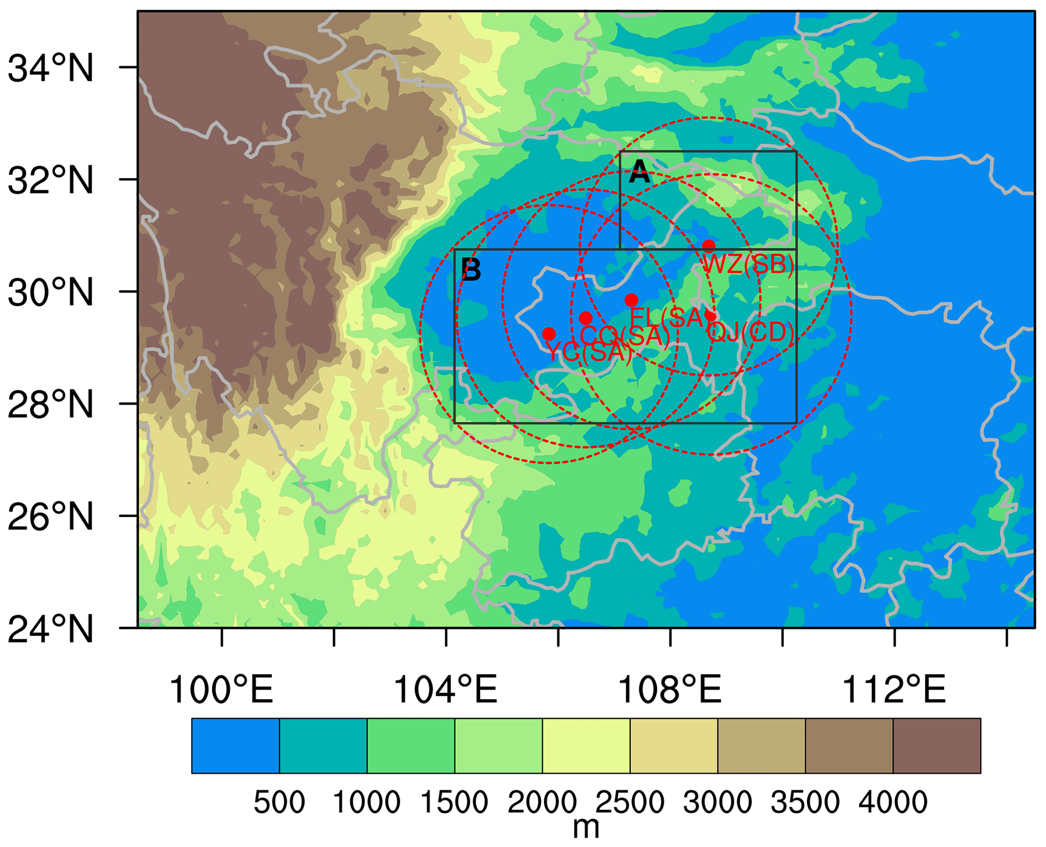
Figure 1 The inner domain and its topography (shaded; units: m) in the WRF model. The red dots and dashed red circles denote the radar stations and the coverage of the radar network, respectively. The research areas are delimited by black rectangles A and B to exclude areas that are not covered by the radar network.

The 1 km CAPPIs and CVMRs are interpolated linearly to a 5 km resolution in Fig. 2 to match the resolution of the rain rate data. Linear interpolation uses Euclidean distances as weights without the effects of terrain or the Earth's sphere. Figure 2a shows a southwest–northeast convective system captured by the CVMRs at 18:00 UTC on 28 August. Area A contains more convective cells than area B. In contrast, the 1 km CAPPIs, as shown in Fig. 2d, miss the convective cells in area A owing to terrain blockage. Although both the 1 km CAPPIs and CVMRs indicate clear geophysical boundaries between precipitation and non-precipitation areas, the CVMRs present better representations in mountainous areas. Notably, the zero gradient of hydrometeors caused by geophysical boundaries created difficulties in the application of some DA and ML algorithms.

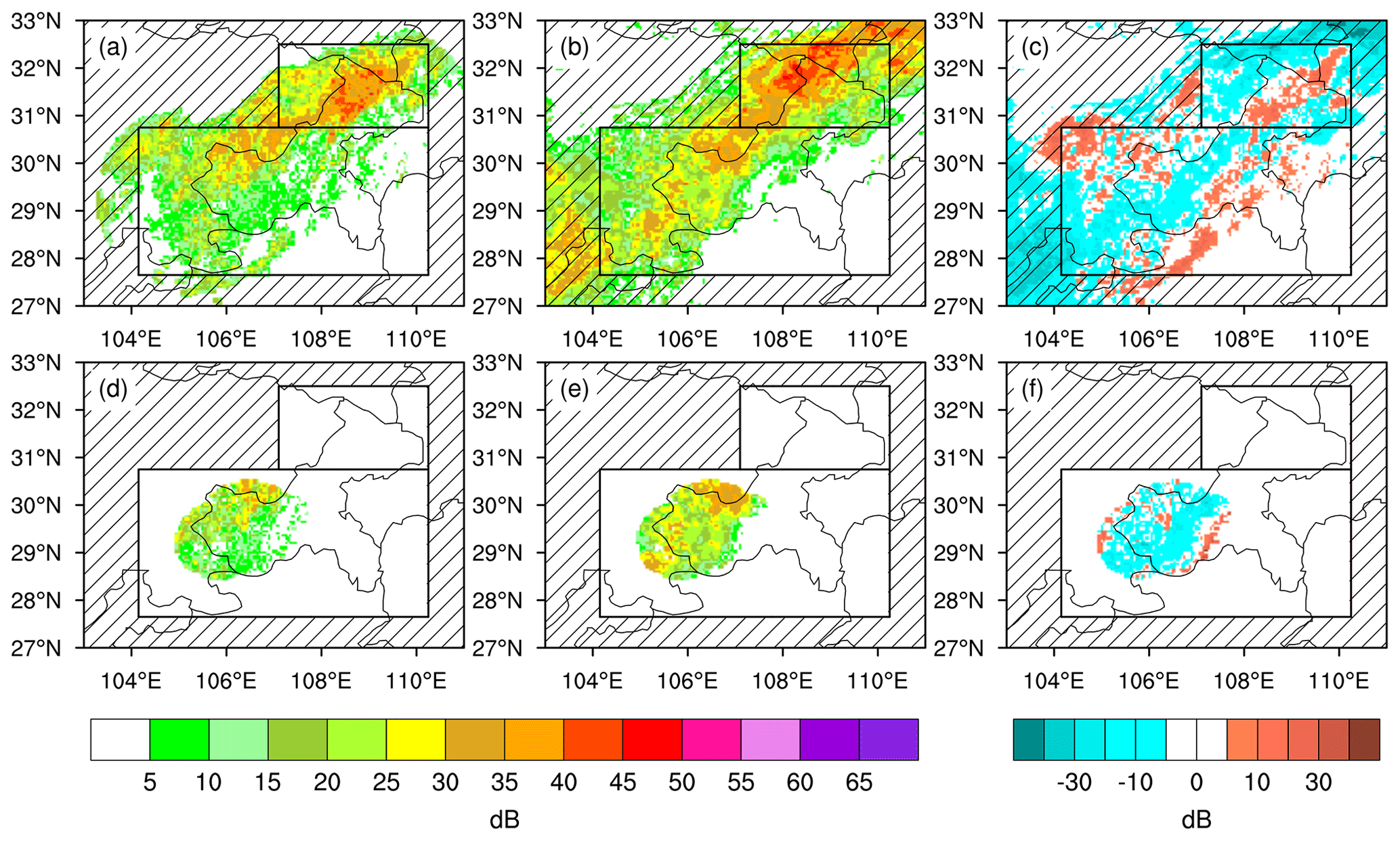
Figure 2 Distributions of CVMRs (a–c) (unit: dB) and 1 km CAPPIs (d–f) (unit: dB) observed by radars (a, d) and simulated by the model (b, e), along with their OmBs (e, f) at 18:00 UTC on 28 August 2021. The black rectangles indicate the research areas, as in Fig. 1.

2.2 Model equivalents

The 6-month model equivalents of 1 km CAPPIs and CVMRs are simulated by the Weather Research and Forecasting (WRF; Skamarock et al., 2019) model Version 4.1. The Lambert projection, whose standard latitudes are 20 and 30° N with standard longitude 106.5° E, is used. The same physics packages, including the new Kain–Fritsch scheme (Kain, 2004), the Yonsei University planetary scheme (YSU, Hong et al., 2006), the Thompson scheme (Thompson et al., 2008), and the Unified Noah Land Surface Model (Ek et al., 2003), are employed in the 6-month simulations. The WRF model has been one-way nested with a coarse resolution of 9 km and a fine resolution of 3 km. Figure 1 gives the topography in the inner domain of the WRF model, whose central location is at 29.8° N, 106.58° E and whose horizontal grids are 480×360. In the outer domain, the central location is at 30° N, 104.5° E and the horizontal grids are 600×480. Both domains have 51 vertical layers.

The initial and lateral boundary conditions of the WRF model are 0.5° × 0.5° Global Forecast System (GFS) data produced by the National Centers for Environmental Prediction. More information about GFS datasets is available at https://www.ncei.noaa.gov/products/weather-climate-models/global-forecast (last access: 1 August 2024). The GFS analyses at 00:00 and 12:00 UTC from April to September are used to drive the WRF model. The model equivalents are computed using 6 h simulations because a shorter simulation time causes spin-up issues and a longer simulation time brings large model errors. The overall growth of model errors can be described by the 6 h integration of the WRF model since various observations are assimilated by the GFS. No reflectivity assimilation has been performed here since we investigated the impacts of the symmetric error model on the climatology of representation error. The model equivalents have 12 h time intervals (i.e., 06:00 and 18:00 UTC) in this study.

The diagnostic algorithm of three-dimensional reflectivity, consisting of raindrops, snow particles, and graupel particles, can be briefly described as follows:

$$\begin{array}{}\text{(1)}& Z=\mathrm{10}{\log }_{\mathrm{10}}\left(Z_{\mathrm{er}}+Z_{\mathrm{es}}+Z_{\mathrm{eg}}\right),\end{array}$$

where Z_er, Z_es, and Z_eg are the equivalent reflectivity factors for rain, snow, and graupel droplets, respectively. This diagnostic algorithm (Stoelinga, 2005) employs 8×10⁶, 2×10⁷, and 4×10⁶ m⁻⁴ as intercept parameters for rain, snow, and graupel droplets, respectively. The densities of rain, snow, and graupel droplets are 1000, 100, and 400 kg m⁻³, respectively. The Unified Post Processor (UPP) package (https://epic.noaa.gov/unified-post-processor/, last access: 1 August 2024) interpolates diagnostic reflectivities from the coordinates of the WRF model to altitude levels and then generates the model equivalents of 1 km CAPPIs and CVMRs. Despite some empirical assumptions, this diagnostic algorithm can transform model variables, such as rain, snow, and graupel mixing ratios, to reflectivity. Liu et al. (2022) used a similar diagnostic algorithm based on double-moment Thompson microphysics as the forward operator in reflectivity assimilation.

In Fig. 2b, the model equivalents of the CVMRs capture the southwest–northeast rain belt with strong convective cells in area A, illustrating that the WRF model is capable of simulating this convective system. The CVMRs and their model equivalents still present discrepancies in the comparison of Fig. 2a and b. As shown in Fig. 2c, the OmBs can vary widely from place to place, implying that a constant standard deviation may be insufficient to describe the error structure of CVMRs. For the 1 km CAPPIs, the model equivalents (Fig. 2e) and their OmBs (Fig. 2f) present similar features to those of the CVMRs. Thus, regardless of 1 km CAPPIs or CVMRs, the model equivalents are misplaced, are ill-shaped, or have erroneous intensities compared to observations point by point. Following Geer and Bauer (2011), we refer to all these errors as “mislocation” errors. The mislocation errors of 1 km CAPPIs and CVMRs can result in a non-Gaussian error distribution that violates the Gaussian assumptions underlying some DA and ML algorithms.

2.3 Observations minus backgrounds

To represent rainy echoes, the 1 km CAPPIs and CVMRs less than 5 dB are removed in this study. Thus, the samples in Fig. 3 do not contain false simulations (i.e., simulated, but not observed). Figure 3a shows a histogram of all CVMRs against their model equivalents based on 1 165 529 samples, including missed simulations (i.e., observed, but not simulated). The high numbers along the abscissa imply the large mislocation error of CVMRs resulting from considerable missed simulations. Compared with the satellite radiance departures (Fig. 5 in Migliorini and Candy, 2019), these considerable missed simulations are associated with the worse spatial discontinuity in the CVMR OmBs. For convenience, we refer to the discontinuous scenario as “any-reflectivity”.

To examine the effects of the large mislocation error on the CVMR error structure, we removed all missed simulations and obtained 504 123 samples (Fig. 3b). We refer to this scenario as “both-reflectivity”, whose histogram is similar to the non-precipitating-cloud-affected satellite radiance observed by the AMSR-E channel 37v (Geer and Bauer, 2011). A comparison of Fig. 3a and b shows that the any-reflectivity scenario has a more complicated error structure than the both-reflectivity scenario, illustrating that the non-Gaussian error distribution in radar reflectivity assimilation is likely to be stronger than that in satellite radiance assimilation.

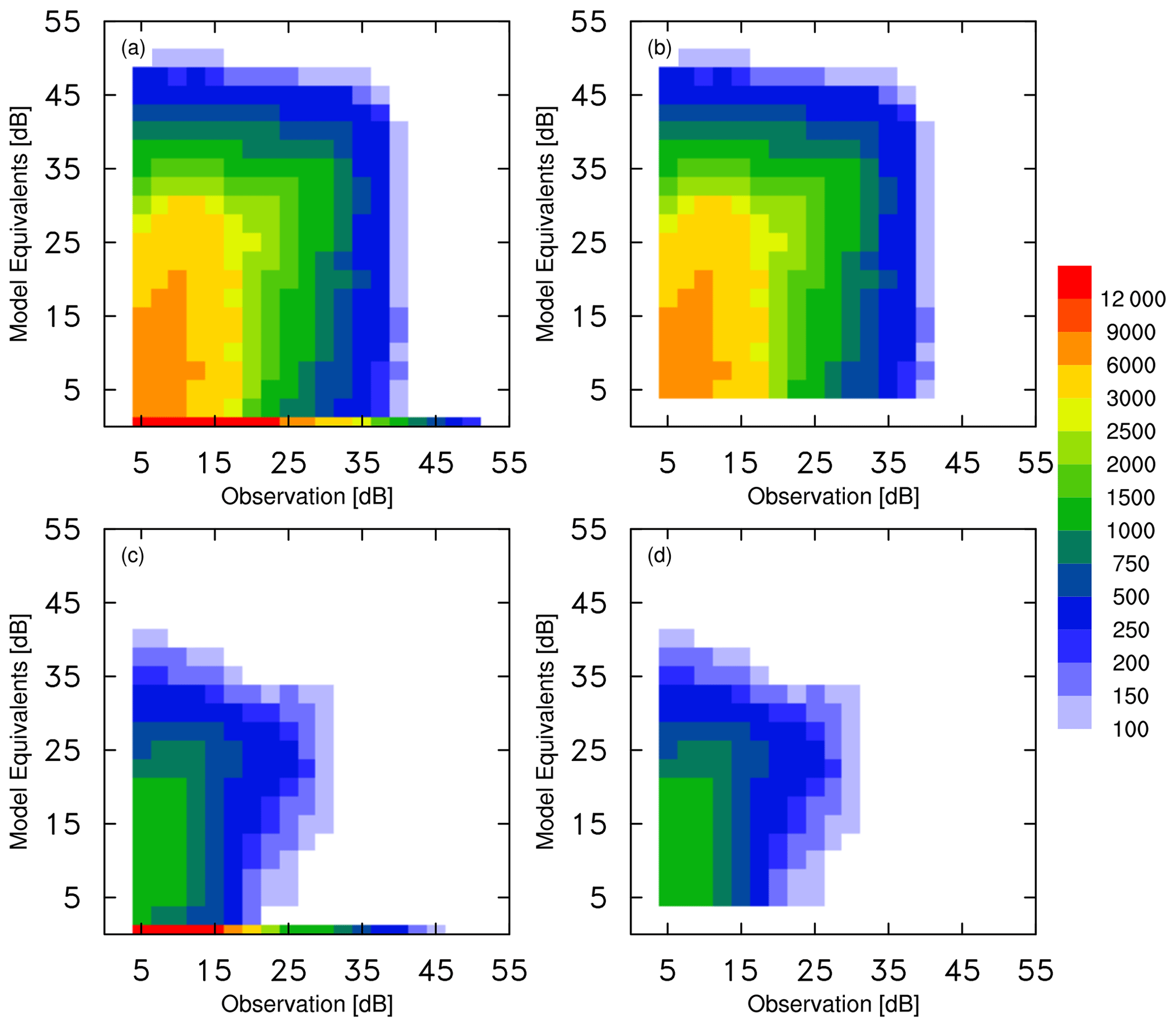
Figure 3 Histograms of the observed (a, b) CVMRs and (c, d) 1 km CAPPIs (abscissa, unit: dB) against their model equivalents (ordinate, unit: dB) in the “any-reflectivity” (first column) and “both-reflectivity” (second column) scenarios.

The sample numbers of the 1 km CAPPIs decreased to 232 681 and 71 516 for any-reflectivity and both-reflectivity, respectively. In the comparison of Fig. 3c and d, the 1 km CAPPIs also contain considerable missed simulations in terms of the high numbers along the abscissa. The error structure of the 1 km CAPPIs estimated by OmBs is similar to that of the CVMRs.

It is critical to understand the statistical features of several OmBs by examining their probability density functions (PDFs) before building a symmetric error model. Compared with the normal Gaussian distributions in Fig. 4, the PDF of CVMR OmBs (solid red line) in any-reflectivity presents a positive skewness. Instead, the PDF for both-reflectivity (solid blue line) is closer to a Gaussian distribution. The comparison illustrates that the numerous missed simulations along the abscissa in Fig. 3 have an undesirable effect on some DA and ML algorithms. In practice, the mismatches between observations and simulations provide valuable information related to convective systems. This non-Gaussian distribution cannot be ignored in radar reflectivity applications.

Similarly, the PDF of the 1 km CAPPI OmBs also approximates the Gaussian distribution after removing the missed simulations in Fig. 4. The means and standard deviations of the 1 km CAPPI and CVMR OmBs, denoted by μ and σ in Fig. 4, respectively, are similar as well. According to above comparisons, the statistical features of the 1 km CAPPI and CVMR OmBs are comparable in this study. Thus, the CVMR data in the any-reflectivity scenario are used to match the rain rate data in the following sections.

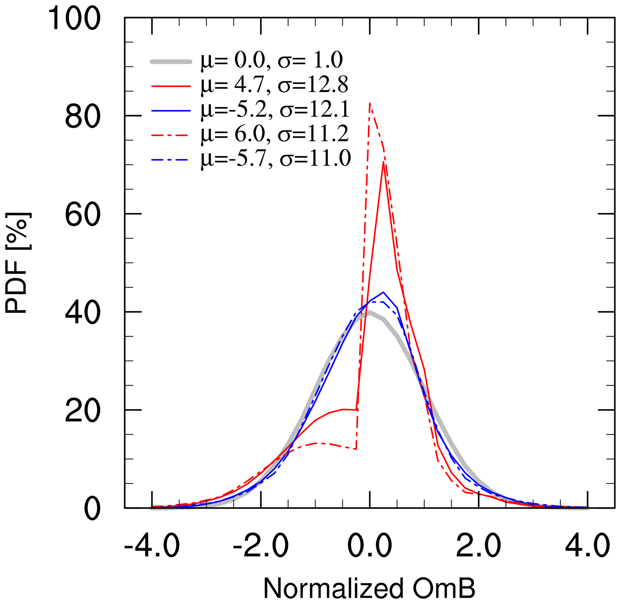
Figure 4 Probability density functions of CVMR (solid lines) and 1 km CAPPI (dashed lines) OmBs in the “any-reflectivity” (red lines) and “both-reflectivity” (blue lines) scenarios, normalized by the mean and standard deviation of all samples. The gray line represents a normal Gaussian distribution. The μ and σ symbols denote the mean and standard deviation of OmBs, respectively.

3 Predictors of the symmetric error model

3.1 Predictor derived from reflectivity

The predictors of previous symmetric error models for satellite radiance assimilation were derived from satellite radiance observations. Similarly, the rain rate can be derived from the echo signal in terms of the Z–I relationship, which is an empirical formula for estimating the rain rate I (unit: mm h⁻¹) from the equivalent reflectivity factor Z_e (unit: mm⁶ m⁻³).

$$\begin{array}{}\text{(2)}& Z_{\mathrm{e}}=a{I}^{\mathrm{b}}\end{array}$$

Here, the equivalent reflectivity factor at 3 km altitude and typical coefficients a=300 and b=1.4 are employed. Therefore, the “symmetric” rain rate, rr_sym, which is used as the symmetric predictor in this study, is the average of the derived rain rate, rr_obs, and simulated rain rate, rr_model.

$$\begin{array}{}\text{(3)}& {\mathrm{rr}}_{\mathrm{sym}}=\mathrm{0.5}\times ({\mathrm{rr}}_{\mathrm{obs}}+{\mathrm{rr}}_{\mathrm{model}})\end{array}$$

In this study, rr_model is the average of two consecutive hourly precipitation events simulated by the WRF model, not derived by the reflectivity simulation.

Figure 5 shows the distributions of the rain rate data derived from the observations and simulated by the WRF model. Despite some disagreements for CVMRs below 15 dB in area A, the derived rain belt has a southwest–northeast distribution similar to that of the actual CVMRs. Moreover, the large rainy centers in Fig. 5a are associated with the strong convective cells in Fig. 2a. The simulated rain belt in Fig. 5b also presents similarities to the model equivalents of the CVMRs in Fig. 2b. Consequently, the rain rate OmBs in Fig. 5c agree with the CVMR OmBs in Fig. 2c, illustrating that the CVMR error structure can be described by the rain rates regardless of the discrepancy between the CVMRs and rain rates.

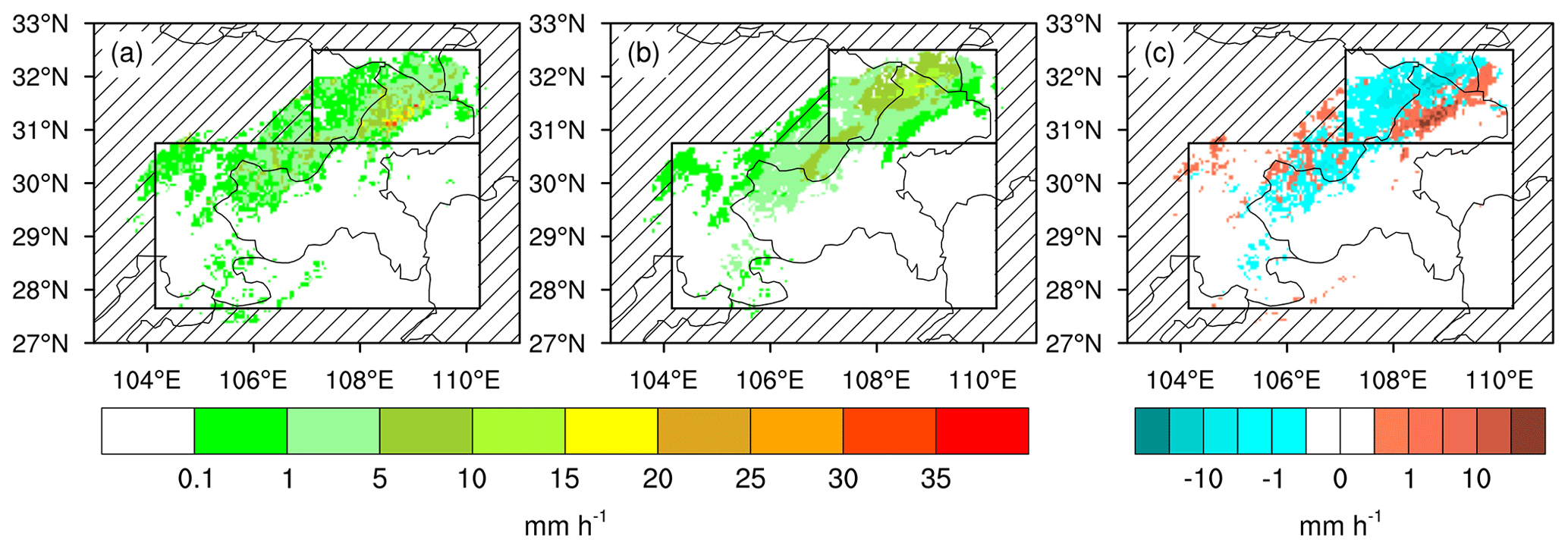
Figure 5 Distributions of rain rates (unit: mm h⁻¹) (a) derived from equivalent reflectivity factors at 3 km altitude and (b) simulated by the WRF model, along with their (c) their OmBs at 18:00 UTC on 28 August 2021. The black rectangles indicate the research areas, as in Fig. 1.

3.2 Predictors from third-party observations

Derivation from the equivalent reflectivity factor is not the only way to obtain rain rate data. Other hourly precipitation observations can be used to produce rain rate data. Thus, it is of interest to discuss how the accuracy of the rain rate affects the symmetric error model.

In this study, the derived rain rates are replaced by the CMA Multisource Precipitation Analysis System (CMPAS) data produced by the National Meteorological Information Center of the China Meteorological Administration (NMIC/CMA). Hourly CMPAS data with a 0.05° resolution, merging precipitation observations from rain gauges, radar QPEs, and satellite QPEs, capture a number of hourly precipitation details and are more accurate than other single-source precipitation observations (Pan et al., 2018; Li et al., 2022).

Comparing Figs. 5a and 6a, the CMPAS rain rates are comparable to the derived rain rates, especially for heavy precipitation in area A, because radar observations have been used to generate the CMPAS data. The CMPAS rain rates present a smoother southwest–northeast rain belt and a more evident precipitation center in the mountainous area. A few small and moderate precipitation events in area B are captured by the CMPAS rain rates, leading to a wider distribution of OmBs, as shown in Fig. 6b. Thus, more accurate precipitation data can provide more reliable samples for the construction of a symmetric error model.

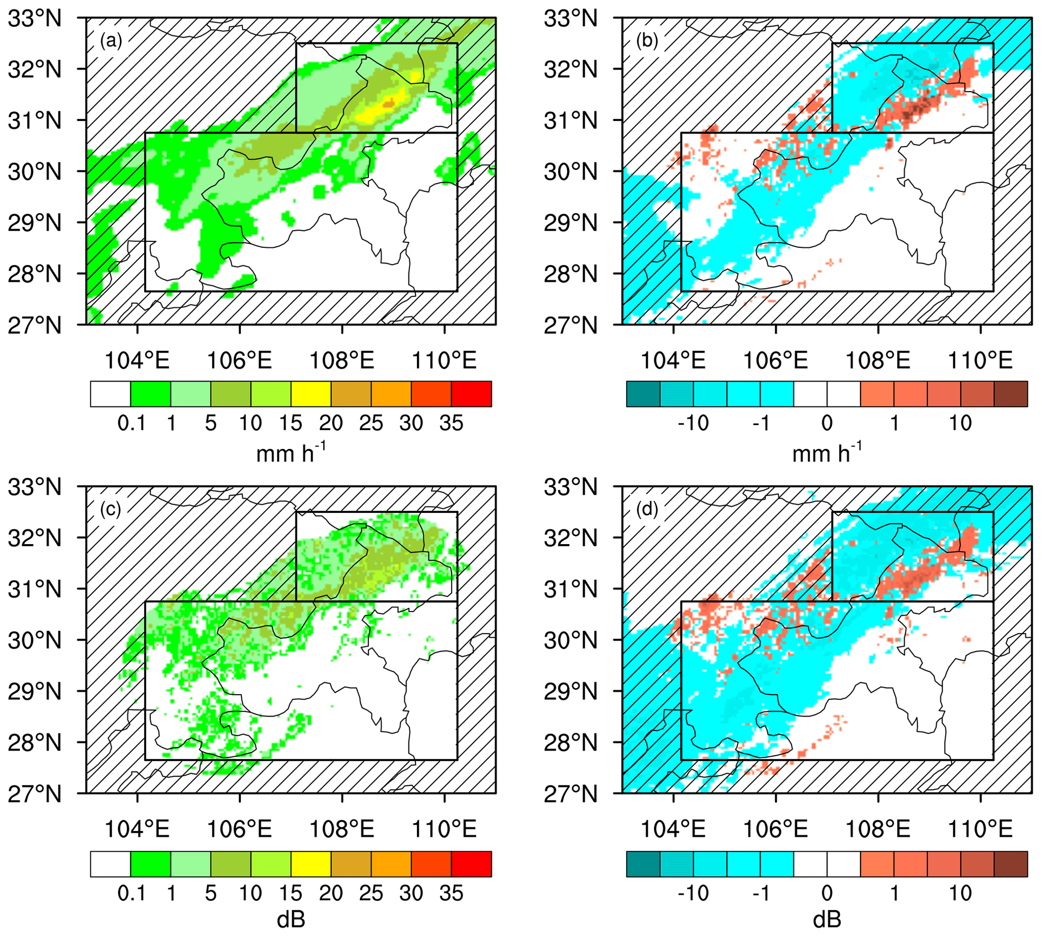
Figure 6 Distributions of (a) CMPAS rain rates (unit: mm h⁻¹) and (c) logarithmic rain rates (unit: dB) at 18:00 UTC on 28 August 2021. Panels (b) and (d) are OmBs of the CMPAS rain rates (unit: mm h⁻¹) and logarithmic rain rates (unit: dB), respectively. The black rectangles indicate the research areas, as in Fig. 1.

3.3 The linearization of predictor

The Z–I relationship exists between the rain rate I and the equivalent reflectivity factor Z_e (unit: mm⁶ m⁻³), not the reflectivity Z (unit: dB). A natural step forward is imposing a logarithmic transformation on Eq. (2) to obtain a more linear relationship between Z and I:

$$\begin{array}{}\text{(4)}& Z=\mathrm{10}{\log }_{\mathrm{10}}{Z}_{\mathrm{e}}=\mathrm{10}{\log }_{\mathrm{10}}a+\mathrm{10}b{\log }_{\mathrm{10}}I,\end{array}$$

where a and b are the coefficients of the Z–I relationship. In this study, Eq. (4) is not a formula for accurately obtaining the quantitative reflectivity. It merely transforms the relationship between the CVMRs and symmetric rain rates to a more linear relationship, which allows us to discuss the effects of the linearization of predictor on the symmetric error model. Thus, this subsection uses 10log ₁₀(I+1.0), hereafter referred to as the logarithmic rain rate (unit: dB), as a linear predictor. Adding 1.0 to the rain rate ensures that the base of the logarithm is greater than zero, which is the same as for precipitation assimilation (Lopez, 2011).

The logarithmic rain rates also present the southwest–northeast rain belt in Fig. 6c. However, the precipitation center in area A is smoothed out by the logarithm. The OmBs of the logarithmic rain rates in Fig. 6d present similar negative and positive distributions in comparison with the derived rain rates in Fig. 5c. Notably, a number of precipitation events below 0.1 mm h⁻¹ are amplified by the above logarithmic transform, resulting in more OmBs of logarithmic rain rates. The logarithmic rain rates allow us to obtain more small precipitation samples.

To examine the relationship between CVMR OmBs and symmetric rain rates, it is advisable to count the number of CVMR OmBs over discrete intervals of symmetric rain rates, chosen here to be 0.5 mm h⁻¹. Owing to the numerous missed simulations in Fig. 3a, most OmBs of the derived rain rates (Fig. 7a) and CMPAS rain rates (Fig. 7b) range from −20 to 30 dB when the symmetric rain rates are less than 0.5 mm h⁻¹. As shown in Fig. 7a, the major OmBs against derived rain rates, chosen to be larger than 500 samples, become bimodal as the symmetric rain rates increase from roughly 0.5 to 2 mm h⁻¹. The two peaks are at about 30 and −10 dB.

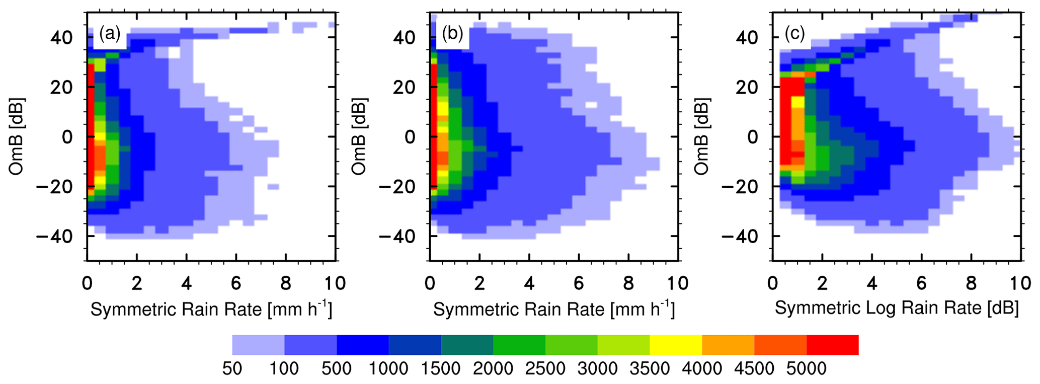
Figure 7 Histograms of CVMR OmBs (ordinate, unit: dB) against different symmetric predictors (abscissa), which are rain rates (unit: mm h⁻¹) (a) derived by equivalent reflectivity factors, (b) rain rates computed by CMPAS data, and (c) the symmetric logarithmic rain rate (unit: dB).

In contrast, the major OmBs against CMPAS rain rates in Fig. 7b exhibit a unimodal distribution peaking at about −10 dB. Although this unimodal distribution is not symmetric when the OmB equals zero, it is closer to a Gaussian distribution, confirming that more accurate CMPAS data can offer superior representation. When comparing the derived rain rates (Fig. 7a) with the logarithmic rain rates (Fig. 7c), the major OmBs exhibit a bimodal distribution but become gradual along the abscissa. As a result, the logarithmic transformation reduces the rain rate gradient without altering the structure of the CVMR OmBs.

4 Errors as a function of symmetric rain rates

4.1 The CVMR symmetric error model

Similar to satellite radiances, it is possible to investigate the CVMR error structure over discrete rain rate bins, chosen to be 0.5 mm h⁻¹ in this study. As shown in Fig. 8a, the standard deviations of the CVMR OmBs vary from about 10 to 33 dB. A constant value is insufficient to describe the CVMR error structure. The difference between the first two bins is much greater than that between the other bins. To illustrate this, we may argue that light precipitation is closer to the geophysical boundary than moderate precipitation, resulting in a greater difference between the first two bins. From the second bin, the standard deviations of the CVMR OmBs increase with symmetric derived rain rates before peaking at 8.0 mm h⁻¹. The standard deviations that alternately increase and decrease after 8.0 mm h⁻¹ could be caused by poor initial conditions of the WRF model, small sample numbers, or inaccurate diagnostic reflectivity.

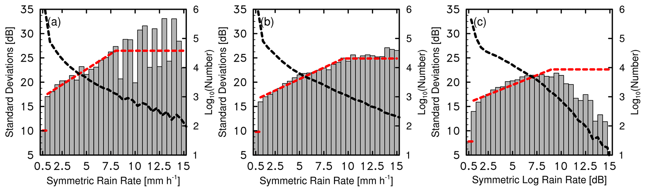
Figure 8 Standard deviations of CVMR OmBs for symmetric (a) derived rain rates (unit: mm h⁻¹), (b) CMPAS rain rates (unit: mm h⁻¹), and (c) logarithmic rain rates (unit: dB). The dashed red lines show the three-piecewise fitting functions (listed in Table 1). The dashed black lines show the logarithm of sample numbers over symmetric rain rate bins.

To simplify the complex CVMR error structure, a three-piecewise function (dashed red line) is fitted by using linear regression. The first bin must be isolated from the linear regression to pass the 95 % confidence level for the F test. A straight line rather than a linear regression is used to describe the reflectivity error for large symmetric derived rain rates. This is a cautious approach to fit a rational linear regression based on a large sample size (dashed black line), chosen to be larger than 10³ samples. Table 1 lists the key parameters of the piecewise functions.

Table 1 The key parameters of the three-piecewise fitting functions.

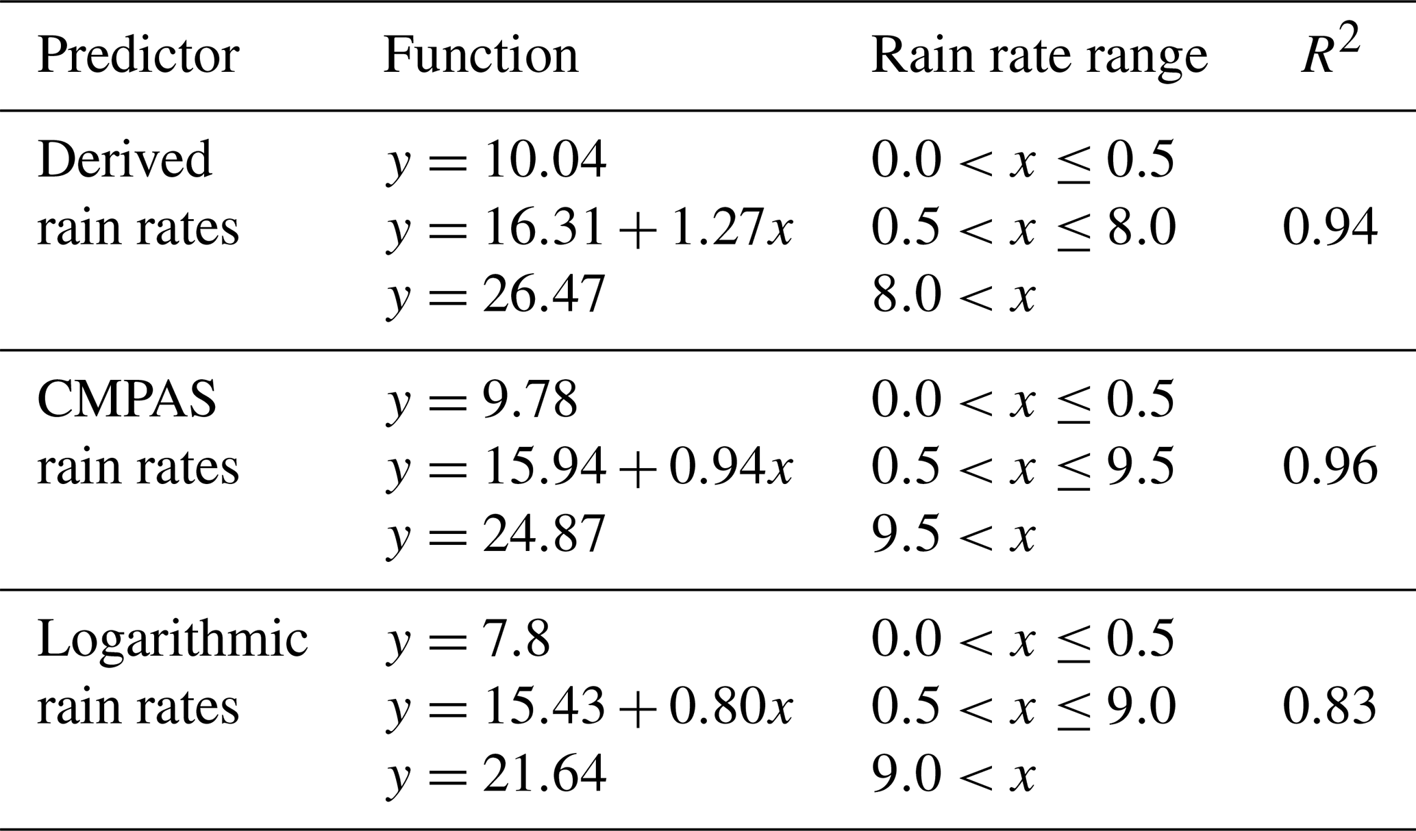
As shown in Fig. 8b, similar characteristics, such as the distinct difference between the first two bins and the increase in symmetric derived rain rates, are captured by the symmetric CMPAS rain rates as well. The standard deviations vary from about 10 to 25 dB when the symmetric CMPAS rain rate increases from 1 to 9.5 mm h⁻¹. The small variation in the standard deviations after 10 mm h⁻¹ results from the superior representation of the CMPAS data. For the symmetric logarithmic rain rates (Fig. 8c), the standard deviations of the CVMR OmBs grow gradually from roughly 14 to 21 dB as the symmetric logarithmic rain rates increase from 1 to 10, even if they still increase quickly from about 8 to 14 in the first two bins. The decreasing trend at the tail of the logarithmic rain rates (larger than 9.0) results from the rapid decrease in sample size. The straight line prevents the three-piecewise fitting function from being obtained from an irrational linear regression. According to Table 1, the logarithmic rain rates obtain the smallest slope of the fitting function among the three symmetric predictors despite having the smallest R².

4.2 Improvements in Gaussianity

To illustrate the potential benefits of symmetric error models to some DA and ML algorithms, the Gaussianity of the PDF is examined in this subsection. Although the PDF of CVMR OmBs is not Gaussian, the CVMR OmBs can be divided into a number of subgroups with Gaussian PDFs according to the binned standard deviations or piecewise functions from the above subsection. Figure 9 shows the PDFs of the CVMR OmBs normalized by various symmetric rain rates, with the raw and normal Gaussian PDFs displayed for comparison. Compared with the raw PDF (green line), the PDFs normalized by the binned standard deviations (red line) become more Gaussian. The three-piecewise function, which simplifies the CVMR error structure, also corrects the positive skewness of the raw PDF. We argue that the three-piecewise function is sufficient in this study because it shows an identical PDF to the binned standard deviations.

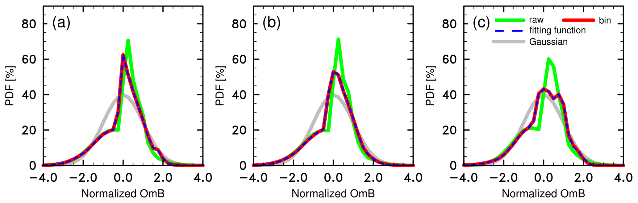
Figure 9 PDFs of CVMR OmBs normalized by symmetric (a) derived rain rates, (b) CMPAS rain rates, and (c) logarithmic rain rates. The green, red, blue, and gray lines represent the raw, binned, three-piecewise, and normal Gaussian PDFs, respectively.

To quantify the similarity between the PDF normalized by the symmetric rain rates and a normal Gaussian PDF, Table 2 lists the Jensen–Shannon divergence (JSD):

$$\begin{array}{}\text{(5)}& \begin{array}{rl}\mathrm{JSD}& (P\parallel Q)={\displaystyle \frac{\mathrm{1}}{\mathrm{2}}}\sum P\left(x\right)\log \left({\displaystyle \frac{\mathrm{2}P\left(x\right)}{P\left(x\right)+Q\left(x\right)}}\right)\\ & +{\displaystyle \frac{\mathrm{1}}{\mathrm{2}}}\sum Q\left(x\right)\log \left({\displaystyle \frac{\mathrm{2}Q\left(x\right)}{P\left(x\right)+Q\left(x\right)}}\right),\end{array}\end{array}$$

where P is the PDF normalized by symmetric rain rates or raw standard deviations and Q represents a normal Gaussian PDF. When JSD is zero, the distributions P and Q are the same. For the derived rain rates, the JSDs of the PDFs normalized by the binned standard deviations and the three-piecewise function decrease from 0.010 to 0.006.

Table 2 Jensen–Shannon divergences of probability density functions normalized by various symmetric rain rates.

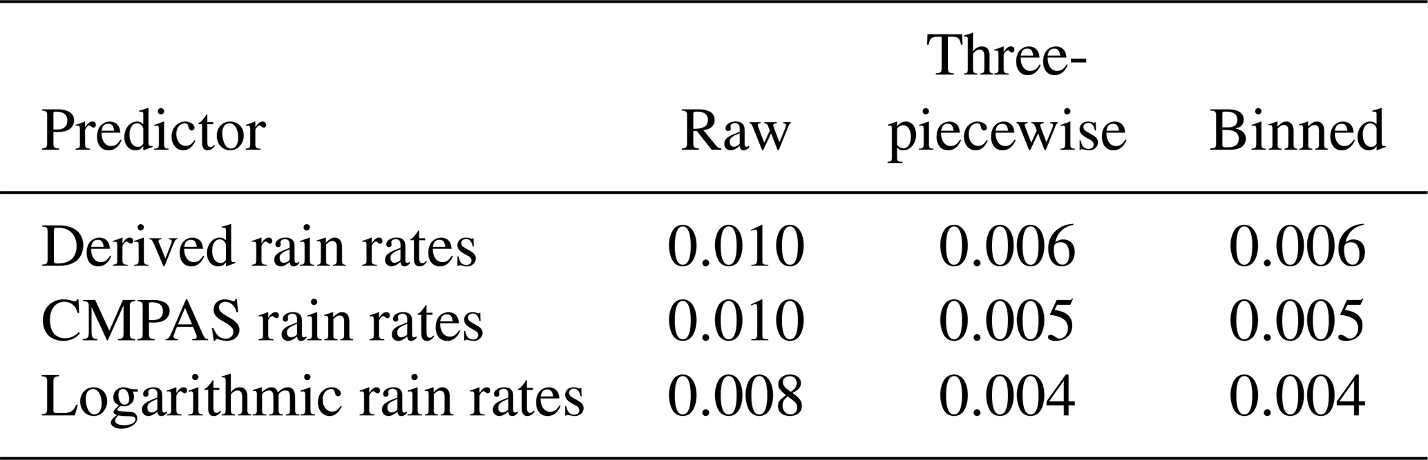
For the CMPAS rain rates in Fig. 9b, the PDFs normalized by the binned standard deviations and the three-piecewise function not only correct the positive skewness, but also reduce the overestimation in the central area. The CMPAS rain rates also have smaller JSDs than the derived rain rates, as listed in Table 2. This demonstrates that the accuracy of CMPAS rain rates can further improve the Gaussianity of the PDFs. For the logarithmic rain rates (Fig. 9c), the PDFs normalized by the binned standard deviations and three-piecewise function also approximate a normal Gaussian distribution according to comparison with the raw PDF. It is worth noting that the logarithmic rain rates obtain the smallest JSDs despite a few fluctuations in the PDFs normalized by the binned standard deviations and three-piecewise function.

5 Conclusions

In this study, the Gaussianity of two types of OmB data, i.e., the CVMRs and 1 km CAPPIs, is examined in southwestern China. Their features, such as horizontal distributions and PDFs, are similar regardless of the different definitions between the CVMRs and 1 km CAPPIs. Consequently, the 6-month CVMR OmBs, which exhibit representation superior to 1 km CAPPI OmBs in mountainous and hilly areas, are employed to discuss the handling of non-Gaussian PDFs.

In the comparison of the any-reflectivity and both-reflectivity scenarios, the Gaussianity of OmBs can be improved by removing the numerous mismatches between observations and simulations. These mismatches cannot be ignored in some DA or ML algorithms. They provide essential information related to convective systems. Moreover, the reflectivity OmBs often varies widely from place to place, demonstrating that a constant standard deviation is insufficient to describe the error structure of radar reflectivity in most studies and operations.

The symmetric error model, which has been broadly used in all-sky satellite radiance assimilation (Migliorini and Candy, 2019; Zhu et al., 2019; Shahabadi and Buehner, 2021), is built to improve the Gaussianity of CVMR OmBs. According to the symmetric derived rain rates, the standard deviations of CVMR OmBs can vary from about 10 to 33 dB. However, the instrument noise of radar is on the order of 1 dB.

Similar to satellite radiance, the standard deviations of CVMR OmBs increase with the symmetric derived rain rates, illustrating that the largest component of the CVMR OmBs comes from the poor prediction associated with clouds and rain as well as the inaccurate diagnostic algorithm of radar reflectivity in some DA and ML applications. As discussed in Geer and Bauer (2011), using the symmetric error model in reflectivity assimilation may also compensate for the inadequate background error specification of hydrometeors, which will be investigated by DA experiments in our ongoing study. In contrast to satellite radiance, the symmetric error model of CVMR data shows that the difference between the first two bins is much greater than that between the other bins, illustrating that a more complex structure, a three-piecewise function, should be formulated at the convection-allowing scale.

Compared with the raw PDF, the PDFs normalized by the binned standard deviations and the three-piecewise function become more Gaussian by reducing the positive skewness. Each subgroup of CVMR OmBs, separated by symmetric derived rain rates, approximates a Gaussian PDF despite the non-Gaussian PDF of all samples. Thus, this study demonstrates that the Gaussianity of CVMR OmBs can be improved by the symmetric error model based on the derived rain rates.

The effects of more accurate rain rate data on the symmetric error model of CVMRs are also examined in this study. Although the CMPAS rain rates build a three-piecewise function similar to that of the derived rain rates, the superior representation can further improve the Gaussianity of CVMR OmBs in terms of the JSDs in Table 2.

The logarithmic rain rates have profound effects on the symmetric error model of CVMR OmBs. Not only do the gradients of the standard deviations of CVMR OmBs decrease from the second bin, but the PDFs normalized by the binned standard deviations and the three-piecewise function also obtain the smallest JSDs compared with those of the other rain rates. It is convenient to create configuration files for the logarithmic rain rates in the operational system. Moreover, the logarithmic transform has been used to assimilate precipitation observations directly in the operational four-dimensional variation system at the European Centre for Medium-Range Weather Forecasts (Lopez, 2011). Thus, using a more linear predictor is recommended for building a symmetric error model of CVMRs.

In theory, the symmetric error models of CVMRs built in this study are more consistent with the fundamental principle of some DA and ML algorithms than a constant value. However, the symmetric error model, estimated by OmB data, highly relies on the numerical weather model, DA or ML strategy, and forward observation operator. Consequently, this study encourages readers to build an effective symmetric error model based on their own assimilation and prediction systems.

Performing several experiments to discuss the effects of symmetric error models on several DA and ML algorithms is also encouraged. The unskilled use of the symmetric error model is briefly described here:

$$\begin{array}{}\text{(6)}& \mathit{\sigma }=\left\{\begin{array}{c}{\mathit{\sigma }}_{\mathrm{l}}{\mathrm{RR}}_{\mathrm{avg}}<{\mathrm{RR}}_{\mathrm{avg}\mathrm{1}}\\ {\mathit{\sigma }}_{\mathrm{l}}+\mathit{\alpha }\mathit{\beta }\left({\mathrm{RR}}_{\mathrm{avg}}-{\mathrm{RR}}_{\mathrm{avg}\mathrm{1}}\right){\mathrm{RR}}_{\mathrm{avg}\mathrm{1}}\le {\mathrm{RR}}_{\mathrm{avg}}<{\mathrm{RR}}_{\mathrm{avg}\mathrm{1}}\\ {\mathit{\sigma }}_{\mathrm{u}}{\mathrm{RR}}_{\mathrm{avg}}\le {\mathrm{RR}}_{\mathrm{avg}\mathrm{2}},\end{array}\right.\end{array}$$

where RR_avg is the symmetric rain rate, and σ_l and σ_u are the lower and upper boundaries of the reflectivity error, respectively. β is the slope of the three-piecewise function and α is a tuning parameter, as designed by Geer and Bauer (2011). By tuning the parameter α, the representative error can either be assigned completely by the symmetric error model (α=1) or ignored (α=0). In the future, the effects of ice-phase hydrometeors on the symmetric error model of CVMRs should be considered. Polarization measurements and their combinations may provide additional information about hydrometeors.