the Creative Commons Attribution 4.0 License.
the Creative Commons Attribution 4.0 License.
 | 05 Sep 2024
How well can brightness temperature differences of spaceborne imagers help to detect cloud phase? A sensitivity analysis regarding cloud phase and related cloud properties
Bernhard Mayer
Luca Bugliaro
Ralf Meerkötter
Christiane Voigt
This study investigates the sensitivity of two brightness temperature differences (BTDs) in the infrared (IR) window of the Spinning Enhanced Visible and Infrared Imager (SEVIRI) to various cloud parameters in order to understand their information content, with a focus on cloud thermodynamic phase. To this end, this study presents radiative transfer calculations, providing an overview of the relative importance of all radiatively relevant cloud parameters, including thermodynamic phase, cloud-top temperature (CTT), optical thickness (τ), effective radius (Reff), and ice crystal habit. By disentangling the roles of cloud absorption and scattering, we are able to explain the relationships of the BTDs to the cloud parameters through spectral differences in the cloud optical properties. In addition, an effect due to the nonlinear transformation from radiances to brightness temperatures contributes to the specific characteristics of the BTDs and their dependence on τ and CTT. We find that the dependence of the BTDs on phase is more complex than sometimes assumed. Although both BTDs are directly sensitive to phase, this sensitivity is comparatively small in contrast to other cloud parameters. Instead, the primary link between phase and the BTDs lies in their sensitivity to CTT (or more generally the surface–cloud temperature contrast), which is associated with phase. One consequence is that distinguishing high ice clouds from low liquid clouds is straightforward, but distinguishing mid-level ice clouds from mid-level liquid clouds is challenging. These findings help to better understand and improve the working principles of phase retrieval algorithms.
- Article
(8364 KB) - Full-text XML
- BibTeX
- EndNote


Passive spaceborne imagers, with their wide field of view and, in the case of geostationary satellites, high temporal resolution, allow global observations of clouds. These passive instruments typically use solar and/or infrared (IR) window channels to retrieve cloud properties. The advantage of pure IR-based retrievals is that they can be applied during both daytime and nighttime (Nasiri and Kahn, 2008; Cho et al., 2009). Such IR retrievals often use brightness temperature differences (BTDs) of IR window channels to detect clouds or retrieve cloud properties like optical thickness (τ) or effective particle radius (Reff) (e.g., Inoue, 1985; Krebs et al., 2007; Heidinger et al., 2010; Garnier et al., 2012; Kox et al., 2014; Vázquez-Navarro et al., 2015; Strandgren et al., 2017).
Another cloud parameter which is often retrieved using BTDs (either alone or in combination with other measures) is the cloud thermodynamic phase (ice, liquid, mixed) (Ackerman et al., 1990; Strabala et al., 1994; Finkensieper et al., 2016; Key and Intrieri, 2000; Baum et al., 2000, 2012; Hünerbein et al., 2023; Benas et al., 2023; Mayer et al., 2024). Accurate satellite retrievals of cloud phase are important for various reasons. Firstly, the cloud phase plays an important role in cloud–radiation interactions (Komurcu et al., 2014; Choi et al., 2014; Matus and L'Ecuyer, 2017; Ruiz-Donoso et al., 2020; Intergovernmental Panel on Climate Change, 2021; Cesana et al., 2022). Several studies highlight its impact on climate sensitivity within general circulation models (Gregory and Morris, 1996; Doutriaux-Boucher and Quaas, 2004; Cesana et al., 2012; Tan et al., 2016; Bock et al., 2020). Accurate observations of the cloud phase are thus essential to improve cloud representation in climate models (Cesana et al., 2015; Atkinson et al., 2013; Matus and L'Ecuyer, 2017; Bock et al., 2020). Additionally, determining cloud phase is often a prerequisite in the remote sensing retrieval of cloud properties, including τ, Reff, and water path (Marchant et al., 2016).
However, determining cloud parameters such as the thermodynamic phase from BTDs is a challenging task. Radiative transfer through clouds and the atmosphere is complex, with many parameters that can in principle influence satellite observations. Although radiative transfer models are capable of correctly accounting for all of these quantities, the relative importance of these parameters is often not fully understood.
Ackerman et al. (1990) were the first to observe a correlation between BTDs in High-Resolution Interferometer Sounder (HIS) data and the different cloud phases as determined by concurrent lidar data. They proposed a trispectral technique to distinguish between ice, water, and clear sky using the BTDs between channels at about 8 and 11 µm (BTD(8.0–11.0)) and between channels at about 11 and 12 µm (BTD(11.0–12.0)). Strabala et al. (1994) expanded on their findings using MODIS airborne simulator data. They considered clouds of varying τ and found that distinguishing between ice and water clouds using these BTDs is difficult for optically thin clouds. Parol et al. (1991) and Dubuisson et al. (2008) studied the sensitivity of BTDs to effective radius Reff and particle shape for cirrus clouds. Parol et al. (1991) found that the BTD(11.0–12.0) for the Advanced Very High Resolution Radiometer (AVHRR) aboard the NOAA satellites is sensitive to whether cloud particles are spherical or non-spherical. Dubuisson et al. (2008) showed that the impact of different non-spherical ice crystal shapes on BTD(10.6–12.0) and BTD(8.7–10.6) from the Infrared Imaging Radiometer (IIR) aboard CALIPSO is small compared to their sensitivity to Reff. The effect of Reff on the BTDs was also considered by Baum et al. (2000), who further extended the trispectral method for MODIS phase retrievals by incorporating information about the horizontal variability of the BTDs. Similar to the study of Strabala et al. (1994), the radiative transfer simulations of Baum et al. (2000) primarily focused on low-level water clouds and high cirrus clouds and did not consider mid-level clouds. To bridge this gap, Nasiri and Kahn (2008) conducted a sensitivity study that also considered mid-level clouds for the MODIS BTD(8.5–11.0). They showed that BTD(8.5–11.0) is sensitive to cloud-top height (CTH) and that this leads to limitations in the phase discrimination in the cloud temperature regime where both liquid and ice can exist.
These studies show that many different parameters influence the BTDs: cloud parameters considered in previous studies include thermodynamic phase, τ, Reff, ice crystal habit, and CTH. As outlined above, most of the studies so far, however, have each focused on only a small number of these cloud parameters; an overview of the relative importance of all these cloud parameters is still missing. The influence of CTH or cloud-top temperature (CTT) on BTDs has especially not been studied in detail, with exception of Nasiri and Kahn (2008). Besides cloud parameters the amount of water vapor in the atmosphere (mainly above the clouds) also affects BTDs even in the (relatively) transparent spectral window region of 8–12 µm. This has been pointed out by several authors (Strabala et al., 1994; Nasiri and Kahn, 2008; Dubuisson et al., 2008), but the relative importance of atmospheric absorption compared to cloud parameters for BTDs has not been studied systematically.
In addition, the origin of the dependence of BTDs on cloud thermodynamic phase, as observed in satellite measurements and radiative transfer results, is not fully understood. Although phase retrievals are usually based on accurate radiative transfer calculations that take into account all radiative effects, it is argued that variations in the refractive indices of ice and water across the infrared window cause the BTDs to be sensitive to cloud phase (Finkensieper et al., 2016; Key and Intrieri, 2000; Baum et al., 2000, 2012). However, besides these effects of the cloud phase, the phase also correlates with other cloud parameters like CTT and Reff, which in turn have large effects on the BTDs as mentioned above. It is not fully understood which cloud parameters dominate the response of the BTDs in given cloud scenarios. Additionally, traditional explanations of the phase dependence of BTDs have often neglected scattering effects, which as we will show can be substantial. Thus, it is not well understood which physical processes are responsible for the observed phase dependence of the BTDs. A full understanding of the satellite channel dependencies, however, is critical to designing optimal cloud (phase) retrievals and to understanding their limitations.
To compute BTDs, satellite radiances are first transformed into brightness temperatures (BTs). This transformation by means of Planck's radiation law is a nonlinear function. As nonlinear functions can lead to unexpected behavior, we expect that there are some effects of the nonlinear relationship between satellite radiances and BTs on BTDs. To our knowledge, the effect of this nonlinear relationship has not been analyzed before.
We use radiative transfer (RT) calculations to study two BTDs of the Spinning Enhanced Visible and Infrared Imager (SEVIRI) aboard Meteosat Second Generation (Schmetz et al., 2002): the BTDs between the IR window channels centered at 8.7 and 10.8 µm (BTD(8.7–10.8)) and between those centered at 10.8 and 12.0 µm (BTD(10.8–12.0)). These are the BTDs that are mainly used to identify cloud-top phase and determine (ice) cloud properties. Figure 1 shows an example scene from SEVIRI as an RGB composite and the two BTDs for the same scene. In this study we first investigate the effect of the nonlinear relationship between radiances and BTs on the BTDs. We then use the RT calculations to analyze dependencies and sensitivities of the BTDs with respect to all radiatively important cloud parameters, namely phase, CTT, Reff, ice crystal habit, and optical thickness (τ) at 550 nm, disentangling effects of cloud particle scattering and absorption. We also consider the effect of water vapor in the atmosphere on BTDs by comparing the computed BTDs with scenarios without molecular absorption. The findings of these RT calculations are then used to analyze the information content of the BTDs with respect to cloud phase. Overall in this study we focus on the effect of cloud parameters; the effects of other parameters like viewing angle, surface emissivity, and atmospheric temperature profiles are not studied.
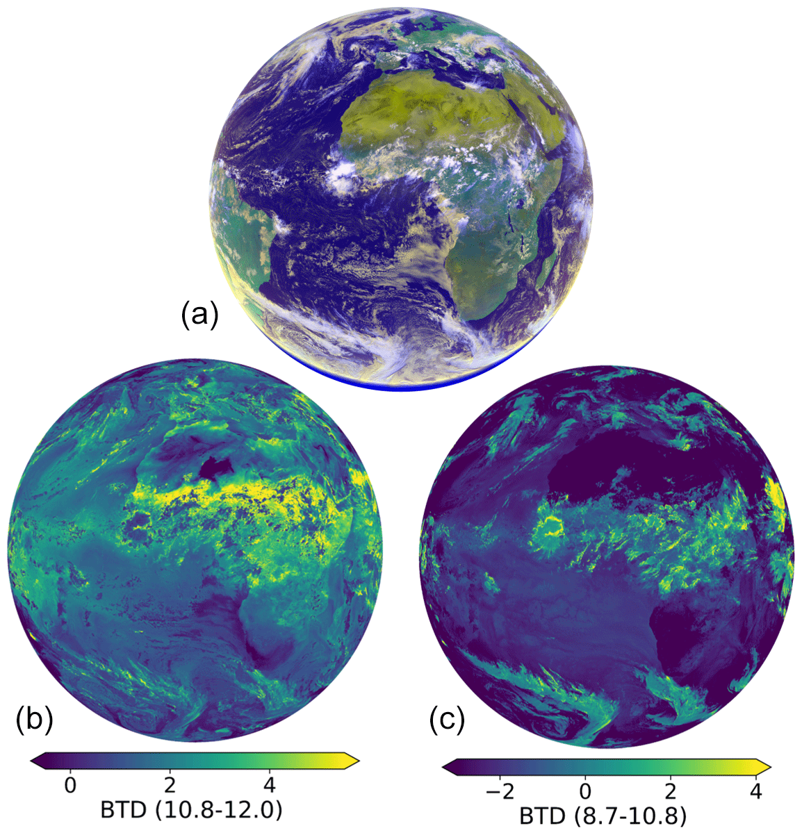
Figure 1Example scene from SEVIRI on 11 June 2023 at 12:00 UTC. (a) RGB composite with yellow cloud colors indicating higher CTTs and white–blue indicating lower CTTs. (b, c) The two BTDs for the same example scene.
The aim of this study is twofold: first, it provides an analysis of the effects of all cloud parameters on the two BTDs, disentangling the interactions among the different parameters. Second, this study improves the physical understanding of the role of the different radiative processes leading to different BTD values. This helps to understand the information content of the BTDs with respect to the thermodynamic phase in order to better understand and improve the working principles of phase retrieval algorithms that use BTDs and to understand their uncertainties and limitations. We focus on the phase, but our results are also useful to better understand the dependencies of BTDs for other remote sensing applications where they are typically used, such as the retrieval of τ and Reff. Since BTDs also depend on atmospheric and surface parameters whose effects are not studied here, this study does not aim at explaining every phenomenon encountered with BTDs. However, understanding the effects of the cloud parameters helps to disentangle different physical cloud-related processes in all atmospheric or surface conditions.
Finally, we note that besides BTDs, there are other popular methods for retrieving cloud phase and other cloud properties, such as β ratios (Parol et al., 1991; Pavolonis, 2010; Heidinger et al., 2015). While this study is specifically aimed at BTDs, understanding the effects of different cloud properties on the radiative transfer through clouds is also useful to better understand the physics underlying β-ratio retrievals.
To visualize relationships and dependencies between radiation at the top of the atmosphere (TOA) and cloud properties, the representation in the form of a causal diagram is very useful. Figure 2 shows cloud parameters that are related to the cloud phase, connected by arrows indicating causal relationships. Other factors influencing the radiation at TOA (in particular passive satellite observations), like satellite viewing angles, surface temperature, and atmospheric properties, are summarized under “other” in the diagram.
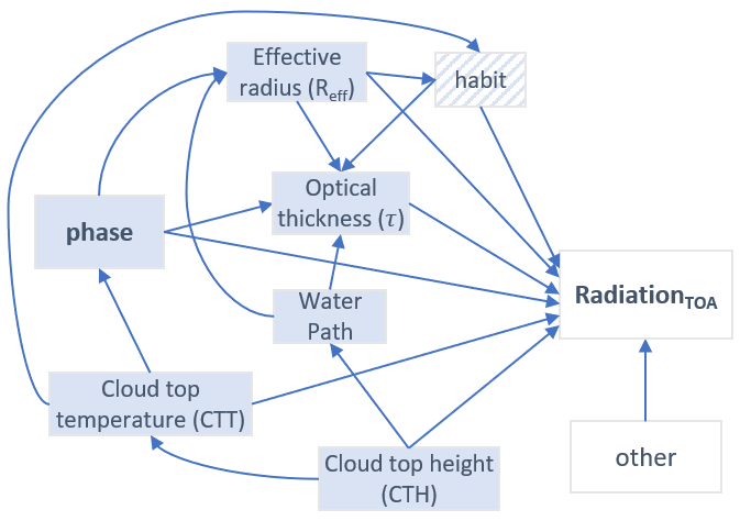
Figure 2Causal diagram of cloud parameters that are connected to the cloud phase. Arrows indicate causal links.
In this paper we use the terms “direct” and “indirect” influence of the cloud phase on the TOA radiation. Direct influence means the effect of changing the cloud phase while all other cloud parameters (Reff, CTT, τ, ...) remain the same (represented by the arrow from phase to TOA radiation in Fig. 2). The indirect influence of the cloud phase is represented by all other paths from phase to TOA radiation in Fig. 2. For example, the phase affects τ and Reff, which in turn affect TOA radiation. Information on these two parameters can give an indication about the cloud phase – e.g., clouds with small Reff are typically liquid clouds; clouds with very low τ are typically ice clouds. Ice crystal habit can influence the TOA radiation as well but is of course only relevant for ice clouds. CTT and CTH are closely related variables that influence radiation through temperature-dependent cloud emissions and by affecting the atmospheric column above the cloud that can absorb radiation, respectively. CTT is critical for phase determination since for temperatures above 0 °C only liquid is physically possible and below −40 °C only ice is physically possible. Between these thresholds, the probability for ice (liquid) clouds increases (decreases) as CTTs get colder (Mayer et al., 2023).
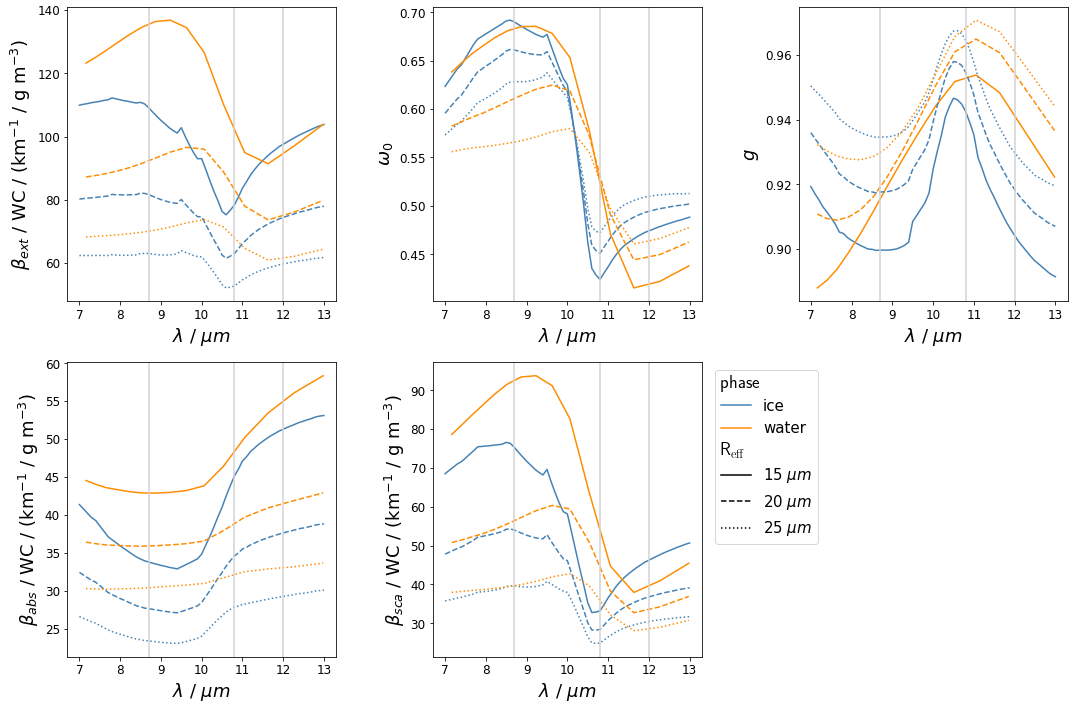
Figure 3Single-scattering properties: extinction coefficient βext, single-scattering albedo ω0, and asymmetry parameter g, as well as absorption coefficient βabs and scattering coefficient βsca (computed from βext and ω0) as functions of wavelength for varying cloud phase and effective radius Reff. βext, βabs, and βsca are scaled by the cloud water content, WC. Parameterizations for ice are according to Baum et al. (2011) and for liquid droplets according to Mie theory. For ice clouds, the “general habit mix” was used as the ice crystal habit. Vertical gray lines indicate the center wavelengths of the three IR window channels.
In order to calculate the radiative transfer through a cloud with given cloud (microphysical) parameters, it is necessary to know how much radiation is absorbed, scattered, and emitted, i.e., the optical properties of the cloud. The translation from cloud (microphysical) parameters to optical parameters is given by the so-called single-scattering properties. The single-scattering properties are the volume extinction coefficient βext, the single-scattering albedo ω0, and the scattering phase function p. As an alternative to βext and ω0 one can equivalently describe radiative transfer by the absorption coefficient βabs and scattering coefficient βsca, which can be easier to interpret. Definitions and physical interpretations of the single-scattering properties can be found in Appendix A. The interplay of the single-scattering properties, in combination with the cloud water path, determines how much radiation is transmitted through a cloud and, in combination with the cloud temperature, how much radiation is emitted from it. The single-scattering properties depend on the wavelength of the radiation and on the cloud parameters Reff, habit, and phase. They are shown in Fig. 3 for varying Reff and cloud phase. The variations of the single-scattering properties due to habit are mostly small in comparison and therefore not shown. Instead of p we show the asymmetry parameter g as a simpler measure to characterize the scattering process (see Appendix A). The spectral variations of βabs, βsca, and g translate into different BTD values for different cloud parameters. This will be investigated in detail in the next sections using radiative transfer calculations.
Simulations for the three IR window channels of SEVIRI centered at 8.7, 10.8, and 12.0 µm were performed for a variety of water and ice clouds using the sophisticated radiative transfer package libRadtran (Mayer and Kylling, 2005; Emde et al., 2016; Gasteiger et al., 2014). The libRadtran package represents water and ice clouds in detail and realistically. It has been validated against observations and in several model intercomparison campaigns and has been extensively used to develop or validate remote sensing retrievals (e.g., Mayer et al., 1997; Meerkötter and Bugliaro, 2009; Bugliaro et al., 2011, 2022; Stap et al., 2016; Piontek et al., 2021b). The optical properties of water droplets are calculated using Mie theory. For ice crystals, we use the Baum et al. (2011) parameterization of optical properties for three different habits (general habit mixture, columns, rough aggregates). Simulations of TOA radiances for the SEVIRI IR window channels are made using the one-dimensional radiative transfer solver DISORT (Discrete Ordinate Radiative Transfer) 2.0 by Stamnes et al. (2000) and Buras et al. (2011) with parameterized SEVIRI channel response functions as described by Gasteiger et al. (2014). The complete permutation of τ, Reff, CTT and CTH, crystal habits, and phase was simulated and is listed in Table 1. The CTT is set to the atmospheric temperature at the altitude of the CTH and represents the temperature at cloud top. For simplicity we keep the cloud geometric thickness constant at 1 km; the impact of variable geometric thickness is discussed in Sect. 6.3. We only consider single-phase (ice or water) and single-layered clouds. True mixed-phase clouds and multilayered clouds are not considered.
Baum et al. (2011)Table 1Setup and cloud properties for libRadtran radiative transfer calculations (SATZ: satellite zenith angle, SKT: skin temperature).
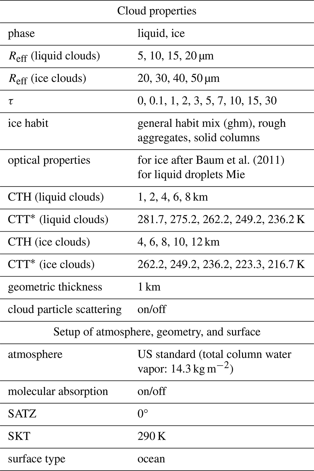
∗ Corresponds to CTH.
The simulation setup in terms of atmosphere, satellite and solar geometry, and surface type is summarized as well in Table 1. In this study, we focus on the influence of cloud parameters. Therefore, we choose a relatively simple setup for the atmospheric parameters, surface parameters, and satellite geometry, which is kept constant for all simulations. We use the US standard atmosphere (Anderson et al., 1986) and a surface temperature of 290 K. We place the simulations over the ocean where the surface emissivity is nearly constant for the three IR window channels and set it to 1. The satellite zenith angle (SATZ) is kept constant at 0° (nadir view).
To disentangle cloud effects from effects of the atmosphere, we also compute simulations with molecular absorption switched off. The libRadtran package further has the possibility of simulating the IR window channels for cloud layers for which scattering is switched off, meaning that the scattering coefficient in the simulation is set to zero while the absorption coefficient remains constant. This allows disentangling the effects of scattering and absorption in a cloud.
Before analyzing the results of the RT calculations, we examine the effects of the nonlinear relationship between radiances and BTs on the BTDs. We call these effects the BTD nonlinearity shift. The BTD nonlinearity shift is purely due to the nonlinearity in the computation of BTDs and not due to wavelength-dependent optical properties of the cloud, which we will focus on in the next sections of this study. BTDs are calculated from measured radiances using Planck's radiation law, which describes the spectral radiance Bλ of a black body emitting radiation at temperature T:
where h is the Planck constant, c is the speed of light in a vacuum, and kB is the Boltzmann constant. The inverse Planck function accordingly maps spectral radiance Rλ to the corresponding temperature,
and is used to compute BTs from measured radiances in remote sensing.
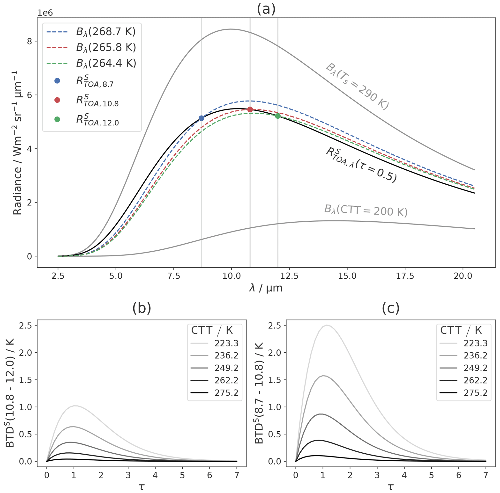
Figure 4(a) Radiance at the top of the atmosphere () computed with the Schwarzschild equation (black line). Vertical gray lines indicate the center wavelengths of the three IR window channels with blue, red, and green dots at , , and , respectively. The dashed blue, red, and green lines correspond to the Planck curves of these three TOA radiances, i.e., for each wavelength, where Bλ is the Planck function and Tλ the inverse Planck function. The solid gray curves show the Planck curves of the surface temperature Ts and the CTT as a reference. (b) Brightness temperature differences computed with the Schwarzschild equation, BTDS, as functions of τ for different CTTs and a fixed Ts=290 K.
The simplest version of the BTD nonlinearity shift can be explained using the Schwarzschild equation for radiative transfer. The Schwarzschild equation is a simple version of radiative transfer assuming no cloud scattering and no atmosphere. Its solution for one cloud layer is
where is the radiance at TOA at a given wavelength λ with the superscript S for Schwarzschild, and τλ is the optical thickness of the cloud for this wavelength. The first term in the equation is the transmitted radiance coming from the surface with the surface temperature Ts; the second term is the radiation emitted by the cloud, assuming that the cloud layer has an approximately constant temperature T≈CTT. To demonstrate the BTD nonlinearity shift we set τλ as equal for all wavelengths, τλ=τ. Figure 4a shows the Planck function of the surface temperature, Bλ(Ts), and the cloud temperature, Bλ(CTT), in gray for exemplary values of Ts=290 K and CTT=200 K. According to the Schwarzschild equation (Eq. 3), lies between these two curves, approaching Bλ(Ts) for τ→0 and Bλ(CTT) for τ→∞. Figure 4a illustrates for τ=0.5 (black line). From we can now compute the TOA BTs at the three IR wavelengths of interest as BT, where the superscript S again stands for Schwarzschild. The corresponding Planck curves, i.e., for , are shown in Fig. 4a as dashed colored lines. Recall that in this example calculation we have set a constant τ=0.5, i.e., the same optical properties (transmittance and emissivity) for all wavelengths (see Eq. 3). Naively, one might expect BTD=0 (i.e., equal BTs) in this scenario. However, it is evident from the figure that the three BTs are different, with . Since these differences between the three BTs are not due to optical cloud properties, they must be caused by the nonlinear transformation from radiances to BTs. Hence, the BTD nonlinearity shift induces a BTD in situations where, naively, no BTD would be expected.
To get an overview of the BTD nonlinearity shift, we compute BTDS for both wavelength combinations (BTD(8.7–10.8) and BTD(10.8–12.0)) from the results of the Schwarzschild equation (Eq. 3) for varying τ and CTT as
Figure 4b shows the computed BTDS as a function of τ for different CTTs and a fixed Ts=290 K. These BTDS resemble an arc shape (similar to the well-known BTD arc from Inoue, 1985) and show higher values for lower CTTs, even though the amplitudes of their curves are smaller than for the full RT model, as we will see later. Thus, even if τλ is the same for all three wavelengths, τλ=τ, the nonlinearity of the inverse Planck function induces positive BTDS values and a dependence on the CTT. More generally, this dependence is mainly a sensitivity to the thermal contrast ; however, for a fixed Ts, as shown in the examples here, it reduces to a dependence on CTT. Notice that for these examples the BTD induced this way reaches up to 2.5 K and thus cannot be neglected.
In the next section we will discuss the effects of cloud properties on the BTDs due to the wavelength-dependent optical properties in the full RT model (described in Sect. 3). The BTD nonlinearity shift adds to these effects and is therefore co-responsible for the (positive) BTD values and the CTT dependence of the BTDs, which we will discuss in more detail in Sect. 5.6. In Appendix B we further analyze the BTD nonlinearity shift for the Schwarzschild model as well as the full RT model and disentangle this nonlinearity effect from the physical effects of wavelength-dependent optical properties on the BTDs in RT calculations.
This section can be summarized as follows.
-
There is an effect (BTD nonlinearity shift) coming from the nonlinearity of the inverse Planck function that induces positive BTD(8.7–10.8) and BTD(10.8–12.0) values and a dependence on the CTT (or more generally the surface–cloud temperature contrast ΔT) in a simple RT model (Schwarzschild equation) even if cloud optical properties (transmittance and emissivity) are the same for all wavelengths.
In this section we analyze the results of the RT calculations described in Sect. 3. We start with the effects of scattering on the BTs of the three window channels separately. We then combine the BTs to BTDs and analyze them as functions of τ, phase, Reff, ice crystal habit, and CTT, focusing on the physical relationships between these cloud properties and the BTDs. In order to disentangle the effects of the different cloud parameters, we always vary only one or two parameters and keep the remaining cloud parameters at fixed “default” values, namely CTH=6 km (corresponding to CTT=249.2 K) and Reff=20 µm for both cloud phases and the general habit mix as the ice crystal habit.
The following conventions are used throughout this section: blue indicates the ice phase, and orange–red colors indicate the liquid phase. Solid lines represent a “normal” atmosphere with molecular absorption, and dashed lines mean that molecular absorption is switched off.
5.1 Effects of scattering on brightness temperatures
Scattering in the infrared window only needs to be considered for cloud particles; Rayleigh scattering by atmospheric molecules is negligible in the infrared window. The effects of cloud particle scattering on the BTs are shown in Fig. 5. It shows the difference between the BTs for a cloud with scattering and a cloud with scattering switched off for the three window channels, i.e., for each channel with center wavelength λ. This is shown as a function of τ (at 550 nm) for an ice and a water cloud with all other cloud parameters held constant. Switching off scattering in a cloud changes the optical thickness of that cloud, since only absorption now contributes to the extinction of radiation. However, to be able to compare scenarios with and without scattering for fixed cloud microphysics (same water content and Reff), the τ parameter used for this figure is still the “original” optical thickness (with absorption and scattering).
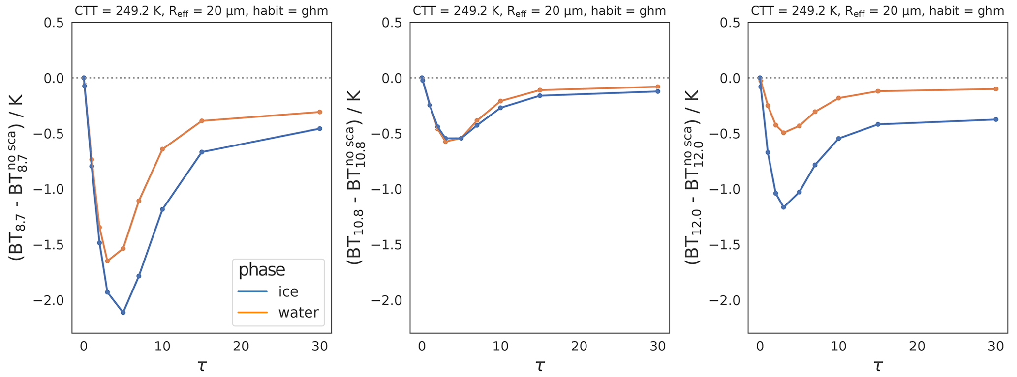
Figure 5Scattering effects on brightness temperatures (BT): difference between the BTs for a cloud with scattering and a cloud with scattering switched off for all three IR window channels, i.e., for each channel with center wavelength , for liquid and ice clouds as functions of optical thickness τ.
All curves in Fig. 5 are negative everywhere, meaning that scattering is a radiation sink for all three wavelengths: part of the radiation coming from below the cloud is scattered back downwards. However, the amount of radiation lost to scattering is different for the different wavelengths. Scattering has a larger effect on the radiation at 8.7 µm than at 10.8 or 12.0 µm, as expected from βsca which is higher at 8.7 µm than at the other two wavelengths (see Fig. 3). For 8.7 and 12.0 µm, scattering by ice clouds is more significant than by water clouds; for 10.8 µm, scattering leads to a similar radiation loss for both water and ice clouds. Interestingly, scattering effects are visible even when the cloud is opaque (black, τ=30). An explanation is that the observed radiance at TOA does not just come from the top of the cloud. Rather, it comes from the upper layers within the cloud (with decreasing intensity as one moves deeper into the cloud). Radiation emitted anywhere below the cloud top is still subject to scattering on its way to the cloud top.
Using different CTT or Reff values in the calculations (for both the liquid and the ice cloud) mainly changes the magnitude of the negative peaks but does not change the qualitative results shown in Fig. 5. Similarly, changing the ice crystal habit does not change the qualitative results and has only a small effect on the values shown.
5.2 Effects of optical thickness on BTDs
We begin the study of BTDs by analyzing the physical factors that drive the BTD behavior in relation to τ. Figure 6 shows BTD(8.7–10.8) and BTD(10.8–12.0) as functions of τ for both an ice and a liquid cloud and with molecular absorption switched on and off.
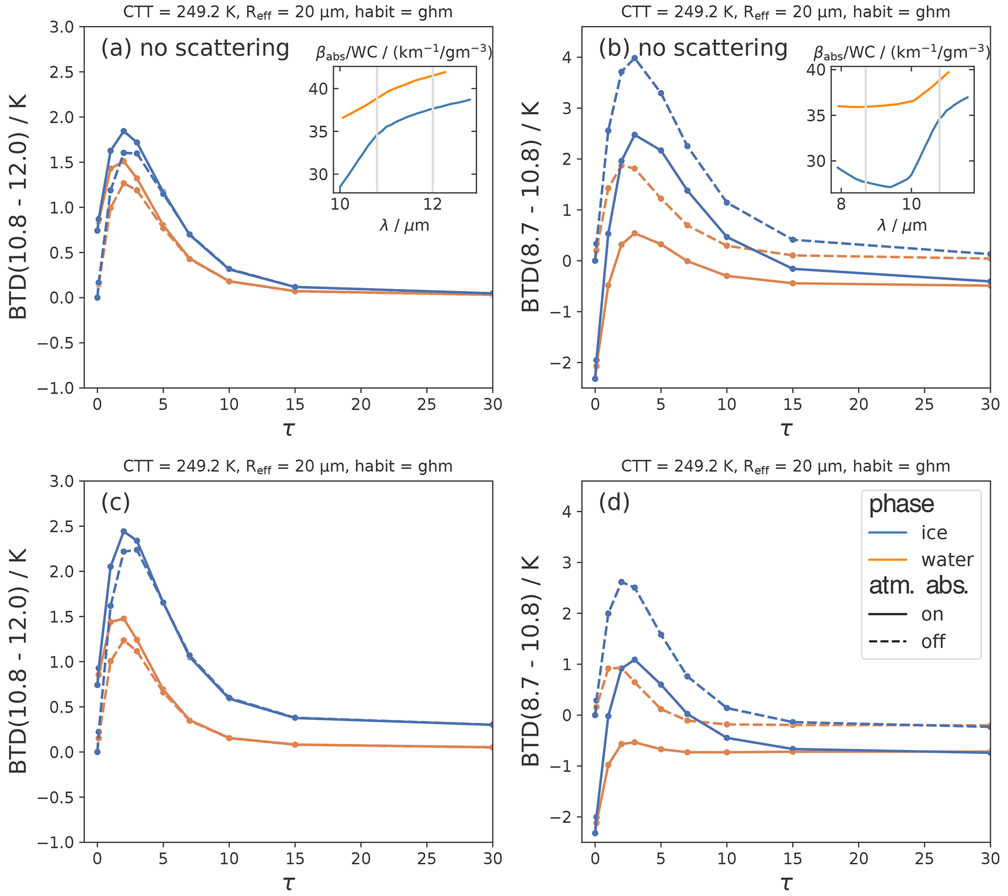
Figure 6Brightness temperature differences BTD(10.8–12.0) and BTD(8.7–10.8) as functions of τ for cloud particle scattering (a, b) switched off and (c, d) switched on for liquid and ice clouds. Solid lines indicate a “normal” absorbing atmosphere, and dashed lines indicate that molecular absorption is switched off.
As τ approaches zero in all panels of Fig. 6, i.e., no cloud is simulated, the BTD curves with atmospheric absorption switched on (solid lines) do not go to zero. They remain above zero for BTD(10.8–12.0) and below zero for BTD(8.7–10.8). This is the effect of atmospheric absorption, since radiation at 8.7 and 12.0 µm is more strongly absorbed by water vapor than at 10.8 µm: compare the curves with (solid lines) and without (dashed lines) molecular absorption for τ approaching zero. As τ increases, the curved shape of the BTD functions is (largely) due to the interplay of transmission and emission from the cloud. As discussed in Sect. 4 the BTD nonlinearity shift adds to these effects. Where transmission is dominant (small τ), the spectral differences in extinction (see Fig. 3) lead to an increase in BTD values. Where emission is dominant (large τ), BTD values are small, giving rise to the curved shape of the BTD functions (the well-known BTD arc from Inoue, 1985). The BTD curves become constant at about τ⪆15.
To disentangle the effects of cloud absorption and scattering, Fig. 6a and b show the BTDs with cloud particle scattering switched off. As explained in the previous section, the τ parameter used for these figures is still the original optical thickness (with absorption and scattering). In Fig. 6c and d scattering is switched on. BTD(10.8–12.0) in Fig. 6a is positive, meaning that radiation at a wavelength of 12.0 µm is more strongly absorbed than at 10.8 µm and more radiation is transmitted through the cloud at 10.8 µm. This matches the absorption coefficient, which is higher at 12.0 than 10.8 µm (shown as an inset for the given Reff for convenience, as well as in Fig. 3).
Analogously, Fig. 6b shows that radiation at 10.8 µm is more strongly absorbed by the cloud than at 8.7 µm, especially for ice clouds. The stronger absorption at 10.8 compared to 8.7 µm can again be seen in the absorption coefficient (shown in inset and in Fig. 3). The spectral differences in the absorption coefficient are stronger between 8.7 and 10.8 than between 10.8 and 12.0 µm, leading to higher values of BTD(8.7–10.8) than BTD(10.8–12.0) (compare Fig. 6a to b). For BTD(8.7–10.8), note that molecular absorption plays an important role even for optically thick clouds, decreasing BTD(8.7–10.8) everywhere by at least 0.5 K, since radiation at 8.7 µm is more strongly absorbed by atmospheric molecules (water vapor) than at 10.8 µm.
Switching on particle scattering (Fig. 6c), the BTD(10.8–12.0) values increase for ice clouds and stay about the same for liquid clouds. This will be further discussed in the next section (Sect. 5.3). For opaque clouds (large τ), the spectral differences in scattering effects lead to non-vanishing BTD(10.8–12.0) values for ice clouds (BTD(10.8–12.0)≈0.3 K).
For BTD(8.7–10.8), switching on scattering leads to a decrease, since scattering has a stronger effect at 8.7 compared to 10.8 µm (see Fig. 5). However, the increase in BTD(8.7–10.8) due to cloud absorption (Fig. 6a) outweighs this opposing scattering effect and the BTD(8.7–10.8) curve is still positive (when atmospheric absorption is not considered). Note the differences with BTD(10.8–12.0), where cloud absorption and scattering are concurrent effects, both leading to an increase in BTD(10.8–12.0).
The following list summarizes the most important results.
-
Stronger absorption and scattering at 12.0 compared to 10.8 µm lead to positive values of BTD(10.8–12.0).
-
Stronger absorption at 10.8 compared to 8.7 µm leads to positive values of BTD(8.7–10.8); scattering has a mediating effect, reducing BTD(8.7–10.8) values.
-
These trends are consistent with expectations based on absorption and scattering coefficients.
5.3 Effects of cloud phase on BTDs
We now discuss the direct dependence of BTD(10.8–12.0) and BTD(8.7–10.8) on phase shown in Fig. 6. Direct dependence means that all other parameters such as Reff and CTT are held constant. BTD(10.8–12.0) in Fig. 6c has higher values for the ice phase than the liquid phase for all τ. Comparing the curves with and without scattering (Fig. 6a and c), we see that this difference between liquid and ice is mainly due to the different scattering properties of cloud particles at the two wavelengths: for liquid clouds the scattering has a similar effect at 10.8 and 12.0 µm, while for ice clouds radiation at 12.0 µm is scattered more than at 10.8 µm (see Fig. 5), leading to higher BTD(10.8–12.0) values for ice clouds.
BTD(8.7–10.8) directly depends on phase only for small to moderate τ (τ⪅15), with higher values for ice than for liquid. This difference is due to absorption properties: the spectral difference in absorption between the two wavelengths is larger for ice clouds (see βabs in the inset of Figs. 6b and 3). Switching on cloud scattering reduces the differences between ice and liquid clouds in BTD(8.7–10.8) (compare Fig. 6b with d). The reason for this can be seen in Fig. 5: the effect of scattering at 8.7 µm is stronger for ice than for water, while it is similar for ice and for water at 10.8 µm. This leads to a stronger decrease in BTD(8.7–10.8) values for ice than for water clouds when scattering is switched on. However, overall the effect of absorption (leading to larger BTD(8.7–10.8) values for ice than for water) outweighs this contrasting scattering effect.
In summary, the most important findings are the following.
-
There is a direct phase dependence of the BTDs due to the dependence of the single-scattering properties on cloud phase.
-
This effect is of the order of 0.5–1.5 K for BTD(10.8–12.0) and 0–2 K for BTD(8.7–10.8), depending on τ, in all modeled scenarios.
-
For BTD(10.8–12.0), scattering is mainly responsible for the direct dependence on cloud phase.
-
For BTD(8.7–10.8), absorption is responsible for the direct dependence on cloud phase, and scattering reduces the differences between the phases.
5.4 Effects of effective radius on BTDs
Figure 7 shows BTD(10.8–12.0) and BTD(8.7–10.8) as a function of τ and Reff for ice clouds (top row) and liquid clouds (bottom row) for the full RT model (i.e., scattering switched on). Note that the ranges of Reff values for ice and liquid clouds are different in order to simulate realistic cloud conditions. For low τ (τ⪅10), smaller Reff values lead to larger values for both BTDs. The effect becomes stronger in a nonlinear way as the Reff becomes smaller. This confirms previous results, for instance Dubuisson et al. (2008), who also found a strong and nonlinear dependence of BTDs on Reff.
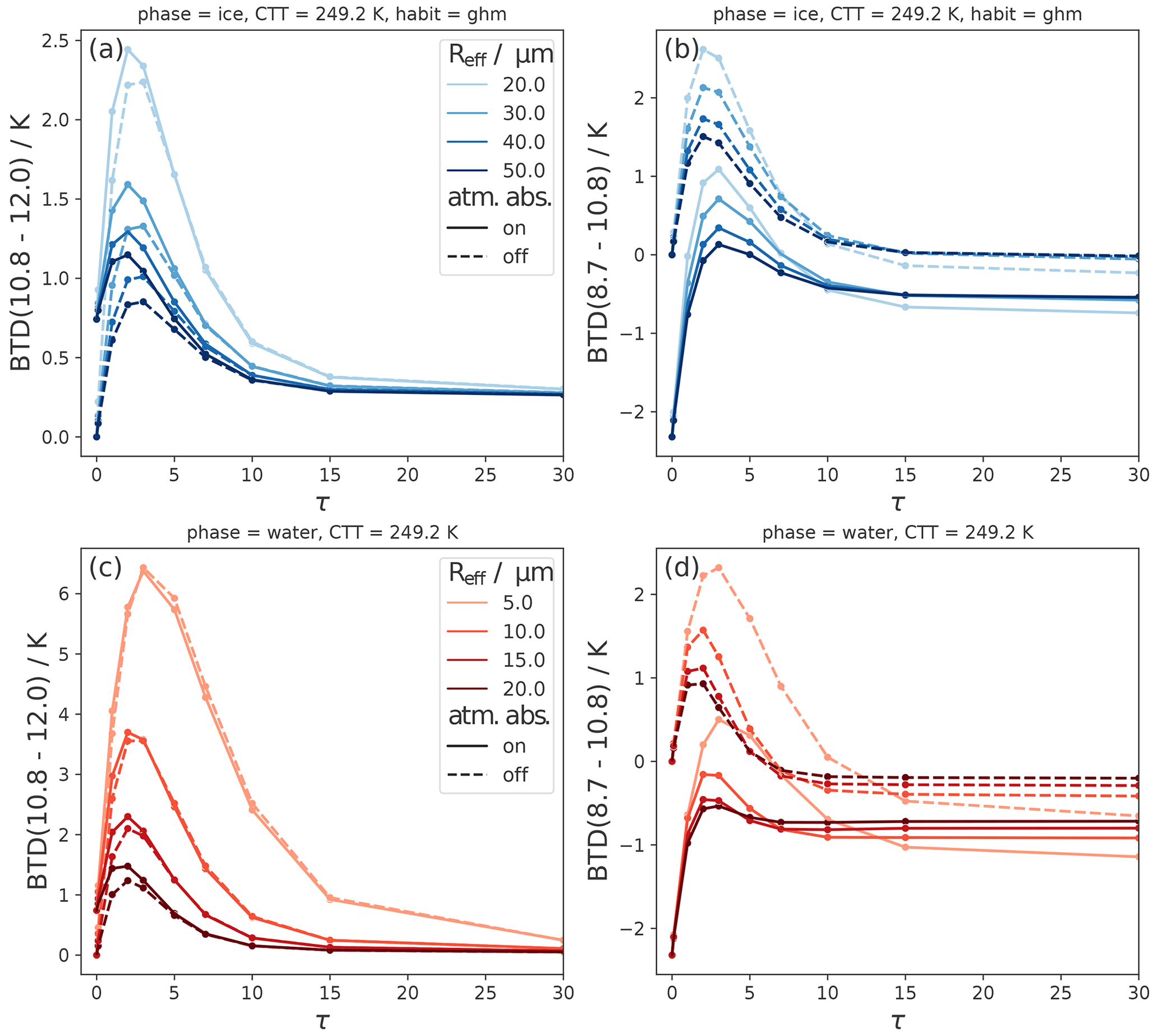
Figure 7Effects of varying Reff on BTD(10.8–12.0) and BTD(8.7–10.8) as functions of τ for ice clouds (a, b) and liquid clouds (c, d). Solid lines indicate a “normal” absorbing atmosphere, and dashed lines indicate that molecular absorption is switched off.
The effect of Reff on BTD(10.8–12.0) physically results from the dependence of particle absorption on Reff: the spectral differences of the absorption coefficient are larger for smaller Reff (see Fig. 3), resulting in lower transmission at 12.0 than at 10.8 µm and thus higher BTD(10.8–12.0) values for smaller Reff values. The effect of scattering on BTD(10.8–12.0) is similar for varying Reff and comparatively small (increases (decreases) the BTD by ⪅0.5 K for ice (water) clouds). For the interested reader, Fig. C1 shows the sensitivity of both BTDs with Reff broken down into effects of absorption and scattering.
For BTD(8.7–10.8), the Reff dependence for small τ is, like the phase dependence, the result of two opposite effects: for smaller Reff, absorption increases for 10.8 compared to 8.7 µm, leading to an increase in BTD(8.7–10.8). On the other hand, scattering increases more for 8.7 than for 10.8 µm, leading to a decrease in BTD(8.7–10.8). However, the effect due to absorption is stronger and therefore the BTD(8.7–10.8) increases with decreasing Reff. Unlike BTD(10.8–12.0), BTD(8.7–10.8) is still dependent on Reff at large τ: here BTD(8.7–10.8) increases with increasing Reff, contrary to the Reff trend at small τ. The smaller the Reff, the more important this effect becomes.
The most important insights are summarized below.
-
The BTDs depend strongly and nonlinearly on Reff.
-
Physically this dependence is due to larger spectral differences in the absorption coefficient for smaller Reff.
-
For BTD(8.7–10.8), stronger scattering for smaller Reff mediates the absorption effects.
5.5 Effects of ice crystal habit on BTDs
Figure 8 shows the sensitivity of the BTDs to ice crystal habits (in ice clouds). For both BTDs, rough aggregates lead to the smallest BTD values. For BTD(8.7–10.8), ice crystals with the general habit mix (ghm) lead to the largest BTD values, while for BTD(10.8–12.0), solid columns lead to slightly higher values. However, the sensitivity to ice crystal habits is relatively small (⪅ 0.5 K) compared to other cloud properties. This confirms the results of Dubuisson et al. (2008), who showed that the habit has a small effect on BTDs compared to the effect of Reff, also for ice crystal shapes other than the ones considered here. The relative importance of different cloud parameters will be further discussed in Sect. 6.
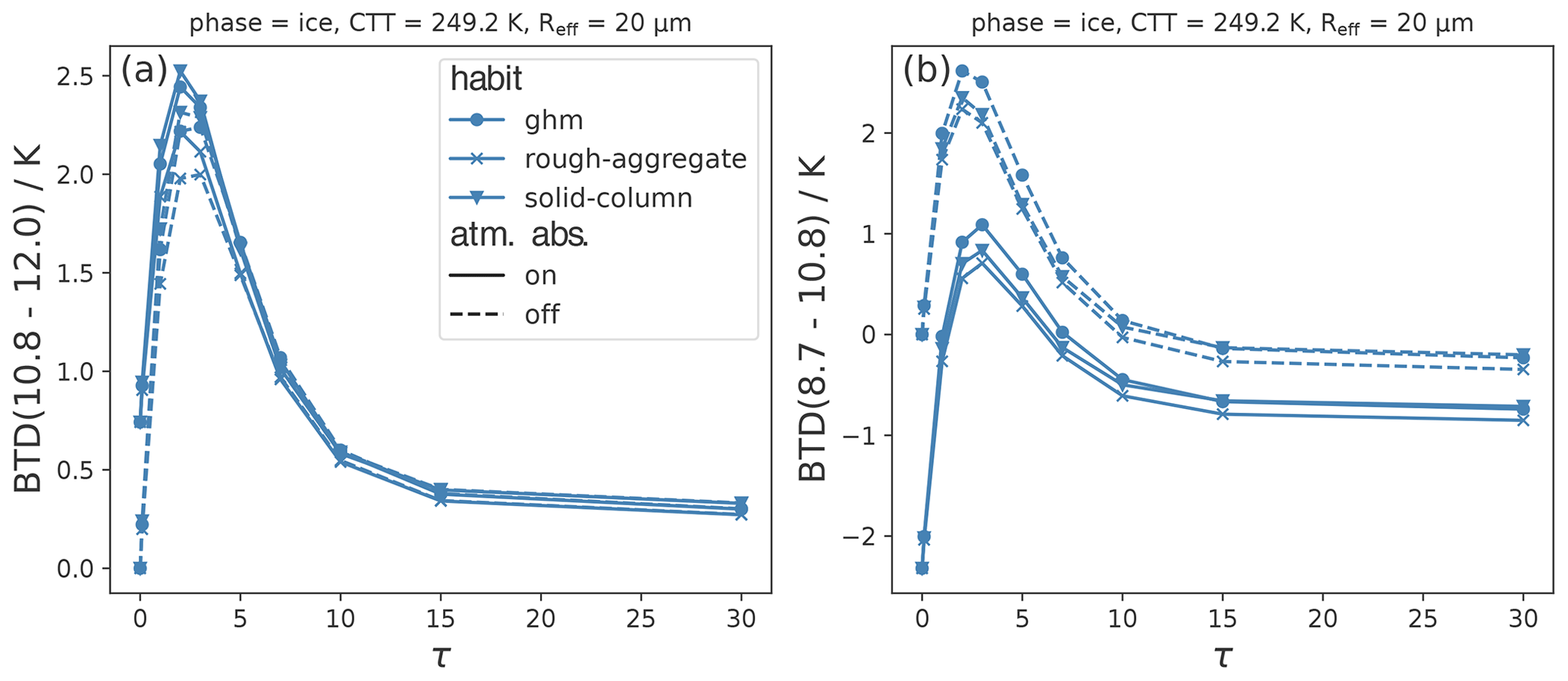
Figure 8Effects of varying ice crystal habit on (a) BTD(10.8–12.0) and (b) BTD(8.7–10.8) as functions of τ for ice clouds. Solid lines indicate a “normal” absorbing atmosphere, and dashed lines indicate that molecular absorption is switched off.
5.6 Effects of cloud-top temperature on BTDs
Figure 9 shows the sensitivity of both BTDs to CTT – and thus to CTH – for ice (top row) and liquid (bottom row) clouds. The results with molecular absorption switched off (dashed lines) show how much of this sensitivity is due to the atmosphere. Note that the CTT ranges for ice and liquid clouds are different in order to simulate realistic cloud conditions.
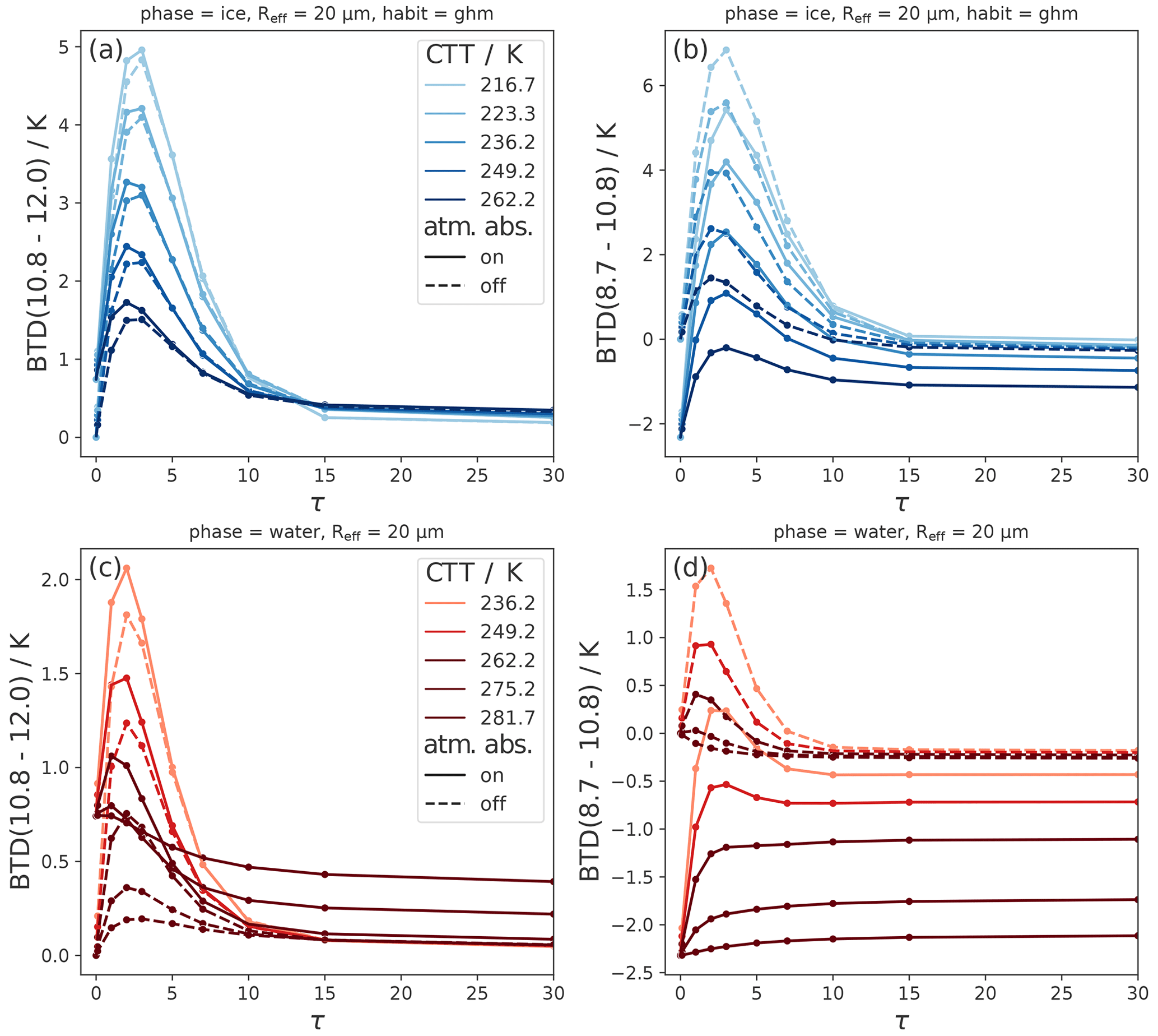
Figure 9Effects of varying cloud-top temperature (CTT) on BTD(10.8–12.0) and BTD(8.7–10.8) as a function of τ for ice clouds (a, b) and liquid clouds (c, d). Solid lines indicate a “normal” absorbing atmosphere, and dashed lines indicate that molecular absorption is switched off.
For BTD(8.7–10.8), molecular absorption is relevant for all τ values: clouds with high CTT, i.e., low CTH, have more absorbing atmosphere above cloud top, leading to more radiation absorbed at 8.7 compared to 10.8 µm. For BTD(10.8–12.0), this effect is less pronounced and molecular absorption is only relevant when there is a long path through the atmosphere (i.e., low CTH or small τ).
At low τ (⪅10), both BTD(8.7–10.8) and BTD(10.8–12.0) show a strong dependence on CTT that is not due to molecular absorption. Since the single-scattering properties are not CTT-dependent (see Sect. 2), this CTT effect on the BTDs is also not (directly) due to spectral differences in the single-scattering properties – in contrast to the effects of the other cloud parameters discussed above. Instead, there are more subtle reasons for this effect: in Sect. 4 we found that the BTD nonlinearity shift leads to a CTT dependence of the BTDs with higher BTD values for lower CTTs even when optical cloud properties are the same for all wavelengths. This explains part of the CTT dependence in Fig. 9. In Appendix B we further discuss the BTD nonlinearity shift, also allowing wavelength-dependent optical properties. It can be shown that for the Schwarzschild BTDS, spectral differences in the extinction coefficient are scaled by the difference between the surface and the cloud-top radiance, Bλ(Ts)−Bλ(CTT) (see Appendix B for a detailed discussion). Hence, the effects of spectral differences in optical properties on BTDS are amplified by larger ΔT, i.e., differences between Ts and the CTT. This is the main reason (besides the BTD nonlinearity shift) for the CTT dependence of the BTDs. Colder CTTs (or rather larger ΔT) thus increase both the BTD nonlinearity shift and the effects of spectral differences in optical properties.
The following list summarizes the CTT and CTH effects on the BTDs.
-
For BTD(8.7–10.8), CTH has a large effect due to molecular absorption mainly above cloud top.
-
Both BTDs show a strong dependence on CTT (or more generally on ΔT) with higher values for lower CTTs (larger ΔT).
-
The BTD nonlinearity shift is co-responsible for the positive BTD values and the CTT (or ΔT) dependence of the BTDs, adding to the effects stemming from spectral differences in absorption and scattering properties.
In the last section we analyzed the effects of cloud properties on the BTDs individually by varying only one cloud property at a time (besides τ). In this section we combine the phase-related cloud parameters τ, Reff, ice habit, CTT, and thermodynamic phase for a sensitivity analysis of the BTDs. From this analysis we determine typical BTD ranges for ice and liquid clouds and understand which cloud parameters are responsible for the phase information contained in the BTDs. We analyze for which cloud scenarios we can distinguish between liquid clouds and ice clouds and when they overlap, allowing us to derive implications for phase retrievals. First, in Sect. 6.1, we perform sensitivity analyses for each BTD individually. Next, in Sect. 6.2, we study the sensitivities and phase information content of the two BTDs combined.
6.1 Sensitivity analysis for each BTD
To study when BTDs can typically distinguish between liquid and ice clouds, Fig. 10 gives an overview of the sensitivities of the BTDs for “typical” cloud scenarios, as defined in the following. The figure shows the BTDs for upper and lower boundaries of CTT (217–249 K for ice, 262–282 K for liquid water) and Reff (20–50 µm for ice, 5–20 µm for liquid water). These ranges are representative for midlatitude clouds (between 30 and 50° N or S) and are chosen as follows: the CTT boundaries are derived from the active remote sensing product DARDAR (lidar/radar; Delanoë and Hogan, 2010) – specifically, values close to the 15th and 85th percentiles of ice and liquid CTTs observed for midlatitude clouds, covering about 70 % of CTTs (see Mayer et al., 2023, for detailed information on the data set). The cloud scenarios with the two CTT boundary values per phase are shown in different colors in Fig. 10 (light blue and dark blue for ice clouds; orange and red for liquid clouds). For the Reff boundaries we select the upper and lower limits of all computed Reff scenarios (see Table 1). Additionally, as liquid clouds rarely have τ<5, these values are omitted, since we focus for this sensitivity analysis on typical cloud scenarios. For ice clouds, different habits are shown as different markers. Hence, the cloud parameters in Fig. 10 are chosen such that the majority of midlatitude cloud events for each phase lie between the very bottom and top blue curves for ice and the very bottom and top orange–red curves for liquid.
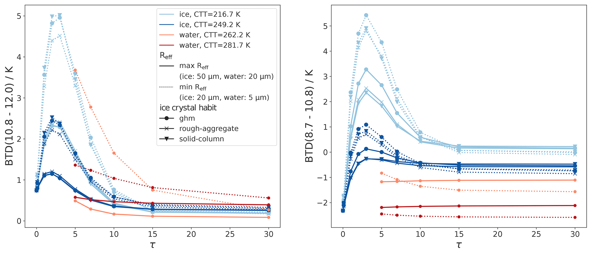
Figure 10Sensitivity analysis for each BTD varying the phase-related cloud parameters τ, Reff, habit, CTT, and thermodynamic phase: BTD(10.8–12.0) and BTD(8.7–10.8) for typical upper and lower boundaries of CTT and Reff for ice (blue colors) and liquid (orange–red colors) clouds. For ice clouds, different habits are shown as different markers. The figure shows typical BTD ranges for ice and liquid clouds.
To verify that the computed ranges of BTD values are realistic, we compare the RT results with measured SEVIRI data using cloud-phase information from DARDAR. More details on this comparison and its results can be found in Appendix D. We find good agreement between the RT results and the measured SEVIRI data and conclude that the results of the RT calculations are realistic.
In Fig. 10 BTD(10.8–12.0) shows the highest sensitivity to τ, CTT, and Reff. BTD(8.7–10.8) shows the highest sensitivity to τ, CTT, and molecular absorption (closely linked to CTH). In comparison to τ, CTT, and CTH, the sensitivity to Reff is lower for BTD(8.7–10.8) and mainly relevant for small CTT. For both BTDs, the direct sensitivity to cloud phase, i.e., holding all other cloud parameters constant, plays mostly only a minor role: for BTD(10.8–12.0) the direct phase dependence is of the order of 0.5–1.5 K; for BTD(8.7–10.8) the direct influence of phase is only significant for small τ values (⪅10) and then of the order of 1–2 K (see Sect. 5.3).
For a phase retrieval we need to know for which cloud properties liquid and ice clouds overlap and where they separate for both BTDs. The largest BTD(10.8–12.0) values in the typical cloud scenarios (about 2.5 to 5 K in Fig. 10) are only observed for optically thin and cold ice clouds with small Reff. Thus BTD(10.8–12.0) is useful to detect cirrus clouds, especially if they have small Reff (like contrails), and classify them as ice in a phase retrieval. However, our calculations show that certain liquid cloud scenarios with exceptionally low Reff and cold CTTs can also induce remarkably high BTD(10.8–12.0). This can lead to misclassification of these liquid clouds as ice. However, most liquid clouds have lower BTD(10.8–12.0), below about 2.5 K in Fig. 10. Since such low BTD(10.8–12.0) may also indicate ice clouds with “warm” CTTs and/or large Reff, or ice clouds with τ close to zero, a phase classification based on BTD(10.8–12.0) alone is challenging. The lowest BTD(10.8–12.0) values (about 0 to 1 K in Fig. 10) indicate optically thick clouds but otherwise do not contain much phase information.
As for BTD(10.8–12.0), large BTD(8.7–10.8) (around 1 to 5.5 K in Fig. 10) can indicate ice phase, since only ice clouds with low τ of about reach these values. Low BTD(8.7–10.8) (lower than about −0.5 in Fig. 10) can arise from very thin ice clouds (as BTD(8.7–10.8) decreases to about −2 K as τ goes to zero) or optically thick clouds. For optically thick clouds, BTD(8.7–10.8) decreases with higher CTT (due to lower CTHs and stronger molecular absorption) and smaller Reff – both characteristics typical of liquid clouds. As a general guideline for optically thick clouds, lower BTD(8.7–10.8) indicates a higher probability of a liquid cloud. Overall, the phase information contained in BTD(8.7–10.8) originates mainly from its sensitivity to CTT for clouds with τ⪅10, while for optically thick clouds it stems mainly from its sensitivity to molecular absorption (closely linked to CTH) and (to a lesser extent) Reff. Only in cases of optically thin clouds (τ⪅10) is the phase information of BTD(8.7–10.8) additionally due to the direct phase influence on the (different) absorption properties of liquid and ice particles.
The main findings are summarized below.
-
The sensitivities of the BTDs are complex.
-
BTD(10.8–12.0) shows the highest sensitivity to τ, CTT, and Reff. BTD(8.7–10.8) shows the highest sensitivity to τ, CTT, and CTH.
-
Thin ice clouds can be detected by both BTD(10.8–12.0) and BTD(8.7–10.8) as long as τ⪆1.
-
BTD(8.7–10.8) also provides CTH and Reff information for optically thick clouds, which can be useful for phase determination.
-
For BTD(10.8–12.0), typical liquid and ice clouds overlap for most cloud scenarios, with the exception of cold, thin ice clouds. For BTD(8.7–10.8), liquid and ice clouds separate better, but the BTD values of the two phases are close when CTTs (CTHs) are similar. This phase separation is mainly due to the sensitivity of BTD(8.7–10.8) to CTT and CTH.
6.2 Sensitivity analysis for the combination of both BTDs
We perform a similar sensitivity analysis as in the last section for the combination of both BTDs. As in Fig. 10, Fig. 11 shows the BTDs for the same upper and lower boundaries of CTT and Reff but in the space spanned by BTD(8.7–10.8) and BTD(10.8–12.0). Along each line, τ increases from 0 to 30. To make the shape of the curves easier to understand, here liquid clouds with τ<5 are also shown (in contrast to Fig. 10).
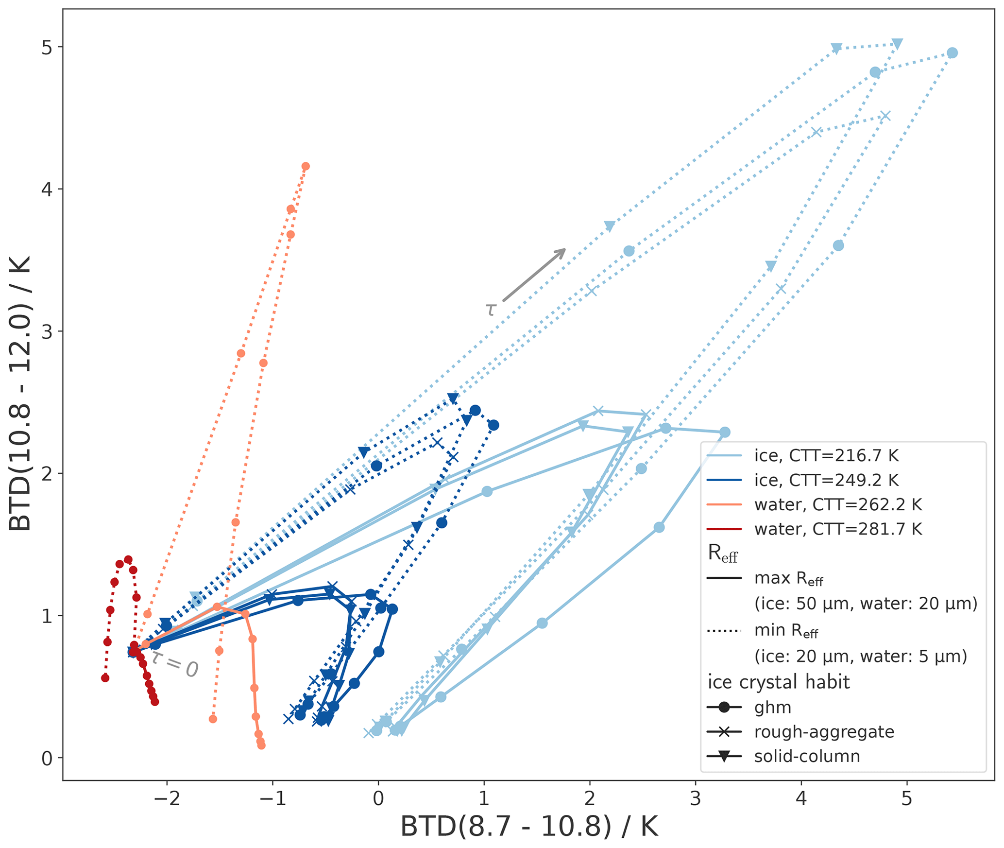
Figure 11Sensitivity analysis combining both BTDs and varying the cloud parameters τ, Reff, habit, CTT, and thermodynamic phase: blue lines show ice clouds, and orange–red lines show liquid clouds for typical upper and lower boundaries of CTT and Reff. Along each line, τ increases from 0 to 30. For ice clouds, different habits are shown as different markers.
Figure 11 shows that the combined knowledge of both BTD(8.7–10.8) and BTD(10.8–12.0) leads to a better phase classification than considering BTD(8.7–10.8) and BTD(10.8–12.0) individually. For instance, liquid clouds at cold CTTs and small Reff (orange dotted line) separate from ice clouds in Fig. 11 as long as τ is not too large (⪅10). In contrast, the same cloud scenario overlaps with ice cloud scenarios when only BTD(8.7–10.8) or BTD(10.8–12.0) is considered individually (Fig. 10).
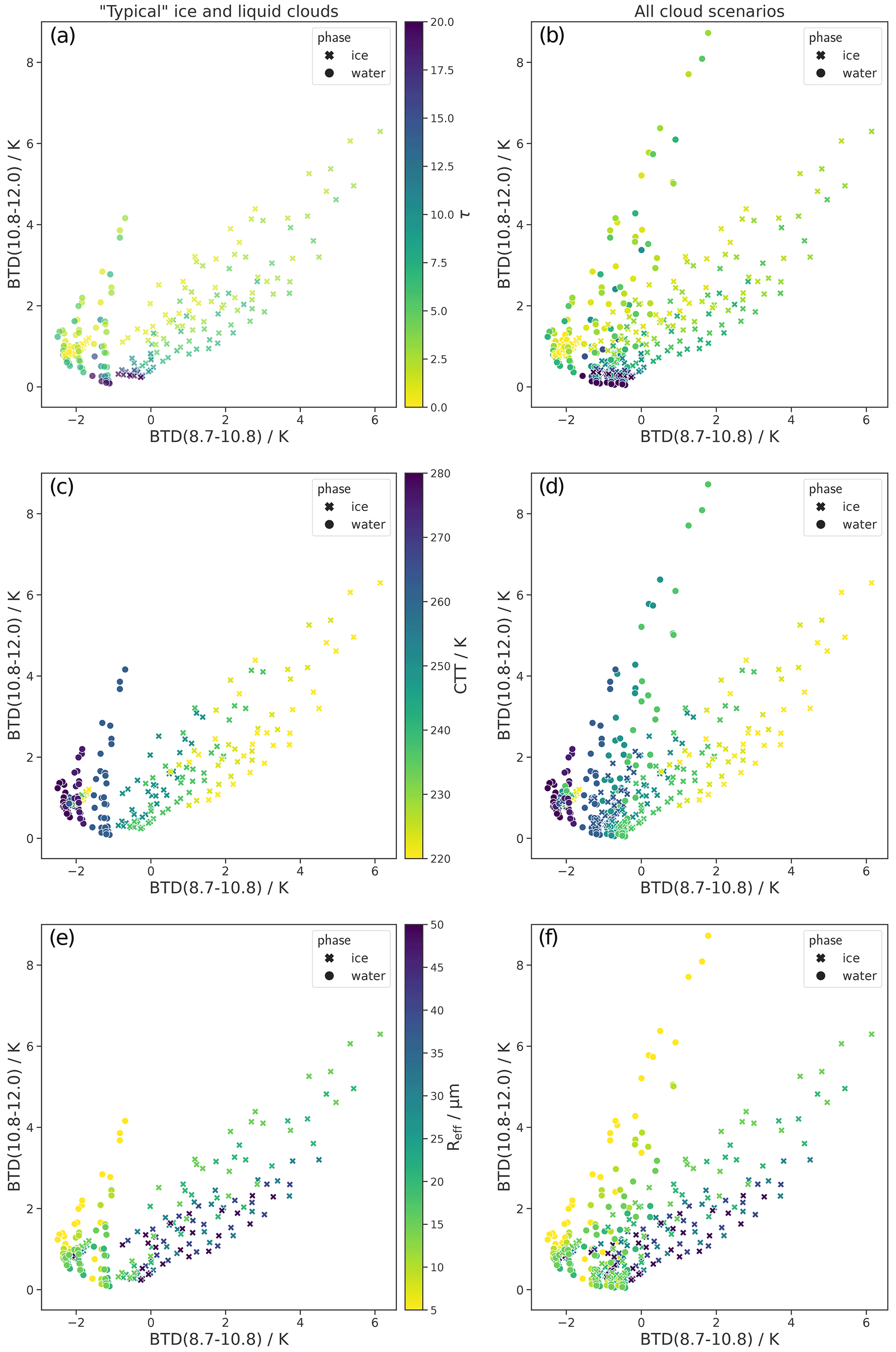
Figure 12Left column (a, c, e): BTD(10.8–12.0) and BTD(8.7–10.8) values within the defined “typical” boundaries of CTT. Round markers indicate liquid clouds; crosses indicate ice clouds. Clouds which can be distinguished using a CTT proxy like BT10.8, i.e., optically thick clouds (τ≥10) with very low (<233 K) or very high (>273 K) CTTs, are not shown. The color code in the three rows encodes τ, CTT, and Reff, respectively. Right column (b, d, f): same as left column but for the whole range of computed cloud scenarios (see Table 1), also including exceptionally cold liquid clouds and exceptionally warm ice clouds. The color codes of the three rows correspond to the color codes in the left column. Clouds which can be distinguished using a CTT proxy are again not shown.
In order to better showcase the range of BTD values for both phases and identify overlap regions, we use an additional type of plot: instead of showing only the boundary cases (as in Fig. 11), the left column of Fig. 12 shows (almost) all computed BTD values within the defined boundaries of CTT and Reff in the space spanned by the two BTDs. Only optically thick clouds (τ≥10) with very low (<233 K) or very high (>273 K) CTTs are removed, i.e., the clouds that are easily categorized as liquid or ice by a CTT proxy such as BT10.8 and for which a categorization by the BTDs is therefore not necessary. Liquid clouds are shown as round markers, while ice clouds are shown as crosses. The three panels in the left column of Fig. 12 vary only by their color code, which encodes τ, CTT, and Reff, respectively. They show that there is little overlap between the typical liquid and ice clouds (i.e., the clouds within the defined CTT and Reff boundaries). The only overlap is for very small τ (τ⪅1), since the BTDs approach the same values for all clouds, determined by atmospheric properties, as τ→0 (best seen in Fig. 11). This means that a phase classification for typical liquid and ice cloud cases is possible in BTD(8.7–10.8)–BTD(10.8–12.0) space for τ⪆1 when atmospheric parameters are known.
However, Fig. 11 and the left column in Fig. 12 also show that liquid and ice BTD values are closest for clouds with similar CTTs. To further explore this issue and to test the limitations of a phase classification using the BTDs, the right column of Fig. 12 also shows BTD values for clouds outside the typical cloud boundaries. The three panels show the whole range of computed cloud scenarios (see Table 1), also including exceptionally cold liquid clouds and exceptionally warm ice clouds. Only the “easy” to distinguish cases (τ≥10 and either CTT<233 K or CTT>273 K) are removed as before. The figures show that the overlap between liquid and ice clouds is significantly larger compared to the typical cloud cases (left column of Fig. 12). The clouds in the overlap region are mainly liquid and ice clouds which have similar CTTs in the mid-level temperature range, i.e., rather cold liquid clouds (CTT⪅260 K) and rather warm ice clouds (CTT⪆250 K). We discussed in the last section (Sect. 6.1) that the CTT (and the closely linked CTH) is the most important contributor to the differences between liquid and ice clouds for both BTDs. It is therefore not surprising that phase discrimination for clouds with similar CTT is difficult even when knowledge of both BTDs is combined. Also note that additional information from BT10.8, which is often used as a proxy for CTT, does not help much in distinguishing between phases in these cases of mid-level CTTs. For the phase classification of these mid-level clouds, the Reff also plays a role: for Reff values that are rather large for the respective phase, the overlap occurs for all τ values; for Reff values that are rather small for the respective phase, the overlap occurs only for very small or very large τ values.
The most important results are summarized below.
-
The combined use of BTD(8.7–10.8) and BTD(10.8–12.0) is better suited for phase discrimination than the two BTDs individually.
-
The combined use of BTD(8.7–10.8) and BTD(10.8–12.0) can discriminate cloud phase for liquid and ice clouds in their typical CTT regimes as long as τ is not too small (τ⪆1) and when atmospheric parameters are known.
-
Clouds in the mid-level CTT regime are challenging: if liquid clouds are particularly cold or ice clouds particularly warm, they often cannot be distinguished by the two BTDs. This is especially true for clouds with large Reff for the respective phase.
6.3 Sensitivity to additional cloud parameters: effects of geometric thickness and vertical Reff inhomogeneity
Cloud properties that have not been discussed so far are cloud geometric thickness and vertical inhomogeneities of microphysical parameters. Both can have an impact on BTDs (Piontek et al., 2021a; Zhang et al., 2010). To estimate how large these effects are, we performed a sensitivity analysis for varying cloud geometric thickness and for vertical inhomogeneities of Reff. Results of this analysis are shown in Figs. E1 and E2. We find that the sensitivity to both geometric thickness and vertical Reff inhomogeneity is small compared to other cloud parameters (⪅0.5 K in most cases). This sensitivity does not significantly affect the regions in the space spanned by the two BTDs which are associated with the different phases and therefore has a comparatively small effect on a potential phase retrieval.
The aim of this study is to characterize and physically understand the relation of two IR window BTDs that are typically used for satellite retrievals of the thermodynamic cloud phase. As an example, we select BTD(8.7–10.8) and BTD(10.8–12.0) from SEVIRI, but the main findings can be generalized to other imagers with similar thermal channels. Although modern phase retrievals often rely not only on BTDs but also on other satellite measurements (Baum et al., 2012; Hünerbein et al., 2023; Benas et al., 2023; Mayer et al., 2024), it is important to understand the BTD characteristics and capabilities. This knowledge helps to design optimal cloud-phase retrievals and to understand their potential and limitations.
We present RT calculations that analyze the sensitivities of the two BTDs to cloud phase and all radiatively important cloud parameters related to phase, namely τ, Reff, ice crystal habit, CTT, and CTH. Previous studies of BTDs have tended to focus on only a small number of cloud parameters, and an overview of the relative importance of all cloud parameters and their interdependencies is still missing. We perform a sensitivity analysis of the BTDs, which to our knowledge has never been done for all cloud parameters combined. This provides an overview of the effects of all cloud parameters and shows which parameters are responsible for the observed phase dependence of the BTDs, which is often used for phase retrievals (Ackerman et al., 1990; Strabala et al., 1994; Finkensieper et al., 2016; Key and Intrieri, 2000; Baum et al., 2000, 2012; Hünerbein et al., 2023; Benas et al., 2023; Mayer et al., 2024). Even though the RT calculations were performed for a specific atmospheric and surface setup, the main insights of this study, including the physical understanding of the effects of cloud properties on BTDs and their relative importance, are valid for any atmospheric or surface condition.
To understand the behavior of the BTDs, we examine the effects of the nonlinear relationship between radiances and BTs through Planck's radiation law on the BTDs. This nonlinearity induces positive BTD values and a dependence on the CTT (or more generally the surface–cloud temperature contrast ΔT) in a simple RT model, even when cloud optical properties (transmittance and emissivity) are the same at all wavelengths. This effect is co-responsible for the arc shape of the BTDs as functions of τ and their CTT dependence, in addition to effects due to spectral differences in cloud optical properties. These spectral differences in cloud optical properties can explain the (remaining) dependence of the BTDs on the different cloud parameters.
We find that the dependence on phase is more complex than is sometimes assumed: although both BTDs are directly sensitive to phase (holding every other cloud parameter constant), this sensitivity is mostly small compared to other cloud parameters, such as τ, CTT, and Reff. Instead, apart from τ for which the sensitivity is well known, the BTDs show the strongest sensitivity to CTT (and the closely linked CTH). Since the CTT is associated with phase, this is the main factor leading to the observed phase dependence of the BTDs. Note that more generally, this CTT dependence of the BTDs is more accurately described as a dependence on the surface–cloud temperature contrast ΔT, which reduces to a CTT dependence in our case with a fixed surface temperature. The direct phase dependence merely adds to the CTT effect, increasing differences between ice and liquid (for BTD(8.7–10.8) only for small τ⪅10).
The sensitivity analysis shows that it is straightforward to distinguish typical high ice clouds from low liquid clouds using the BTDs. However, it is challenging to distinguish a mid-level ice cloud from a mid-level liquid cloud – especially if the Reff is also similar. The combination of both BTDs increases phase information content and is therefore preferable in a retrieval.
This study was conducted for a simple fixed setup of the atmosphere, surface, and satellite viewing geometry in order to focus on the effects of cloud properties. If this setup is changed, we expect the cloud effects on the BTDs discussed in this paper to be superimposed by additional effects: for example, changes in water vapor content or satellite zenith angle shift BTD(8.7–10.8) due to its sensitivity to water vapor absorption. This shift is larger the more water vapor is above the cloud top and therefore depends on the CTH and the vertical atmospheric profile. A different type of surface with spectral differences in surface emissivity (for instance, a desert surface) shifts the values of both BTDs for optically thin clouds. For potential phase retrievals, these effects should ideally be taken into account.
This study focuses on liquid and ice clouds. We expect the BTD values of mixed-phase clouds to lie between ice and liquid values, as they represent a transition between the two. Depending mainly on the CTT and CTH, and to a lesser extent the Reff of mixed-phase clouds, their BTD values are expected to be closer to or further away from the liquid or ice BTD values. In that sense, we expect that BTDs can make a useful contribution to the retrieval of mixed-phase clouds and their composition. However, as the CTT, CTH, and Reff values overlap between liquid, mixed-phase, and/or ice clouds, we expect the regions of the different phases in the space spanned by BTD(8.7–10.8) and BTD(10.8–12.0) to also overlap, introducing ambiguity. The use of additional satellite channels containing, for instance, particle size or phase information is necessary to increase the phase information content for a retrieval.
The single-scattering properties are the volume extinction coefficient βext, the single-scattering albedo ω0, and the scattering phase function p. The volume extinction coefficient βext describes how much radiation is removed through scattering and absorption (extinction) from a ray when passing through the cloud and can be expressed as
where βsca and βabs are the scattering and absorption coefficient, with units of m−1, measuring how much radiation is absorbed and scattered by cloud particles. Note that in this study τ is βext at wavelength λ=550 nm integrated over the path through the cloud; the optical thickness τλ at other wavelengths λ is in general different from τ, depending on the other microphysical cloud parameters. The single-scattering albedo ω0 is a measure of the relative importance of scattering and absorption, defined as
Hence, as an alternative to βext and ω0 one can equivalently describe radiative transfer by βabs and βsca, which can be easier to interpret. The scattering phase function p(Ω) gives the probability of the scattering angle Ω, i.e., the angle between the incident radiation and the scattered radiation. To understand radiative transfer through a cloud, the most important property of p is the angular anisotropy of the scattering process. This anisotropy is indicated to first order by the asymmetry parameter g, which is calculated from p as the mean cosine of the scattering angle Ω.
If a particle scatters more in the forward direction (Ω=0°), g is positive; g is negative if the scattering is more in the backward direction (Ω=180°) (Bohren and Huffman, 2008).
An instructive way to look at the BTD nonlinearity shift and to disentangle it from effects of wavelength-dependent optical properties is the following: to make the radiances at different wavelengths more comparable, we use the Planck radiance corresponding to the surface temperature Ts as a reference. For typical atmospheric profiles (without temperature inversions), this Planck radiance Bλ(Ts) is the maximal possible radiance in each wavelength, corresponding to τ→0 (see Eq. 3). We express the TOA radiance as fractions fλ of this maximal possible radiance, called radiance fraction in the following, i.e.,
The BTDs can then be expressed as functions of the radiance fractions fλ:
For the sake of brevity, in the following we only discuss BTD(8.7–10.8) as a function of f8.7 and f10.8; BTD(10.8–12.0) qualitatively has the same properties and the same conclusions apply. Figure B1 shows BTD(8.7–10.8) in f8.7–f10.8 space for Ts=290 K. If f8.7 is (much) larger than f10.8, the BTD is positive, and if f8.7 is (much) smaller than f10.8, the BTD is negative, as expected. However, the BTD(8.7–10.8)=0 line is not at f8.7=f10.8 (black dashed line in Fig. B1) as one might naively expect but has a convex shape in f8.7–f10.8 space (shown as a solid black line) such that BTD(8.7–10.8)=0 for f8.7<f10.8. Or to put it another way, if the radiance at TOA is the same fraction of its maximal possible radiance at both wavelengths, f8.7=f10.8, the BTD is positive. Note that this is a completely general statement that does not depend on an RT model but simply shows what happens mathematically when the inverse Planck function, Tλ, is applied to fractions of Planck radiance, fλBλ(Ts), at different wavelengths.
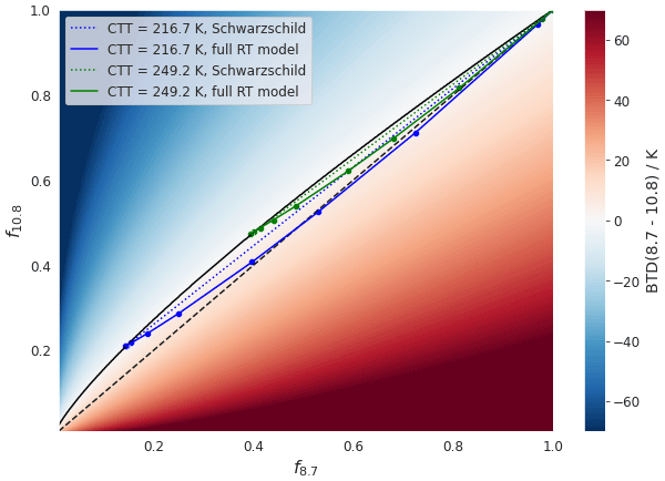
Figure B1BTD(8.7–10.8) in the space spanned by the radiance fraction f8.7 and f10.8 (defined as the radiance at TOA scaled by the Planck radiance of the surface with temperature Ts=290 K: ). The solid black line indicates BTD(8.7–10.8)=0; the dashed black line indicates f8.7=f10.8. The blue and green lines show f8.7 and f10.8 values for varying τ at a given CTT: the dotted lines show f8.7 and f10.8 computed with the Schwarzschild equation (with τ8.7=τ10.8), and the solid lines show f8.7 and f10.8 values computed with the full RT model.
To understand the role of the BTD nonlinearity shift we add results of RT computations to Fig. B1 in the following steps: first, we study how radiances computed with the Schwarzschild equation look in f8.7–f10.8 space. To see the pure BTD nonlinearity shift we again set the optical thickness as constant at both wavelengths, . Next, we explore the changes in the Schwarzschild radiance when τ differs at the two wavelengths, i.e., τ10.8≠τ8.7. In this case, both the mathematical BTD nonlinearity shift and the physical effect of spectrally dependent optical properties are present. Third, we study how the radiance computed with the full RT model looks in f8.7–f10.8 space.
We start with the Schwarzschild radiance in f8.7–f10.8 space with constant optical thickness at both wavelengths, . We compute the radiances and from the Schwarzschild equation as functions of τ for different values of CTT, as before (see Fig. 4b). These radiance results, expressed as radiance fractions f8.7 and f10.8, are shown in Fig. B1 as dotted lines for two different CTTs. For τ=0, the TOA radiance is the radiance emitted by the surface and . As τ increases, f8.7 and f10.8 get smaller and BTD(8.7–10.8)>0, since f10.8 and f8.7 show a linear relationship and the BTD(8.7–10.8)=0 line is convex. For large τ (τ=30) the TOA radiance approaches the radiance emitted by a black body with a temperature equal to the CTT. Hence, the radiance fractions for large τ depend on the CTT and lie on the BTD(8.7–10.8)=0 line (see Fig. B1). Overall, for increasing τ from 0 to 30, the Schwarzschild radiance fractions form a line from to the radiance fraction values corresponding to the CTT black-body radiance. It follows from the convex shape of the BTD(8.7–10.8)=0 line that lower CTTs lead to larger BTD(8.7–10.8) values (see Fig. B1). The fact that the Schwarzschild radiance fraction line deviates from the BTD(8.7–10.8)=0 line such that BTD(8.7–10.8)>0, depending on the CTT, is a representation of the BTD nonlinearity shift equivalent to Fig. 4b. The property that f10.8 is a linear function of f8.7 can be shown from the Schwarzschild equation. Solving Eq. (3) for e−τ for a given wavelength λ0 and inserting it into the Schwarzschild equation for a second wavelength λ1 gives
with
i.e., a linear relationship between and and therefore also between and .
So far we have set τ constant for all wavelengths in the Schwarzschild equation. To see what happens in the Schwarzschild model for different τ at different wavelengths, i.e., , we add a small perturbation to ,
Since the Schwarzschild equation neglects scattering, τλ is determined by the absorption coefficient βabs,λ and the cloud water path. For λ1=10.8 µm and λ0=8.7 µm, the absorption coefficients , meaning that if scattering is neglected τ8.7<τ10.8 and δτ>0 for this case. Solving Eq. (3) for a given λ0 analog to above for and inserting into Eq. (3) for λ1 gives
where we used . Hence, since δτ>0 for λ1=10.8 µm and λ0=8.7 µm, decreases when we add a perturbation . This makes physical sense, since a larger τ10.8 compared to τ8.7 means that less radiance is transmitted through the cloud at 10.8 compared to 8.7 µm. The amount by which decreases is determined by the difference between surface and cloud-top radiance, , and the factor . For , meaning that the cloud water path approaches zero, δτ→0. For large , . Hence, the last term in Eq. (B7) vanishes for very small or large . For the values in between, the perturbation δτ leads to a decrease in and therefore in f10.8. As a result, the Schwarzschild radiance fraction line in f8.7–f10.8 space deviates from a linear to a concave line. This deviation is stronger for larger δτ (i.e., larger differences between τ10.8 and τ8.7), as well as for larger differences between the surface and the cloud-top radiance, .
As a last step of this analysis, we study the full RT model in f8.7–f10.8 space. Recall that in the full RT model, in general, , where τ as usual refers to the optical thickness at 550 nm. Figure B1 shows the radiance fractions f8.7 and f10.8 computed with the full RT model for an ice cloud for varying τ and two different CTTs as solid blue and green lines. Molecular absorption is switched off for these examples. Note that this is an equivalent representation of BTD(8.7–10.8) to the corresponding CTT curves in Fig. 9. For increasing τ from 0 to 30, the radiance fractions of the full RT model form curves from to the radiance fraction values corresponding to the black-body radiance of their CTT. These curves are concave, as expected from our theoretical considerations above (see Eq. B7). This concave shape, as explained above, can be attributed to differences in the absorption coefficients of the two wavelengths, . The concave shape results in higher BTD values compared to the Schwarzschild BTDS values, where (compare BTD(8.7–10.8) along the solid and dotted lines in Fig. B1). The figure also shows that the deviation from the linear Schwarzschild radiance fraction lines is larger for lower CTTs – in accordance with our theoretical considerations (see Eq. B7).
This leads to the following interpretation of Fig. B1: the Schwarzschild radiance fraction lines in Fig. B1 (dotted lines) represent the pure BTD nonlinearity shift, which induces positive BTD values even though τ is the same at all wavelengths. Adding spectral differences between the cloud optical properties “pushes” the radiance fraction lines into a concave shape and further increases BTD. Hence, the difference between the BTD(8.7–10.8)=0 line and the Schwarzschild radiance fraction lines in Fig. B1 is due to the nonlinearity of the transformation from radiances to BTs; the difference between the Schwarzschild radiance fraction lines and the full RT model (solid lines) in Fig. B1 is due to the spectral differences in cloud optical properties. Lower CTTs increase both the BTD nonlinearity shift and the effects of spectral differences between the cloud optical properties.
Figure C1 shows the sensitivity of both BTDs with Reff broken down into effects of absorption and scattering. The two rows show the same cloud scenarios, once with scattering switched off (top row) and once with scattering switched on (bottom row). The figure shows that the effects of absorption lead to increasing values for smaller Reff for both BTDs (top row of Fig. C1).
For BTD(10.8–12.0), the effect of scattering is similar for varying Reff and comparatively small (increases (decreases) BTD(10.8–12.0) by ⪅0.5 K for ice (water) clouds; compare Fig. C1a and b with e and f). For BTD(8.7–10.8), scattering effects are stronger than for BTD(10.8–12.0) and depend on Reff: scattering leads to a stronger decrease in BTD(8.7–10.8) for smaller Reff (compare Fig. C1c and d with g and h). Since, however, the absorption effects are stronger, BTD(8.7–10.8) increases with decreasing Reff (Fig. C1g and h).
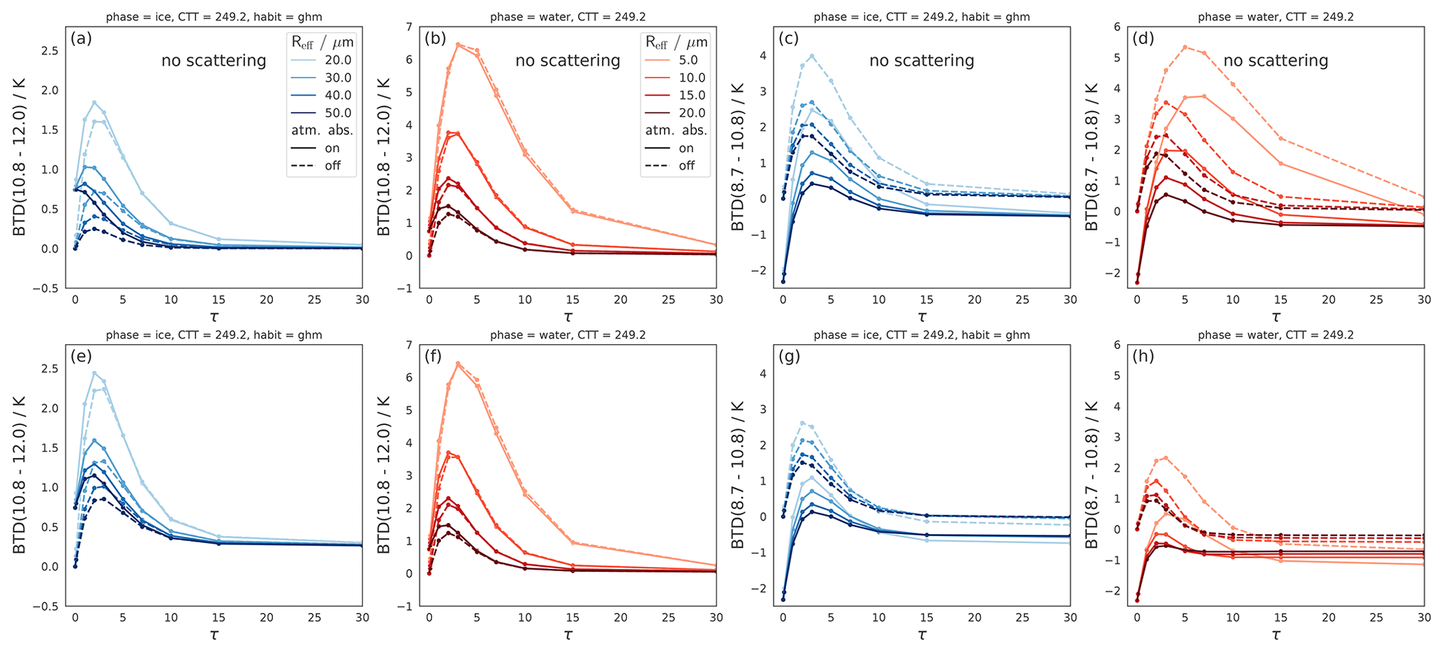
Figure C1Effects of varying Reff on BTD(10.8–12.0) and BTD(8.7–10.8) as functions of τ for ice clouds (blue) and liquid clouds (orange–red) with scattering switched off (a–d) and switched on (e–h). Solid lines indicate a “normal” absorbing atmosphere, and dashed lines indicate that molecular absorption is switched off.
Figure D1 shows a comparison of the RT results with measured SEVIRI data. The SEVIRI data were collocated with the active satellite product DARDAR (Delanoë and Hogan, 2010) containing information on the cloud phase (for more details see Mayer et al., 2023). The plot on the left shows ice clouds; the plot on the right water clouds. As in Sect. 6.1 and 6.2, the RT results show boundary cases of typical cloud scenarios in blue and red, as indicated in the legend. In addition to SATZ=0°, we also show the RT results for SATZ=50° in order to be able to compare the RT results to a large number of measurements with angles between these two cases. The measured SEVIRI data with the corresponding constraints (i.e., data for ice or water clouds within CTT and SATZ boundaries as for the RT calculations) are plotted on top of the RT results in gray. The figure shows that the RT results and measured SEVIRI data have a large overlap. Hence, the computed ranges of BTD values are realistic.
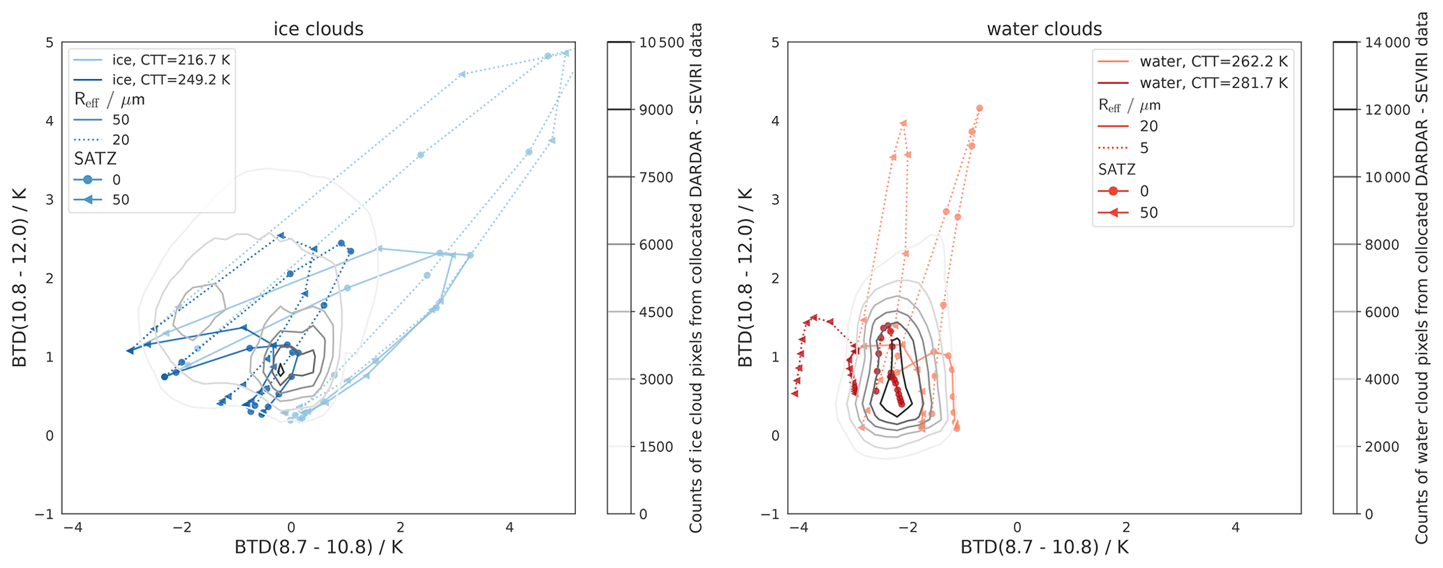
Figure E1 shows a sensitivity analysis for varying cloud geometric thickness between 1 and 4 km. For constant τ, a larger cloud geometric thickness means that radiation originates from deeper within the cloud (in terms of geometric depth, implying a larger temperature difference). This depth can differ for different wavelengths, leading to a dependence of BTDs on geometric thickness (Piontek et al., 2021a). Figure E1 shows that the sensitivity to geometric thickness is comparably small and mostly ⪅0.5 K. Exceptions are liquid clouds with very small Reff for BTD(10.8–12.0), where the sensitivity to geometric thickness can exceed 1 K. For the case of liquid clouds with CTT=281.7 K the CTH is at an altitude of 1 km in the US standard atmospheric profile. Geometric thicknesses >1 km are therefore not possible in this case.
Figure E2 shows the sensitivity of the BTDs to vertical inhomogeneity of Reff. To model this inhomogeneity and capture its basic effects on BTDs we use a simple setup of clouds with a total geometric thickness of 2 km, consisting of two 1 km thick layers (layer 1 on top, layer 2 at the bottom, specified in the subscripts). Both layers have the same optical thickness, . Cloud layer 1 has Reff,1 which is either equal to, smaller than, or larger than layer 2, Reff,1⪋Reff,2 (case A, B, or C) such that the average is the same for all three cases (case A: ; case B: ; case C: ). Hence, in case A, the Reff is homogeneous; in cases B and C it is inhomogeneous. This model of vertical inhomogeneity is of course very simplified, but it is useful for calculating a rough estimate of the magnitude of inhomogeneity effects and for understanding the underlying physics.
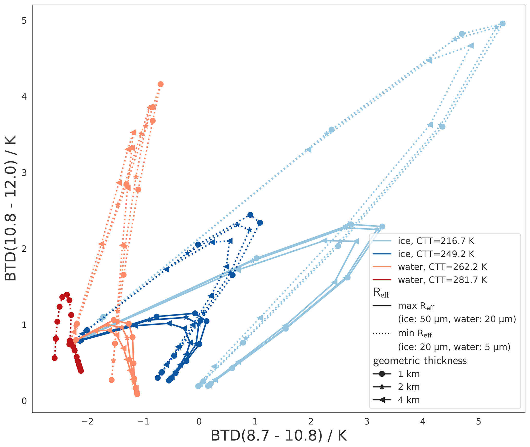
Figure E1Same as Fig. 11, but for a fixed ice crystal habit (ghm) and varying geometric thickness of the cloud (in different markers).
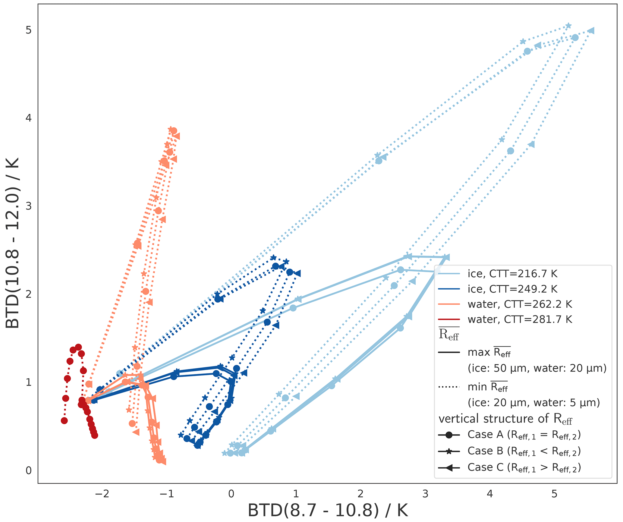
Figure E2Same as Fig. 11, but for a fixed ice crystal habit (ghm) and vertical inhomogeneity of Reff (in different markers): the cloud consists of two layers (layer 1 on top, layer 2 at the bottom, specified in the subscripts), each with a geometric thickness of 1 km and the same layer optical thickness, . Cloud layer 1 has Reff,1 which is either equal to, smaller than, or larger than layer 2, Reff,1⪋Reff,2 (case A, B, or C) such that the average is the same for all three cases (case A: ; case B: ; case C: ). No Reff inhomogeneity is shown for the case of liquid clouds with CTT=281.7 K, since their CTH is at an altitude of 1 km, leaving room for only one cloud layer.
Overall, the sensitivity to vertical Reff inhomogeneity is comparatively small (⪅0.5 K). The effects of the vertical Reff inhomogeneity on the BTDs are due on the one hand to its effects on the transmittance of the surface radiance and on the other hand to its effects on the emittance of the cloud itself. Zhang et al. (2010) show (for ice clouds) that the nonlinear dependence of the optical properties on Reff leads to an increased weighting of small particles in the signal of the transmitted radiance. This leads to larger BTDs for cases where the cloud is (partly) composed of particles smaller than the average (the inhomogeneous cases B and C), where transmittance is the dominant process (small τ). However, as can be seen in Fig. E2 for small τ (⪅2), this effect is very small compared to other dependencies, since the cloud transmittance in the infrared window depends mainly on τ and less on the details of the vertical Reff profile of the cloud (Zhang et al., 2010). On the other hand, when the cloud emittance dominates for increasing τ, the signal from the particles at the bottom of the cloud is (partially) absorbed by the top cloud layer. The BTD signal is then dominated by the Reff of the top cloud layer (Reff,1). This makes a difference mainly for small Reff values (see min curves in Fig. E2), as the BTDs depend nonlinearly on Reff (see Fig. 7). Figure E2 shows that these vertical Reff inhomogeneity effects on cloud emittance (dominant for large τ) lead to larger overall effects on the BTDs compared to the effects on transmitted surface radiance (dominant for small τ).
The libRadtran software used for the radiative transfer simulations is available from http://www.libradtran.org (last access: 22 August 2024; Mayer and Kylling, 2005; Emde et al., 2016).
All authors contributed to the project through discussions. JM carried out the simulations and the analysis of the data with valuable feedback from LB, BM, and RM. LB and CV supervised the project and provided scientific feedback. JM took the lead in writing the manuscript. All authors provided feedback on the manuscript.
The contact author has declared that none of the authors has any competing interests.
Publisher's note: Copernicus Publications remains neutral with regard to jurisdictional claims made in the text, published maps, institutional affiliations, or any other geographical representation in this paper. While Copernicus Publications makes every effort to include appropriate place names, the final responsibility lies with the authors.
We thank Klaus Gierens for constructive discussions and valuable feedback. This research was funded by the Deutsche Forschungsgemeinschaft (DFG, German Research Foundation) – TRR 301 – project ID 428312742.
This research has been supported by the Deutsche Forschungsgemeinschaft (grant no. TRR 301, project ID 428312742).
The article processing charges for this open-access publication were covered by the German Aerospace Center (DLR).
This paper was edited by Andrew Sayer and reviewed by two anonymous referees.
Ackerman, S. A., Smith, W. L., Revercomb, H. E., and Spinhirne, J. D.: The 27–28 October 1986 FIRE IFO Cirrus Case Study: Spectral Properties of Cirrus Clouds in the 8–12 µm Window, Mon. Weather Rev., 118, 2377–2388, https://doi.org/10.1175/1520-0493(1990)118<2377:TOFICC>2.0.CO;2, 1990. a, b, c
Anderson, G., Clough, S., Kneizys, F., Chetwynd, J., and Shettle, E.: AFGL atmospheric constituent profiles (0–120 km), Tech. Rep. AFGL-TR-86-0110, Air Force Geophys. Lab., Hanscom Air Force Base, Bedford, Mass., 1986afgl.rept.....A, 1986. a
Atkinson, J. D., Murray, B. J., Woodhouse, M. T., Whale, T. F., Baustian, K. J., Carslaw, K. S., Dobbie, S., O'Sullivan, D., and Malkin, T. L.: The importance of feldspar for ice nucleation by mineral dust in mixed-phase clouds, Nature, 498, 355–358, https://doi.org/10.1038/nature12278, 2013. a
Baum, B. A., Soulen, P. F., Strabala, K. I., King, M. D., Ackerman, S. A., Menzel, W. P., and Yang, P.: Remote sensing of cloud properties using MODIS airborne simulator imagery during SUCCESS: 2. Cloud thermodynamic phase, J. Geophys. Res.-Atmos., 105, 11781–11792, https://doi.org/10.1029/1999jd901090, 2000. a, b, c, d, e
Baum, B. A., Yang, P., Heymsfield, A. J., Schmitt, C. G., Xie, Y., Bansemer, A., Hu, Y.-X., and Zhang, Z.: Improvements in Shortwave Bulk Scattering and Absorption Models for the Remote Sensing of Ice Clouds, J. Appl. Meteorol. Clim., 50, 1037–1056, https://doi.org/10.1175/2010JAMC2608.1, 2011. a, b, c
Baum, B. A., Menzel, W. P., Frey, R. A., Tobin, D. C., Holz, R. E., Ackerman, S. A., Heidinger, A. K., and Yang, P.: MODIS Cloud-Top Property Refinements for Collection 6, J. Appl. Meteorol. Clim., 51, 1145–1163, https://doi.org/10.1175/JAMC-D-11-0203.1, 2012. a, b, c, d
Benas, N., Solodovnik, I., Stengel, M., Hüser, I., Karlsson, K.-G., Håkansson, N., Johansson, E., Eliasson, S., Schröder, M., Hollmann, R., and Meirink, J. F.: CLAAS-3: the third edition of the CM SAF cloud data record based on SEVIRI observations, Earth Syst. Sci. Data, 15, 5153–5170, https://doi.org/10.5194/essd-15-5153-2023, 2023. a, b, c
Bock, L., Lauer, A., Schlund, M., Barreiro, M., Bellouin, N., Jones, C., Meehl, G. A., Predoi, V., Roberts, M. J., and Eyring, V.: Quantifying Progress Across Different CMIP Phases With the ESMValTool, J. Geophys. Res.-Atmos., 125, e2019JD032321, https://doi.org/10.1029/2019JD032321, 2020. a, b
Bohren, C. F. and Huffman, D. R.: Absorption and scattering of light by small particles, John Wiley & Sons, 2008. a
Bugliaro, L., Zinner, T., Keil, C., Mayer, B., Hollmann, R., Reuter, M., and Thomas, W.: Validation of cloud property retrievals with simulated satellite radiances: a case study for SEVIRI, Atmos. Chem. Phys., 11, 5603–5624, https://doi.org/10.5194/acp-11-5603-2011, 2011. a
Bugliaro, L., Piontek, D., Kox, S., Schmidl, M., Mayer, B., Müller, R., Vázquez-Navarro, M., Peters, D. M., Grainger, R. G., Gasteiger, J., and Kar, J.: VADUGS: a neural network for the remote sensing of volcanic ash with MSG/SEVIRI trained with synthetic thermal satellite observations simulated with a radiative transfer model, Nat. Hazards Earth Syst. Sci., 22, 1029–1054, https://doi.org/10.5194/nhess-22-1029-2022, 2022. a
Buras, R., Dowling, T., and Emde, C.: New secondary-scattering correction in DISORT with increased efficiency for forward scattering, J. Quant. Spectrosc. Ra., 112, 2028–2034, https://doi.org/10.1016/j.jqsrt.2011.03.019, 2011. a
Cesana, G., Kay, J. E., Chepfer, H., English, J. M., and Boer, G.: Ubiquitous low-level liquid-containing Arctic clouds: New observations and climate model constraints from CALIPSO-GOCCP, Geophys. Res. Lett., 39, L20804, https://doi.org/10.1029/2012GL053385, 2012. a
Cesana, G., Waliser, D. E., Jiang, X., and Li, J.-L. F.: Multimodel evaluation of cloud phase transition using satellite and reanalysis data, J. Geophys. Res.-Atmos., 120, 7871–7892, https://doi.org/10.1002/2014JD022932, 2015. a
Cesana, G. V., Khadir, T., Chepfer, H., and Chiriaco, M.: Southern Ocean Solar Reflection Biases in CMIP6 Models Linked to Cloud Phase and Vertical Structure Representations, Geophys. Res. Lett., 49, e2022GL099777, https://doi.org/10.1029/2022GL099777, 2022. a
Cho, H.-M., Nasiri, S. L., and Yang, P.: Application of CALIOP Measurements to the Evaluation of Cloud Phase Derived from MODIS Infrared Channels, J. Appl. Meteorol. Clim., 48, 2169–2180, https://doi.org/10.1175/2009JAMC2238.1, 2009. a
Choi, Y.-S., Ho, C.-H., Park, C.-E., Storelvmo, T., and Tan, I.: Influence of cloud phase composition on climate feedbacks, J. Geophys. Res.-Atmos., 119, 3687–3700, https://doi.org/10.1002/2013JD020582, 2014. a
Delanoë, J. and Hogan, R. J.: Combined CloudSat-CALIPSO-MODIS retrievals of the properties of ice clouds, J. Geophys. Res., 115, D00H29, https://doi.org/10.1029/2009JD012346, 2010. a, b
Doutriaux-Boucher, M. and Quaas, J.: Evaluation of cloud thermodynamic phase parametrizations in the LMDZ GCM by using POLDER satellite data, Geophys. Res. Lett., 31, L06126, https://doi.org/10.1029/2003GL019095, 2004. a
Dubuisson, P., Giraud, V., Pelon, J., Cadet, B., and Yang, P.: Sensitivity of Thermal Infrared Radiation at the Top of the Atmosphere and the Surface to Ice Cloud Microphysics, J. Appl. Meteorol. Clim., 47, 2545–2560, https://doi.org/10.1175/2008JAMC1805.1, 2008. a, b, c, d, e
Emde, C., Buras-Schnell, R., Kylling, A., Mayer, B., Gasteiger, J., Hamann, U., Kylling, J., Richter, B., Pause, C., Dowling, T., and Bugliaro, L.: The libRadtran software package for radiative transfer calculations (version 2.0.1), Geosci. Model Dev., 9, 1647–1672, https://doi.org/10.5194/gmd-9-1647-2016, 2016. a, b
Finkensieper, S., Meirink, J. F., van Zadelhoff, G.-J., Hanschmann, T., Benas, N., Stengel, M., Fuchs, P., Hollmann, R., and Werscheck, M.: CLAAS-2: CM SAF CLoud property dAtAset using SEVIRI – Edition 2, https://doi.org/10.5676/EUM_SAF_CM/CLAAS/V002, 2016. a, b, c
Intergovernmental Panel on Climate Change (IPCC): Climate Change 2021 – The Physical Science Basis: Working Group I Contribution to the Sixth Assessment Report of the Intergovernmental Panel on Climate Change, edited by: Masson-Delmotte, V., Zhai, P., Pirani, A., Connors, S. L., Péan, C., Berger, S., Caud, N., Chen, Y., Goldfarb, L., Gomis, M. I., Huang, M., Leitzell K., Lonnoy, E., Matthews, J. B. R., Maycock, T. K., Waterfield, T., Yelekçi, O., Yu, R., and Zhou, B., Cambridge University Press, Cambridge, 923–1054, https://doi.org/10.1017/9781009157896, 2021. a
Garnier, A., Pelon, J., Dubuisson, P., Faivre, M., Chomette, O., Pascal, N., and Kratz, D. P.: Retrieval of Cloud Properties Using CALIPSO Imaging Infrared Radiometer. Part I: Effective Emissivity and Optical Depth, J. Appl. Meteorol. Clim., 51, 1407–1425, https://doi.org/10.1175/JAMC-D-11-0220.1, 2012. a
Gasteiger, J., Emde, C., Mayer, B., Buras, R., Buehler, S., and Lemke, O.: Representative wavelengths absorption parameterization applied to satellite channels and spectral bands, J. Quant. Spectrosc. Ra., 148, 99–115, https://doi.org/10.1016/j.jqsrt.2014.06.024, 2014. a, b
Gregory, D. and Morris, D.: The sensitivity of climate simulations to the specification of mixed phase clouds, Clim. Dynam., 12, 641–651, https://doi.org/10.1007/BF00216271, 1996. a
Heidinger, A., Li, Y., Baum, B., Holz, R., Platnick, S., and Yang, P.: Retrieval of Cirrus Cloud Optical Depth under Day and Night Conditions from MODIS Collection 6 Cloud Property Data, Remote Sens.-Basel, 7, 7257–7271, https://doi.org/10.3390/rs70607257, 2015. a
Heidinger, A. K., Pavolonis, M. J., Holz, R. E., Baum, B. A., and Berthier, S.: Using CALIPSO to explore the sensitivity to cirrus height in the infrared observations from NPOESS/VIIRS and GOES-R/ABI, J. Geophys. Res., 115, D00H20, https://doi.org/10.1029/2009JD012152, 2010. a
Hünerbein, A., Bley, S., Horn, S., Deneke, H., and Walther, A.: Cloud mask algorithm from the EarthCARE Multi-Spectral Imager: the M-CM products, Atmos. Meas. Tech., 16, 2821–2836, https://doi.org/10.5194/amt-16-2821-2023, 2023. a, b, c
Inoue, T.: On the Temperature and Effective Emissivity Determination of Semi-Transparent Cirrus Clouds by Bi-Spectral Measurements in the 10 µm Window Region, J. Meteorol. Soc. Jpn. Ser. II, 63, 88–99, https://doi.org/10.2151/jmsj1965.63.1_88, 1985. a, b, c
Key, J. R. and Intrieri, J. M.: Cloud Particle Phase Determination with the AVHRR, J. Appl. Meteorol., 39, 1797–1804, https://doi.org/10.1175/1520-0450-39.10.1797, 2000. a, b, c
Komurcu, M., Storelvmo, T., Tan, I., Lohmann, U., Yun, Y., Penner, J. E., Wang, Y., Liu, X., and Takemura, T.: Intercomparison of the cloud water phase among global climate models, J. Geophys. Res.-Atmos., 119, 3372–3400, https://doi.org/10.1002/2013JD021119, 2014. a
Kox, S., Bugliaro, L., and Ostler, A.: Retrieval of cirrus cloud optical thickness and top altitude from geostationary remote sensing, Atmos. Meas. Tech., 7, 3233–3246, https://doi.org/10.5194/amt-7-3233-2014, 2014. a
Krebs, W., Mannstein, H., Bugliaro, L., and Mayer, B.: Technical note: A new day- and night-time Meteosat Second Generation Cirrus Detection Algorithm MeCiDA, Atmos. Chem. Phys., 7, 6145–6159, https://doi.org/10.5194/acp-7-6145-2007, 2007. a
Marchant, B., Platnick, S., Meyer, K., Arnold, G. T., and Riedi, J.: MODIS Collection 6 shortwave-derived cloud phase classification algorithm and comparisons with CALIOP, Atmos. Meas. Tech., 9, 1587–1599, https://doi.org/10.5194/amt-9-1587-2016, 2016. a
Matus, A. V. and L'Ecuyer, T. S.: The role of cloud phase in Earths radiation budget, J. Geophys. Res.-Atmos., 122, 2559–2578, https://doi.org/10.1002/2016JD025951, 2017. a, b
Mayer, B. and Kylling, A.: Technical note: The libRadtran software package for radiative transfer calculations – description and examples of use, Atmos. Chem. Phys., 5, 1855–1877, https://doi.org/10.5194/acp-5-1855-2005, 2005. a, b
Mayer, B., Seckmeyer, G., and Kylling, A.: Systematic long-term comparison of spectral UV measurements and UVSPEC modeling results, J. Geophys. Res.-Atmos., 102, 8755–8767, https://doi.org/10.1029/97JD00240, 1997. a
Mayer, J., Ewald, F., Bugliaro, L., and Voigt, C.: Cloud Top Thermodynamic Phase from Synergistic Lidar-Radar Cloud Products from Polar Orbiting Satellites: Implications for Observations from Geostationary Satellites, Remote Sens.-Basel, 15, 1742, https://doi.org/10.3390/rs15071742, 2023. a, b, c
Mayer, J., Bugliaro, L., Mayer, B., Piontek, D., and Voigt, C.: Bayesian cloud-top phase determination for Meteosat Second Generation, Atmos. Meas. Tech., 17, 4015–4039, https://doi.org/10.5194/amt-17-4015-2024, 2024. a, b, c
Meerkötter, R. and Bugliaro, L.: Diurnal evolution of cloud base heights in convective cloud fields from MSG/SEVIRI data, Atmos. Chem. Phys., 9, 1767–1778, https://doi.org/10.5194/acp-9-1767-2009, 2009. a
Nasiri, S. L. and Kahn, B. H.: Limitations of Bispectral Infrared Cloud Phase Determination and Potential for Improvement, J. Appl. Meteorol. Clim., 47, 2895–2910, https://doi.org/10.1175/2008JAMC1879.1, 2008. a, b, c, d
Parol, F., Buriez, J. C., Brogniez, G., and Fouquart, Y.: Information Content of AVHRR Channels 4 and 5 with Respect to the Effective Radius of Cirrus Cloud Particles, J. Appl. Meteorol., 30, 973–984, https://doi.org/10.1175/1520-0450-30.7.973, 1991. a, b, c
Pavolonis, M. J.: Advances in Extracting Cloud Composition Information from Spaceborne Infrared Radiances – A Robust Alternative to Brightness Temperatures. Part I: Theory, J. Appl. Meteorol. Clim., 49, 1992–2012, https://doi.org/10.1175/2010JAMC2433.1, 2010. a
Piontek, D., Bugliaro, L., Kar, J., Schumann, U., Marenco, F., Plu, M., and Voigt, C.: The New Volcanic Ash Satellite Retrieval VACOS Using MSG/SEVIRI and Artificial Neural Networks: 2. Validation, Remote Sens.-Basel, 13, 3128, https://doi.org/10.3390/rs13163128, 2021a. a, b
Piontek, D., Bugliaro, L., Schmidl, M., Zhou, D. K., and Voigt, C.: The New Volcanic Ash Satellite Retrieval VACOS Using MSG/SEVIRI and Artificial Neural Networks: 1. Development, Remote Sens.-Basel, 13, 3112, https://doi.org/10.3390/rs13163112, 2021b. a
Ruiz-Donoso, E., Ehrlich, A., Schäfer, M., Jäkel, E., Schemann, V., Crewell, S., Mech, M., Kulla, B. S., Kliesch, L.-L., Neuber, R., and Wendisch, M.: Small-scale structure of thermodynamic phase in Arctic mixed-phase clouds observed by airborne remote sensing during a cold air outbreak and a warm air advection event, Atmos. Chem. Phys., 20, 5487–5511, https://doi.org/10.5194/acp-20-5487-2020, 2020. a
Schmetz, J., Pili, P., Tjemkes, S., Just, D., Kerkmann, J., Rota, S., and Ratier, A.: An Introduction to Meteosat Second Generation (MSG), B. Am. Meteorol. Soc., 83, 992–992, https://doi.org/10.1175/1520-0477(2002)083<0977:AITMSG>2.3.CO;2, 2002. a
Stamnes, K., Tsay, S.-C., Wiscombe, W., and Laszlo, I.: DISORT, a General-Purpose Fortran Program for Discrete-Ordinate-Method Radiative Transfer in Scattering and Emitting Layered Media: Documentation of Methodology, Tech. rep., Dept. of Physics and Engineering Physics, Stevens Institute of Technology, Hoboken, NJ 07030, 2000. a
Stap, F., Hasekamp, O., Emde, C., and Röckmann, T.: Influence of 3D effects on 1D aerosol retrievals in synthetic, partially clouded scenes, J. Quant. Spectrosc. Ra., 170, 54–68, https://doi.org/10.1016/j.jqsrt.2015.10.008, 2016. a
Strabala, K. I., Ackerman, S. A., and Menzel, W. P.: Cloud Properties inferred from 8–12 µm Data, J. Appl. Meteorol. Clim., 33, 212–229, https://doi.org/10.1175/1520-0450(1994)033<0212:CPIFD>2.0.CO;2, 1994. a, b, c, d, e
Strandgren, J., Bugliaro, L., Sehnke, F., and Schröder, L.: Cirrus cloud retrieval with MSG/SEVIRI using artificial neural networks, Atmos. Meas. Tech., 10, 3547–3573, https://doi.org/10.5194/amt-10-3547-2017, 2017. a
Tan, I., Storelvmo, T., and Zelinka, M. D.: Observational constraints on mixed-phase clouds imply higher climate sensitivity, Science, 352, 224–227, https://doi.org/10.1126/science.aad5300, 2016. a
Vázquez-Navarro, M., Mannstein, H., and Kox, S.: Contrail life cycle and properties from 1 year of MSG/SEVIRI rapid-scan images, Atmos. Chem. Phys., 15, 8739–8749, https://doi.org/10.5194/acp-15-8739-2015, 2015. a
Zhang, Z., Platnick, S., Yang, P., Heidinger, A. K., and Comstock, J. M.: Effects of ice particle size vertical inhomogeneity on the passive remote sensing of ice clouds, J. Geophys. Res.-Atmos., 115, D17203, https://doi.org/10.1029/2010JD013835, 2010. a, b, c
- Abstract
- Introduction
- Physical background
- Radiative transfer calculations
- Effects of Planck's law: the BTD nonlinearity shift
- Effects of cloud properties on BTDs
- Implications for phase retrievals
- Conclusions
- Appendix A: Single-scattering properties
- Appendix B: Disentangling the BTD nonlinearity shift from effects of wavelength-dependent optical properties
- Appendix C: Effects of Reff on BTDs – disentangling absorption and scattering effects
- Appendix D: Comparison to measured satellite data
- Appendix E: Effects of cloud geometric thickness and vertical Reff inhomogeneity on BTDs
- Code and data availability
- Author contributions
- Competing interests
- Disclaimer
- Acknowledgements
- Financial support
- Review statement
- References