Water vapor measurements inside clouds and storms using a differential absorption radar

NASA's Vapor In-cloud Profiling Radar (VIPR) is a tunable G-band radar designed for in-cloud and precipitation humidity remote sensing. VIPR estimates humidity using the differential absorption radar (DAR) technique. This technique exploits the difference between atmospheric attenuation at different frequencies (“on” and “off” an absorption line) and combines it with the ranging capabilities of the radar to estimate the absorbing gas concentration along the radar path.

We analyze the VIPR humidity measurements during two NASA field campaigns: (1) the Investigation of Microphysics and Precipitation for Atlantic Coast-Threatening Snowstorms (IMPACTS) campaign, with the objective of studying wintertime snowstorms focusing on east coast cyclones; and (2) the Synergies Of Active optical and Active microwave Remote Sensing Experiment (SOA²RSE) campaign, which studied the synergy between DAR (VIPR) and differential absorption lidar (DIAL, the High altitude Lidar Observatory – HALO) measurements. We discuss a comparison with dropsondes launched during these campaigns as well as an intercomparison against the ERA5 reanalysis fields. Thus, this study serves as an additional evaluation of ERA5 lower tropospheric humidity fields. Overall, in-cloud and in-snowstorm comparisons suggest that ERA5 and VIPR agree within 20 % or better against the dropsondes. The exception is during SOA²RSE (i.e., in fair weather), where ERA5 exhibits up to a 50 % underestimation above 4 km. We also show a smooth transition in water vapor profiles between the in-cloud and clear-sky measurements obtained from VIPR and HALO respectively, which highlights the complementary nature of these two measurement techniques for future airborne and space-based missions.

1 Introduction

Accurate measurement and understanding of tropospheric water vapor is crucial for improving our knowledge of cloud and precipitation microphysical processes, atmospheric radiative transfer, land–atmosphere interactions, and weather forecasting. Due to its importance, various methods have been developed and employed to measure water vapor from the ground, aircraft, and space. Radiosondes provide the longest record but have limited spatial and temporal coverage, with only a few locations and launches per day (e.g., Wang et al., 2000). In situ aircraft measurements are restricted to flight level (e.g., Zahn et al., 2014; Singer et al., 2022), while aircraft remote sensing options are limited to a few field campaigns (e.g., Johansson et al., 2018). Passive microwave or near-infrared spaceborne methods have been valuable in providing global information (e.g., Andersson et al., 2007). However, all spaceborne techniques have limitations: imagers only provide integrated column water vapor, lacking vertical distribution information, while sounders have broad weighting functions near the Earth's surface, limiting their vertical resolution. Infrared (or near-infrared) techniques are limited to clear-sky scenes, thus restricting coverage in the tropics. Radio-occultation techniques can provide high vertical resolution water vapor profiles, but their measurement geometry results in an averaging over more than 100 km horizontally. Furthermore, atmospheric ducting effects associated with the top of the boundary layer limit their accuracy in this region (e.g., Ao et al., 2012).

That is to say, to date the water vapor profile of the lower troposphere has not been well-observed from satellites (e.g., Teixeira et al., 2021) and is only well-characterized from a few surface remote sensing super sites (e.g., Wang et al., 2000). Thus, the 2017 Earth Science Decadal Survey (National Academies of Sciences, Engineering, and Medicine, 2018) recommended the development of new technologies to enhance the measurement of atmospheric thermodynamics, particularly within the planetary boundary layer, the lowest level of the troposphere. Active water vapor sounding techniques such as differential absorption lidar (DIAL) (e.g., Browell et al., 1983; Wulfmeyer and Bösenberg, 1998; Behrendt et al., 2009; Carroll et al., 2022) and differential absorption radar (DAR) (e.g., Lebsock et al., 2015; Millán et al., 2016; Roy et al., 2018; Battaglia and Kollias, 2019) have been proposed as potential solutions to obtain accurate high vertical resolution water vapor profiles in clear-sky and cloudy regions using DIAL and DAR respectively (Teixeira et al., 2021). These techniques exploit the difference between the backscatter signals (either a laser or a radar pulse) at different frequencies (“on” and “off” an absorption line) to estimate the gaseous absorption between the instrument and the scattering target. Previous studies have demonstrated the efficacy of DIAL and DAR in estimating water vapor profiles from an aircraft platform (e.g., Nehrir et al., 2017; Roy et al., 2022).

In this study, we present an analysis of airborne water vapor estimates obtained with the Vapor In-Cloud Profiling Radar (VIPR) (e.g., Cooper et al., 2018; Roy et al., 2022) during two field campaigns. The first is the year 2 deployment of the NASA Investigation of Microphysics and Precipitation for Atlantic Coast-Threatening Snowstorms (IMPACTS) field campaign (McMurdie et al., 2022). The second is the NASA Synergies Of Active optical and Active microwave Remote Sensing Experiment (SOA²RSE) campaign, which aimed to explore the synergy of DIAL and DAR measurements. While DIAL signals are sensitive to backscatter from both aerosols and molecules and attenuate rapidly in cloudy scenes, the much-longer-wavelength DAR signals are only sensitive to the larger particles in cloudy and precipitating scenes. Here we present the first ever demonstration of complementarity of these two active water vapor profiling techniques. We validate VIPR measurements of water vapor against colocated dropsonde measurements and the ERA5 reanalysis fields (Hersbach et al., 2020). This paper is organized as follows: Sect. 2 describes the VIPR measurements and aircraft campaigns, Sect. 3 discusses the retrieval methodology and datasets used in the comparisons, Sects. 4 and 5 cover the profiling and partial column results, and Sect. 6 describes the DAR and DIAL synergy.

2 VIPR and the IMPACTS and SOA²RSE campaigns

VIPR is a G-band differential absorption radar (DAR) that was developed at NASA's Jet Propulsion Laboratory as a proof-of-concept instrument. This all-solid-state radar operates on the flank of the 183 GHz water vapor line, in a band where radar operation can be made with permission of transmission regulation authorities, and utilizes frequency-modulated continuous-wave (FMCW) mode to significantly increase detection sensitivity compared to pulsed systems. Earlier iterations of the VIPR system have been deployed in different scenarios: on a ground-based platform to demonstrate its ability to accurately profile water vapor in cloud and precipitating scenes (Roy et al., 2018) (a simplified block diagram of this iteration of VIPR can be found in Cooper et al., 2021); as part of a multi-frequency radar deployment, to investigate the sensitivity of a G-band radar to cloud liquid and ice microphysics when combined with lower frequency radars (Lamer et al., 2021); and, onboard a DHC-6-300 Twin Otter aircraft, to evaluate its performance from an airborne platform (Roy et al., 2021).

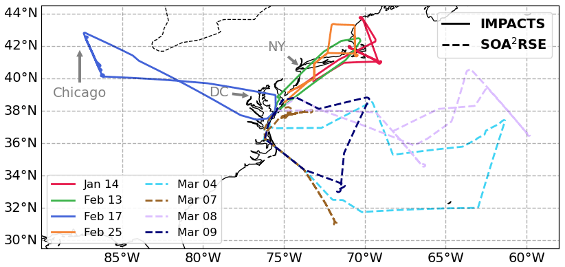
Figure 1 Flight tracks of the P-3 VIPR measurements during the 2022 IMPACTS deployment (solid lines). Flight trajectories were chosen to intersect snowstorm systems. Flight tracks of the P-3 VIPR and HALO measurements during the SOA²RSE deployment (dashed lines), Flight trajectories were aimed towards a range of clear-sky and cloudy conditions over the western Atlantic Ocean. The map displays the east coast of the USA. The border with Canada is shown with a dashed line. Different flight dates are color-coded.

Subsequently, VIPR was modified to use two identical reflectors as separate primary apertures for the transmitting and receiving, in contrast to the previous configuration where a single primary reflector was used. This modification was implemented to facilitate the integration of VIPR into NASA's P-3 aircraft, which utilizes radomes to safeguard the instruments against environmental factors. A picture of VIPR mounted on the bomb bay of the P-3 can be found in Cooper (2022).

More significantly, VIPR also underwent modifications to expand its frequency coverage to approximately 158.6–174.8 GHz, as compared to the previous configuration of 167–174.8 GHz. The broader bandwidth enabled the addition of a third radar frequency further away from the water vapor line center, which was implemented to mitigate retrieval biases associated with frequency-dependent hydrometeor extinction and backscatter (Roy et al., 2021). Table 1 summarizes the major radar system parameters used in this work. Since the Twin Otter airborne measurements, VIPR was reconfigured to operate over a wider bandwidth and to use two separate 38 cm diameter reflector antennas (one for transmit and one for receiver), instead of the previous single 60 cm diameter antenna shared between transmit and receive using a quasioptical duplexing subsystem. The wider tuning bandwidth allows three frequencies to be transmitted instead of two, while the use of separate antennas is compatible with the use of radomes that are necessary for VIPR's flights on higher-flying aircraft. As a consequence of the wider-tuning feature, VIPR's transmit power for the measurements shown here was lower than those made previously.

Table 1 VIPR system parameters.

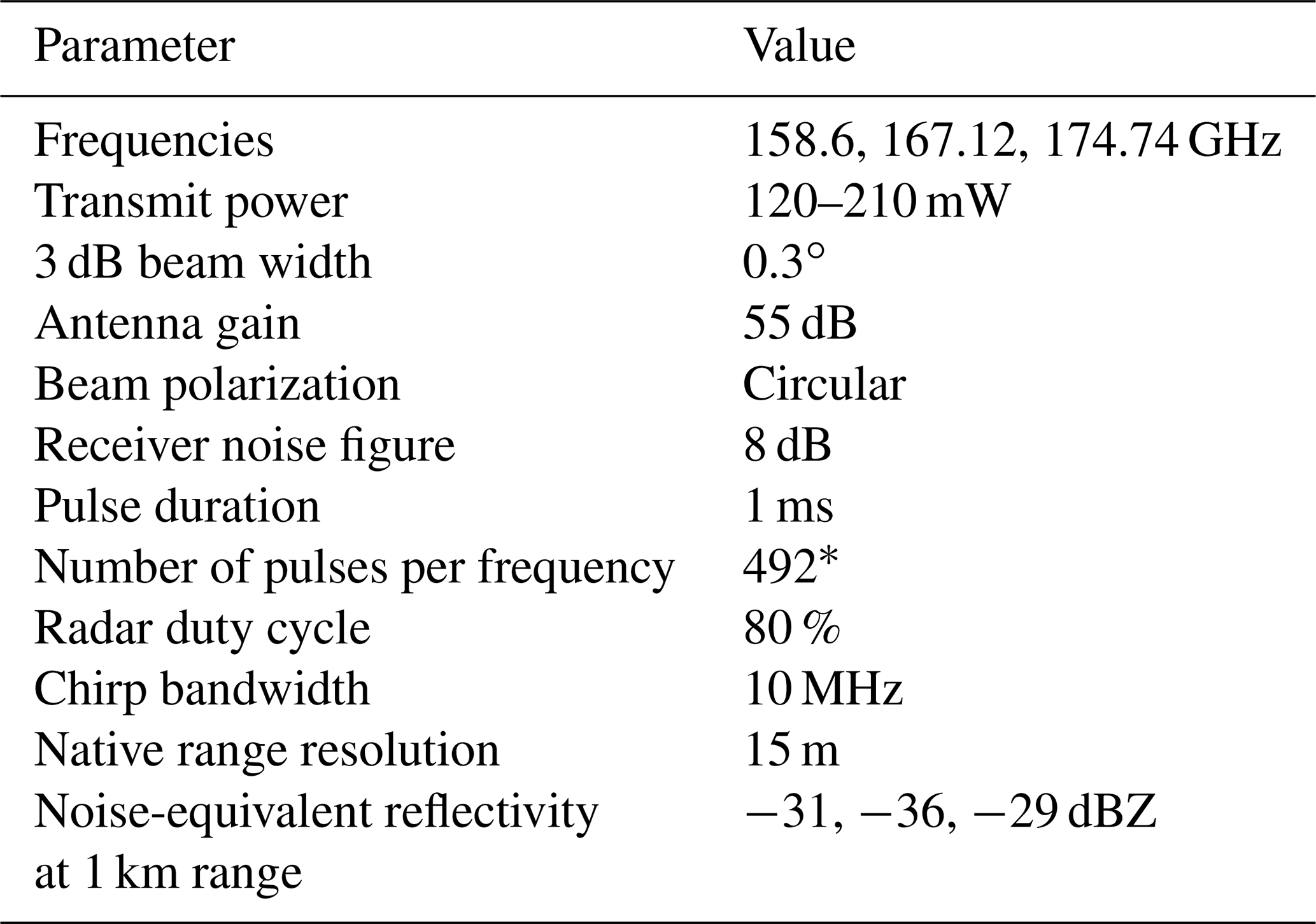
^* 246 chirp-up pulses and 246 chirp-down pulses.

The IMPACTS field campaign, sponsored by NASA, was an Earth Ventures Suborbital (EVS) field campaign aimed at studying high-impact winter snowstorms, particularly cyclones that affect the US east coast (McMurdie et al., 2022). The primary observation platforms for the IMPACTS campaign were the ER-2 and P-3 aircraft. The second deployment of the IMPACTS campaign was conducted from NASA Wallops during January and February 2022. As part of the P-3 payload, VIPR was deployed during four flights, as outlined in Table 2 and depicted in Fig. 1 (solid lines). Most of the VIPR measurements were obtained during flights along the east coast northward of NASA Wallops, with the exception of the 17 February flight, which targeted an in-land snowstorm system.

Table 2 VIPR IMPACTS and SOA²RSE flights details and objectives.

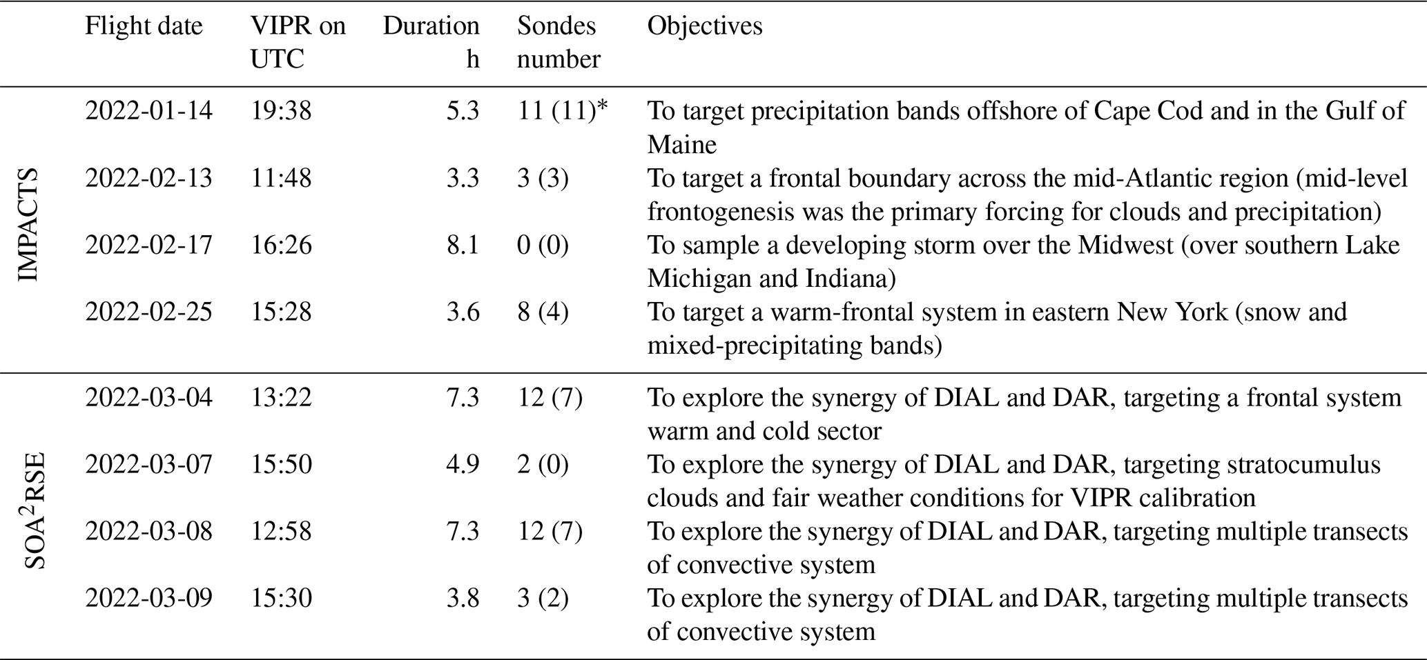
^* The number in brackets indicates the number of sondes under cloudy/precipitating conditions as measured by VIPR.

Following the IMPACTS field campaign, VIPR conducted four additional flights to assess its synergy with the High Altitude Lidar Observatory (HALO) instrument (Carroll et al., 2022) as part of the SOA²RSE campaign, which was sponsored by NASA's Earth Science Technology Office (ESTO). The purpose of SOA²RSE was to demonstrate the synergies of the DIAL and DAR measurement approaches for the first time. These flights were aimed towards a range of clear-sky and cloudy conditions over the western Atlantic Ocean near NASA Wallops Flight Facility. See Table 2 and Fig. 1 (dashed lines) for details. Overall, these flights (IMPACTS and SOA²RSE) encompass around 44 h of VIPR data.

2.1 VIPR measurements and noise subtraction

A full description of the VIPR implementation is provided elsewhere (Cooper et al., 2018, 2021; Roy et al., 2020, 2022). In short, VIPR is a frequency-modulated continuous-wave (FMCW; see Fig. 2) radar measuring reflectivity profiles inside clouds and precipitation at three frequencies (158.6, 167.12, and 174.74 GHz). The fundamental VIPR measurement at each frequency, f, is a power spectrum as shown in Fig. 3. These power spectra are converted to profiles of measured reflected power, P_m(r,f), at each range bin, r, using the standard FMCW signal processing approach (e.g., Cooper et al., 2011). The measured power is the combination of the actual echo power, P_e(r,f), and the noise power, P_n(r,f), that is, $P_{\mathrm{m}}(r,f)=P_{\mathrm{e}}(r,f)+P_{\mathrm{n}}(r,f)$.

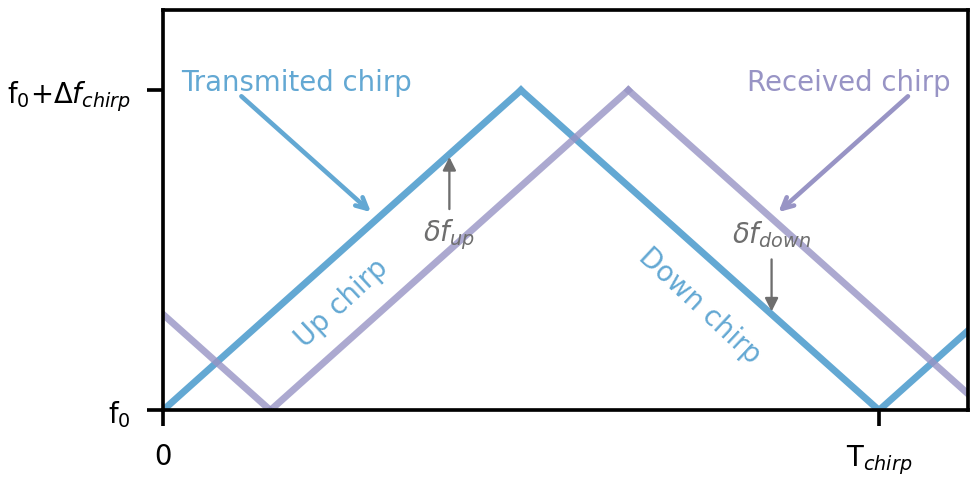
Figure 2 Schematic of FMCW radar ranges. The received chirp is offset in time from the transmit chirp, resulting in an instantaneous frequency difference for a point target of δf, for most of the detection interval, which is proportional to the range of the target according to $\mathit{\delta }f=\mathrm{2}\mathrm{\Delta }{F}_{\text{chirp}}r/c{T}_{\text{chirp}}$, where ΔF_chirp is the chirp bandwidth and T_chirp is the chirp duration. Hence, the IF signal of the receiver mixer in an FMCW radar will have a frequency shift proportional to the range to target. For scenes with hydrometeors at multiple ranges, the IF will contain a linear superposition of frequencies representing the different ranges. Signal processing techniques are then used to convert the IF time-domain signal to a range-resolved power spectrum.

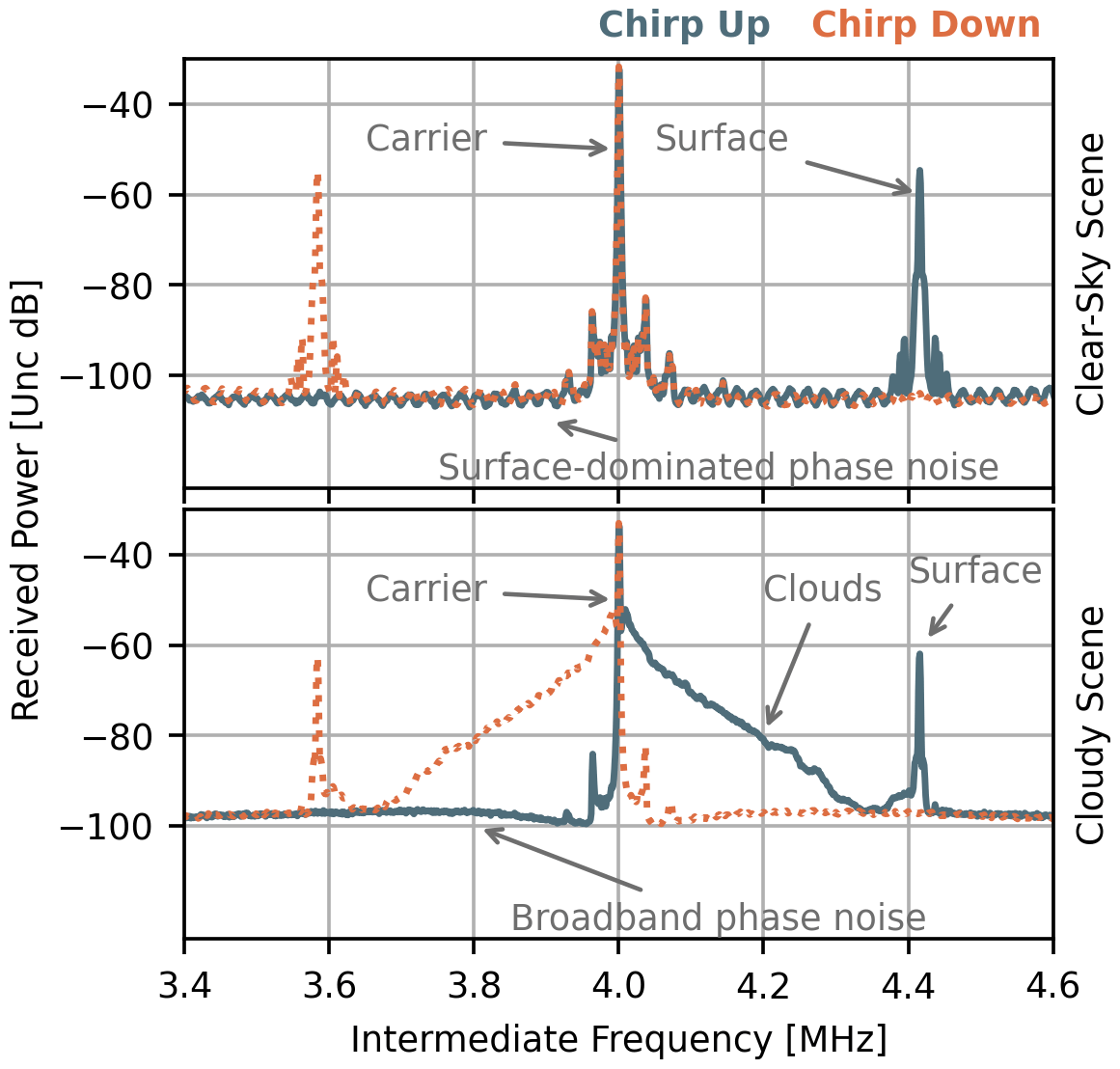
Figure 3 Power spectrum examples at 167.12 GHz for a clear-sky and a cloudy scene. The labels highlight features in the chirp up power spectrum, while mirror features can be found in the chirp down power spectrum. The surface return can be seen around 3.6 or 4.4 MHz depending on the chirp direction. Surface phase noise sidelobes are clearly seen in the clear-sky case. The power spectra at 158.6 and 174.7 GHz are similar, with the former being affected by less water attenuation and the latter by more.

The first step in our data analysis is to estimate P_n(r,f) in each radar range bin so that we can then estimate P_e(r,f) as $P_{\mathrm{e}}(r,f)=P_{\mathrm{m}}(r,f)-P_{\mathrm{n}}(r,f)$. Noise in the VIPR profiles take two forms: (1) thermal noise, which is a characteristic of VIPR's receiver and the scene brightness temperature, and (2) phase noise that is carried by the radar's transmit signal, and hence is more prominent with brighter reflectivity scatterers. The thermal noise can be modeled as P_nT=kT_sysB, where K is Boltzmann's constant, T_sys is the system temperature, and B is the detection bandwidth. Phase noise originates in the radar's local oscillator used to generate the G-band signals, and it causes range side lobes that spread throughout the observed power spectrum.

Through the IMPACTS and SOA²RSE flights, P_n(r,f) is dominated by phase noise, with two distinct forms: a surface-dominated phase noise and broadband phase noise (resulting from multiple echoes originating from clouds and precipitation that are distributed in range). See Cooper (2022) for more details. To illustrate this, Fig. 4a shows a curtain plot of the raw radar reflectivities at 167.12 GHz during a  40 min acquisition over the Atlantic Ocean on 14 January 2022. The surface can clearly be seen around 6 km range as a bright reflection practically at a constant range throughout this curtain. A periodic (in range) clutter signal associated with this reflection is visible above and below the surface. These range side lobes that appear in clear-sky profiles arose from surface-dominant phase noise. As the extent of the clouds and attenuation increases (towards the end of the acquisition), the intensity of the surface reflection and the intensity of this periodic clutter also diminishes. In these profiles, the bright clouds produce their own broadband phase noise that overpowers the phase noise contribution from the surface reflection. That is, the phase noise power from the clouds is broadband, not lobed as for phase noise from a surface reflection, because the clouds extend continuously over a broad range so that there is no dominant lobed-noise contribution from a single range (Cooper, 2022).

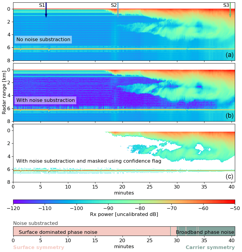
Figure 4 Uncalibrated VIPR 167.12 GHz reflectivities measured during the first ∼40 min of the 14 January flight with no noise subtraction (a), with noise subtraction (b), and with noise subtraction and confidence flag (c). The noise subtraction is indicated by the pink/green bar (for phase noise and thermal noise, respectively).

To illustrate this further, Fig. 5a shows three slices of this curtain. In all three slices the transmit/receive leakage signal can clearly be seen at the aircraft altitude (i.e., at zero range). Additionally the surface return can be seen around 6 km. The first slice (S1, navy line) shows a clear-sky scenario where the clutter induced by the surface return can clearly be seen above and below the surface, that is, the periodic signal with an amplitude of 1 dB and a period of 300 m. The second slice (S2, light blue line) portrays a partly cloudy scene with clouds close the aircraft and at a range of around 2.7 km. The periodic clutter, caused by the surface return, is still visible below and above the surface, but its amplitude has been reduced by the extra attenuation introduced by the clouds. The third slice (S3, green line) shows a cloud extending from the aircraft up to a ∼4.8 km range. In this slice, the additional cloud attenuation has significantly attenuated the surface return leaving no discernable periodic phase noise from the surface reflection, but instead causing a broadband noise increase evident below the surface.

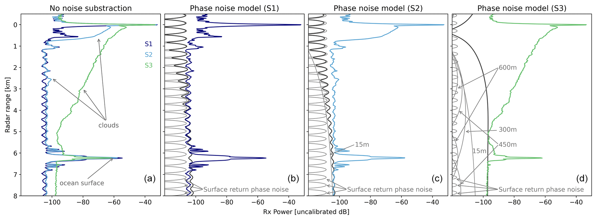
Figure 5 (a) Radar reflectivities at the three slices indicated in Fig. 4, depicting scenarios with clear-sky (S1, navy line, featuring a bright reflection around 6.5 km), a partly cloudy scene (S2, light blue), and a cloudy scene (S3, green). (b–d) Phase noise model simulations for each of these slices. The integrated phase noise model is depicted in dark gray, while phase noise model examples at different ranges are shown in light gray.

Two potential noise subtraction approaches can be applied to the VIPR reflectivities: one associated with the surface-dominant phase noise and the other due to broadband cloud induced phase noise. Both can mask reflections from significantly weaker targets at other ranges. To decide which type of noise subtraction to use, we first model the phase noise associated with the surface following the model described by Cooper (2022). In short, at a given separation in intermediate frequency (IF) between the carrier and the target location, Δf_IF, the point-target phase noise can be simulated as

$$\begin{array}{}\text{(1)}& \mathit{\phi }\left(\mathrm{\Delta }{f}_{\text{IF}}\right)=A+\mathrm{10}{\log }_{\mathrm{10}}\left(F\right)+B\mathrm{\Delta }{f}_{\text{IF}}+C\exp \left({\displaystyle \frac{-\mathrm{\Delta }{f}_{\text{IF}}^{\mathrm{2}}}{D^{\mathrm{2}}}}\right),\end{array}$$

where A is 58 dBc (i.e., decibels relative to carrier), B is −7 dB MHz⁻¹, C is −3 dB, and D is 0.2 MHz. Lastly, F is the interference modulator factor given by

$$\begin{array}{}\text{(2)}& F=\mathrm{4}{\sin }^{\mathrm{2}}\left({\displaystyle \frac{\mathrm{2}\mathit{\pi }R}{c}}\mathrm{\Delta }{f}_{\text{IF}}\right),\end{array}$$

where R is the range to the target location related to the IF following $f_{\text{IF}}=\mathrm{2}KR/c$, where K is the chirp rate in Hz s⁻¹ and c is the speed of light.

Once we have estimated the surface phase noise, we perform a fast Fourier transform (FFT) on the signal below the surface to identify its frequency components. We then analyze the resulting frequency spectrum to see whether a component matches the simulated periodicity of the modeled phase noise surface return (as computed by Eq. 1). If such a match exists we estimate the range-dependent phase noise using the observed sub-surface measured power. We then use the fact that the phase noise is symmetric about the surface to subtract the phase noise from the atmospheric ranges. If the FFT analysis does not match such component, we instead proceed to subtract the broadband phase noise derived from the opposite chirp direction as described by Roy et al. (2018).

Figure 5b–d show examples of this point-target phase noise model (light gray lines). As shown, on Slice 1 (a clear-sky scenario), the modeled phase noise originating from the surface agrees with the observed noise below the surface, providing confidence in the point-target noise model. In Slice 2 (a partly cloudy case) and Slice 3 (a cloudy case), the noise below the surface is well represented by the integration of the point-target models. These point-target curves exhibit a periodicity that is inversely proportional to the range of the carrier tone, along with an amplitude variation in the intermediate frequency. Note how the surface return point-target phase noise model reproduces the behavior discussed in Fig. 4, where the amplitude of its periodic clutter decreases as the surface return gets more attenuated. For instance, in Slice 3 the surface return point-target phase noise model is orders of magnitude smaller than the surface return point-target phase noise model displayed in Slice 1.

Figure 4b shows the same curtain as in the top panel after the noise subtraction. As expected, the contrast between the noise floor and the hydrometeor targets increases improving the dynamic range of VIPR, which improves the detection of weak clouds, such as in Slice 2 around 2.7 km in range. As a reference, Fig. 4 also displays which noise was subtracted throughout the flight.

2.2 Radar detection confidence flag

We create a hydrometeor confidence flag to identify ranges at which the observed reflectivity is associated with an atmospheric target as opposed to noise. This flag is based upon the phase noise model described in the previous section.

The simulated phase noise model as measured by VIPR, φ_M, is given by the sum of the point-target phase noise contributions (Cooper, 2022), that is,

$$\begin{array}{}\text{(3)}& {\mathit{\phi }}_{\mathrm{M}}=\sum _{\text{carrier}}^{\text{surface}}\mathit{\phi }\left(\mathrm{\Delta }{f}_{\text{IF}}\right).\end{array}$$

As shown in Fig. 5b–d (dark gray lines), the summed phase noise agrees with the observed noise below the surface for the three slices. These slices covered different hydrometeor burdens: a clear-sky scenario, a partly cloudy, and a cloudy case for Slices 1, 2, and 3 respectively.

To be considered a radar detection, the returns need to be at least 3 dB greater than the envelope of the integrated phase noise model and to have a signal-to-noise ratio greater than 3. In those cases, the confidence flag is set to one (otherwise it is set to zero). In this context, the detection envelope refers to a curve following the local maxima of the phase noise model to avoid the local minima associated with the periodicity of the surface-reflection phase noise. While we might lose details about thin clouds, these criteria are designed to effectively filter out any spurious returns caused by phase noise rising above the noise floor. See for example the curtains b and c in Fig. 4 by the end of the acquisition (after minute 37, bottom right corner) in the 2 km closest to the surface.

2.3 Calibrated radar reflectivity

After noise subtraction we calculate the calibrated radar reflectivity as

$$\begin{array}{}\text{(4)}& Z_{\mathrm{e}}(r,f)=P_{\mathrm{e}}(r,f)C\left(f\right)r^{\mathrm{2}},\end{array}$$

where C(f) is a calibration factor, and Z_e(r,f) is the reflectivity of a cloudy volume in conventional meteorological units of decibels of mm⁶ m⁻³. VIPR calibration was performed in a ground-based setting using a metallic spherical reflector suspended between two poles by a nylon thread. In simple terms, the calibration factor sets an absolute scale of echo power based on the well-known scattering cross section of the calibration sphere. Details of this procedure can be found in Cooper et al. (2021) and in Roy et al. (2021).

Errors sources in this calibration factor include the following: (1) inaccurate knowledge of the radar's parameters (such as potential drifts in transmit power and receiver noise between the ground calibration and airborne deployment), (2) uncertainties in the water vapor attenuation assumed for the beam path between the instrument and calibration sphere, (3) positioning of the calibration sphere with respect to the beam center, and (4) possible scattering effects of the suspending nylon thread. Based on previous calibration efforts this calibration method suggests an accuracy of 1 to 2 dB (Cooper et al., 2021; Roy et al., 2021), although it may be slightly larger as discussed in Sect. 5.

The calibration we use was performed prior to aircraft installation on 28 September 2021 and also immediately following the removal of VIPR from the P-3 aircraft on 15 March 2022. The re-calibration was done because part way through the campaign, VIPR's low-noise amplifier (LNA) failed and was replaced.

3 Retrieval methodology and datasets used for comparisons

3.1 Water vapor profiling retrieval

The DAR retrieval methodology is fully discussed elsewhere (Roy et al., 2018, 2021, 2022; Battaglia and Kollias, 2019). For completeness, here we provide a recap of a simplified retrieval to provide a heuristic understanding of the minimal DAR physics. The DAR profiling technique begins by combining the observed reflectivities to form the observed absorption coefficient at the two different ranges r₁ and $r_{\mathrm{2}}=r_{\mathrm{1}}+R$:

$$\begin{array}{}\text{(5)}& \mathit{\gamma }(r_{\mathrm{1}},r_{\mathrm{2}},f)={\displaystyle \frac{\mathrm{1}}{\mathrm{2}R}}\ln \left[{\displaystyle \frac{Z_{\mathrm{e}}(r_{\mathrm{1}},f)}{Z_{\mathrm{e}}(r_{\mathrm{2}},f)}}\right],\end{array}$$

where Z_e(r,f) is the measured reflectivity (after noise subtraction) given by

$$\begin{array}{}\text{(6)}& Z_{\mathrm{e}}(r,f)=Z_{\text{eff}}(r,f)e^{-\mathrm{2}\mathit{\tau }(r,f)},\end{array}$$

where Z_eff(r,f) is the effective unattenuated reflectivity for a given target, and τ(r,f) is the one-way optical depth from the radar to the range r.

Thus, Eq. (5) can be rewritten as

$$\begin{array}{}\text{(7)}& {\displaystyle }\mathit{\gamma }(r_{\mathrm{1}},r_{\mathrm{2}},f){\displaystyle }={\displaystyle \frac{\mathrm{1}}{\mathrm{2}R}}\ln \left[{\displaystyle \frac{Z_{\text{eff}}(r_{\mathrm{1}},f)}{Z_{\text{eff}}(r_{\mathrm{2}},f)}}{e}^{-\mathrm{2}\mathit{\beta }(r_{\mathrm{1}},r_{\mathrm{2}},f)R}\right],\end{array}$$

where

$$\begin{array}{}\text{(8)}& {\displaystyle }\mathit{\beta }(r_{\mathrm{1}},r_{\mathrm{2}},f)& {\displaystyle }={\displaystyle \frac{\mathit{\tau }(r_{\mathrm{1}},f)-\mathit{\tau }(r_{\mathrm{2}},f)}{R}}\text{(9)}& {\displaystyle }& {\displaystyle }={\displaystyle \frac{\mathrm{1}}{R}}\underset{r_{\mathrm{1}}}{\overset{r_{\mathrm{2}}}{\int }}\left[\sum {\mathit{\rho }}_j\left(r\right){\mathit{\kappa }}_j(r,f)+{\mathit{\beta }}_{\mathrm{p}}(r,f)\right]\mathrm{d}r\end{array}$$

is the average absorption coefficient between r₁ and r₂, ρ_j(r) is the density of the jth gas, κ_j(r,f) is the corresponding mass extinction cross section (which varies due to pressure and temperature variations along the radar path), and β_p(r,f) is the particulate extinction coefficient. Note that the observed absorption coefficient, $\mathit{\gamma }(r_{\mathrm{1}},r_{\mathrm{2}},f)$, is not affected by absolute calibration. That is, the DAR profiling retrieval is self calibrated. Our calibration procedure described above is instead only relevant to the absolute-dBZ mapping of the clouds and precipitation using VIPR.

This equation can be simplified by separating the water vapor components from the other gases:

$$\begin{array}{}\text{(10)}& \begin{array}{rl}\mathit{\beta }(r_{\mathrm{1}},r_{\mathrm{2}},f)=& \stackrel{\mathrm{‾}}{{\mathit{\rho }}_{\mathrm{v}}}(r_{\mathrm{1}},r_{\mathrm{2}}){\mathit{\kappa }}_{\mathrm{v}}\left(f\right)\\ & +\stackrel{\mathrm{‾}}{{\mathit{\beta }}_{\text{dry}}}(r_{\mathrm{1}},r_{\mathrm{2}},f)+\stackrel{\mathrm{‾}}{{\mathit{\beta }}_{\mathrm{p}}}(r_{\mathrm{1}},r_{\mathrm{2}},f),\end{array}\end{array}$$

where $\stackrel{\mathrm{‾}}{{\mathit{\rho }}_{\mathrm{v}}}$ is the water vapor density, κ_v(f) is the water vapor mass extinction coefficient, and $\stackrel{\mathrm{‾}}{{\mathit{\beta }}_{\text{dry}}}(r_{\mathrm{1}},r_{\mathrm{2}},f)$ is the dry-air absorption coefficient, where the overline indicates taking the average between r₁ and r₂.

Thus Eq. (7) can be rewritten as

$$\begin{array}{}\text{(11)}& {\displaystyle }\mathit{\gamma }(r_{\mathrm{1}},r_{\mathrm{2}},f)=& {\displaystyle }\stackrel{\mathrm{‾}}{{\mathit{\rho }}_{\mathrm{v}}}(r_{\mathrm{1}},r_{\mathrm{2}}){\mathit{\kappa }}_{\mathrm{v}}\left(f\right)+{\displaystyle \frac{\mathrm{1}}{\mathrm{2}R}}\ln \left[{\displaystyle \frac{Z_{\text{eff}}(r_{\mathrm{1}},f)}{Z_{\text{eff}}(r_{\mathrm{2}},f)}}\right]\text{(12)}& {\displaystyle }& {\displaystyle }+\stackrel{\mathrm{‾}}{{\mathit{\beta }}_{\text{dry}}}(r_{\mathrm{1}},r_{\mathrm{2}},f)+\stackrel{\mathrm{‾}}{{\mathit{\beta }}_{\mathrm{p}}}(r_{\mathrm{1}},r_{\mathrm{2}},f),\end{array}$$

which implies that the average humidity between r₁ and r₂ can be extracted by performing a least square fit to this equation, where the last three parameters can be assumed to vary weakly with frequency and contain information about the relative reflectivity of the two ranges in question: the dry air gaseous absorption and the particulate extinction respectively. In principle, all three have a weak frequency dependence.

As shown by Roy et al. (2018), when using two radar tones at different frequencies, the humidity can be estimated directly using

$$\begin{array}{}\text{(13)}& \stackrel{\mathrm{‾}}{{\mathit{\rho }}_{\mathrm{v}}}(r_{\mathrm{1}},r_{\mathrm{2}})={\displaystyle \frac{\mathit{\gamma }(r_{\mathrm{1}},r_{\mathrm{2}},f_{\mathrm{2}})-\mathit{\gamma }(r_{\mathrm{1}},r_{\mathrm{2}},f_{\mathrm{1}})}{{\mathit{\kappa }}_{\mathrm{v}}\left(f_{\mathrm{2}}\right)-{\mathit{\kappa }}_{\mathrm{v}}\left(f_{\mathrm{1}}\right)}},\end{array}$$

which assumes that the last three terms in Eq. (7) are a frequency-independent offset. However, this may not be necessarily true in regions where the particle size distributions of hydrometeors vary significantly in range, such as near cloud boundaries or in regions with phase changes. In those situations, the range-dependent differential scattering of hydrometers can be erroneously attributed to water vapor, resulting in measurement bias. If more than two frequencies are used, the retrieval can partly disentangle the differential extinction from the water vapor from the hydrometeor scattering and absorption effects as shown by Battaglia and Kollias (2019) and Roy et al. (2022).

The uncertainty in $\mathit{\gamma }(r_{\mathrm{1}},r_{\mathrm{2}},f)$ can be computed using standard error propagation techniques (Roy et al., 2018; Battaglia and Kollias, 2019). This uncertainty can then be used to estimate the humidity uncertainty. In this study, from the 15 m native VIPR reflectivity resolution, we use steps of 300 m (i.e., R=300 m) to derive the in-cloud profiles, which have an associated precision of around 5.5 g m⁻³. This results in a water vapor profile with 300 m vertical resolution sampled every 15 m. These oversampled estimates are then averaged to a 300 m vertical grid to smooth out the retrievals, improving the precision by a factor of $\sqrt{\mathrm{20}}$ (i.e., to around 1.23 g m⁻³). These types of water profiles are taken every 1.9 s, which is the time that it takes VIPR to cycle through the three frequencies for the programmed number of pulses per frequency. This temporal resolution results in an approximate along-track resolution of 320 m assuming a 607 km h⁻¹ average P-3 speed.

3.2 Partial column water vapor retrieval

As shown by Roy et al. (2022), when using two radar tones at different frequencies, the partial column water vapor (pCWV) can be estimated using

$$\begin{array}{}\text{(14)}& {\displaystyle }\text{pCWV}={\displaystyle \frac{\cos \left({\mathit{\theta }}_i\right)}{\mathrm{2}\langle \mathrm{\Delta }{k}_{\mathrm{v}}\rangle }}{\displaystyle \frac{{\mathit{\sigma }}_{\mathrm{m}}^{\mathrm{0}}\left(f_{\mathrm{1}}\right)}{{\mathit{\sigma }}_{\mathrm{m}}^{\mathrm{0}}\left(f_{\mathrm{2}}\right)}},\end{array}$$

where θ_i is the beam pointing angle relative to the local nadir, ${\mathit{\sigma }}_{\mathrm{m}}^{\mathrm{0}}\left(f\right)$ is the measured surface normalized radar cross section at a given frequency, and

$$\begin{array}{}\text{(15)}& {\displaystyle }\langle \mathrm{\Delta }{k}_{\mathrm{v}}\rangle ={\displaystyle \frac{{\int }_{\mathrm{0}}^{R_s}{\mathit{\rho }}_{\mathrm{v}}\left(r^{\prime }\right)\mathrm{\Delta }{k}_{\mathrm{v}}\left(r^{\prime }\right)\mathrm{d}{r}^{\prime }}{{\int }_{\mathrm{0}}^{R_s}{\mathit{\rho }}_{\mathrm{v}}\left(r^{\prime }\right)\mathrm{d}{r}^{\prime }}},\end{array}$$

where $\mathrm{\Delta }{k}_{\mathrm{v}}\left(r\right)=k_{\mathrm{v}}(f_{\mathrm{2}},T(r),p(r\left)\right)-k_{\mathrm{v}}(f_{\mathrm{1}},T(r),p(r\left)\right)$ is the local differential absorption cross section for water vapor per unit mass, which changes with temperature, T(r), and pressure, p(r), along the radar path. Thus by assuming a given temperature and pressure profile, and the shape of a water vapor profile, pCWV can be inferred. That is, the normalization of Eq. (15) ensures that the pCWV retrieval only depends on the humidity profile shape assumed.

As with the profile retrieval, when using only two frequencies the inferred pCWV may be subject to biases induced by frequency-dependent attenuation contributions from the cloud and precipitation hydrometeors along the radar path. If more than two frequencies are used, the retrieval can distinguish the differential extinction from the water vapor from the hydrometeor absorption effects as shown by Roy et al. (2020).

Note that for these retrievals accurate relative calibration factors are needed. The pCWV precision at the native VIPR resolution is ∼5 kg m⁻², which corresponds to the time that it takes VIPR to cycle trough the three frequencies, that is, 1.9 s (approximately 320 m).

3.3 Ancillary retrieval information

Both the profiling and the pCWV retrievals require ancillary pressure and temperature information. This information is obtained from the Modern-Era Retrospective Analysis for Research and Applications version 2 (MERRA-2) reanalysis (Gelaro et al., 2017), which provides fields every 3 h on a 0.625 by 0.5^∘ longitude–latitude grid with a vertical resolution better than 1 km in the lower troposphere. In the retrievals, we simply find the closest grid point to the VIPR measurement in the 12:00 UTC MERRA-2 fields. Note that, as shown by Roy et al. (2018), the retrieved humidity is weakly dependent on the assumed pressure and only accrues a 10 % error for an 8 K temperature deviation. For the pCWV retrievals the retrieval also assumes the normalized shape of the humidity profile (Roy et al., 2022), which is also derived from MERRA-2. This profile shape is needed to quantify the absorption line broadening, which depends on temperature and pressure. The assumed water vapor profile shape is then scaled by a multiplicative factor to match the observed ratios of the radar surface reflectivity. While we use MERRA-2 for ancillary information, we later use ERA5 as an independent reanalysis dataset against which the retrievals are compared as detailed in Sect. 3.5.

All retrievals shown here only use radar returns classified as confident using the flag described in Sect. 2.2. In this article we only show results from the chirp-up estimates. We acknowledge that the chirp-down estimates are nearly identical but display some signs of distortion, the cause of which is under investigation. If we were to average both chirp-up and chirp-down measurements, the improvement in estimate precision would be a factor of $\sqrt{\mathrm{2}}$. However, considering the magnitude of the possible systematic biases and differences between the datasets discussed in Sect. 4, such averaging is deemed unnecessary.

3.4 Dropsondes

Dropsondes were deployed from the P-3 using the Advanced Vertical Atmospheric Profiling System (AVAPS) operated by NASA Langley Research Center (Hock and Franklin, 1999). The AVAPS Global positioning System (GPS) dropsondes measure pressure, temperature, humidity, wind speed, and wind direction as the parachuted dropsonde descends towards the surface. The AVAPS system has been used in many field campaigns (e.g. Wang et al., 2015; Sorooshian et al., 2019; McMurdie et al., 2022; Reid et al., 2023). The dropsondes used in the flights used in this study were the NCAR Research Dropsonde NRD41 manufactured at NCAR. Typical uncertainties are ±0.5 hPa, 0.2 ^∘C, 3 %, and 0.5 m s⁻¹ for pressure, temperature, humidity, and wind respectively.

The NRD41 and RD41 dropsonde family uses a heated humidity sensor, which has minimal biases measuring water vapor inside clouds and thus is well suited for comparisons of humidity measurements in cloudy environments. In addition, the direction of the profile during descent contains no significant risk for icing of the sensors. Prior to take-off of each research flight, the humidity sensors of all dropsondes were properly reconditioned to minimize any calibration drifts that may have happened between production and use of the dropsondes. No correction needed to be applied for the time response of the dropsonde humidity sensors during IMPACTS and SOA²RSE, because the temperature range for these observations was sufficiently warm and the humidity sensor sufficiently fast.

The dropsondes were processed through the Atmospheric Sounding Processing ENvironment (ASPEN,  Martin and Suhr, 2023), to apply all required quality control and correction algorithms. Dropsonde data collected during IMPACTS and SOA²RSE were not transmitted to the WMO Global Telecommunication System and were not assimilated in models. Therefore, the reanalysis comparisons shown in the subsequent sections are not influenced by the dropsonde data and represent a truly independent analysis of the atmosphere in this region.

3.5 ERA5 reanalysis fields

We use data from the European Center for Medium-range Weather Forecasts (ECMWF) global reanalysis fifth generation (ERA5) hourly fields (Hersbach et al., 2023) for intercomparison with the VIPR retrievals. ERA5 combines a high-resolution atmosphere modeling system with observations via a 4-D variational data assimilation. Extensive conventional and satellite observations of humidity are assimilated such as radiosondes as well as radiances from the Microwave Humidity Sounder and the Microwave Humidity Sounder 2 instruments on board NOAA-18, NOAA-19, and FY-3C, along with radiances from the Meteorological Operational (MetOp) satellites. ERA5 provides an hourly record of the ocean, land, and atmospheric state with a ∼31 km horizontal resolution and 137 levels covering from the surface to 0.01 hPa (Hersbach et al., 2020). To ease comparison, we identified the nearest ERA5 humidity field spatially and temporally.

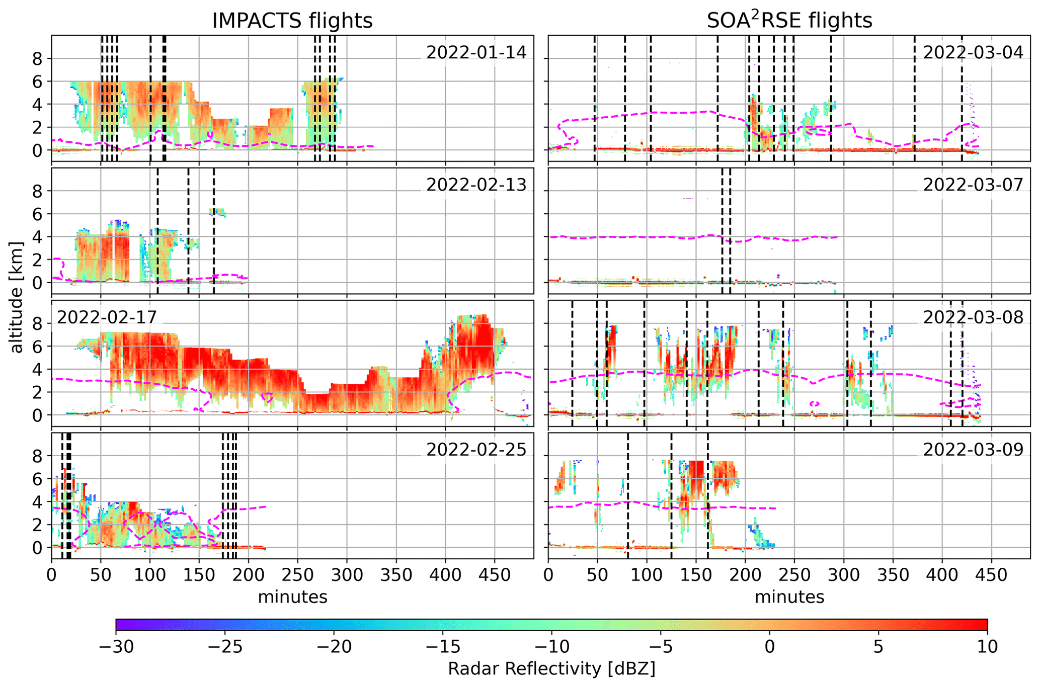
Figure 6 Calibrated radar reflectivities at 167.12 GHz for the IMPACTS (left) and the SOA²RSE (right) flights. Dropsondes launches are indicated by dashed vertical lines. Dashed magenta lines depict the melting layer derived by interpolating the ERA5 reanalysis fields to the VIPR measurement times and locations.

To the best of our knowledge, limited comparisons have been made between ERA5 humidity fields and other datasets. A study by Gamage et al. (2020) compared ERA5 with unassimilated sondes launched from Payerne, Switzerland. That comparison suggests that below ∼1.5 km ERA5 relative humidity is too dry (up to 20 % RH), while between 1.5–5 km ERA5 is 8 % RH wetter. Comparisons with COSMIC-2 water vapor suggest that these datasets agree overall within 6 %–12 %, with larger difference in regions with frequent convection (Johnston et al., 2021). Thus, our study serves as an additional validation albeit limited for ERA5 lower tropospheric humidity fields.

4 Vapor profile results

Figure 6 shows the curtain plots of the radar reflectivities at 167.12 GHz through the IMPACTS and SOA²RSE flights (after applying the confidence flag and subtracting the appropriate noise). The effects of attenuation by a combination of liquid hydrometeors and water vapor are clearly seen in these reflectivities. For example, noticeable attenuation is observed throughout much of the flight on 14 January below 2 km due to precipitation. Similar attenuation is observed below regions with a heavy hydrometeor burden, as seen during the 17 February flight, especially around 420 min into the flight.

Figure 7 shows the curtain plots of the VIPR water vapor estimates for the IMPACTS flights and Fig. 8 for the SOA²RSE flights. To reduce noise, these curtains show 1 min averages of the VIPR retrievals, that is, up to 30 profiles that are taken every ∼2 s. Assuming a flight speed of 607 km h⁻¹, this corresponds to an along-track averaging distance of ∼10 km. Note that the average is performed on the water vapor retrieval instead of the radar reflectivities because the mapping of radar reflectivity ratios into water vapor is non-linear. For intercomparison and to help with the interpretation, these figures also show the curtain plots of the ERA5 water vapor estimates.

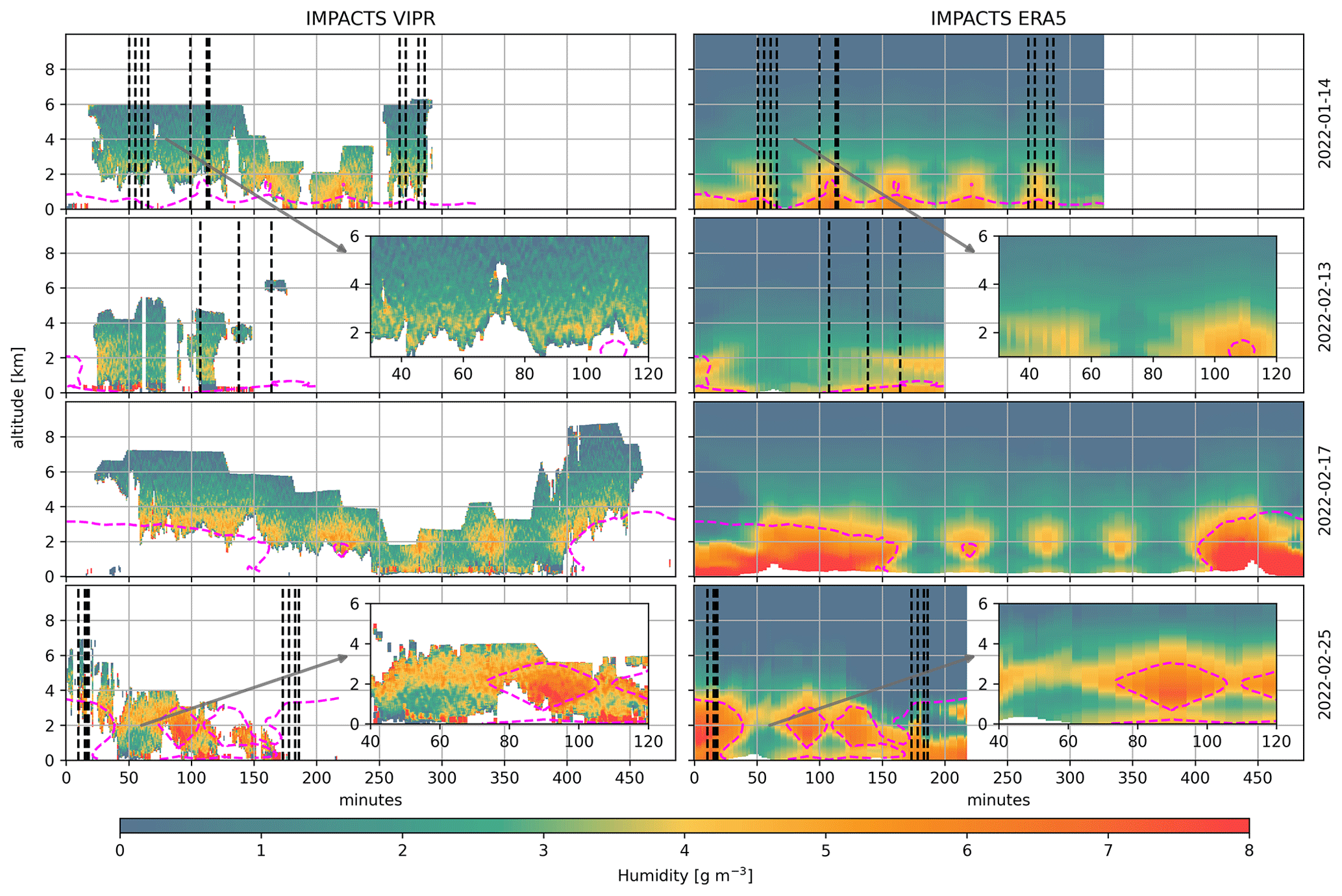
Figure 7 VIPR humidity measurements and ERA5 reanalysis fields for the IMPACTS flights shown in Fig. 6 left. Dropsondes launches are indicated by dashed vertical lines. Dashed magenta lines depict the melting layer. The insets showcase VIPR's ability to capture high-resolution humidity variations within the snowstorms. For these insets the raw VIPR data were smoothed using a 300 m running average in the vertical, as well as a 1 min running average in the horizontal.

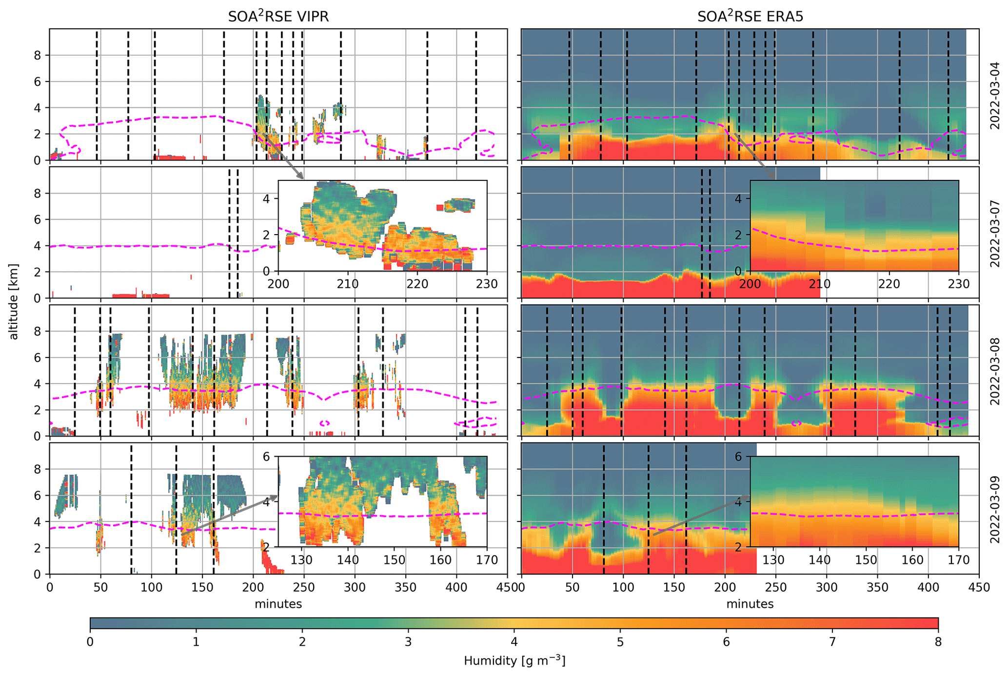
Figure 8 VIPR humidity measurements and ERA5 reanalysis fields for the SOA²RSE flights shown in Fig. 6 right. Dropsondes launches are indicated by dashed vertical lines. Dashed magenta lines depict the melting layer. The insets showcase VIPR's ability to capture high-resolution humidity variations within the clouds. For these insets the raw VIPR data were smoothed using a 300 m running average in the vertical, as well as a 1 min running average in the horizontal.

Overall, VIPR and ERA5 are in good qualitative agreement. Both datasets depict moisture bands (i.e., high moisture regions) associated with snow bands on the 14 January, 17 February, and 25 February flights; a dry layer (moisture <3 g m⁻³) between 40 and 100 min into the 13 February flight; and a strong humidity gradient at around 3–4 km throughout much of the 8 and 9 March flights. Figures 7 and 8 insets demonstrate VIPR's ability to capture high-resolution humidity variations within clouds and precipitation. While some of these variations may be due systematic biases, the presence of structured variability strongly suggests real water vapor variations.

To round up the VIPR/ERA5 intercomparison, Fig. 9 presents percentage differences between VIPR measurements and ERA5 reanalysis fields. During IMPACTS, VIPR and ERA5 agree within 20 % except in the moisture bands on the 17 February flight, where ERA5 seems underestimate the VIPR estimates by up to 50 %, as well as at the cloud/snowstorm edges (top and bottom) where VIPR retrieval artifacts could be the culprits of such differences. During SOA²RSE, ERA5 displays up to a 50 % underestimation of the VIPR estimates above ∼4 km. This underestimation is corroborated by the dropsonde comparison as discussed below.

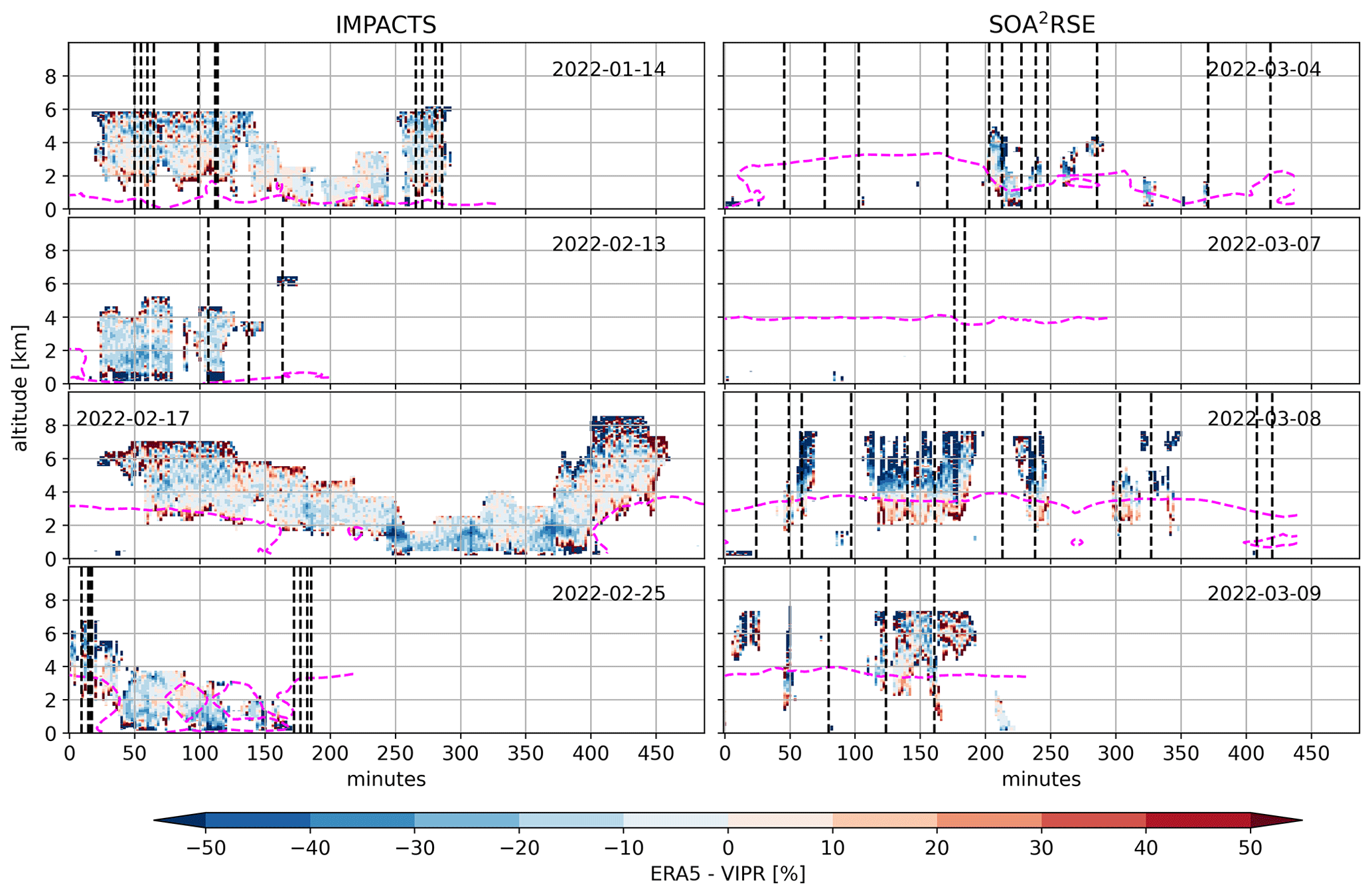
Figure 9 Percentage differences between the ERA5 and VIPR humidity estimates for the IMPACTS (right) and the SOA²RSE (left) flights. Dropsondes launches are indicated by dashed vertical lines. Dashed magenta lines depict the melting layer.

Figure 10 shows a comparison with dropsondes for both VIPR measurements and ERA5 reanalysis fields to further explore their validity. Dropsondes were selected to demonstrate varying retrieval performances, particularly highlighting biases between the two and three frequency retrievals (see below). We included at least one dropsonde from each flight with cloudy measurements. VIPR measurements and ERA5 reanalysis fields are averaged for 10 min around the dropsonde release time, that is, 5 min before and 5 min after (allowing averaging up to 300 profiles, that is, approximately 100 km along track). This averaging, if random measurement errors are dominant over systematic errors (which is not generally the case), would in principle result in a water vapor retrieval precision as good as ∼0.07 g m⁻³ ($\mathrm{1.23}/\sqrt{\mathrm{300}}$). The 10 min average was chosen to reduce noise, especially when comparing it against the radiosondes dropped during SOA²RSE, where the clouds were scattered, in contrast to the continuous cloud cover during IMPACTS.

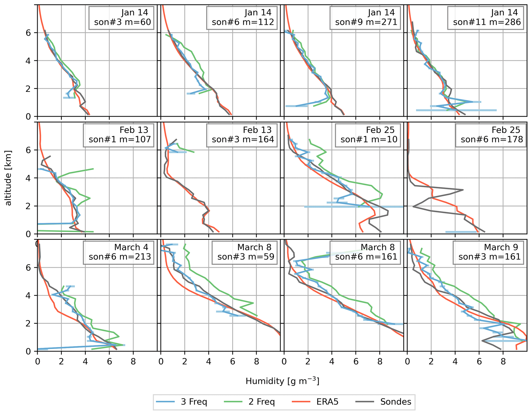
Figure 10 Profile comparisons between dropsondes, VIPR measurements, and ERA5 reanalysis fields. VIPR and ERA5 measurements were averaged over 10 min around the dropsonde time. Two VIPR estimates are shown: one using three radar tones to alleviate hydrometeor influence and one using only two radar tones (167.12 and 174.74 GHz). Error bars (i.e., the averaged random uncertainties) are shown for the three radar tone retrievals, but they are barely visible due to the temporal averaging. Note that ERA5 and the dropsonde humidities were interpolated to the VIPR vertical grid. The legends display the flight date, sonde number, and the minutes into the flight when the sonde was dropped.

Two VIPR estimates are shown: one using three radar tones that should alleviate the hydrometeor influence (Roy et al., 2021) and one using only two radar tones (167.12 and 174.74 GHz). The influence of hydrometeors is clearly discernible in the two-tone estimates (green lines in Fig. 10) for 14 January sondes 3 and 6, 13 and 25 February sonde 1, and all comparisons in March. In these cases, there is an overall high bias which can be attributed to frequency-dependent attenuation caused by hydrometeors being incorrectly attributed to water vapor. Note that the three-tone estimates (blue lines) effectively mitigate these biases and agree much better with the dropsondes through all comparisons shown in Fig. 10. These results clearly indicate that the DAR retrievals should be considered most accurate when using the three-frequency approach outlined in Roy et al. (2021) and demonstrated with data for the first time here.

Another distinct problem with both retrievals (using two or three radar tones) is a scattering effect most evident near cloud boundaries which can result in significant errors of either sign. This is particularly evident in the 13 February sonde 1 and the 4 March sonde 6. In these cases, even though we average over 10 min around the dropsonde, there were not enough valid retrievals to offset the artifacts.

Figure 11 displays scatterplots between VIPR, ERA5, and dropsondes color-coded by height. Note that we only compare the altitudes at which they were at least 150 VIPR water vapor estimates (less than half of the maximum number for the 10 min window). The ERA5 comparisons are separated into cloudy and clear-sky regions as determined by VIPR. Thus, the cloudy comparisons allow a direct intercomparison of ERA5 and VIPR against dropsondes. IMPACTS and SOA²RSE flights are compared separately since they flew over completely different cloud regimes.

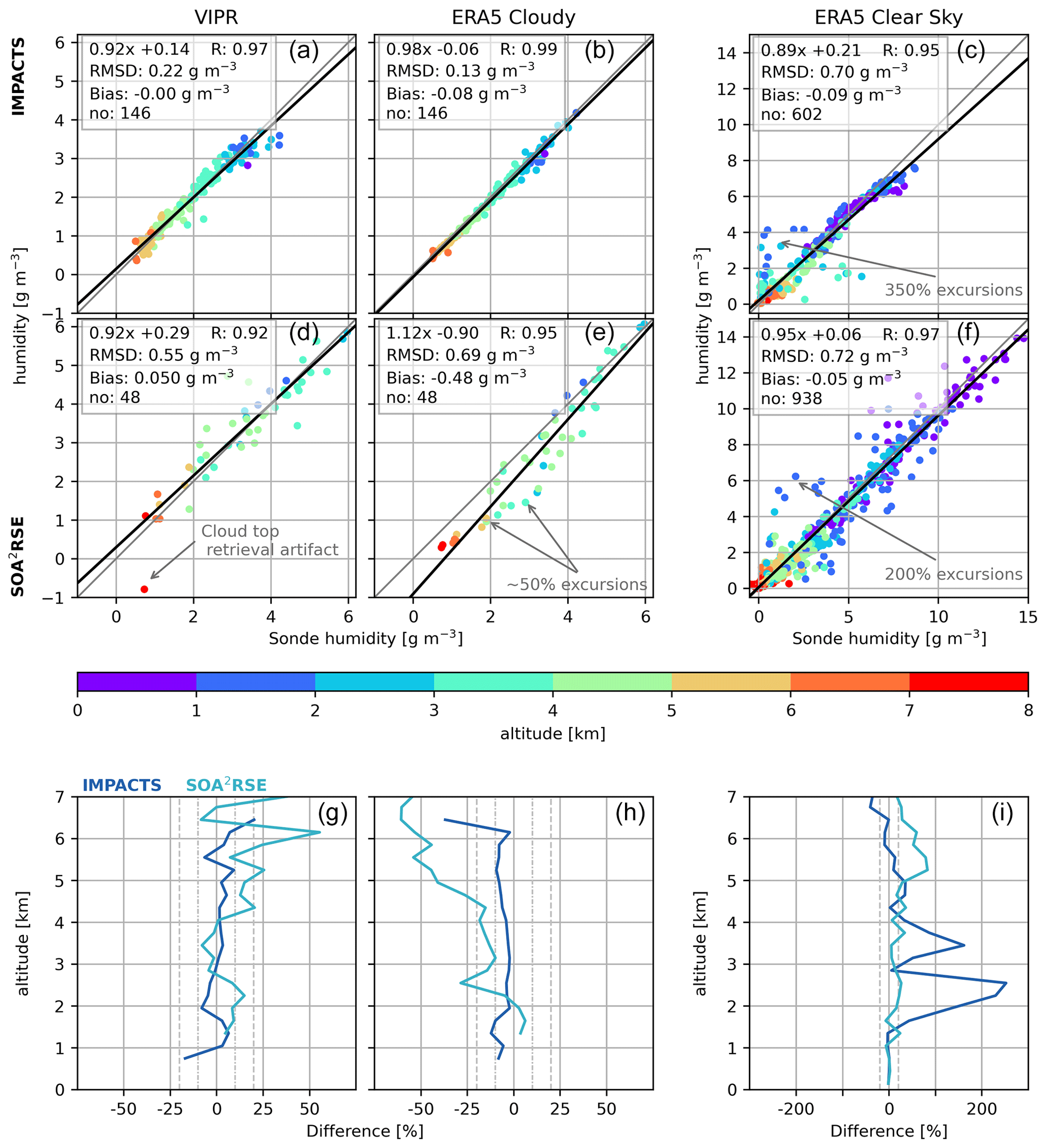
Figure 11 (a–f) Dropsonde humidity measurements scattered against VIPR and ERA5 estimates. The ERA5 comparisons are separated between cloudy and clear-sky regions as measured by VIPR. (g–i) Average biases between VIPR, ERA5, and the dropsondes launched during the IMPACTS (dark blue) and the SOA²RSE flights (light blue). The dashed vertical gray lines indicate the ±20 % difference, while the dashed–dotted vertical gray lines indicate the ±10 % difference. Note that VIPR and ERA5 humidities were averaged over 10 min around the dropsonde launch (approximately 100 km along track). All the available dropsondes were used on these comparisons: 22 and 29 dropsondes during IMPACTS and SOA²RSE respectively.

The VIPR comparisons (for either the IMPACTS or SOA²RSE flights) when averaged over 10 min suggest a reasonably good agreement with the dropsondes (with a root mean square deviation, RMSD, better than 0.55 g m⁻³, and an overall bias better than 0.05 g m⁻³). Similarly, ERA5 agrees extremely well against the dropsondes during the IMPACTS-cloudy scenarios (RMSD=0.13 g m⁻³ and $\text{bias}=-\mathrm{0.08}$ g m⁻³). However, the ERA5 does not agree nearly as well with the sondes during the SOA²RSE-cloudy scenes (RMSD=0.69 g m⁻³ and $\text{bias}=-\mathrm{0.48}$ g m⁻³), with ERA5 displaying clear underestimations for values above 4 km. We speculate that the decreased fidelity of the ERA5 estimates in the SOA²RSE campaign (in contrast with the IMPACTS ones) results from the fact that these flights took place in more subtropical latitudes characterized by isolated convection that is less well constrained by synoptic-scale dynamics in the data assimilation system than the large-scale mid-latitude snowstorms targeted during the IMPACTS flights. Specifically we speculate that the model's convective parameterization may not be producing enough convective transport of moisture out of the planetary boundary layer into the lower free troposphere during these flights.

To explore this further, Fig. 11g–i summarize the biases versus altitude between VIPR, ERA5, and the dropsondes. During IMPACTS, VIPR water vapor estimates agree within 10 % with the dropsondes through most heights. ERA5 also agrees within 10 % (or better) during the cloudy scenes. During SOA²RSE, VIPR water vapor estimates agree within 20 % with the dropsondes through most heights. However, there are some spikes around 6 and 7 km that can be mitigated by either using the median instead of the mean or by removing water vapor estimates that are more than 3 standard deviations from the mean when averaging over the 10 min period used in these comparisons. ERA5 agrees within 20 % with the dropsondes below 4 km. However, above ∼4 km ERA5 displays an underestimation of up to 50 % in cloudy conditions, thus corroborating the VIPR comparison shown in Fig. 9.

Under clear-sky scenarios, ERA5 shows overall good agreement against the dropsondes (with RMSD better than 0.72 g m⁻³, and an overall bias better than −0.05 g m⁻³) but displays large excursions from the one-to-one line, as large as 350 % in some instances. During IMPACTS, these excursions translate to biases of up to 250 % around 2.5 km and up to ∼100 % around 3.5 km.

Overall, the cloudy and clear-sky comparisons indicate good agreement between ERA5 and the dropsondes at the core of the snowstorms but not at the edges. That is, ERA5 is presumably failing to simulate the extent of the snowstorms likely due to its temporal and horizontal resolution that, even though they are the finest among the current reanalyses, they are still too coarse to resolve the rapidly changing snowstorm's extent. During SOA²RSE, ERA5 agrees within 20 % with the dropsondes below 5 km but shows an overestimation of up to 80 % at higher altitudes.

5 Partial column results

Figure 12 shows the scatter between VIPR and dropsondes pCWV estimates for two sets of VIPR reflectivities: one using the sphere calibration factors described in Sect. 2.3 and the other employing a modified set of calibration factors (discussed below). For this comparison, the VIPR measurements were temporally averaged by 10 min, 5 min before and after the dropsonde launch. This amounts to averaging around 300 individual estimates, equivalent to ∼100 km (assuming an average P-3 speed of 607 km h⁻¹), with a theoretical error of around 0.3 kg m⁻² (i.e., $\mathrm{5}/\sqrt{\mathrm{300}}$). These comparisons encompass clear-sky and cloudy scenes demonstrating the all-sky capability of DAR.

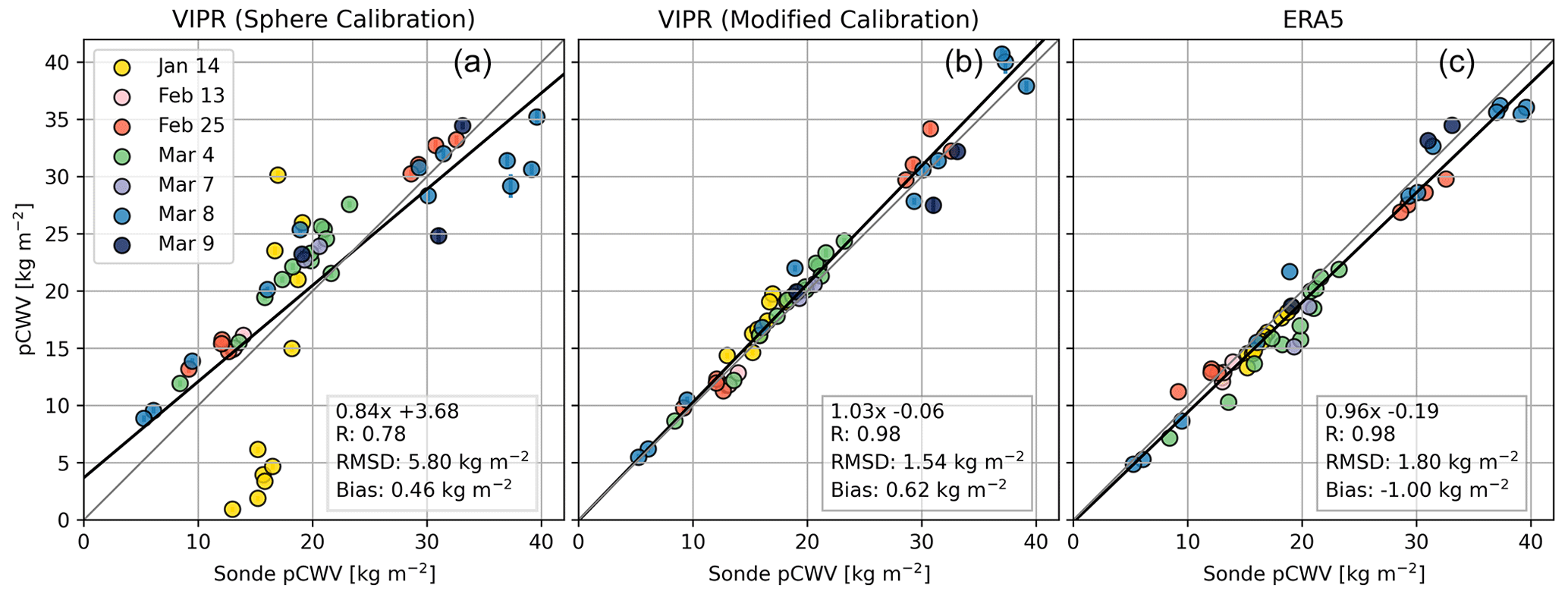
Figure 12 Dropsonde pCWV measurements scattered against the VIPR pCWV estimates using the sphere calibration (a), a modified calibration (b), as well as against the ERA5 pCWV (c). The gray line is the one-to-one line. The solid black line displays a linear fit. The root mean square deviation, the linear fit equation, and the bias are shown for each comparison. Measurements from different days are shown in different colors. The VIPR errors are around 0.3 kg m⁻² (i.e., $\mathrm{5}/\sqrt{\mathrm{300}}$), which are smaller than the symbol size. There are 51 points on these comparisons, one per each available dropsonde (22 during IMPACTS and 29 during SOA²RSE).

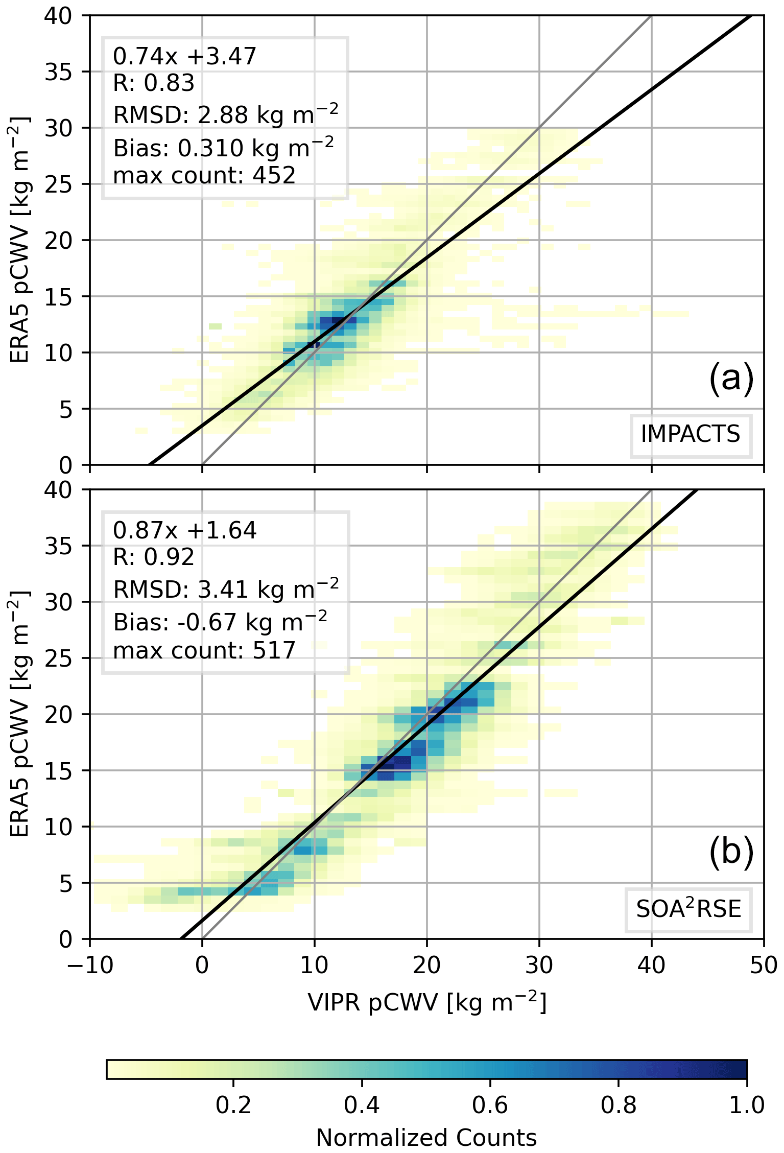
Figure 13 Two-dimensional normalized histograms derived from VIPR and ERA5 pCWV during IMPACTS (a) and SOA²RSE flights (b). These histograms were computed at the native VIPR resolution (i.e., no averaging). The gray line is the one-to-one line. The solid black line displays a linear fit. The root mean square deviation, the linear fit equation, the bias, and the maximum number of counts are shown for each comparison.

A key difference between profiling with DAR and measuring the pCWV is that pCWV requires accurate relative calibration of the radar frequencies. Figure 12a shows the scatter between the dropsondes and the VIPR pCWV estimates that use the sphere calibration factors as described in Sect. 2.3. The best-fit line has a slope of 0.84, an RMSD of 5.8 kg m⁻², and a correlation coefficient (R) of 0.78 with a bias of 0.46 kg m⁻². Although these results suggest a reasonable agreement between the two datasets, they are biased by the estimates from the 14 January flight (yellow dots), which are the only estimates in Fig. 12 using the calibration factor estimated on 28 September 2021 prior to the LNA failure. By simply changing the sphere calibration factor of the 167.12 GHz tone from 8.9 to 12.9, the agreement against the dropsondes (see Fig. 12b) improved considerably. Similarly, by adjusting the sphere calibration factor (post LNA failure) of the 158.6 GHz tone from 10.7 to 12.2, the estimates for the rest of the flights aligned much better with the one-to-one line.

The modifications to the sphere calibration factors were found by trial and error. We emphasize that this recalibration procedure only ensures that the frequencies are calibrated among each other and should not be considered absolute calibrations. Absolute calibration is not required for any DAR water vapor estimation but would be important in any effort to derive cloud microphysical properties. We are continuing work to investigate sources of ground-calibration uncertainty and improve its reliability.

After applying the modified calibration factors (Fig. 12b), there is a noticeable improvement in the comparison metrics. The best-fit line slope increases to 1.03, and the RMSD decreases to 1.54 kg m⁻². The correlation coefficient improves to 0.98, while the bias becomes 0.62 kg m⁻².

Note that the RMSD is much larger than the analytical VIPR uncertainty, 0.3 kg m⁻², presumably due to a combination of factors: (1) the sondes can be quickly advected away from the drop location (with horizontal displacements of up to ∼22 km at the surface), which may introduce collocation errors. (2) During the 10 min window, used for this comparison, even the dropsondes disagree among each other due to the quickly changing nature of the snowstorms scenes. For example, the second, third, and fourth dropsondes during the 14 January flight were dropped in a 10 min span and have an RMSD (with respect to their mean value) of 1.5 kg m⁻². Similarly, the first four dropsondes and the last four dropsondes of the 25 January flight were dropped in a 8 and 13 min span, respectively, and have RMSDs of 1.5 and 1.3 kg m⁻², which may explain the RMSD values shown in the VIPR–sonde comparison (Fig. 12b).

Figure 12c shows the scatter versus the ERA5 pCWV estimates. These estimates are derived from the nearest fields to the VIPR times and locations. That is, for each VIPR measurement, we identified the nearest field, and then we averaged them in the same fashion as the VIPR pCWV estimates to allow for a direct comparison. ERA5 shows an excellent agreement with the sonde measurements, with a best-fit line slope of 0.96, an RMSD of 1.8 kg m⁻², a correlation coefficient of 0.98, and a bias of 1.0 kg m⁻².

To conclude the pCWV comparison, Fig. 13 displays joint histograms of VIPR and ERA5 pCWV estimates (at the VIPR native temporal resolution, i.e., 1.9 s). The regression analyses suggest either an underestimation by the ERA5 reanalysis or an overestimation by the VIPR measurements for both IMPACTS and SOA²RSE flights. Given that the VIPR measurements are not expected to differ significantly from the measurements obtained around the dropsonde sites (as seen in Fig. 12b), we hypothesize that the slight disagreement is likely due to an ERA5 underestimation. We note that the VIPR precision error, which is approximately 5 kg m⁻² at this resolution, accounts for most of the RMSD. Further, other VIPR systematic effects maybe at play, such as drift in its sensitivity or non-ideal surface scattering (e.g., non-random speckle averaging).

6 DAR and DIAL synergy

During the SOA²RSE flights the High Altitude Lidar Observatory (HALO) water vapor DIAL (Carroll et al., 2022) flew in conjunction with VIPR on the same P-3 aircraft to study the synergy of the DIAL and DAR techniques. HALO uses four wavelengths spread among different strength absorption features in the 935 nm water vapor line complex to provide water vapor sensitivity across the vastly different regimes in the troposphere and lower stratosphere. HALO also uses the high spectral resolution and backscatter measurements at 532 and 1064 nm, respectively, for cloud and aerosol profiling (Hair et al., 2008; Carroll et al., 2022). The HALO water vapor retrievals presented here have a resolution of $\mathrm{300}\mathrm{m}\times \sim \mathrm{6}\mathrm{km}$ vertical and horizontal resolution, respectively. The data are reported on a 15 m vertical grid and archive files subsampled from 0.5 s (2 Hz) to every 10 s (∼1.2 km) to keep file sizes manageable. HALO water vapor profiles during SOA²RSE exhibit precision uncertainties better than 0.125 g m⁻³ in regions of high moisture (i.e., ≥4 g m⁻³) and better than 0.05 g m⁻³ elsewhere.

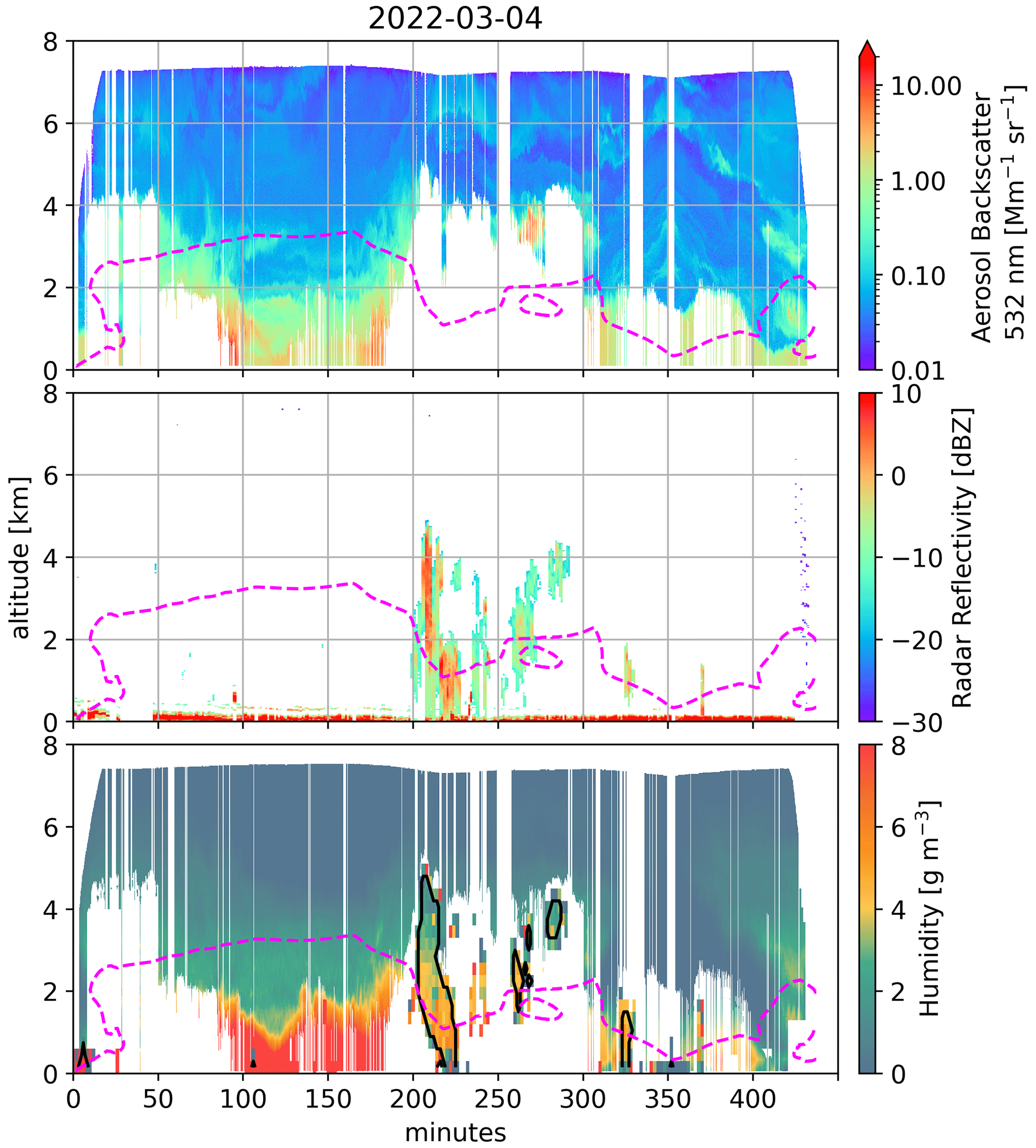
Figure 14 showcases the synergy of the lidar and radar measurements as well as the DIAL and DAR measurements. The top panels display the high spectral resolution lidar aerosol backscatter at 532 nm for the SOA²RSE flight on 8 and 9 March, while the middle panels show the VIPR radar reflectivities at 167.12 GHz. As shown, as the clouds thicken the lidar becomes insensitive to largest particles, while VIPR becomes sensitive to them. The bottom panels display curtain plots of the HALO and VIPR water vapor estimates for the flights on 8 and 9 March. (Similarly, Fig. A1 displays the 4 March flight; note that there were no cloudy measurements on the 7 March flight.)

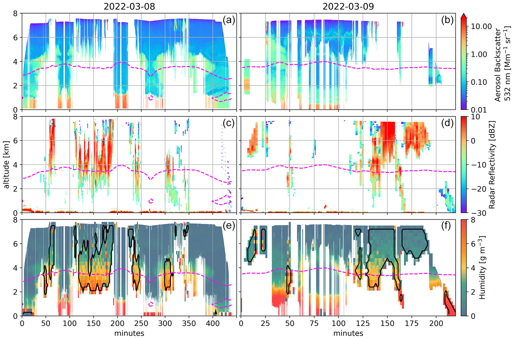
Figure 14 Panels (a) and (b) show 532 nm high-spectral-resolution lidar aerosol backscatter for the SOA²RSE flight on 8 and 9 March. Panels (c) and (d) show calibrated radar reflectivities at 167.12 GHz (also shown in Fig. 6), and (e) and (f) show VIPR and HALO humidity measurements. VIPR measurements are delimited by a black contour. Dashed magenta lines depict the melting layer.

The combined use of HALO and VIPR enables the estimate of high-resolution water vapor profiles in both clear-sky and in-cloud conditions. For example, on the 8 March flight, HALO can see in between the clouds (see around 90, 200, and 275 min into the flight), revealing elevated water vapor values (∼8 g m⁻³) in the planetary boundary layer (the first 1 km of the atmosphere), while next to it, VIPR indicates such elevated values up to around 3 km within the mid-level convection (see also Fig. 8, 8 March ERA5 panel).

To underscore the synergy of these techniques, Fig. 15 displays the normalized histograms of the water vapor values retrieved by either DIAL/HALO or DAR/VIPR. As shown, DAR/HALO displays a skewed right distribution with mode at 0.4 g m⁻³ (attributed to a majority of clear-sky measurements), while DAR/VIPR exhibits a multimodal broad distribution with modes at 0.8 and 4.4 g m⁻³. This synergy could provide insights into lower tropospheric clear-sky and in-cloudy turbulent transport processes enabling comparisons and improvements of regional models as well as large eddy simulations.

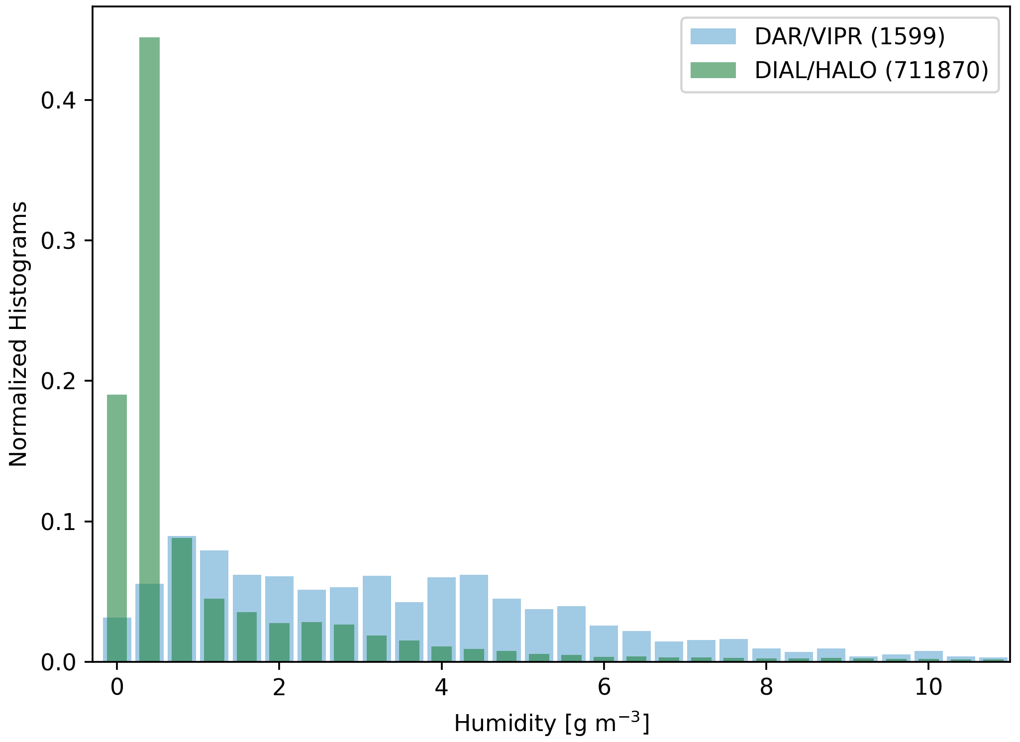
Figure 15 Normalized histogram of the humidity retrievals during the SOA²RSE 8 and 9 March flights using either DAR/VIPR or DIAL/HALO. The numbers in brackets represent the number of samples per instrument.

7 Conclusions

The VIPR G-band radar was deployed on the P-3 aircraft as part of the IMPACTS and SOA²RSE campaigns, encompassing a total of eight flights and collecting approximately 44 h of data. This provided the opportunity of evaluating the VIPR DAR water vapor estimates under two complete different weather regimes, that is, inside snowstorms (IMPACTS flights) and during calm weather (SOA²RSE flights).

For the first time, VIPR operated using three radar tones (158.6, 167.12, and 174.48), which allowed disentangling the differential extinction from the water vapor from the hydrometeor scattering and absorption effects. By using three frequencies instead of only two (as in previous VIPR configurations), biases were mitigated, ensuring more accurate and reliable water vapor estimations.

In this study, VIPR and ERA5 averaged to 10 min along track were intercompared and validated against dropsondes. These comparisons can be broken in three categories:

• In-cloud profile comparisons. During IMPACTS, VIPR and ERA5 agree within 20 % except at the moisture bands where ERA5 seems to underestimate the VIPR humidity measurements by up to 50 %. During SOA²RSE, ERA5 displays up to a 50 % underestimation of the VIPR estimates above ∼4 km.

  A scatterplot comparison against dropsondes suggests an overall good agreement with VIPR during both IMPACTS and SOA²RSE (with RMSD better than 0.55 g m⁻³ and an overall bias better than 0.05 g m⁻³) and an overall good agreement with ERA5 during IMPACTS (RMSD=0.13 g m⁻³ and $\text{bias}=-\mathrm{0.08}$ g m⁻³). During SOA²RSE, ERA5 shows a clear underestimation for water vapor (RMSD=0.69 g m⁻³ and $\text{bias}=-\mathrm{0.48}$ g m⁻³), in particular for estimates above ∼4 km. Breaking down this into biases versus altitude suggests that, during IMPACTS, VIPR humidity estimates agree within 10 % with the dropsondes through most heights, while ERA5 agrees within 10 % (or better). During SOA²RSE VIPR water vapor estimates agree within 20 % with the dropsondes through most heights, while ERA5 agrees within 20 % with the dropsondes below 4 km, but it displays an underestimation of up to 50 % above it, thus corroborating the VIPR and ERA5 intercomparison.

  Through these comparisons, it became evident that the VIPR retrieval may introduce some artifacts at the edges of clouds and snowstorms. Biases resulting from these artifacts can be mitigated either by using the median instead of the mean or by excluding water vapor estimates that deviate more than 3 standard deviations from the mean when averaging over the 10 min period employed in these comparisons.

• Clear-sky (ERA5 only) profile comparisons. During both IMPACTS and SOA²RSE, ERA5 shows overall good agreement against the dropsondes (with RMSD better than 0.72 g m⁻³, and an overall bias better than −0.05 g m⁻³) but displays large excursions from the one-to-one line. These excursions translate to large biases (up to 250 %) at particular heights. Since ERA5 agrees with the dropsondes in the in-cloud regimes, these clear-sky biases suggest that ERA5 is presumably failing to simulate the extent of the snowstorms. During SOA²RSE, ERA5 agrees with the dropsondes within 20 % below 5 km but displays an overestimation of up to 80 % above this altitude.

• pCWV comparisons. Overall, VIPR and ERA5 display a good agreement with the dropsonde pCWV estimates, with VIPR displaying an RMSD of 1.5 kg m⁻² and a bias of 0.6 kg m⁻², while ERA5 displays an RMSD of 1.8 kg m⁻² and a bias of −1 kg m⁻². These relatively high RMSD values are presumably due to the nature of the snowstorm scene. That is, dropsondes launched within 10 min of each other also display an RMSD of around 1.5 kg m⁻² with respect to their mean value. A direct comparison between the VIPR and ERA5 pCWV estimates indicates a possible ERA5 underestimation, in particular during the IMPACTS flights.

Lastly, the SOA²RSE campaign offered, for the first time, the opportunity to show the synergistic abilities of combining DIAL and DAR water vapor measurements, enabling the estimate of high-resolution water vapor profiles in both clear-sky and in-cloud conditions. Observations of water vapor in the planetary boundary layer from space are crucial for advancing our understanding of the dynamics in this critical atmospheric layer (National Academies of Sciences, Engineering, and Medicine, 2018). These airborne campaigns constitute an essential step toward transitioning DAR and DIAL to an orbital platform.

Appendix A

Figure A1 As Fig. 14 but displaying the 4 March flight.