the Creative Commons Attribution 4.0 License.
the Creative Commons Attribution 4.0 License.
 | 25 Sep 2024
Field assessments on the impact of CO2 concentration fluctuations along with complex-terrain flows on the estimation of the net ecosystem exchange of temperate forests
Dexiong Teng
Jiaojun Zhu
Fengyuan Yu
Yuan Zhu
Xinhua Zhou
Bai Yang
CO2 storage (Fs) is the cumulation or depletion in CO2 amount over a period in an ecosystem. Along with the eddy covariance flux and wind-stream advection of CO2, it is a major term in the net ecosystem CO2 exchange (NEE) equation. The CO2 storage dominates the NEE equation under a stable atmospheric stratification when the equation is used for forest ecosystems over complex terrains. However, estimating Fs remains challenging due to the frequent gusts and random fluctuations in boundary-layer flows that lead to tremendous difficulties in capturing the true trend of CO2 changes for use in storage estimation from eddy covariance along with atmospheric profile techniques. Using measurements from Qingyuan Ker Towers equipped with NEE instrument systems separately covering mixed broad-leaved, oak, and larch forest towers in a mountain watershed, this study investigates gust periods and CO2 fluctuation magnitudes and examines their impact on Fs estimation in relation to the terrain complexity index (TCI). The gusts induce CO2 fluctuations for numerous periods of 1 to 10 min over 2 h. Diurnal, seasonal, and spatial differences (P < 0.01) in the maximum amplitude of CO2 fluctuations (Am) range from 1.6 to 136.7 ppm, and these differences range from 140 to 170 s in a period (Pm) at the same significance level. Am and Pm are significantly correlated to the magnitude of and random error in Fs with diurnal and seasonal differences. These correlations decrease as CO2 averaging time windows become longer. To minimize the uncertainties in Fs, a constant [CO2] averaging time window for the Fs estimates is not ideal. Dynamic averaging time windows and a decision-level fusion model can reduce the potential underestimation of Fs by 29 %–33 % for temperate forests in complex terrain. In our study, the relative contribution of Fs to the 30 min NEE observations ranged from 17 % to 82 % depending on turbulent mixing and the TCI. The study's approach is notable as it incorporates the TCI and utilizes three flux towers for replication, making the findings relevant to similar regions with a single tower.
- Article
(7325 KB) - Full-text XML
-
Supplement
(5151 KB) - BibTeX
- EndNote


The accurate estimation of the net ecosystem exchange (NEE) of carbon dioxide (CO2) in forest ecosystems is crucial for a comprehensive understanding of the global carbon cycle. The eddy covariance (EC) technique has been widely used in forest ecosystems due to its capacity to directly measure the NEE with measurement conditions satisfying the underlying theory. The EC technique is based on a simplified mass conservation equation (after Reynolds averaging), given by
where Vm is the volume of dry air in the control volume; c is the CO2 mixing ratio; t is the time; h is the measurement height; u, v, and w denote the velocity components in the x, y, and z directions, respectively; and an overbar denotes Reynolds averaging. This equation conceptualizes the NEE within a control volume from the ground to the measurement height (h) while ignoring the horizontal turbulence term divergence (Feigenwinter et al., 2004). In this equation, term I is the CO2 storage (Fs) representing the change in the average CO2 concentration (hereafter [CO2]). Terms II, IIIa, IIIb, and IV represent the vertical turbulent flux (Fc); the vertical advection; the interface vertical mass advection, such as the evaporation process (Webb et al., 1980); and the horizontal advection, respectively.
Most flux measurements typically lack solutions for terms III and IV and can only estimate the NEE by summing Fc and Fs, and a significant number of sites even ignore Fs. Fs in the vertical gas column within a canopy can be substantial, requiring attention in NEE estimates (Aubinet et al., 2000). Fs contributes ∼ 60 % to nocturnal turbulent flux underestimation in forest ecosystems with “ideal” topography (McHugh et al., 2017). During atmospherically stable periods such as the early morning, sunset, and nighttime transitions, Fs has an especially significant impact on the NEE. For 30 min ecosystem carbon flux measurements, ignoring Fs would cause the NEE to be underestimated (Zhang et al., 2010). The Fs value typically ranges from −2 to −5 µmol m−2 s−1 in the early morning, and it is about 1–3 µmol m−2 s−1 after sunset for temperate forests. The effect of Fs on the NEE of forest ecosystems decreases with an increase in the timescale (Li et al., 2020). However, neglecting the Fs value can lead to misunderstanding the CO2 exchange processes, such as ecosystem respiration and photosynthesis, and their relationship with key control factors such as solar radiation, temperature, and moisture (McHugh et al., 2017). Therefore, it is imperative not to overlook Fs to ensure more precise NEE estimates of forest ecosystems, particularly in complex terrain.
Despite the challenges inherent in monitoring forest conditions, understanding the carbon flux of forest ecosystems in complex terrain or with heterogeneous underlying surfaces remains an area of great interest. Topography complexity plays a complex role in the transportation of momentum, energy, and mass in the atmospheric boundary layer, with direct impacts on airflow patterns, spatiotemporal characteristics, and gas concentration fluctuations (Sha et al., 2021; Finnigan et al., 2020). Differences in airflow along a slope, lateral CO2 discharge downhill, and spatiotemporal variations in soil respiration result in the CO2 outflow from slopes and valleys lagging behind the flat tops of mountains (de Araújo et al., 2010). At night, under stable atmospheric stratification, cold air moves from the valley forest canopy to the ground and then flows to low-lying areas, causing a “carbon pooling” effect. The gradient of [CO2] below the EC sensors fluctuates significantly, and the cold-air discharge above the canopy reduces CO2 storage, leading to an underestimation of forest ecosystem respiration (Yao et al., 2011; de Araújo et al., 2008, 2010).
According to the theoretical definition, Fs estimates are derived by averaging the [CO2] of the control volume at the beginning and the end of the EC averaging period (30 min or 1 h) and dividing this by the EC averaging period (Finnigan, 2006). The estimation of Fs at numerous sites frequently employs a vertical profile system. This approach operates under the assumption that Fs represents the integration of the time derivative of the vertically determined column-averaged [CO2]. It is noteworthy that the column-averaged [CO2] may not accurately represent the average [CO2] of the control volume in cases of inadequate air mixing, leading to insufficient sampling. A previous study showed that relying solely on tower-top measurements can lead to the underestimation of Fs by up to 34 % compared to using an eight-level profile approach (Gu et al., 2012). The NEE magnitude with Fs based on a 2 min [CO2] averaging time window (instantaneous-concentration approach) was found to be 5 % higher than that with Fs based on a 30 min window (averaging-concentration approach), particularly during the nighttime in the growing season (Wang et al., 2016). A proper measuring system that improves horizontal representativeness can reduce the bias in Fs to 2 %–10 % (Nicolini et al., 2018). Most research has examined how the vertical and horizontal gas concentration sampling point distribution affects the uncertainty in Fs estimation (Bjorkegren et al., 2015; Wang et al., 2016; Yang et al., 2007, 1999), with a small number of studies examining the effect of [CO2] sampling frequency on Fs (Finnigan, 2006; Heinesch et al., 2007). Certain studies have experimentally validated new concepts, such as correlating the gas sampling point concentration with the horizontal distribution (Nicolini et al., 2018). Some studies have approached the true value theoretically, such as through defining the control volume represented by flux measurements (Metzger, 2018; Xu et al., 2019). However, the number of complete column samples required to describe the column-averaged [CO2] of each 30 min or 1 h Fs estimate is still undetermined.
Previous studies have emphasized the significance of Fs to the NEE and the influence of [CO2] dynamics on Fs estimates in complex terrain. To overcome any disparities between sensors and obtain precise changes in the [CO2] gradient above and below the forest canopy, individual gas analyzers are extensively utilized to measure [CO2] levels vertically (Siebicke et al., 2011). However, a single gas analyzer introduces time delays when monitoring multi-point [CO2] curves. Accurately determining the Fs estimates can be challenging due to the spatial and temporal resolution of [CO2] measurements (Wang et al., 2016). The random error in the Fs estimates using one complete column sample is considerably high due to short-term [CO2] fluctuations (Nicolini et al., 2018). The calculation of Fs using time-averaged [CO2] profiling leads to significant information loss at a high frequency, resulting in a substantial underestimation bias. Furthermore, time-averaged [CO2] profiling is employed to represent the [CO2] average within the control volume due to resource constraints. This leads to the systematic bias and random error in Fs estimates being irreconcilable. This issue necessitates further efforts to characterize [CO2] fluctuations across different sites and to demonstrate the mechanisms influencing Fs magnitudes, Fs uncertainties, and their contributions to NEE observations in complex terrain. Thus, this study aims to bridge this gap by introducing a statistical method to estimate Fs values and their uncertainties.
This paper employs an innovative EC experimental setup with three flux towers (Qingyuan Ker Towers) to monitor three typical types of temperate forest stands located in complex terrain in northeastern China. This study introduces a decision-level fusion model based on weighting the underestimation bias and random error in Fs to obtain more accurate results. The objectives of this study were to (1) compare diurnal, seasonal, and spatial differences in [CO2] fluctuations, Fs, and its uncertainty; (2) examine the variation in Fs uncertainty with different [CO2] averaging time windows; and (3) investigate the response of Fs and its uncertainty to [CO2] fluctuations, wind above the canopy, and terrain complexity, quantifying the impact of Fs on the NEE estimates under these conditions.
2.1 Study site and instrumental setup
This study was conducted in temperate forests in a watershed based on Qingyuan Ker Towers (Zhu et al., 2021; Gao et al., 2020), situated in northeast China (41°50′ N, 124°56′ E). The region experiences a temperate continental monsoon climate, with an average annual temperature of 4.3 °C and annual rainfall of 758 mm from 2010 to 2021 (Li et al., 2023). Qingyuan Ker Towers consist of three 50 m high EC towers (Fig. 1) that observe a mixed broad-leaved forest (MBF), a Mongolian oak forest (MOF), and a larch plantation forest (LPF).
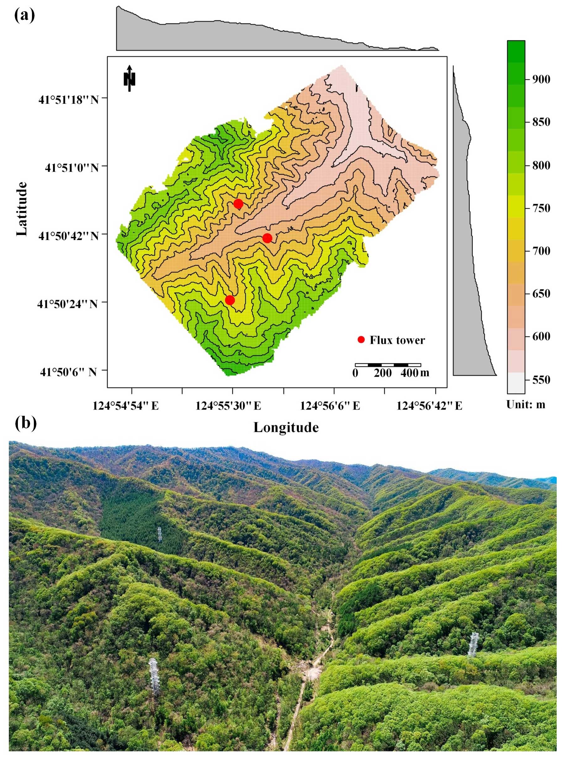
Figure 1Overview of the study area. Panel (a) depicts the topography of the study site, with black curves indicating elevation contours and marginal distributions represented as a gray graph, averaged over rows and columns. Panel (b) features an aerial photograph of Qingyuan Ker Towers captured in the growing season (Gao et al., 2020).
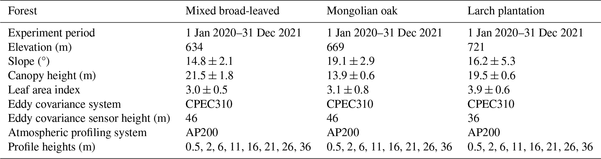
Basic information regarding Qingyuan Ker Towers in this study is presented in Table 1. The CPEC310 integrated system from Campbell Scientific, comprising an EC155 closed-path infrared gas analyzer (IRGA) and a CSAT3A sonic anemometer, was employed to monitor the three-dimensional wind speed and CO2 and H2O concentrations (10 Hz). An atmospheric profiling system (AP200, Campbell Scientific, Inc., Logan, UT, USA) was utilized to measure the CO2 and H2O concentrations with eight height levels. Each level was measured for 15 s (with 10 s for the flushing of the manifold and 5 s for logging the average), leading to a measurement cycle of 2 min. Due to calibration, filter changes, and rugged weather, 10 % of CPEC310 data and 3 % of AP200 data were missed in our study period.
2.2 Calculation of storage flux
Averaging [CO2] in a time window was utilized to calculate the Fs values, in addition to data on the air pressure, CO2 and H2O molar fractions, and air temperature at different heights above the ground surface (Finnigan, 2006; Montagnani et al., 2018; Xu et al., 2019). The molar mixing ratio and mass mixing ratio are quantities conserved with the variation in air temperature, air pressure, and water vapor concentration, whereas the molar fraction is not. This study determined Fs using the molar mixing ratio obtained from CO2 and H2O molar fraction observations, applying the ideal gas law and Dalton's partial pressure law (Montagnani et al., 2009). The water vapor molar mixing ratio (χv) in mmol mol−1 is given by
where cv is the water vapor molar fraction in mmol mol−1. The CO2 molar mixing ratio (χc) in µmol mol−1 is given by
where cc is the CO2 molar fraction in µmol mol−1.
The dry air density () in mol m−3 is calculated as follows:
where R∗ is the air gas constant (8.31441 Pa m3 K−1 mol−1), is the air pressure in pascals, and is the average air temperature in degrees Celsius. Md and Mv are the dry air and water vapor molar mass (18.015 g mol−1), respectively. Md is calculated from the CO2 molar mixing ratio (Khélifa et al., 2007):
where Mc is the carbon molar mass (12.011 g mol−1).
The Fs values estimated from eight-level profiles are calculated as follows:
where is the average CO2 molar mixing ratio and Δhi is the height represented by each level.
When measuring Fs by sampling CO2 at several levels using a single analyzer, synchronous observations of the CO2 profile are impractical. Consequently, discrete temporal sampling and time averaging become necessary. To ensure the temporal alignment of Fs with Fc, the average [CO2] measurements within the control volume at the beginning and end (t) of an averaging period (30 min) are calculated by averaging over a time window (τ min) as follows:
where τ = 4, 8, …, 28 min. Theoretically, the time window should be kept as short as possible in comparison to the turbulence flux averaging period to comply with the principle of Reynolds decomposition. We use large windows here for CO2 averaging in an attempt to demonstrate the effects of different window sizes on the accuracy of storage flux estimates.
2.3 Data analysis
To evaluate the impact of [CO2] fluctuations on Fs measurements and corresponding uncertainty, empirical modal decomposition (EMD) and Fourier spectrum analysis (FSA) were used to extract the period and amplitude of fluctuations in the high-frequency [CO2] time series (10 Hz). EMD was used to decompose the [CO2] time series into intrinsic mode functions based on local signal properties (Huang and Wu, 2008), which yielded instantaneous frequencies as functions of time and allowed for the identification of embedded structures of eddies. EMD is applicable to nonlinear and nonstationary processes (Huang et al., 1998). The period and amplitude of [CO2] fluctuations above the forest canopies reflected the eddy size. Subsequently, the maximum period and amplitude of [CO2] fluctuations in the short term (2 h) were indicative of large eddies under the influence of gusts.
Due to the diurnal and seasonal variability in flux measurements, this study defined the transition period and growing season. The solar elevation angle was used to define the transition period as 1 h before sunrise (sunset) to 2 h after sunrise (sunset). The growing degree days (GDDs) were calculated using the base temperature (Tbase) to determine the beginning and end of the growing season, and the formula for this was as follows (McMaster and Wilhelm, 1997):
where Tbase is 6 °C. Considering the persistent need for temperature levels to support vegetation growth, the fourth day of the first GDD greater than zero (less than zero) over a span of 5 consecutive days was defined as the starting (ending) time of the growing season.
The main data processing and analysis steps are outlined below:
-
EMD and Fourier spectrum analysis of [CO2] high-frequency time series were used to extract the maximum amplitude (Am) and corresponding period (Pm) of [CO2] fluctuations every 2 h. The data were divided into two subsets based on Pm, with a cutoff of 150 s.
-
CO2 storage fluxes were calculated for different [CO2] averaging time windows (τ), ranging from 4 to 28 min in increments of 4 min.
-
The standardized major axis (SMA) regression model (Warton et al., 2012) was used to compare the slope differences (bias) between Fs_τ and Fs_28 for different Pm values and the forest stands. The SMA model offers routines for comparing parameters a and b among groups for symmetric problems.
-
The normalized root mean square error (NRMSE) and slope were used to evaluate the relative error and bias between Fs_τ and Fs_28. The NRMSE is calculated as
where i indicates the ith observation.
-
The normalized weighting coefficient (w) of Fs_τ was estimated based on the NRMSE and slope (Wang et al., 2020). Details are shown in Appendix A1. Then, using the decision-level fusion model, Fs_comb was calculated as
The decision-level fusion model automatically assigned weights to Fs based on different [CO2] averaging time windows. Its purpose in this study was to balance the relative error and bias in Fs estimates caused by [CO2] sampling. The analysis was performed using the EMD and smatr R packages (Warton et al., 2012; Huang et al., 1998).
2.4 Uncertainty analysis
To improve the accuracy of estimating the uncertainty in Fs using an individual tower, this work has made modifications to the 24 h difference method by extending the sampling time windows and applying meteorological-condition constraints (Hollinger and Richardson, 2005). This method trades time for space to estimate the uncertainty in Fs. To determine the uncertainty in Fs, expressed as σ(εs), in this case, we compared the observations at moment i within a day to the average of several observations during a similar period and with similar meteorological conditions. The specific computations were as follows:
where Ω is the moment interval (i−0.5 h, i+0.5 h) within a certain time window (15 d); I is the indicator function; the set represented by Λ consisted of elements that meet similar meteorological conditions, including u∗, air temperature (Ta), and sensible heat flux (H); , , and σH are the standard deviation of u∗, Ta, and H, respectively; δ is the threshold of Euclidean distance; and εs is the random error in Fs.
After estimating the uncertainty in Fs, this study extended the work conducted by Richardson et al. (2008) to analyze its relationship with the magnitude of flux measurements (), [CO2] fluctuations (Am and Pm), u∗, and the terrain complexity index (TCI). A comprehensive description of the TCI can be found in Appendix A2. This relationship can be approximated using the following equation:
where the nonzero intercept term β0 indicates the size of the random uncertainty as xi approaches 0, which varies with the observation site, with larger values of β0 indicating greater uncertainty. The slope term βi indicates the sensitivity of the size of the random uncertainty in xi, with smaller βi values indicating a probability distribution of uncertainty closer to white noise.
3.1 Characterization of [CO2] fluctuation and Fs variations
The high-frequency [CO2] time series above the forest canopies were decomposed using EMD, and this was followed by spectral analysis to extract the fluctuation period and amplitude of [CO2] on different timescales. As depicted in Fig. 2, it became evident that the [CO2] above the canopies displayed short-term fluctuations with periods ranging from 1 to 10 min, and the amplitude of these fluctuations showed an increasing trend with longer periods. This observation strongly suggests the presence of large eddies influenced by gusts above the canopies, and these eddies were responsible for the increasing amplitude of [CO2] fluctuations as their size increased.
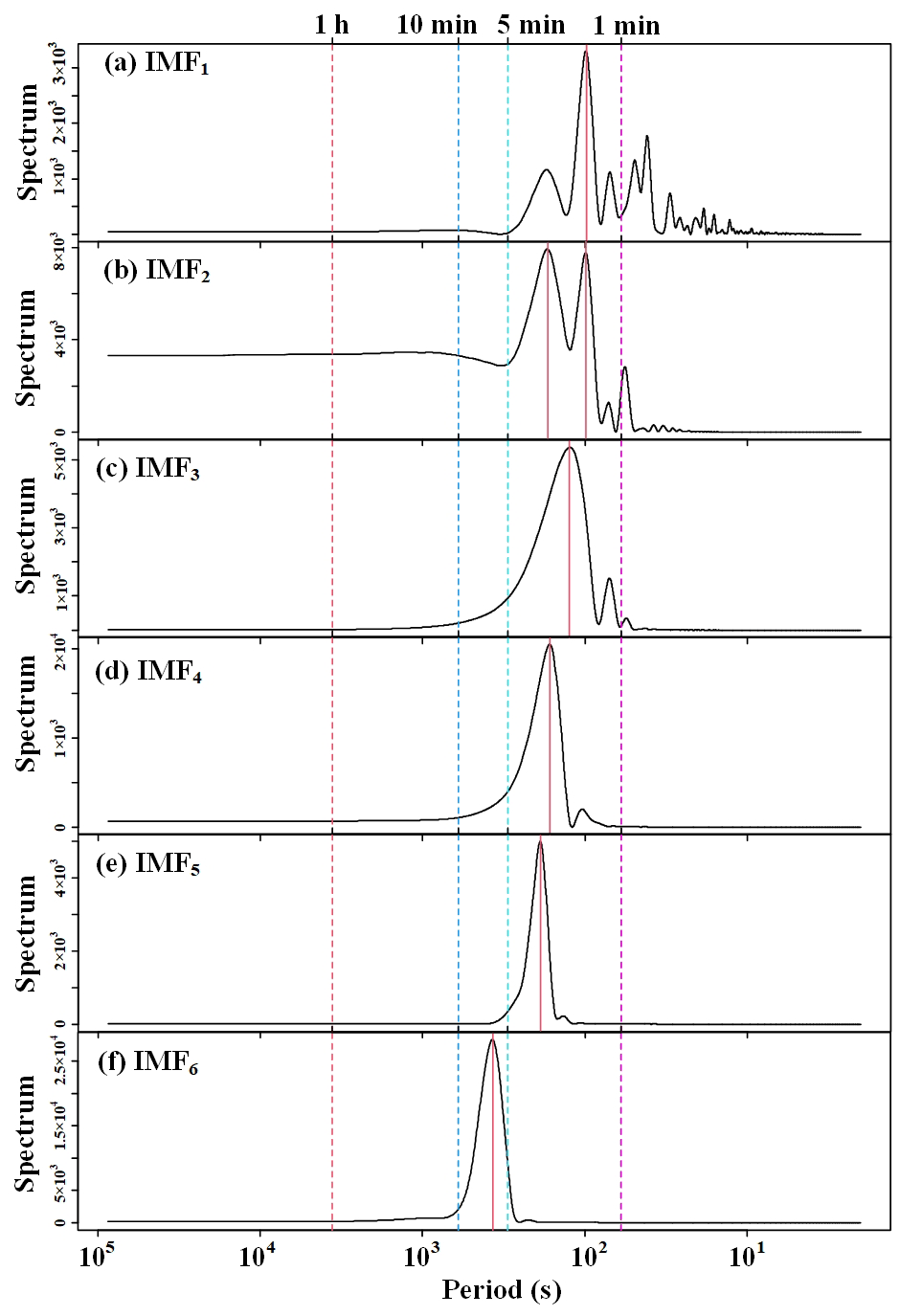
Figure 2Power spectral density of the intrinsic mode function (IMF) of above-canopy CO2 concentrations in the Mongolian oak forest on 2 July 2020 (24 h).
Table 2The means of Am in parts per million (ppm) and Pm in seconds (s) for three forest stands in different periods.
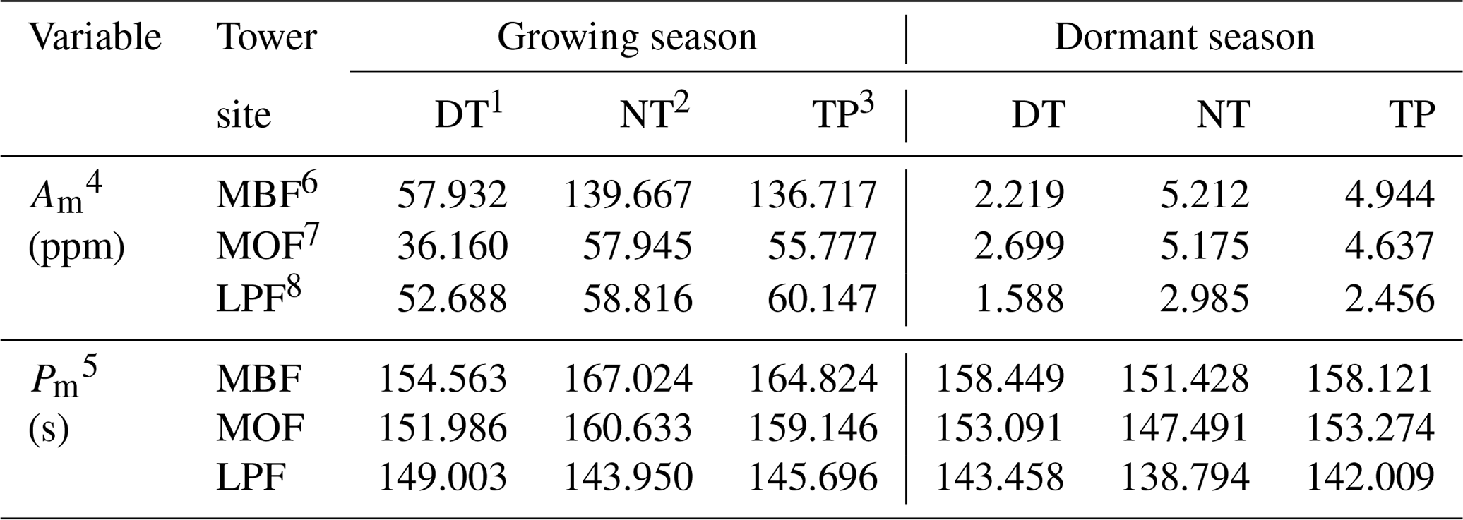
1 DT represents daytime. 2 NT represents nighttime. 3 TP represents the transition period. 4 Am represents the maximum amplitude of short-term CO2 concentration fluctuations. 5 Pm represents the corresponding period of maximum amplitude. 6 MBF represents mixed broad-leaved forest. 7 MOF represents Mongolian oak forest. 8 LPF represents larch plantation forest.
To examine the spatiotemporal variations in large eddies, this study compared the Am and Pm values above canopies across different forest stands. The analysis utilized data from daytime, nighttime, and transition periods in both the growing and the dormant seasons. The averages of Am and Pm for the above-canopy [CO2] in the three forest stands ranged from 1.588 to 136.667 ppm and from 2.313 to 2.784 min, respectively (Table 2). Figure 3 demonstrates significant seasonal and diurnal differences (P < 0.01) in Pm, with higher values during the daytime in the growing season and lower values during the daytime in the dormant season. Moreover, Pm was significantly different (P < 0.01) among different forest stands during the same time period, with the MBF stand having the highest values, followed by MOF and then LPF with the lowest values. During the growing season, the Am values were significantly higher than those during the dormant season, with both daytime and nighttime values also exhibiting significant differences (P < 0.01) among different forest stands. This observation provides evidence of significant spatiotemporal variability in the large eddies influenced by gusts.
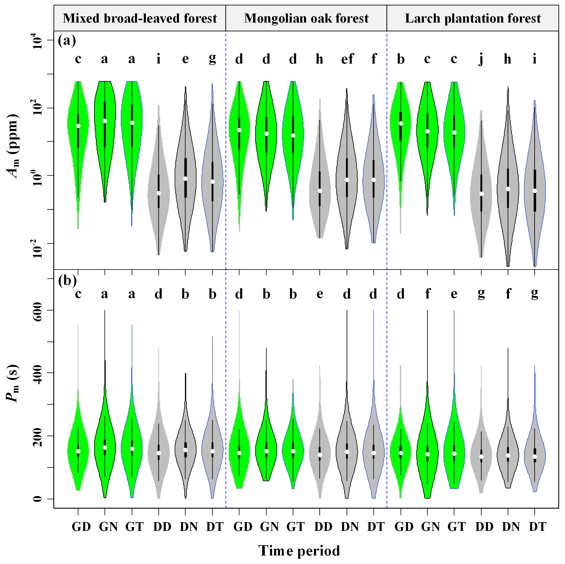
Figure 3The maximum amplitude (Am) (a) and corresponding period (Pm) (b) of short-term CO2 concentration fluctuations in different forest stands for seasonal and diurnal variations, where GD, GN, GT, DD, DN, and DT denote the growing-season daytime, growing-season nighttime, growing-season transition period, dormant-season daytime, dormant-season nighttime, and dormant-season transition period, respectively. Columns with different lowercase letters are significantly different (P < 0.05) according to Fisher's least significant difference test.
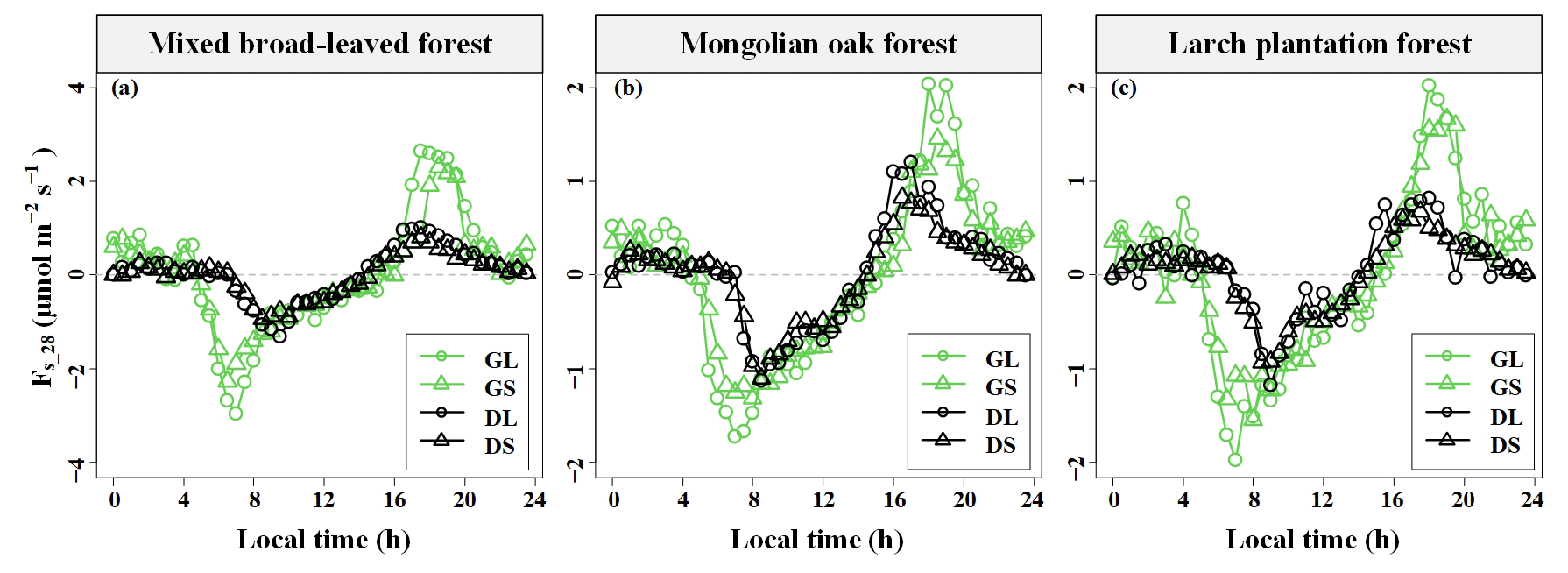
Figure 4Median diurnal variation in CO2 storage flux (Fs) based on 28 min CO2 concentration averaging time windows in the three forest stands during different seasons. GS indicates the growing season and a short period of maximum amplitude (Pm), GL indicates the growing season and a high Pm, DS indicates the dormant season and a low Pm, and DL indicates the dormant season and a high Pm (the L in the abbreviations is derived from long and the S from short).
To estimate the uncertainty in Fs using an individual tower, a comprehensive analysis of the diurnal and seasonal dynamics, as well as the functional relationship between Fs and u∗, was necessary. Significant diurnal variations and seasonal differences in Fs were observed across the three forest stands, as shown in Fig. 4. During the growing season, the median diurnal variation in Fs for the three forest stands ranged from −2.960 to 2.647 µmol m−2 s−1, whereas during the dormant season, it ranged from −1.306 to 1.012 µmol m−2 s−1. Comparing the extent of Fs diurnal variation among the three forest stands, MBF exhibited the largest extent during the growing season, while the extents of the three forest stands were similar during the dormant season. Notably, it was observed that the amplitudes for higher Pm values were greater than those for lower Pm values. This observation indicates that the larger the eddies, the greater the magnitude of Fs.
Furthermore, a u∗ threshold value was identified for the variation in Fs with u∗ during the daytime in both the dormant and the growing seasons (Fig. 5). When u∗ fell below the u∗ threshold, the magnitude of Fs () decreased with increasing u∗. Conversely, when u∗ exceeded the u∗ threshold, tended to remain relatively constant. Notably, a maximum point for was observed when u∗ was less than 0.5 m s−1 during the growing season, whereas this was not the case during the dormant season. This phenomenon was particularly evident during the nighttime and transition periods of the growing season, when exhibited an initial increase followed by a subsequent decrease with u∗. These observations strongly indicate that the effect of the turbulent mixing strength on over complex terrain is nonlinear and exhibits diurnal and seasonal differences.
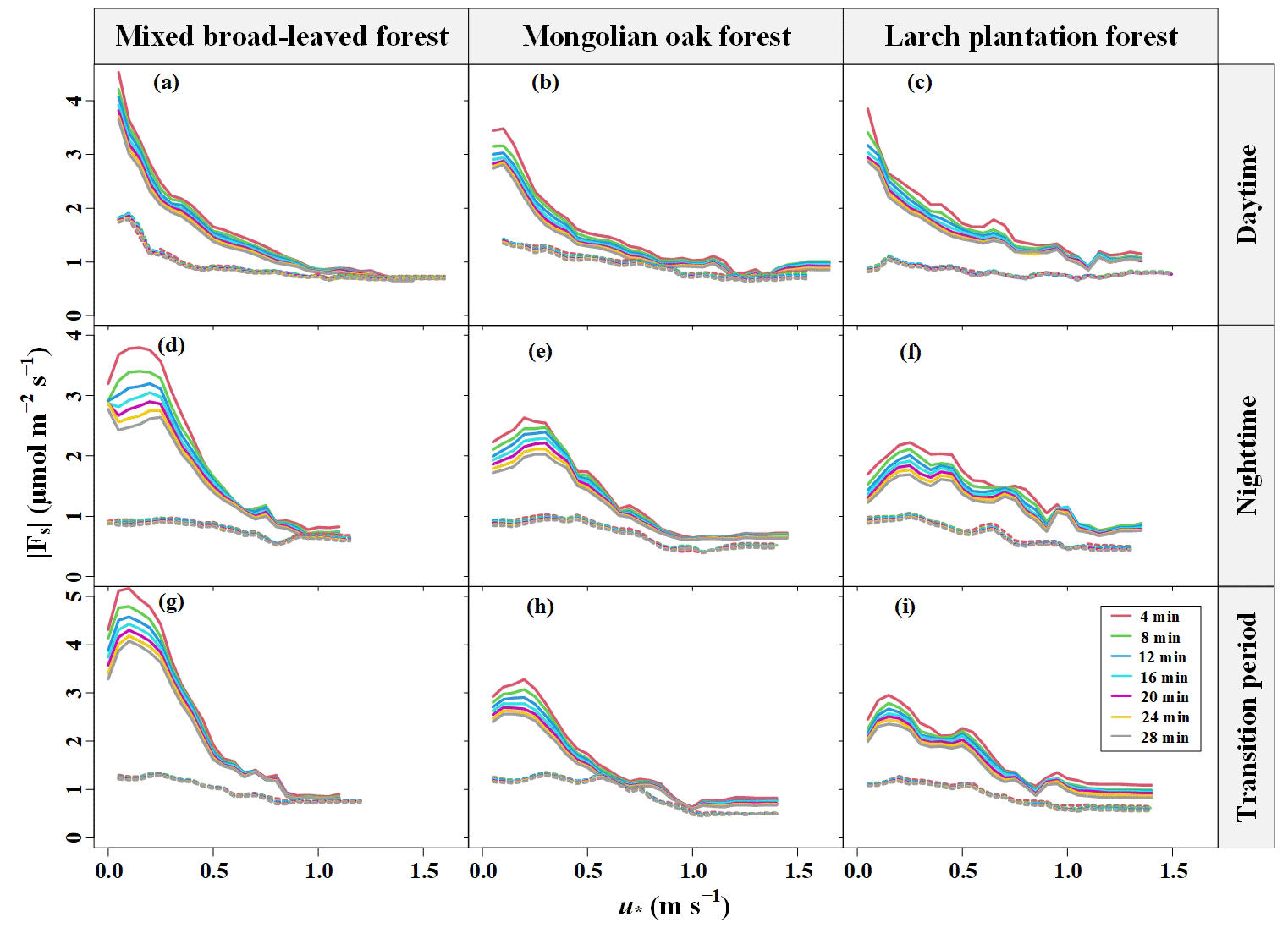
Figure 5Magnitudes of CO2 storage flux () determined with different CO2 concentration averaging time windows as a function of the friction velocity (u∗) and moving-block averages from all 30 min data for the years 2020–2021. Dashed and solid lines indicate the dormant and growing seasons, respectively.
3.2 Effect of [CO2] fluctuations on Fs and its uncertainty
To investigate the influence of the [CO2] fluctuation periods on the error in Fs measurement, this study computed the diurnal average of the standard deviation σ(εs) of the 30 min Fs uncertainty (εs) separately for different Pm values and the seasons. The overall distribution of εs showed a non-normal distribution with a high peak (kurtosis > 2 and P < 0.05; results presented in Tables S1–S4 in the Supplement). The daily variation curves of σ(εs) in various [CO2] averaging time windows are presented in Fig. 6. It was observed that the diurnal-variation range of σ(εs) was higher during the growing season compared to the dormant season, regardless of the Pm lengths, indicating a seasonal difference independent of Pm. Additionally, during the growing season, both MBF and MOF demonstrated evident diurnal variation in σ(εs), with the peak occurring at night and the trough during the daytime. The diurnal-variation range of σ(εs) varied across the three forest stands, with MBF exhibiting the largest amplitude.
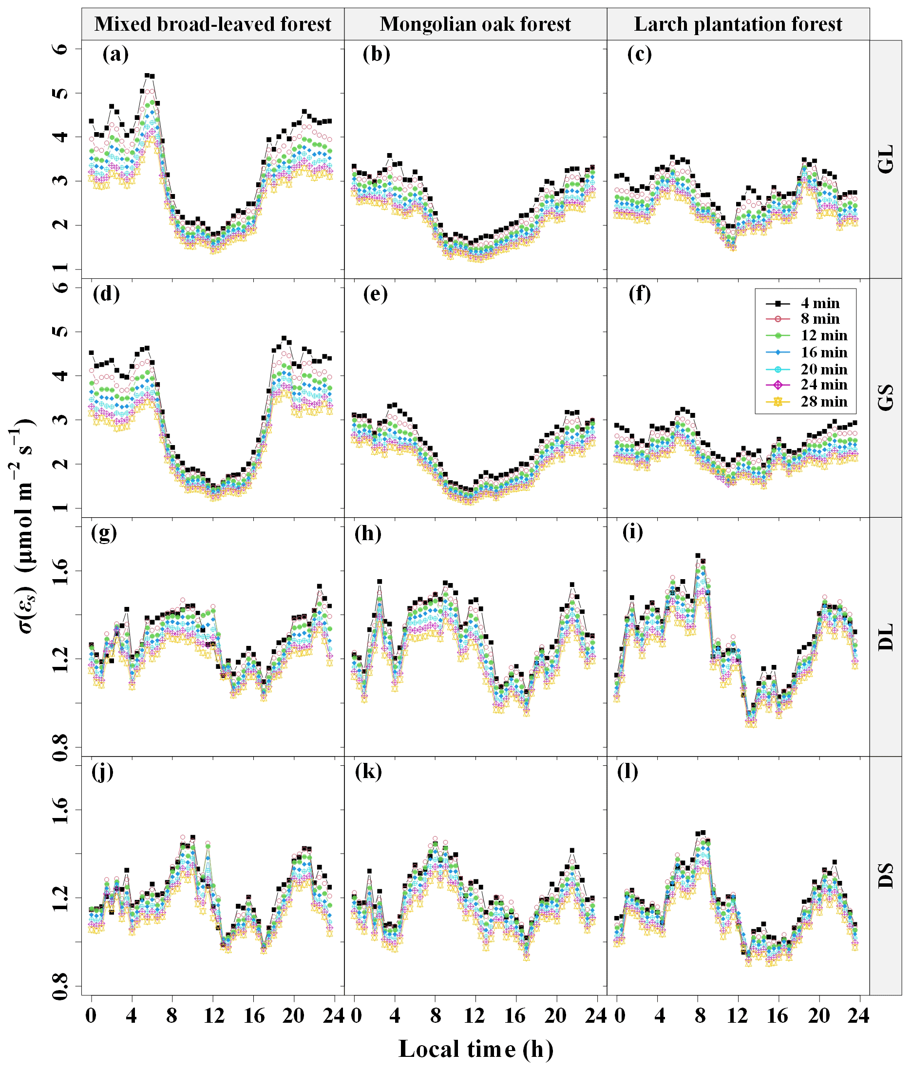
Figure 6Diurnal variations in the random uncertainty (σ(εs)) of CO2 storage flux (Fs) errors (εs) in different CO2 concentration ([CO2]) averaging time windows and their seasonal differences, where GS indicates the growing season and a short period of maximum amplitude (Pm) of [CO2] fluctuations, GL indicates the growing season and a high Pm, DS indicates the dormant season and a low Pm, and DL indicates the dormant season and a high Pm (the L in the abbreviations is derived from long and the S from short).
Furthermore, a significantly positive correlation was observed between σ(εs) and (P < 0.01), with site, seasonal, and diurnal differences (Fig. 7). The relationship between σ(εs) and was characterized by intercepts and slopes ranging from 1.99 to 2.82 µmol m−2 s−1 and from 0.24 to 0.28, respectively (results presented in Tables S5–S6). Both decreased as the [CO2] averaging time window increased, with the growing season exhibiting larger values compared to the dormant season (results shown in Tables S5 and S6). These findings suggest that increasing the [CO2] averaging time window results in a reduction in the random error in Fs and the correlation coefficient between σ(εs) and . This indicates a decrease in variability in σ(εs) and behavior similar to white noise.

Figure 7Random uncertainty σ(εs) in CO2 storage flux (Fs) errors (εs) in different CO2 concentration ([CO2]) averaging time windows as a function of the Fs magnitude for mixed broad-leaved forest, Mongolian oak forest, and larch plantation forest during the growing and dormant seasons. GS indicates the growing season and a short period of maximum amplitude (Pm) of [CO2] fluctuations, GL indicates the growing season and a high Pm, DS indicates the dormant season and a low Pm, and DL indicates the dormant season and a low Pm (the L in the abbreviations is derived from long and the S from short).
To assess the impact of [CO2] fluctuations on the error and bias in Fs measurement, this study compared the NRMSE and slopes of Fs based on different [CO2] averaging time windows, with reference to the baseline Fs_28, across various Pm values, time periods, and sites. As shown in Fig. 8, the NRMSE decreased and approached convergence as the [CO2] averaging time windows increased. During both the daytime and the nighttime in the growing season, the NRMSE corresponding to higher Pm was greater than that corresponding to lower Pm, while the opposite trend was observed during the dormant season. Additionally, the longer the [CO2] averaging time window, the greater the relative underestimation of Fs.
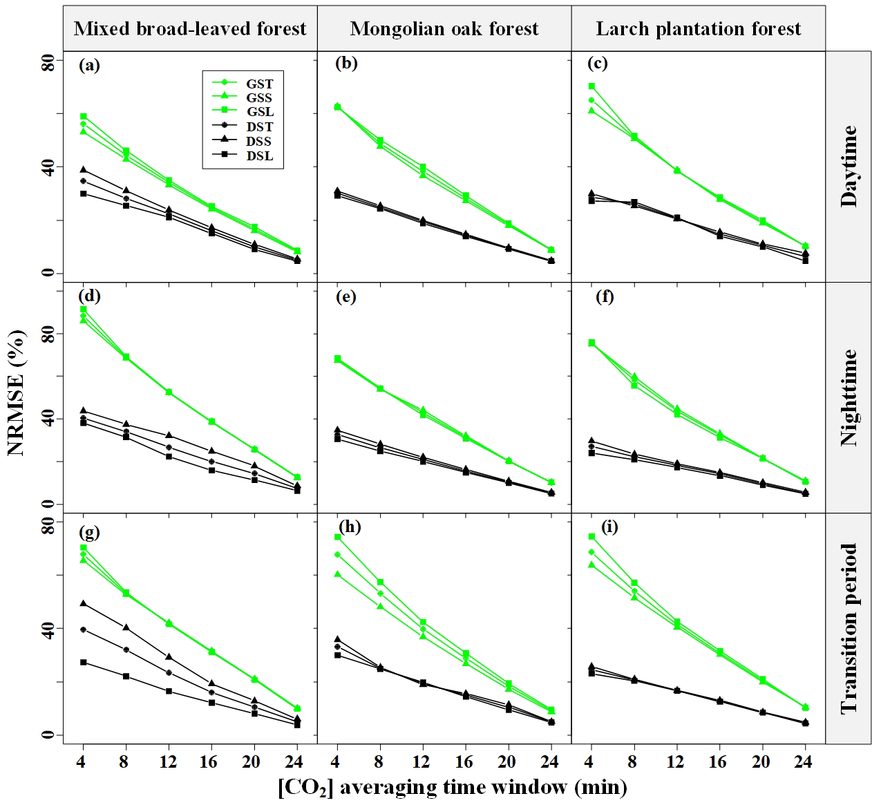
Figure 8Seasonal and diurnal differences in the normalized root mean square error (NRMSE) of CO2 storage flux (Fs) versus the respective Fs_28 values for different CO2 concentration ([CO2]) averaging time windows. GST indicates the growing season and does not distinguish the period of maximum amplitude (Pm) of [CO2] fluctuations, GSS indicates the growing season and a low Pm, GSL indicates the growing season and a high Pm, DST indicates the dormant season and does not distinguish Pm, DSS indicates the dormant season and a low Pm, and DSL indicates the dormant season and a high Pm (the L in the abbreviations is derived from long and the S from short).
A comparison of slopes between Fs_4 and Fs_28 in the three forest stands revealed interesting patterns, as depicted in Fig. 9. During the growing season, the slopes corresponding to the lower Pm of [CO2] fluctuations were consistently lower than those for the higher Pm, indicating that the effect of Pm on Fs uncertainty decreased with increasing [CO2] averaging time windows. However, for the MBF stand (Fig. 9d and g), the slopes corresponding to the lower Pm of [CO2] fluctuations during the dormant-season nighttime were actually greater than those for the higher Pm, primarily due to diurnal variations in the daily dynamics of Fs. Overall, the influence of Pm on Fs uncertainty decreased with increasing [CO2] averaging time windows. This suggests that averaging [CO2] reduced the effect of gusts on the random uncertainty in estimating Fs but led to a systematic underestimation of Fs.
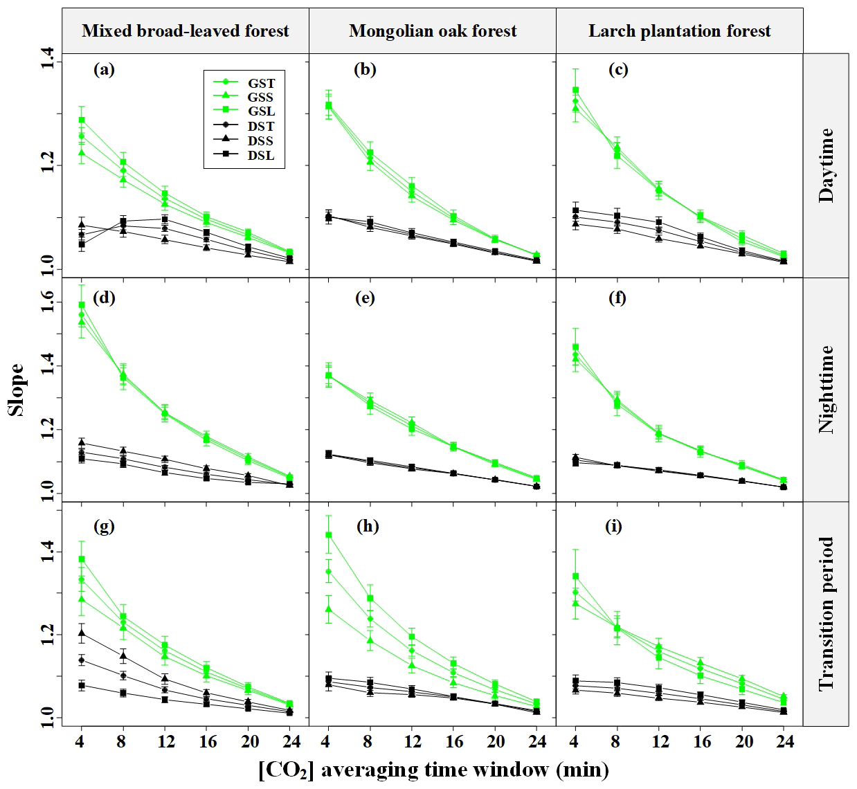
Figure 9Seasonal and diurnal differences in the slope of CO2 storage flux (Fs) versus Fs_28 for the different CO2 concentration ([CO2]) averaging time windows. GST indicates the growing season and does not distinguish the period of maximum amplitude (Pm) cases, GSS indicates the growing season and a low Pm, GSL indicates the growing season and a high Pm, DST indicates the dormant season and does not distinguish Pm, DSS indicates the dormant season and a low Pm, and DSL indicates the dormant season and a high Pm (the L in the abbreviations is derived from long and the S from short).
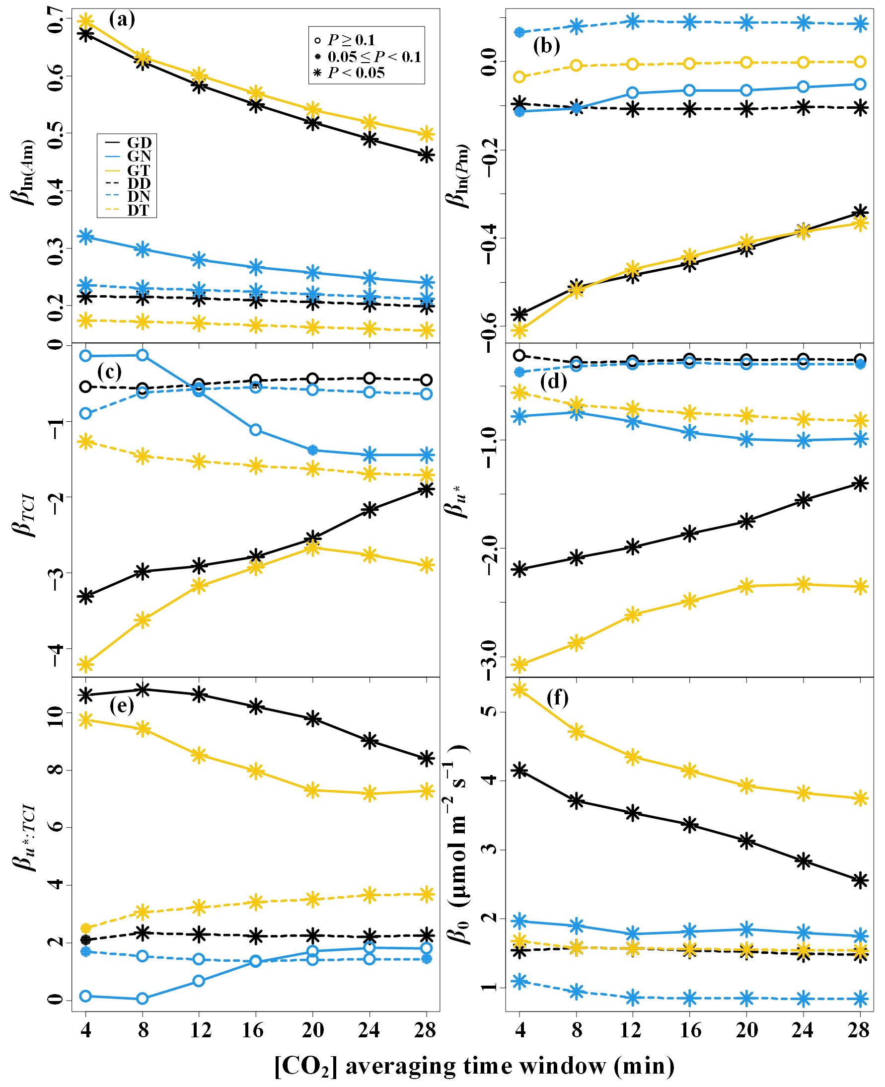
Figure 10Linear regression coefficients of the CO2 storage flux (Fs) magnitude – driving-factor relationships for the seven CO2 concentration ([CO2]) averaging time windows. The predictors of the multiple linear models are (a) the logarithm of maximum amplitude of [CO2] fluctuations (ln (Am)), (b) the logarithm of the corresponding period of maximum amplitude (ln (Pm)), (c) the terrain complexity index (TCI), (d) the friction velocity (u∗), and (e) the interaction term of the TCI and u∗. (f) β0 represents the intercept term.
To analyze the effect of [CO2] fluctuations on in complex terrain, this study developed a multiple linear regression model, considering the interaction effects of turbulent mixing and terrain complexity on , as shown in Fig. 10. Am exhibited a significant positive correlation with in all time periods (P < 0.05). Conversely, Pm showed a significant negative correlation with during the dormant-season daytime, the growing-season daytime, and the transition periods (P < 0.05). Additionally, their correlation coefficient decreased with increasing τ. In Fig. 10d and e, a u∗ threshold is observed during the growing-season nighttime. When u∗ was below the threshold, higher TCI values resulted in smaller values, whereas when u∗ was above the threshold, higher TCI values led to larger values. During the growing-season nighttime and transition periods, u∗ showed a significant negative correlation (P < 0.05) with , and the correlation coefficient decreased with increasing TCI values. These observations suggest that the effect of turbulent mixing on the uncertainty is regulated by terrain complexity.
A multiple linear regression model was used to analyze the effect of [CO2] fluctuations on the random uncertainty in Fs, σ(εs), in complex terrain. This model considered the interaction effects of [CO2] fluctuations and terrain complexity on σ(εs), as shown in Fig. 11. As evident from Fig. 11a and e, Am exhibited a significant positive correlation (P < 0.05) with σ(εs) during both the dormant season's nighttime and the growing season. Throughout the transition period of the growing season, Pm displayed a significant negative correlation with σ(εs) (P < 0.05). The magnitude of these correlation coefficients decreased with the increasing [CO2] averaging time windows. During the transition period of the dormant season, a TCI threshold was observed, with Pm showing a significant positive correlation (P < 0.05) with σ(εs) when the TCI was below the threshold and a significantly negative correlation (P < 0.05) with σ(εs) when the TCI exceeded the threshold (Fig. 11b and f). The u∗ value showed a significantly negative correlation with σ(εs) during the daytime and transition periods of the growing season (P < 0.05), while in other time periods, u∗ was significantly positively correlated with σ(εs) (P < 0.05). demonstrated a significant positive correlation with σ(εs) (P < 0.05) in all time periods, with its correlation coefficient being greater during the growing season than during the dormant season. These observations suggest that the relationship between the random uncertainty in Fs and [CO2] fluctuations is moderated by topographic complexity. Increasing the [CO2] averaging time window reduces the effect of [CO2] fluctuations on the random uncertainty in Fs.
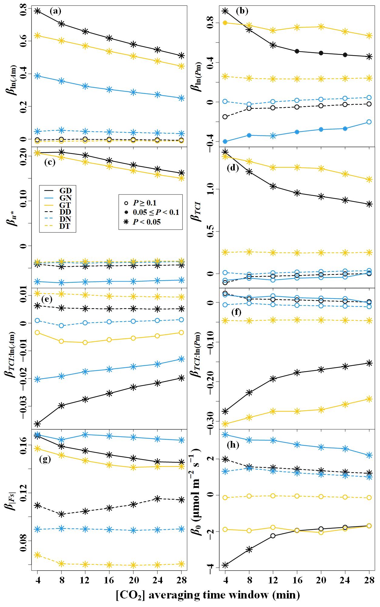
Figure 11Linear regression coefficients of the random uncertainty in CO2 storage flux (σ(εs)) – driving-factor relationships determined with Eq. (11) for the seven CO2 concentration ([CO2]) averaging time windows. The predictors of the multiple linear models are (a) the logarithm of maximum amplitude of [CO2] fluctuations (ln (Am)), (b) the logarithm of the corresponding period of maximum amplitude (ln (Pm)), (c) the friction velocity (u∗), (d) the terrain complexity index (TCI), (e) the interaction term of the TCI and ln (Am), (f) the interaction term of the TCI and ln (Pm), and (g) the magnitude of storage flux (). (h) The intercept term is represented by β0.
3.3 Effect of CO2 storage flux uncertainty in NEE observations
The 30 min Fs_comb was obtained by weighting the bias and random error in Fs using different [CO2] averaging time windows and Pm values. This study then focused on the magnitude of Fs_comb in relation to the Fc magnitude and its diurnal, seasonal, and site variations. To assess the significance of Fs in NEE observations, the relative contribution ratio of Fs_comb magnitude () was employed. showed a decreasing trend towards convergence with increasing u∗ (Fig. 12). On average, ranged from 17.2 % to 82.0 %, with a higher value during the dormant season compared to the growing season. This indicated that as turbulence intensity increased, the contribution of Fs to the NEE in forests decreased to a constant value. Nevertheless, even under strong turbulence intensity, Fs still played a significant role in the NEE observations of forests in complex terrain.
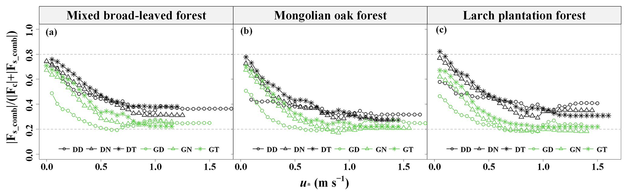
Figure 12Relative contribution ratio of the CO2 storage flux magnitude () determined by the decision-level fusion model as a function of the friction velocity (u∗) moving-block averages from all 30 min data for the years 2020–2021. GD represents the growing season's daytime, GN represents the growing season's nighttime, GT represents the growing season's transition period, DD represents the dormant season's daytime, DN represents the dormant season's nighttime, and DT represents the dormant season's transition period.
Table 3Linear regression coefficients of the relative contribution ratio of Fs_comb magnitudes to NEE observations () – driving-factor relationships for the six time periods.
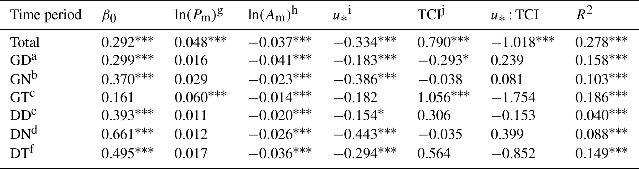
a GD represents the growing season's daytime. b GN represents the growing season's nighttime. c GT represents the growing season's transition period. d DD represents the dormant season's daytime. e DN represents the dormant season's nighttime. f DT represents the dormant season's transition period. g Pm represents the corresponding period of maximum amplitude. h Am represents maximum amplitude. i u∗ represents friction velocity. j TCI denotes the terrain complexity index.
P < 0.001. P < 0.01. ∗ P < 0.05.
As indicated in Table 3, both Pm and the TCI exhibited a significant positive correlation with (P < 0.05), while both Am and u∗ showed a significant negative correlation with (P < 0.05). Notably, seasonal variations in correlation coefficients were observed. The correlation between u∗ and was more pronounced during both the dormant season's transition period and the growing season, and it decreased with increasing TCI values during the dormant season's daytime and nighttime.
To evaluate the impact of Fs_comb on NEEobs (Fc+Fs), we further evaluated the slope (with intercept terms forced to zero) and NRMSE of Fc+Fs_comb compared to Fc+Fs_28, as presented in Tables S7 and S8. Fs_28 in the three forest stands was underestimated by 28.6 %–33.3 % compared to Fs_comb, and the NRMSE of Fs_comb versus Fs_28 ranged from 59.2 % to 67.2 %. NEEobs with Fs_28 was underestimated by 1.9 %–4.3 % compared to NEEobs with Fs_comb. The NRMSE of NEEobs with Fs_comb versus Fs_28 in the three forest stands ranged from 16.0 % to 25.4 %. The analysis suggested that combining the Fs values based on different averaging [CO2] time windows in the decision-level fusion model could successfully weight potential underestimation bias and random uncertainties.
The influences of Fs on the relationship between NEE observations and meteorological drivers indicated the effect of uncertainty in Fs estimates on NEE observations. Our analysis showed that the correlations between NEE observations derived from Fc+Fs and both photosynthetic photon flux density (PPFD) and air temperature are lower compared to those obtained from Fc alone (Figs. S1 and S2 in the Supplement). Additionally, the estimated light-saturated net CO2 assimilation (Amax) is greater when NEE observations are estimated by Fs+Fc, as opposed to when the NEE is estimated solely by Fc. This suggests that Fs significantly affects the daytime NEE and can correct the estimation of Amax and related parameters. The relationship between NEE observations and PPFD is influenced by the size of the averaging time window the Fs measurement. A larger averaging window results in less random uncertainty in the Fs estimation, thereby increasing the correlation between NEE observations and meteorological drivers, including PPFD and Ta.
4.1 Short-term [CO2] fluctuations above the forest canopy and Fs estimates in complex terrain
Compared to flat and uniform underlying surfaces, complex terrain and heterogeneous canopies modify the trajectory, speed distribution, and direction of the airflow. Increased wind speeds and shifting wind directions also increase turbulent activity above the canopy, facilitating the mixing and dispersion of CO2. This study found that short-term fluctuations in [CO2] above the canopy exhibited a range of 1 to 10 min (Fig. 2). These fluctuations were characterized by an average Pm ranging from 2.313 to 2.784 min (Table 2). Our results are in line with previous research using wavelet analysis, which reported fluctuation periods of [CO2] within and above the forest canopy to be between 14 and 116 s (Cava et al., 2004). These previous observations of the canopy waves during periods of extreme atmospheric stability (when ) exhibited a dominant period of 1–2 min, which is consistent with our findings. The period of [CO2] fluctuations was found to be predominantly influenced by turbulent fluxes and the residence time of CO2 within the canopy. This indicated a potential correlation between Pm and the residence time of CO2 within the canopy. Fuentes et al. (2006) employed a Lagrangian model and calculated the residence time of air parcels released near the ground and in the canopy, finding values ranging from 3 to 10 min and from 1 to 10 min, respectively. Similarly, Edburg et al. (2011) used the standard deviation of [CO2] averages to determine the CO2 residence time at different locations, including at the ground, within the canopy, and in their gas mixtures, yielding values of 8.6, 3.6, and 5.6 min, respectively. The results of these simulation experiments are consistent with our study, further supporting the association between [CO2] fluctuations above the forest canopy and CO2 residence time.
Tree density and canopy structure also play a role in influencing the air parcel residence time; on flat terrain, the air parcel residence time correlates with u∗ (Gerken et al., 2017), and an increase in the vegetation leaf area leads to longer residence times when turbulence is not fully penetrative. During the growing season, forests in our study site exhibit a higher leaf area index and greater canopy densities than during the dormant season (Li et al., 2023), resulting in higher Pm values of short-term [CO2] fluctuations above the canopy (Fig. 3). Additionally, at night, stable atmospheric conditions lead to longer residence times due to suppressed turbulent mixing, resulting in relatively high nighttime Pm values compared to daytime and transition periods (Fig. 3).
Complex terrain introduces complex changes into airflow structures, including gravity-induced waves, drainage, and nonlinear waves induced by single gusts, leading to dramatic [CO2] fluctuations. These dynamics contribute to uncertainties in estimating Fs. At night, the difference between incoming and outgoing longwave radiation over the valley soil surface and vegetation canopy gives rise to radiative cooling. Subsequently, the air near the soil surface experiences a gravity-induced downslope acceleration, potentially causing katabatic flow. As inertia-driven upslope winds are halted by katabatic acceleration, a local shallow drainage flow is established, reaching a quasi-equilibrium state approximately 1.5 h after sunset (Nadeau et al., 2013). Under stable atmospheric conditions, even gentle slopes (around 1°) can generate strong gravity-driven waves (Belušić and Mahrt, 2012). Consequently, advection may complicate the interpretation of nighttime EC measurements at certain relatively gentle sites, but this complexity is not evident during daytime measurements (Leuning et al., 2008). Advection plays a role in depleting the CO2 accumulated within the canopy, resulting in lower Fs fluxes and establishing an inverse relationship between storage and advection (van Gorsel et al., 2011). The occurrence of larger Fs values for high Pm values suggests weaker advection compared to low Pm values (Fig. 4). In our study, we observed that the Fs magnitude was relatively large during nighttime and transition periods, while it was smaller during the daytime (Fig. 4), which is consistent with the findings reported by Wang et al. (2016).
The terrain unevenness and the complexity of canopy structure significantly affect the airflow divergence in the atmospheric boundary layer. This results in weakened air circulation within the canopy and spatial variation in the patterns and extent of airflow separation (Grant et al., 2015). During nighttime and transition periods in a closed canopy, the turbulent coupling state above and below the canopy gradually decouples, eventually reaching complete decoupling as u∗ decreases (Fig. 5). However, this decoupling does not lead to stable stratification within the canopy. Despite the occurrence of decoupling and advection in the closed canopy, waves are unlikely to exist within the canopy itself (van Gorsel et al., 2011). As a result, a consistent trend in the variation in Fs with τ is observed across the three forest stands during the growing season, independent of Pm (Fig. 9). Conversely, in an open canopy where waves are present, the observations of Fs become more complex. This complexity could be the primary reason for the variation in Fs with [CO2] averaging time windows differing between the three forest stands for low Pm values during the dormant-season daytime (Fig. 9). The presence of waves introduces additional variability into the measurements, leading to differences in Fs estimates based on different [CO2] averaging time windows in these particular conditions.
4.2 Uncertainty in forest ecosystem Fs measurement in complex terrain
The random uncertainty in Fs shares similarities with NEE estimation. For example, the magnitude of Fs measurements is positively correlated with the standard deviation of random uncertainty in Fs. Additionally, the overall distribution of Fs measurements exhibits a non-Gaussian distribution with a high peak, aligning with the statistical properties of NEE uncertainty (Richardson et al., 2006, 2008). The uncertainty in the storage term depends a great deal on the setup used, together with the biological activity of the ecosystem and the height of the control volume. In addition, various factors contribute to the uncertainty in Fs estimates, including the flux measurement footprint variations, sampling frequency, the spatial sampling resolution of CO2 and H2O concentrations, and instrumental measurement accuracy. The accuracy and precision requested for the CO2 and H2O concentration measurements are ±1 µmol mol−1 and ±1 mmol mol−1, respectively (Montagnani et al., 2018). The uncertainty arising from variations in the flux measurement footprint is considerable, typically on the order of tens of percent, which is an order of magnitude higher than typical sensor errors (Metzger, 2018). AP200 adopts buffer volumes to mix the gas. The LI-850 analyzer integrated within AP200 exhibits a sensitivity to water vapor of less than 0.1 µmol CO2 per mmol mol−1 H2O and a sensitivity to CO2 of less than 0.0001 mmol mol−1 H2O per µmol CO2. Efforts to reduce random errors in [CO2] originating from pressure fluctuations include adding buffer volumes before IRGA pumping tests (Marcolla et al., 2014). The buffer volumes are fully mixed during gas extraction, and a weighted average of [CO2] instantaneous measurements is obtained to minimize the sampling error for each level's [CO2] measurement (Cescatti et al., 2016).
The Fs estimates can be influenced by singular eddies that penetrate the canopy (Finnigan, 2006). Accurate calculation of Fs requires considering the period of [CO2] fluctuations with the eddy coherence structure. The spectral energy of the Fs time series is primarily concentrated between 0.001 and 0.2 Hz (500 and 5 s, respectively). However, even with sampling frequencies of 2 Hz and below, significantly lower Fs values are obtained (Bjorkegren et al., 2015). The Nyquist–Shannon sampling theorem dictates that accurate measurements of [CO2] require a sampling period that is no longer than half the period of [CO2] fluctuations. Consequently, to monitor short-term changes in [CO2], measurements must be taken over a period that is no longer than half of the period corresponding to the maximum amplitude (or major energy) of [CO2] fluctuations. In this study, the average Pm for [CO2] fluctuations fell within the range of 2.313–2.784 min (Table 2). Therefore, it is crucial to ensure that the sampling period for [CO2] does not exceed 1.256 to 1.392 min, which corresponds to half the average Pm range. Monitoring fluctuations in Pm for less than 4 min during a 2 min monitoring period of [CO2] presents a significant challenge. This is a primary reason for the systematic bias and random error in the Fs estimate with a single-profile system being irreconcilable (Wang et al., 2016). Short-term [CO2] fluctuations are mainly influenced by boundary-layer turbulence, and sampling errors in incomplete fluctuation cycles are superimposed with the real advection flux (anisotropy) dispersion in complex terrain (van Gorsel et al., 2011). This substantially increases the random uncertainty in Fs based on shorter [CO2] averaging time windows (Figs. 6 and 8). As a result, the deviation of NEE estimates from the actual value expands.
Fluxes in heterogeneous regions are significantly higher than in uniform regions. The energy transfer from the ground surface to large eddies occurs primarily in areas with pronounced heterogeneity, and this energy distribution is uneven across the region (Aubinet et al., 2012). Once large-scale eddies acquire energy, their cascading of energy to smaller-scale eddies is influenced by topographic features, leading to variations in these smaller-scale eddies along different flow streams (Chen et al., 2023). In complex terrain, the bidirectional airflow within forests along slopes can cause the decoupling of soil CO2 fluxes from EC measurements above the forest canopy (Feigenwinter et al., 2008; Aubinet et al., 2003), leading to significant errors in CO2 flux measurements. Forest soil serves as the primary source of CO2 gas, and regions of high flux over complex terrain act like chimneys, transporting air parcels from the soil surface within forests (Chen et al., 2019). By increasing the number of gas concentration sampling points near the ground, the horizontal representativeness can be enhanced, thereby reducing the bias in the estimation of Fs (Nicolini et al., 2018). In situations where turbulence is not well developed and CO2 mixing is inadequate, the trend of Fs with turbulence intensity aligns with that of advective fluxes, which is the opposite to that of turbulent fluxes (McHugh et al., 2017). The temporal dynamics and amplitudes of Fs changes are influenced by topography complexity and wind conditions above the forest canopy (Fig. 10). Locations with more complex and sloping topography at the flux tower are more likely to generate advective fluxes that may not be easily observed at a single point.
Estimating landscape CO2 fluxes in complex terrain solely based on measurements from a single flux tower can introduce significant errors and biases that are not acceptable. The magnitude of these errors in Fs estimates is dependent on the height of the forest canopy and the endogenous source/sink (Chen et al., 2020). To mitigate errors and biases associated with estimating Fs in complex terrain, we employed a regression modeling approach using the decision-level fusion model. This method involves computing a weighted average of Fs based on different [CO2] averaging time windows, effectively reducing errors and biases in the estimation of Fs (see Table 5). In fact, from the definition of storage flux, it can be seen that weighting the storage flux essentially means weighting the [CO2] in the averaging time window, which in turn means replacing spatial sequences with temporal sequences for weighting. The weighting coefficients used to construct the model were based on the relative errors and biases in Fs estimation, with the weighting coefficient decreasing as the represented moment's length increased. To obtain more accurate estimates of forest ecosystem Fs in complex terrain, further research should focus on understanding the spatiotemporal patterns and dynamics of [CO2].
This study investigated the impact of short-term [CO2] fluctuations on the estimation of Fs in temperate forest ecosystems within complex terrain. Additionally, it examined the Fs uncertainty and the contribution of Fs to the NEE using data from three flux towers. To enhance Fs uncertainty estimation, statistical sampling techniques were applied based on an individual-tower approach.
The results highlighted the significance of considering multiple time windows for averaging [CO2] when estimating Fs, as [CO2] above the forest canopies exhibited fluctuations with periods ranging from 1 to 10 min. Diurnal, seasonal, and spatial variations were observed in the amplitude and periodicity of [CO2] fluctuations, highlighting the need for thoughtful sampling strategies. The use of individual gas analyzers to sample the CO2 in the control volume was inadequate, leading to systematic biases and random errors in the Fs estimates. Increasing [CO2] averaging time windows mitigated the effect of [CO2] fluctuations on Fs estimates, reducing both their magnitude and their uncertainty.
The study also revealed that the uncertainty in Fs followed a non-normal distribution, with its standard deviation positively correlated with Fs magnitude, which has important implications for quality control. To improve Fs estimation, a decision-level fusion model was introduced, integrating Fs estimates from multiple [CO2] averaging time windows, effectively reducing the impact of short-term [CO2] fluctuations while considering underestimation bias and random errors. The contribution of Fs to the NEE exhibited diurnal, seasonal, and spatial variations associated with u∗, contributing to the NEE observations at rates ranging from 17.2 % to 82.0 % depending on the turbulent mixing and terrain complexity. The influence of terrain complexity on the relationship between [CO2] fluctuations, turbulent mixing, and the contribution of Fs to the NEE was also evident. The findings from the three flux towers allowed for the generalization of these results beyond the study site. These insights provide crucial scientific support for the practical application of the eddy covariance technique and advance our understanding of accurately estimating the NEE in forest ecosystems in complex terrain.
A1 The weight parameters of the decision-level fusion model
For each 30 min CO2 storage flux (Fs) estimate based on the CO2 concentration ([CO2]) averaging time window (τ), the weight in the decision-level fusion model can be obtained by weighting the random uncertainty and bias in Fs_τ.
The weight of the random uncertainty for Fs_τ is expressed as follows:
where σ(ετ) is the random uncertainty in Fs_τ, qualified as the standard deviation.
The weight of the bias for Fs_τ is expressed as follows:
where Kτ is the slope between Fs_τ and Fs_28.
Ultimately, the weight of Fs_τ in the decision-level fusion model can be calculated using the following equation:
where r represents the proportion of the weight of random uncertainty.
A2 Complex-terrain index
This study employed a novel descriptor called the terrain complexity index (TCI) to quantify the complexity of the three-dimensional terrain. For a given unit area, the TCI equation can be expressed as follows:
where Pd represents the volume of terrain above the lowest elevation of an area unit (Vu) divided by the product of its largest vertically projected area (Sv) and the edge length of the side of the area unit (d), expressed as ; Pd is defined as 1 when Sv is 0. Given Vu, an increase in Sv correlates with a higher degree of terrain complexity. Notably, Pd is defined as 1 when the terrain volume is 0 or when the terrain surface of the area unit is parallel to the horizontal plane and is smooth and homogeneous. αd indicates the slope of the area unit. Zd denotes the terrain roughness, which is defined as the ratio of the terrain surface area to the projected horizontal plane (Loke and Chisholm, 2022). The value of Zd was in the range of [1, +∞). The larger the Zd, the more complex the terrain. Df is the fractal dimension of the terrain surface area, which ranged from 2 to 3 and describes the complexity in the spatially self-similar structure of the local surface within the area unit and the area unit surface (Mandelbrot, 1967; Taud and Parrot, 2005). Employing the terrain surface area, the box-counting method was used to estimate the fractal dimension of the unit area. H represents the Shannon–Wiener index and is expressed as , capturing the uniformity of the spatial distribution of the pixel aspects within the area unit (Brown, 1997). When the aspect of each pixel is divided into 30° segments, Pi denotes the proportion of the ith type of pixel aspects within the area unit and n is the total number of pixel aspect types within the area unit. A larger H indicates a more complex terrain. When the number of pixel aspect types in the area unit is kept constant, it is essential to recognize that greater uniformity in the distribution of all pixel aspects in the area unit results in a larger H. Similarly, when the uniformity of the distribution of pixel aspects in the area unit is kept constant, a larger H is achieved with an increase in the observation of the number of pixel aspect types.
To quantify the terrain complexity of the underlying surface around the flux towers, we computed the quartiles of the TCI for all area units within a sector (divided by 30°) with a radius of 380 m. A weighted geometric mean was employed to construct TCIs, which describes the statistical distribution of the TCI of the sector. TCIs represents the topographic complexity of the sector and is calculated using the following equation:
where TCI5, TCI25, TCI50, TCI75, and TCI95 are the quartiles of 5 %, 25 %, 50 %, 75 %, and 95 %, respectively. The TCIs values range from 0 to 1, with higher values indicating greater terrain complexity.
Data used in this paper are available at the Science Data Bank (https://www.scidb.cn/en/s/7ZfQZv, Teng et al., 2023) or upon request to the corresponding author.
The supplement related to this article is available online at: https://doi.org/10.5194/amt-17-5581-2024-supplement.
DT developed the manuscript; JZ was responsible for conceptualizing the idea and designing the research study; TG substantially structured the manuscript; FY contributed to the data collection process; YZ helped in the design and preparation of the figures and tables; XZ and BY revised the manuscript.
The contact author has declared that none of the authors has any competing interests.
Publisher’s note: Copernicus Publications remains neutral with regard to jurisdictional claims made in the text, published maps, institutional affiliations, or any other geographical representation in this paper. While Copernicus Publications makes every effort to include appropriate place names, the final responsibility lies with the authors.
We are grateful to Qingyuan Forest CERN, Chinese Academy of Sciences–Qingyuan Forest, National Observation and Research Station, Liaoning Province, China, for providing forest sites, instrument systems, and logistical support.
This research was financially supported by the National Natural Science Foundation of China (grant no. 32192435), the China Postdoctoral Science Foundation (grant no. 2023M733672), the Key R&D Program of Liaoning Province (2023JH2/101800043), and the Postdoctoral Research Startup Foundation of Liaoning Province of China (grant no. 2022-BS-022).
This paper was edited by Luca Mortarini and reviewed by Leonardo Montagnani and Ivan Mauricio Cely Toro.
Aubinet, M., Grelle, A., Ibrom, A., Rannik, Ü., Moncrieff, J., Foken, T., Kowalski, A. S., Martin, P. H., Berbigier, P., Bernhofer, C., Clement, R., Elbers, J., Granier, A., Grünwald, T., Morgenstern, K., Pilegaard, K., Rebmann, C., Snijders, W., Valentini, R., and Vesala, T.: Estimates of the Annual Net Carbon and Water Exchange of Forests: The EUROFLUX Methodology, Adv. Ecol. Res., 30, 113–175, https://doi.org/10.1016/s0065-2504(08)60018-5, 2000.
Aubinet, M., Heinesch, B., and Yernaux, M.: Horizontal and Vertical CO2 Advection In A Sloping Forest, Bound.-Lay. Meteorol., 108, 397–417, https://doi.org/10.1023/a:1024168428135, 2003.
Aubinet, M., Vesala, T., and Papale, D.: Eddy Covariance: A Practical Guide to Measurement and Data Analysis, Springer Atmospheric Sciences, Springer, Dordrecht, XXII, 438 pp., https://doi.org/10.1007/978-94-007-2351-1, 2012.
Belušić, D. and Mahrt, L.: Is geometry more universal than physics in atmospheric boundary layer flow?, J. Geophys. Res.-Atmos., 117, D09115, https://doi.org/10.1029/2011jd016987, 2012.
Bjorkegren, A. B., Grimmond, C. S. B., Kotthaus, S., and Malamud, B. D.: CO2 emission estimation in the urban environment: Measurement of the CO2 storage term, Atmos. Environ., 122, 775–790, https://doi.org/10.1016/j.atmosenv.2015.10.012, 2015.
Brown, S.: Estimating Biomass and Biomass Change of Tropical Forests: A Primer, FAO Forestry Paper, 37–39, 1997.
Cava, D., Giostra, U., Siqueira, M., and Katul, G.: Organised motion and radiative perturbations in the nocturnal canopy sublayer above an even-aged pine forest, Bound.-Lay. Meteorol., 112, 129–157, https://doi.org/10.1023/B:BOUN.0000020160.28184.a0, 2004.
Cescatti, A., Marcolla, B., Goded, I., and Gruening, C.: Optimal use of buffer volumes for the measurement of atmospheric gas concentration in multi-point systems, Atmos. Meas. Tech., 9, 4665–4672, https://doi.org/10.5194/amt-9-4665-2016, 2016.
Chen, B., Chamecki, M., and Katul, G. G.: Effects of topography on in-canopy transport of gases emitted within dense forests, Q. J. Roy. Meteor. Soc., 145, 2101–2114, https://doi.org/10.1002/qj.3546, 2019.
Chen, B. C., Chamecki, M., and Katul, G. G.: Effects of Gentle Topography on Forest-Atmosphere Gas Exchanges and Implications for Eddy-Covariance Measurements, J. Geophys. Res.-Atmos., 125, e2020JD032581, https://doi.org/10.1029/2020JD032581, 2020.
Chen, J., Chen, X., Jia, W., Yu, Y., and Zhao, S.: Multi-sites observation of large-scale eddy in surface layer of Loess Plateau, Sci. China Earth Sci., 66, 871–881, https://doi.org/10.1007/s11430-022-1035-4, 2023.
de Araújo, A. C., Ometto, J. P. H. B., Dolman, A. J., Kruijt, B., Waterloo, M. J., and Ehleringer, J. R.: Implications of CO2 pooling on δ13C of ecosystem respiration and leaves in Amazonian forest, Biogeosciences, 5, 779–795, https://doi.org/10.5194/bg-5-779-2008, 2008.
de Araújo, A. C., Dolman, A. J., Waterloo, M. J., Gash, J. H. C., Kruijt, B., Zanchi, F. B., de Lange, J. M. E., Stoevelaar, R., Manzi, A. O., Nobre, A. D., Lootens, R. N., and Backer, J.: The spatial variability of CO2 storage and the interpretation of eddy covariance fluxes in central Amazonia, Agr. Forest Meteorol., 150, 226–237, https://doi.org/10.1016/j.agrformet.2009.11.005, 2010.
Edburg, S. L., Stock, D., Lamb, B. K., and Patton, E. G.: The Effect of the Vertical Source Distribution on Scalar Statistics within and above a Forest Canopy, Bound.-Lay. Meteorol., 142, 365–382, https://doi.org/10.1007/s10546-011-9686-1, 2011.
Feigenwinter, C., Bernhofer, C., and Vogt, R.: The Influence of Advection on the Short Term CO2-Budget in and Above a Forest Canopy, Bound.-Lay. Meteorol., 113, 201–224, https://doi.org/10.1023/B:BOUN.0000039372.86053.ff, 2004.
Feigenwinter, C., Bernhofer, C., Eichelmann, U., Heinesch, B., Hertel, M., Janous, D., Kolle, O., Lagergren, F., Lindroth, A., Minerbi, S., Moderow, U., Mölder, M., Montagnani, L., Queck, R., Rebmann, C., Vestin, P., Yernaux, M., Zeri, M., Ziegler, W., and Aubinet, M.: Comparison of horizontal and vertical advective CO2 fluxes at three forest sites, Agr. Forest Meteorol., 148, 12–24, https://doi.org/10.1016/j.agrformet.2007.08.013, 2008.
Finnigan, J.: The storage term in eddy flux calculations, Agr. Forest Meteorol., 136, 108–113, https://doi.org/10.1016/j.agrformet.2004.12.010, 2006.
Finnigan, J., Ayotte, K., Harman, I., Katul, G., Oldroyd, H., Patton, E., Poggi, D., Ross, A., and Taylor, P.: Boundary-Layer Flow Over Complex Topography, Bound.-Lay. Meteorol., 177, 247–313, https://doi.org/10.1007/s10546-020-00564-3, 2020.
Fuentes, J. D., Wang, D., Bowling, D. R., Potosnak, M., Monson, R. K., Goliff, W. S., and Stockwell, W. R.: Biogenic Hydrocarbon Chemistry within and Above a Mixed Deciduous Forest, J. Atmos. Chem., 56, 165–185, https://doi.org/10.1007/s10874-006-9048-4, 2006.
Gao, T., Yu, L.-Z., Yu, F.-Y., Wang, X.-C., Yang, K., Lu, D.-L., Li, X.-F., Yan, Q.-L., Sun, Y.-R., Liu, L.-F., Xu, S., Zhen, X.-J., Ni, Z.-D., Zhang, J.-X., Wang, G.-F., Wei, X.-H., Zhou, X.-H., and Zhu, J.-J.: Functions and applications of Multi-Tower Platform of Qingyuan Forest Ecosystem Research Station of Chinese Academy of Sciences, Chinese Journal of Applied Ecology, 31, 695–705, https://doi.org/10.13287/j.1001-9332.202003.040, 2020.
Gerken, T., Chamecki, M., and Fuentes, J. D.: Air-Parcel Residence Times Within Forest Canopies, Bound.-Lay. Meteorol., 165, 29–54, https://doi.org/10.1007/s10546-017-0269-7, 2017.
Grant, E. R., Ross, A. N., Gardiner, B. A., and Mobbs, S. D.: Field Observations of Canopy Flows over Complex Terrain, Bound.-Lay. Meteorol., 156, 231–251, https://doi.org/10.1007/s10546-015-0015-y, 2015.
Gu, L., Massman, W. J., Leuning, R., Pallardy, S. G., Meyers, T., Hanson, P. J., Riggs, J. S., Hosman, K. P., and Yang, B.: The fundamental equation of eddy covariance and its application in flux measurements, Agr. Forest Meteorol., 152, 135–148, https://doi.org/10.1016/j.agrformet.2011.09.014, 2012.
Heinesch, B., Yernaux, M., and Aubinet, M.: Some methodological questions concerning advection measurements: a case study, Bound.-Lay. Meteorol., 122, 457–478, https://doi.org/10.1007/s10546-006-9102-4, 2007.
Hollinger, D. Y. and Richardson, A. D.: Uncertainty in eddy covariance measurements and its application to physiological models, Tree Physiol., 25, 873–885, https://doi.org/10.1093/treephys/25.7.873, 2005.
Huang, N. E. and Wu, Z.: A review on Hilbert-Huang transform: Method and its applications to geophysical studies, Rev. Geophys., 46, RG2006, https://doi.org/10.1029/2007rg000228, 2008.
Huang, N. E., Shen, Z., Long, S. R., Wu, M. C., Shih, H. H., Zheng, Q., Yen, N.-C., Tung, C. C., and Liu, H. H.: The empirical mode decomposition and the Hilbert spectrum for nonlinear and non-stationary time series analysis, P. Roy. Soc. Lond. A, 454, 903–995, https://doi.org/10.1098/rspa.1998.0193, 1998.
Khélifa, N., Lecollinet, M., and Himbert, M.: Molar mass of dry air in mass metrology, Measurement, 40, 779–784, https://doi.org/10.1016/j.measurement.2006.05.009, 2007.
Leuning, R., Zegelin, S. J., Jones, K., Keith, H., and Hughes, D.: Measurement of horizontal and vertical advection of CO2 within a forest canopy, Agr. Forest Meteorol., 148, 1777–1797, https://doi.org/10.1016/j.agrformet.2008.06.006, 2008.
Li, S., Yan, Q., Liu, Z., Wang, X., Yu, F., Teng, D., Sun, Y., Lu, D., Zhang, J., Gao, T., and Zhu, J.: Seasonality of albedo and fraction of absorbed photosynthetically active radiation in the temperate secondary forest ecosystem: A comprehensive observation using Qingyuan Ker towers, Agr. Forest Meteorol., 333, 109418, https://doi.org/10.1016/j.agrformet.2023.109418, 2023.
Li, Y.-C., Liu, F., Wang, C.-K., Gao, T., and Wang, X.-C.: Carbon budget estimation based on different methods of CO2 storage flux in forest ecosystems, Chinese Journal of Applied Ecology, 31, 3665–3673, https://doi.org/10.13287/j.1001-9332.202011.004, 2020.
Loke, L. H. L. and Chisholm, R. A.: Measuring habitat complexity and spatial heterogeneity in ecology, Ecol. Lett., 25, 2269–2288, https://doi.org/10.1111/ele.14084, 2022.
Mandelbrot, B. B.: How Long Is the Coast of Britain? Statistical Self-Similarity and Fractional Dimension, Science, 156, 636–638, 1967.
Marcolla, B., Cobbe, I., Minerbi, S., Montagnani, L., and Cescatti, A.: Methods and uncertainties in the experimental assessment of horizontal advection, Agr. Forest Meteorol., 198–199, 62–71, https://doi.org/10.1016/j.agrformet.2014.08.002, 2014.
McHugh, I. D., Beringer, J., Cunningham, S. C., Baker, P. J., Cavagnaro, T. R., Mac Nally, R., and Thompson, R. M.: Interactions between nocturnal turbulent flux, storage and advection at an “ideal” eucalypt woodland site, Biogeosciences, 14, 3027–3050, https://doi.org/10.5194/bg-14-3027-2017, 2017.
McMaster, G. S. and Wilhelm, W. W.: Growing degree-days: one equation, two interpretations, Agr. Forest Meteorol., 87, 291–300, https://doi.org/10.1016/S0168-1923(97)00027-0, 1997.
Metzger, S.: Surface-atmosphere exchange in a box: Making the control volume a suitable representation for in-situ observations, Agr. Forest Meteorol., 255, 68–80, https://doi.org/10.1016/j.agrformet.2017.08.037, 2018.
Montagnani, L., Manca, G., Canepa, E., Georgieva, E., Acosta, M., Feigenwinter, C., Janous, D., Kerschbaumer, G., Lindroth, A., Minach, L., Minerbi, S., Mölder, M., Pavelka, M., Seufert, G., Zeri, M., and Ziegler, W.: A new mass conservation approach to the study of CO2 advection in an alpine forest, J. Geophys. Res., 114, D07306, https://doi.org/10.1029/2008jd010650, 2009.
Montagnani, L., Grunwald, T., Kowalski, A., Mammarella, I., Merbold, L., Metzger, S., Sedlak, P., and Siebicke, L.: Estimating the storage term in eddy covariance measurements: the ICOS methodology, Int. Agrophys., 32, 551–567, https://doi.org/10.1515/intag-2017-0037, 2018.
Nadeau, D. F., Pardyjak, E. R., Higgins, C. W., Huwald, H., and Parlange, M. B.: Flow during the evening transition over steep Alpine slopes, Q. J. Roy. Meteor. Soc., 139, 607–624, https://doi.org/10.1002/qj.1985, 2013.
Nicolini, G., Aubinet, M., Feigenwinter, C., Heinesch, B., Lindroth, A., Mamadou, O., Moderow, U., Mölder, M., Montagnani, L., Rebmann, C., and Papale, D.: Impact of CO2 storage flux sampling uncertainty on net ecosystem exchange measured by eddy covariance, Agr. Forest Meteorol., 248, 228–239, https://doi.org/10.1016/j.agrformet.2017.09.025, 2018.
Richardson, A. D., Hollinger, D. Y., Burba, G. G., Davis, K. J., Flanagan, L. B., Katul, G. G., William Munger, J., Ricciuto, D. M., Stoy, P. C., Suyker, A. E., Verma, S. B., and Wofsy, S. C.: A multi-site analysis of random error in tower-based measurements of carbon and energy fluxes, Agr. Forest Meteorol., 136, 1–18, https://doi.org/10.1016/j.agrformet.2006.01.007, 2006.
Richardson, A. D., Mahecha, M. D., Falge, E., Kattge, J., Moffat, A. M., Papale, D., Reichstein, M., Stauch, V. J., Braswell, B. H., Churkina, G., Kruijt, B., and Hollinger, D. Y.: Statistical properties of random CO2 flux measurement uncertainty inferred from model residuals, Agr. Forest Meteorol., 148, 38–50, https://doi.org/10.1016/j.agrformet.2007.09.001, 2008.
Sha, J., Zou, J., and Sun, J.: Observational study of land-atmosphere turbulent flux exchange over complex underlying surfaces in urban and suburban areas, Sci. China Earth Sci., 64, 1050–1064, https://doi.org/10.1007/s11430-020-9783-2, 2021.
Siebicke, L., Steinfeld, G., and Foken, T.: CO2-gradient measurements using a parallel multi-analyzer setup, Atmos. Meas. Tech., 4, 409–423, https://doi.org/10.5194/amt-4-409-2011, 2011.
Taud, H. and Parrot, J.-F.: Measurement of DEM roughness using the local fractal dimension, Géomorphologie, 11, 327–338, https://doi.org/10.4000/geomorphologie.622, 2005.
Teng, D., Zhu, J., Gao, T., and Yu, F.: High-Frequency Eddy Covariance Measurements of CO2 Fluxes in a Mountain Watershed: A Comprehensive Dataset for Understanding Carbon Exchange Dynamics in Forest Ecosystems[DS/OL], V1, Science Data Bank [data set], https://www.scidb.cn/en/s/7ZfQZv (last access: 18 September 2024), 2023.
van Gorsel, E., Harman, I. N., Finnigan, J. J., and Leuning, R.: Decoupling of air flow above and in plant canopies and gravity waves affect micrometeorological estimates of net scalar exchange, Agr. Forest Meteorol., 151, 927–933, https://doi.org/10.1016/j.agrformet.2011.02.012, 2011.
Wang, J., Shi, T., Yu, D., Teng, D., Ge, X., Zhang, Z., Yang, X., Wang, H., and Wu, G.: Ensemble machine-learning-based framework for estimating total nitrogen concentration in water using drone-borne hyperspectral imagery of emergent plants: A case study in an arid oasis, NW China, Environ. Pollut., 266, 115412, https://doi.org/10.1016/j.envpol.2020.115412, 2020.
Wang, X., Wang, C., Guo, Q., and Wang, J.: Improving the CO2 storage measurements with a single profile system in a tall-dense-canopy temperate forest, Agr. Forest Meteorol., 228–229, 327–338, https://doi.org/10.1016/j.agrformet.2016.07.020, 2016.
Warton, D. I., Duursma, R. A., Falster, D. S., and Taskinen, S.: smatr 3 – an R package for estimation and inference about allometric lines, Methods Ecol. Evol., 3, 257–259, https://doi.org/10.1111/j.2041-210X.2011.00153.x, 2012.
Webb, E. K., Pearman, G. I., and Leuning, R.: Correction of flux measurements for density effects due to heat and water vapour transfer, Q. J. Roy. Meteor. Soc., 106, 85–100, https://doi.org/10.1002/qj.49710644707, 1980.
Xu, K., Pingintha-Durden, N., Luo, H., Durden, D., Sturtevant, C., Desai, A. R., Florian, C., and Metzger, S.: The eddy-covariance storage term in air: Consistent community resources improve flux measurement reliability, Agr. Forest Meteorol., 279, 107734, https://doi.org/10.1016/j.agrformet.2019.107734, 2019.
Yang, B., Hanson, P. J., Riggs, J. S., Pallardy, S. G., Heuer, M., Hosman, K. P., Meyers, T. P., Wullschleger, S. D., and Gu, L.-H.: Biases of CO2 storage in eddy flux measurements in a forest pertinent to vertical configurations of a profile system and CO2 density averaging, J. Geophys. Res., 112, D20123, https://doi.org/10.1029/2006jd008243, 2007.
Yang, P. C., Black, T. A., Neumann, H. H., Novak, M. D., and Blanken, P. D.: Spatial and temporal variability of CO2 concentration and flux in a boreal aspen forest, J. Geophys. Res.-Atmos., 104, 27653–27661, https://doi.org/10.1029/1999jd900295, 1999.
Yao, Y., Zhang, Y., Yu, G., Song, Q., Tan, Z., and Zhao, J.: Estimation of CO2 storage flux between forest and atmosphere in a tropical forest, Journal of Beijing Forestry University, 33, 23–29, 2011.
Zhang, M., Wen, X., Yu, G.-R., Zhang, L.-M., Fu, Y., Sun, X., and Han, S.-J.: Effects of CO2 storage flux on carbon budget of forest ecosystem, Chinese Journal of Applied Ecology, 21, 1201–1209, 2010.
Zhu, J., Gao, T., Yu, L., Yu, F., Yang, K., Lu, D., Yan, Q., Sun, Y., Liu, L., Xu, S., Zhang, J., Zheng, X., Song, L., and Zhou, X.: Functions and Applications of Multi-tower Platform of Qingyuan Forest Ecosystem Research Station of Chinese Academy of Sciences (Qingyuan Ker Towers), Bulletin of the Chinese Academy of Sciences, 36, 351–361, https://doi.org/10.16418/j.issn.1000-3045.20210304002, 2021.