the Creative Commons Attribution 4.0 License.
the Creative Commons Attribution 4.0 License.
 | 26 Sep 2024
Retrieval of pseudo-BRDF-adjusted surface reflectance at 440 nm from the Geostationary Environmental Monitoring Spectrometer (GEMS)
Suyoung Sim
Sungwon Choi
Daeseong Jung
Jongho Woo
Nayeon Kim
Sungwoo Park
Honghee Kim
Ukkyo Jeong
Hyunkee Hong
In satellite remote sensing applications, enhancing the precision of level 2 (L2) algorithms relies heavily on the accurate estimation of the surface reflectance across the ultraviolet (UV) to visible (VIS) spectrum. However, the mutual dependence between the L2 algorithms and the surface reflectance retrieval poses challenges, necessitating an alternative approach. To address this issue, many satellite algorithms generate Lambertian-equivalent reflectivity (LER) products as a priori surface reflectance data; however, this often results in an underestimation of these data. This study is the first to assess the applicability of background surface reflectance (BSR), derived using a semi-empirical bidirectional reflectance distribution function (BRDF) model, in an operational environmental satellite algorithm. This study pioneered the application of the BRDF model to hyperspectral satellite data at 440 nm, aiming to provide more realistic preliminary surface reflectance data. In this study, the Geostationary Environment Monitoring Spectrometer (GEMS) data were used, and a comparative analysis of the GEMS BSR and GEMS LER retrieved in this study revealed an improvement in the relative root mean squared error (rRMSE) accuracy of 3 %. Additionally, a time series analysis across diverse land types indicated a greater stability exhibited by the BSR than by the LER. For further validation, the BSR was compared with other LER databases using ground-truth data, yielding superior simulation performance. These findings present a promising avenue for enhancing the accuracy of surface reflectance retrieval from hyperspectral satellite data, thereby advancing the practical applications of satellite remote sensing algorithms.
- Article
(5881 KB) - Full-text XML
- BibTeX
- EndNote


Surface reflectance, the fraction of solar radiation reflected by the Earth's surface, is a key parameter in meteorology, environmental studies, and climate research (Dickinson, 1983). Because surface reflectance is utilized in remote sensing systems to derive various geophysical, chemical, and biological variables (Veefkind et al., 2006; Noguchi et al., 2014), accurate satellite observations of land surface reflectance are essential for developing accurate satellite remote sensing algorithms. Ultraviolet (UV) to visible (VIS) surface reflectance is of great importance for atmospheric component retrieval algorithms and related studies, especially as an input to various level 2 (L2) algorithms, including aerosols, clouds, ozone, and gas tracers (Lin et al., 2015; Lorente et al., 2018).
However, it is difficult to determine the calculation precedence between these L2 algorithms and the surface reflection algorithms. Surface reflectance is the fundamental input data for other L2 algorithms, and L2 data are also essential for surface reflectance retrieval algorithms. In the retrieval of surface reflectance, aerosol optical depth (AOD) and atmospheric gas products (such as ozone, total precipitable water (TPW), and nitrogen dioxide (NO2)) are fundamental parameters. Simultaneously, surface reflectance is crucial for the retrieval of these atmospheric constituents and forms an essential component of their product. This reciprocal relationship has a significant effect on the accuracy of the calculated data. Therefore, a background field for AOD and atmospheric products should be established when calculating surface reflectance, or conversely, a background field for surface reflectance should be developed when calculating AOD and atmospheric substances. Therefore, several studies have calculated and applied alternative surface reflectance data to overcome this dilemma.
Most satellite algorithms that focus on observing the UV–VIS region, such as the Total Ozone Mapping Spectrometer (TOMS) (Herman and Celarier, 1997), Global Ozone Monitoring Experiment (GOME) (Koelemeijer et al., 2003), and Ozone Monitoring Instrument (OMI) (Kleipool et al., 2008), produce a priori surface reflectance products called Lambertian-equivalent reflectivity (LER). The LER archive is a climatology database calculated using the minimum reflectance method under the assumption of a Lambertian surface. The minimum reflectance technique uses the lowest observed ground reflectance for the same pixel within the compositing period. This technique assumes that the minimum value of the surface reflectance generated during the synthesis period minimizes the effects of the atmosphere and clouds and adopts it as a stable value in a clear sky. This method has the advantage of being simple to implement but has a limitation in that it cannot consider realistic surface reflection properties and can easily underestimate the actual surface reflectance. Occasionally, overcalculations can occur because of a failure to reflect the characteristics of changes in the indicators in real time. Therefore, to identify a more realistic surface signal, the GOME-2 (Tilstra et al., 2017) LER products have introduced the MODE-LER method alongside the MIN-LER approach. While the MIN-LER method selects the minimum reflectance observed during the synthesis period as well known, the MODE-LER method identifies the most frequently occurring reflectance value. This approach provides a more representative measure of typical surface reflectance, especially in regions with highly variable surface conditions. Although the MODE-LER method offers more improvements compared to the minimum reflectance method, it remains a climatological dataset and cannot fully parameterize the anisotropic reflectance properties of surfaces, which change in real time.
Underestimated and overestimated surface reflectance arising from neglecting surface anisotropy can significantly compromise the accuracy of other satellite-derived products such as AOD (Kaufman et al., 1997), formaldehyde (HCHO) (De Smedt et al., 2018; Howlett et al., 2023), and NO2 and SO2 (Leitão et al., 2010; McLinden et al., 2014). For instance, an underestimated surface reflectance may result in an overestimation of the AOD (Mei et al., 2014), affecting the accuracy of aerosol concentration estimate. Conversely, if the surface reflectance is overestimated, the opposite effects would occur (Chen et al., 2021; Wang et al., 2019). Li et al. (2012) found that a variation of 0.05 in the surface reflectance in the blue channel can lead to an underestimation of approximately −0.17 in the range where the AOD is less than 0.4. Veefkind et al. (2000) indicated that an error of 0.01 in the surface reflectance in the UV region results in an AOD error of 0.1. Furthermore, Platnick et al. (2001) and Letu et al. (2020) observed that errors in cloud retrieval can also occur, affecting cloud properties such as cloud fraction and optical thickness. According to Lorente et al. (2018), clear-sky air mass factors (AMFs) are up to 20 % higher and cloud radiance fractions are up to 40 % lower if surface anisotropic reflectance is considered. Furthermore, biases may arise in the estimation of trace gas concentrations, affecting the reliability of the NO2 and SO2 measurements, which are sensitive to AMFs (Lin et al., 2014). According to Noguchi et al. (2014), neglecting surface reflectance anisotropy can lead to AMF errors of more than 10 %, particularly in areas with high NO2 concentrations near the surface. These issues highlight the critical role of accurate surface reflectance data in ensuring the reliability of satellite-derived atmospheric and surface properties. Therefore, several studies have claimed that anisotropic effects, such as the bidirectional reflectance distribution function (BRDF), should be considered in satellite-based cloud and trace gas retrieval (Lin et al., 2015; Vasilkov et al., 2017).
Therefore, increasing recognition of the importance of considering surface anisotropy in surface reflectance retrieval has led to various research efforts. These efforts have resulted in institutions producing and providing products that account for the BRDF effects based on existing LER databases. This is exemplified by the geometry-dependent surface Lambertian-equivalent reflectivity (GLER) (Vasilkov et al., 2017; Qin et al., 2019) and the directionally dependent Lambertian-equivalent reflectivity (DLER) (Tilstra et al., 2021, 2024). The National Aeronautics and Space Administration (NASA) provides a GLER database reprocessed with the Moderate Resolution Imaging Spectroradiometer (MODIS) BRDF based on the OMI LER (Qin et al., 2019). This dataset provides the reflectance considering the BRDF effects at 440 and 466 nm by applying the MODIS BRDF products to the existing LER database. An advantage of this dataset is its direct applicability to OMI observation scenes, enabling its use in calculating the reflectance for every scene observed by the OMI. The wavelength range provided by MODIS BRDF used in GLER retrieval is from 459 to 479 nm, which encompasses the 466 nm output from OMI GLER, allowing for direct application of these data. However, the 440 nm wavelength falls outside the range covered by MODIS, making it impossible to use these data directly. To address this, the ratio of LER at 466 and 440 nm was used to apply the MODIS BRDF data to the calculation of GLER. Concerns arise from this method because it may overlook the BRDF dependency on certain wavelengths, assuming linear behavior across wavelengths.
In addition, the Satellite Application Facility on Atmospheric Composition Monitoring (AC SAF) and the European Space Agency (ESA) provided a DLER database that considers the viewing geometry from GOME-2 (Tilstra et al., 2021) and the TROPOspheric Monitoring Instrument (TROPOMI) (Tilstra et al., 2024). DLER data, similar to existing LER data, are reproduced based on reflectance accumulated over several years. What differs from LER is that it takes into account the BRDF effect according to the satellite’s viewing angles. The DLER database introduced by Tilstra et al. (2021) considers anisotropic features at various viewing angles as an advantage of polar and sun-synchronous orbit satellites. For example, GOME-2 and TROPOMI DLER calculations were performed using the regression coefficients calculated for the five and nine view containers, respectively, allowing them to simulate BRDF effects influenced by the satellite's viewing angles. Therefore, unlike GLER, which may overlook the BRDF effects that change with wavelengths, DLER can simulate BRDF effects for all individual wavelengths. However, these data are constructed from climatology, such as the LER database, and are not updated annually but are provided only once a month, making it difficult to reflect the changing land surface characteristics in real time. In addition, there are limitations to reflecting the characteristics of indicators that change every time with a single fixed coefficient, and it is difficult to consider the influence of other geometric conditions (such as the solar zenith angle).
In this study, we suggest the retrieval of an alternative pseudo-BRDF-adjusted surface reflectance called background surface reflectance (BSR). This approach reflects both the high temporal resolution of GLER and the advantages of DLER's own BRDF consideration, while solving the limitations of both. This algorithm concept has now been applied to various satellites to retrieve surface albedo, which must simulate multiple angles (Schaaf et al., 2002; Lee et al., 2018) and cloud detection (Kim et al., 2017; Yeom et al., 2020). However, UV–VIS satellites, particularly hyperspectral satellites, have not yet been investigated. Therefore, in this study, we propose, for the first time, the application of the BRDF model to hyperspectral satellite data for more realistic preliminary surface reflectance data. In this study, we focused on 440 nm, which is used as an input from NO2, clouds, and aerosols. This algorithm consists of two main steps: (1) atmospheric correction and (2) BRDF modeling and BSR retrieval. The purpose of this study is to enhance the accuracy of satellite-derived prior surface reflectance data by addressing BRDF effects through a method that incorporates the strengths of both GLER and DLER while addressing their limitations. This is crucial for improving the reliability of atmospheric and surface property retrievals from hyperspectral satellite data. A detailed description of each step of the proposed algorithm is provided in Sect. 3. Section 2 covers the data and study area, and Sect. 4 presents the results and discussion.
2.1 Geostationary Environment Monitoring Spectrometer (GEMS)
A Geostationary Environment Monitoring Spectrometer (GEMS) is a hyperspectral spectrometer mounted on GEO-KOMPSAT-2B (GK-2B) that covers the UV–VIS region (300–500 nm) with a full width at half maximum (FWHM) 0.6 nm. It maintains a spatial resolution of 7 × 8 km for gas products and 3.5 × 8 km for other products per pixel at Seoul (Choi et al., 2018; Kim et al., 2020). The primary objective of GEMS is to provide air quality (AQ) components, such as ozone, aerosols, and gas tracers, at high temporal and spatial resolutions. In this study, GEMS-derived level 1C data (radiance and irradiance) (Kang et al., 2020, 2021) were employed, enabling measurements of both hourly radiance and daily irradiance. Land/sea mask, snow cover, angular components (solar and viewing geometry), and terrain height data served as additional auxiliary data within GEMS L1C. Furthermore, for atmospheric correction purposes, three GEMS L2 products were utilized: cloud (CLD) (Kim et al., 2024), aerosol (AERAOD) (Cho et al., 2024), and total column ozone (TCO) (Baek et al., 2023).
CLD data from GEMS were employed to identify and exclude cloudy pixels during the atmospheric correction process. The GEMS CLD product is an optical quantity observed at UV–VIS wavelengths, which may differ from the physical properties of real clouds; therefore, it does not provide official detection data like those from multi-spectral sensors such as MODIS (Frey et al., 2008) and GK-2A (Lee and Choi, 2021). Cloud detection data, often referred to as a “cloud mask”, classify whether clouds are present within a given pixel. Instead, GEMS utilizes thresholds based on variables such as effective cloud fraction (ECF) and cloud centroid pressure (CCP) to classify pixels as clear sky or cloudy. Most GEMS field algorithms use ECF data to mitigate cloud effects, with thresholds varying from 0.2 to 0.4. Within the quality flag of GEMS CLD algorithm theoretical basis documents (ATBDs) (Choi et al., 2020), pixels are classified as clear sky when ECF is less than 0.2 or CCP is equal to 1013 hPa. CCP indicates the location of clouds, with values closer to 1013 hPa signifying clouds closer to the ground. While ground-level clouds can be ignored in algorithms calculating atmospheric aerosols and gases, they can significantly affect algorithms calculating ground reflectance. Therefore, in this study, we adopted the following criteria to exclude clouds very close to the ground: (1) pixels are classified as clear sky if ECF is less than 0.2 and (2) pixels are classified as cloudy if CCP is greater than 1000 hPa even if ECF is less than 0.2.
The GEMS AERAOD data provided AOD values for three wavelengths (354, 443, and 550 nm). The GEMS AOD at 443 nm shows high accuracy with a strong positive correlation coefficient (r) of about 0.89 and a low root mean squared error (RMSE) of 0.15 after validation with the AERONET-observed AOD (Cho et al., 2024). In this study, we utilized 550 nm AOD data to perform atmospheric correction. Most satellite AOD algorithms calculate the 550 nm AOD due to its significant scattering in the atmosphere and its widespread use in various chemical models. Additionally, the Second Simulation of a Satellite Signal in the Solar Spectrum – Vector (6SV) radiative transfer model (RTM) used for atmospheric correction in this study is designed to input the AOD value at 550 nm.
The GEMS TCO product was used to access the entire column of ozone data for atmospheric calibration. GEMS TCO showed a high correlation coefficient (r) of 0.97 and a low RMSE of 1.3 DU (Dobson unit) when compared to Pandora TCO measurements, which is approximately the same as or better than comparisons with the Ozone Mapping and Profiler Suite (OMPS) and TROPOMI (Baek et al., 2023).
2.2 Study area
This study focuses on of this study encompasses northeast Asia, which extends from 20 to 45° N latitude and 100 to 140° E longitude. The temporal scope of the study spans 1 year, specifically from 1 January to 31 December 2021. This spatial and temporal framework provides a comprehensive basis for analyzing and understanding the atmospheric and environmental dynamics within this region over a specified period.
2.3 Copernicus Atmosphere Monitoring Service (CAMS) near-real-time data
Surface reflectance can only be calculated for pixels that are classified as clear in the CLD data and when both AOD data and TCO data are available. However, the processing method for pixel quality in the GEMS AOD product differs from that of other products, which can result in missing calculations in certain areas, even in clear skies. To address this issue, we used additional AOD from the Copernicus Atmospheric Monitoring Service (CAMS). The CAMS AOD data were available in a daily, 0.25° grid format provided by the European Centre for Medium-Range Weather Forecasts (ECMWF). When a pixel was classified as clear in the CLD algorithm but lacked in GEMS AOD data, interpolation was performed using the CAMS AOD.
2.4 Radiometric Calibration Network (RadCalNet) ground measurement data for validation
Radiometric Calibration Network (RadCalNet), an acronym for radiometric calibration networks, serves as a pivotal resource for Earth observation satellites by measuring and furnishing land surface reflectance values at five strategically positioned measurement points worldwide (Bouvet et al., 2019). The primary objective of RadCalNet is to facilitate the calibration process, and it has already been proven to be instrumental in validating ground reflectance data for prominent satellites, such as Landsat (Voskanian et al., 2023) and Sentinel (Gao et al., 2021). The land surface reflectance data provided by RadCalNet encompassed surface reflectance observed at 10 nm wavelength intervals ranging from 400 to 2500 nm at 30 min intervals spanning from 01:00 to 07:00 UTC. Among the five designated measurement sites, Baotou (BTCN) and Baotou Sand (BSCN) are located in the Baotou region of China and fall within the coverage area of the GEMS satellite. Because the BTCN site is primarily used for calibrating high-resolution optical satellite imagery, the BSCN site, which is located in a desert area, was used for validation in this study. Consequently, for this study, data from the BSCN site were meticulously collected and employed to verify ground reflectance, contributing to the robustness of the research findings.
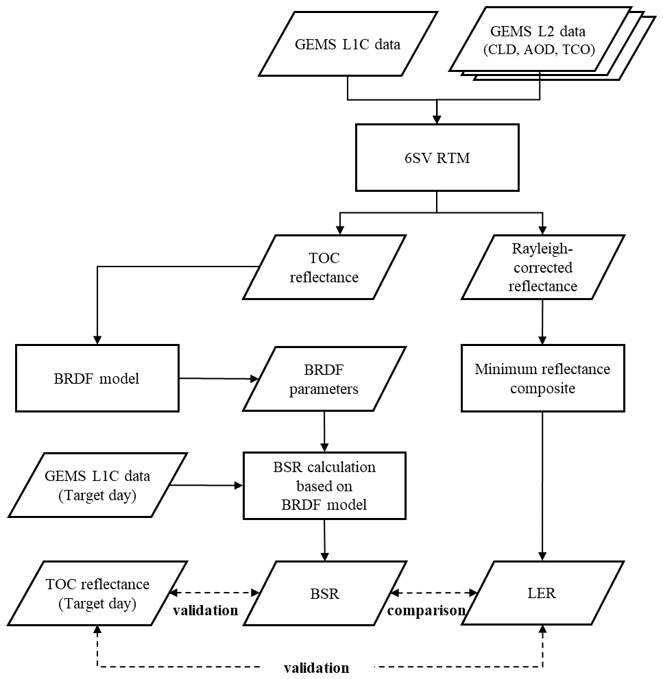
Figure 1 depicts a comprehensive flowchart of the BSR retrieval algorithm, which comprises two primary steps: (1) atmospheric correction and (2) BRDF modeling and BSR retrieval. The top-of-canopy (TOC) reflectance from GEMS represents the actual surface reflectance derived through atmospheric correction when AOD, CLD, and O3T products are available. To evaluate the applicability of the BSR derived in this study, validations were performed against the GEMS TOC data as reference data. Additionally, a comparison was made with the LER data generated using the minimum reflectance method which is used for a variety of LER datasets (Kleipool et al., 2008; Koelemeijer et al., 2003; Tilstra et al., 2017) and was first introduced in the work of Eck et al. (1987). GEMS BSR and LER were validated against the GEMS TOC data to compare their accuracy, followed by a direct comparison between BSR and LER. The detailed methodology and underlying assumptions are provided in the subsequent subsections.
3.1 Atmospheric correction
Atmospheric correction plays a pivotal role in satellite remote sensing by rectifying distortions caused by atmospheric effects, which can vary based on different geometries and atmospheric conditions. These atmospheric effects introduce significant uncertainties when the Earth’s surface is observed using satellite imagery. Thus, atmospheric correction is crucial for accurately determining surface reflectance. In most satellite data-processing methods, atmospheric correction is achieved using radiative transfer models (RTMs). Top-of-atmosphere (TOA) reflectance can be calculated using the atmospheric correction coefficients derived from the RTM; it is possible to calculate the TOC reflectance from the TOA reflectance. The Second Simulation of a Satellite Signal in the Solar Spectrum – Vector (6SV) RTM (Vermote et al., 2006) was employed for atmospheric correction, which was utilized in MODIS, the Visible Infrared Imaging Radiometer Suite (VIIRS) (Roger et al., 2016), and the Geostationary Operational Environmental Satellite (GOES) (Peng and Yu, 2020) data. The 6SV RTM divides the wavelength into intervals of 2.5 nm and computes the scattering and absorption effects in the atmosphere caused by aerosols and their geometric components. By employing the three atmospheric correction coefficients (xap, xb, and xc) derived from the 6SV RTM, the TOC reflectance can be calculated from the TOA reflectance. The surface reflectance was then calculated from the TOA reflectance, as expressed in Eq. (1). The atmospheric correction coefficients xap, xb, and xc can be computed using Eqs. (2), (3), and (4), where they represent the inverse of the transmittance, scattering term of the atmosphere, and spherical albedo, respectively. In these equations, , , θs, θv, ϕ, T↑(θs), T↓(θv), Tg, and S denote TOC reflectance, TOA reflectance, solar zenith angle (SZA), viewing zenith angle (VZA), relative azimuth angle (RAA), atmospheric transmittance (sun to target), atmospheric transmittance (target to sun), total gas transmittance, and spherical albedo, respectively.
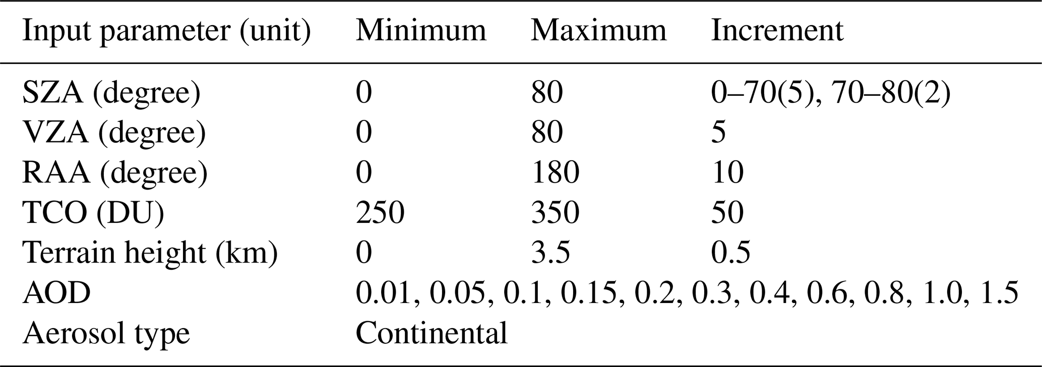
Although the RTM offers high accuracy in surface reflectance calculations, its computational complexity and time requirements are significant. To address this challenge, surface reflectance algorithms often use pre-simulated lookup tables (LUTs) generated using RTMs under various conditions. During LUT configuration, careful selection of input variables is crucial, as they directly impact the accuracy of atmospheric correction and surface reflectance calculations. In alignment with the characteristics of GEMS, six input variables were chosen for LUT construction: SZA, VZA, RAA, TCO, AOD, and terrain height. Table 1 outlines the range and intervals of these input variables for LUT construction with reference to previous studies on LUT-based surface reflectance calculations (Peng and Yu, 2020; Lee et al., 2020). Nevertheless, even with detailed interval adjustments, rapid changes at high angles can lead to discontinuities and degradation of the surface reflectance. Therefore, to ensure smooth and accurate results when calculating the surface reflectance based on the LUT, real-time interpolation was performed for all input components (SZA, VZA, RAA, TCO, AOD, and terrain height).
3.2 BSR retrieval through BRDF modeling
The computation of surface reflectance through atmospheric correction presents a significant limitation: its effectiveness is restricted to cloud-free regions and is influenced by the observational geometry at the time of measurement. Consequently, there is a critical need for a methodology capable of simulating the surface reflectance across diverse angular conditions to accurately compute the BSR. Thus, prior studies that required the simulation of surface reflectance at various angles, such as albedo calculations, have characterized the anisotropic properties of surfaces by utilizing the BRDF model (Gao et al., 2003; Wen et al., 2018). BRDF models can be classified into three categories: physical, empirical, and semi-empirical. Although a physical model can express the inherent physical meaning of each parameter mathematically, its versatility is limited because of its computationally intensive nature. The empirical model utilizes observation-based empirical formulas, making it suitable for situations with limited observations; however, it requires a substantial number of observations and does not elucidate the underlying physical background. Consequently, semi-empirical BRDF models are widely employed in satellite remote sensing.
In this algorithm, the semi-empirical Roujean bidirectional reflectance distribution function (BRDF) model (Roujean et al., 1992) was utilized for BRDF modeling. The Roujean BRDF model defines surface reflectance as a combination of isotropic, geometric, and volumetric scattering components. It comprises two physical kernels (f1 and f2) and three empirical coefficients (K0, K1, K2; BRDF parameters) that describe the mechanism of each component, as shown in Eq. (5). The two physical kernels of the Roujean BRDF model were defined under the assumption of irregularly spaced rectangular protrusions on a flat ground surface, neglecting all shadow interactions. The two physical kernels are calculated based on the angular component at the time of the observation (formulas are detailed in Roujean et al., 1992).
The observed surface reflectance can be decomposed into two kernels and three variables, as described by Eq. (5). Since the two kernels can be computed from the angular components, the BRDF parameters which characterize the anisotropic reflection based on multiple observations collected over a synthesis period can be calculated using the least squares method. This method assumes a relatively stable anisotropic reflection behavior of the surface over short periods in the absence of significant disturbances such as forest fires or floods. Therefore, these variables can be applied within a short time frame, enabling the simulation of surface reflectance under clear-sky conditions across all angular configurations within the target scene. Consequently, once the BRDF parameters are computed by providing solely the angular component of the observed target scene, the BSR at any angle can be simulated.
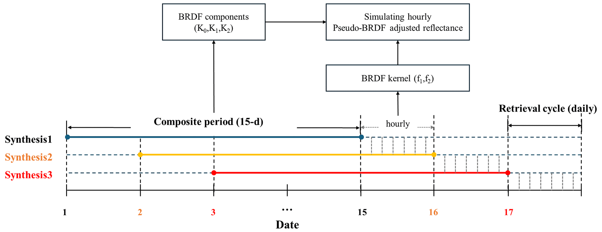
In this algorithm, the target scene refers to the day following the completion of BRDF synthesis. Figure 2 illustrates the synthesis period of 15 d and the retrieval cycle used for BRDF modeling in the algorithm. The BRDF synthesis period spans 15 d and encompasses all observed hourly data within this time frame. This enabled the application of the resulting BRDF composites to the subsequent day, allowing for the simulation of hourly BSR based solely on the angular components observed the following day. These BRDFs were generated in a daily cycle, with the synthesis period shifted by 1 d. This methodology enables comprehensive reconstruction of the surface reflection characteristics at various angles, offering valuable insights into the directional reflectance behavior of the surface.
Insufficient observations lead to uncalculated BRDF parameters, resulting in missing BSR values, which are crucial for other L2 algorithms. To address this, a gap-filling process utilizing the “age” variable in BRDF modeling was implemented. This method uses previously calculated BRDF parameters up to 5 d of age to fill gaps when current parameters are unavailable. In this process, the age variable was defined and utilized, indicating how many days old the BRDF parameters used for gap filling are. For example, if BRDF parameters from 3 d ago are used, the age variable is assigned a value of 3. If the BRDF parameters are not be calculated the next day and the same date's BRDF parameters are used, the age variable is assigned a value of 4. Conversely, if new BRDF parameters are calculated, the age variable is reset to 0. If the age variable exceeds 5, the parameters are no longer used. To summarize, the age variable indicates the number of days since the last valid BRDF calculation, reset to 0 after 5 d or once the BRDF parameter is calculated.
3.3 GEMS LER assumption
The GEMS LER was derived from the Rayleigh-corrected reflectance, which was computed by assuming a Rayleigh atmosphere to eliminate aerosol effects during atmospheric correction. This calculation utilized the same LUT as the TOC reflectance calculation with the AOD set to zero. It was assumed that the formulas for calculating the LER and 6SV-based atmospheric corrections were nearly identical. Equations (6) and (7) summarize these formulas, where ρ6SV and ρLER represent the 6SV-based TOC and LER calculation formulas (Kleipool et al., 2008), respectively. In this study, ρ6SV was designated as the Rayleigh-corrected reflectance for the scene. The GEMS LER was determined to be the minimum reflectance over a 15 d period to match the BRDF synthesis period. A 15 d synthesis period was also found by Park et al. (2023) to be an effective balance between minimizing cloud contamination and maintaining consistent surface reflectance in the application of the minimum reflectance method. The resulting GEMS LER was used for additional gap filling in cases where the GEMS BSR was consistently missing despite utilizing the age variable.
4.1 BSR validation with TOC reflectance
4.1.1 Quantitative validation of GEMS BSR and LER
The purpose of the BSR data was to simulate reflectance as similarly as possible to the TOC reflectance calculated based on actual observation conditions in advance and use the TOC reflectance as an input for other L2 products. Therefore, verification was performed by comparing the TOC calculated after the L2 products (CLD, AOD, and TCO) utilized for the TOC reflectance calculation were produced with the BSR simulated in advance as a reference value. We have produced TOC reflectance and BSR data for 1 year, from 1 January to 31 December 2021, and performed BSR verification based on these data.
The BSR validation was limited to instances of high quality, with the quality criteria defined based on the number of observations and RMSE during the BRDF modeling. The number of observations refers to the number of valid pixels used within the same pixel for BRDF modeling, whereas the BRDF RMSE signifies the RMSE between the actual observed reflectance and simulated reflectance. In this context, the simulated reflectance represents the value that emulates the reflectance back to the angular component of the actual observation condition based on the BRDF parameters derived through BRDF modeling. The GK-2A AMI albedo product establishes the standard for good-quality BSR, requiring seven or more observations and a BRDF RMSE of 0.07 or lower (Lee et al., 2020). In addition, MODIS albedo considers an RMSE value within 10 % of the channel-specific reflectance distribution as indicative of good quality (Roman et al., 2013). Consequently, the BSR quality criterion in this study was defined as requiring seven or more observations and a BRDF RMSE of 0.03 or lower, given that the GEMS 440 nm BSR typically reaches a maximum value of 0.3. All subsequent quantitative analyses were conducted exclusively using good-quality data.
Figure 3 presents a comparison between GEMS BSR and GEMS LER using the GEMS TOC reflectance as a reference, encompassing all hourly data from January to December 2021. The comparison revealed that the GEMS BSR simulated the TOC values more closely than the GEMS LER. To quantify this comparison, we evaluated the RMSE, relative RMSE (rRMSE), and bias. The rRMSE was computed by dividing the RMSE by the average reference data value, which served as an indicator of overall relative accuracy. For the GEMS BSR, the RMSE was 0.015, the rRMSE was 19.38 %, and the bias was 0.002. Conversely, for GEMS LER, the RMSE was 0.017, the rRMSE was 22.17 %, and the bias was −0.009. These results suggest that the GEMS BSR exhibited a lower rRMSE of 3 % and a lower bias value of 0.007 (based on the absolute value), indicating superior simulation performance compared to the minimum reflectance.
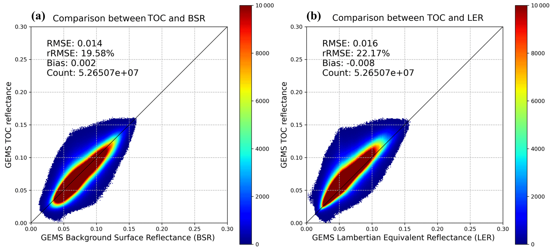
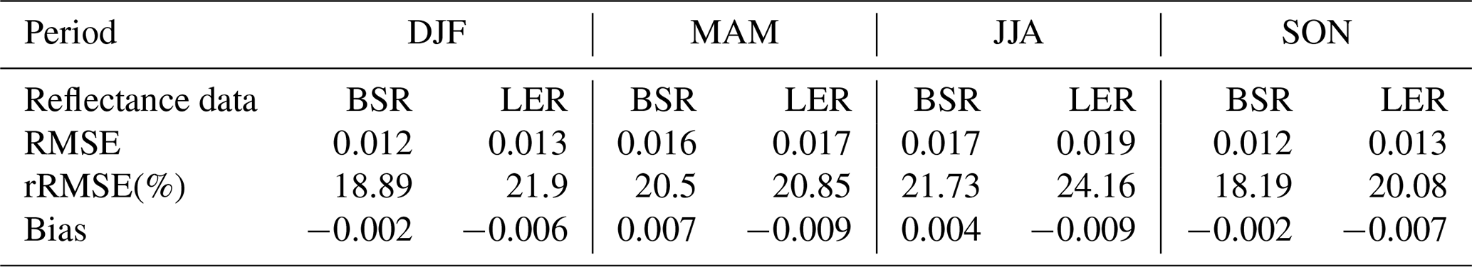
Table 2 presents a quantitative comparison between GEMS BSR and LER for each season. The seasons are represented as DJF, MAM, JJA, and SON, corresponding to December–January–February, March–April–May, June–July–August, and September–October–November, respectively, and denote winter, spring, summer, and fall, respectively. The RMSE, rRMSE, and bias values for BSR are 0.012, 0.016, 0.017, and 0.012 for RMSE; 18.89 %, 20.5 %, 21.73 %, and 18.19 % for rRMSE; and −0.002, 0.007, 0.004, and −0.002 for bias, respectively, in the order of winter, spring, summer, and fall. For the GEMS LER, the RMSE values were 0.013, 0.017, 0.019, and 0.013, respectively; the rRMSE values were 21.9 %, 20.85 %, 24.16 %, and 20.08 %, respectively; and the bias values were −0.006, −0.009, −0.009, and −0.007 for each season, respectively. BSR exhibited lower RMSE, rRMSE, and bias values than LER, indicating the superior simulation performance of BSR in all seasons. Both data sources show the highest RMSE in summer compared to the other seasons. However, the difference in rRMSE compared to RMSE did not change much across the seasons because the reflectance in winter and fall was relatively lower than that in spring and summer.
Table 2Seasonal quantitative comparison of GEMS BSR and LER with GEMS TOC reflectance as reference (DJF means December–January–February, MAM means March–April–May, JJA means June–July–August, and SON means September–October–November).
4.1.2 Qualitative validation of GEMS BSR and LER
After completing the quantitative analysis, we conducted a qualitative comparison between the GEMS TOC, BSR, and LER to evaluate their spatial distribution. Figure 4 illustrates this qualitative analysis, with each row displaying the GEMS TOC, BSR, LER, and the difference between BSR and LER relative to TOC for the same date and time. Figure 4a–d represent the calculations for 20 February at 02:45 UTC, 1 May at 03:45 UTC, 9 August at 02:45 UTC, and 10 November 2021 at 05:45 UTC.
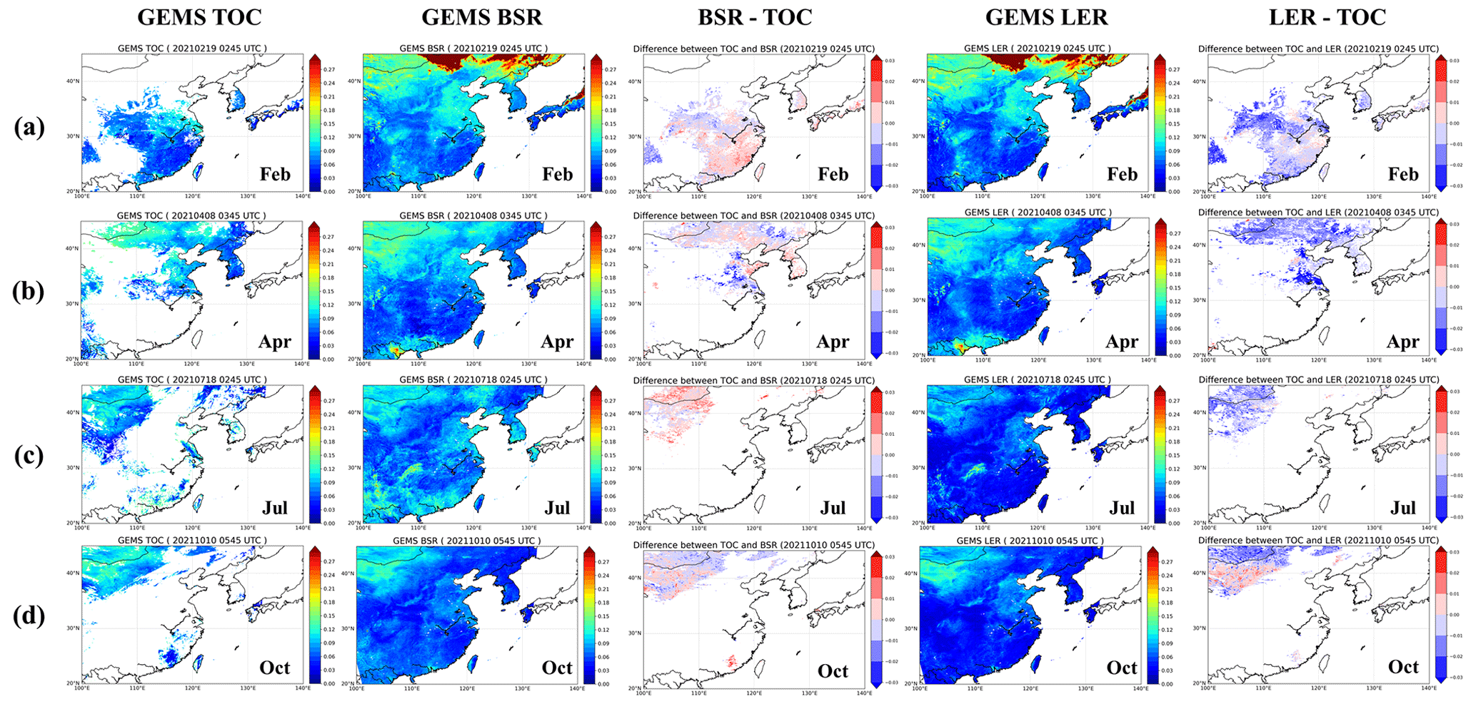
Figure 4Qualitative comparison of GEMS TOC, BSR, and LER. (a) GEMS TOC; (b) GEMS BSR; (c) difference between BSR and TOC; (d) GEMS LER; (e) difference between LER and TOC.
TOC reflectance is applicable only under clear-sky conditions and can be computed only in areas where all necessary inputs, such as AOD and TCO, are available, resulting in numerous areas with missing data. The difference between the BSR and LER data in terms of TOC was examined only for areas where the GEMS TOC was calculated. For BSR, a mixed trend of underestimation and overestimation was observed; however, in July, most areas exhibited higher reflectance than TOC. In contrast, the LER showed a consistent trend of underestimation in most areas, except for October, which aligns with our expectations. However, in October, LER exhibited a similar trend to BSR, but with a stronger magnitude, indicating that even applying minimum reflectance can result in higher values than those from BRDF modeling. This again highlights the importance of considering the BRDF when calculating land surface reflectance.
A qualitative analysis was also conducted between the BSR and LER for areas where TOC reflectance was not calculated. The greatest difference between the two sources was observed in July (summer), compared with the spring, summer, and fall results in February, April, and October, respectively. In July, the LER consistently simulated lower reflectance than the BSR across the entire region, particularly in the central and eastern parts of the country. These areas experience frequent cloud cover and fog throughout the year, making it challenging to obtain clear-sky pixel counts during all seasons. However, this challenge is exacerbated in summer months when clouds are more prevalent. If clouds are not detected in the cloud product, high reflectance can be inputted into the BRDF model and mistakenly interpreted as clear-sky reflectance, leading to simulation errors. Conversely, the minimum reflectance technique tends to adopt the lowest reflectance value during the synthesis period, even in the presence of clouds and shadows, resulting in a lower reflectance.
4.2 Analyzing surface reflectance variation across land types
4.2.1 Time series consistency analysis by land types
To assess the simulation performance based on the time series of the BSR, we analyzed the time series stability across four land types (grassland, cropland, shrubland, and urban) using MODIS land cover data. The dataset utilized in this study is derived from the MODIS/Terra+Aqua Land Cover Type Yearly L3 Global 0.05Deg CMG V061 (MCD12C1) product (Strahler et al., 1999). The classification follows the International Geosphere-Biosphere Programme (IGBP) scheme within the MODIS land cover dataset. Specifically, we employed the land cover data from the year 2021. Figure 5 illustrates the time series of GEMS TOC, BSR, and LER analyzed for each land type, where panels (a)–(d) correspond to grassland, cropland, shrubland, and urban areas, respectively. These values were averaged over all good-quality pixels for each land type based on MODIS land cover. In this analysis, the LER was excluded if it did not meet the criteria for good-quality BSR to mitigate the impact of clouds.
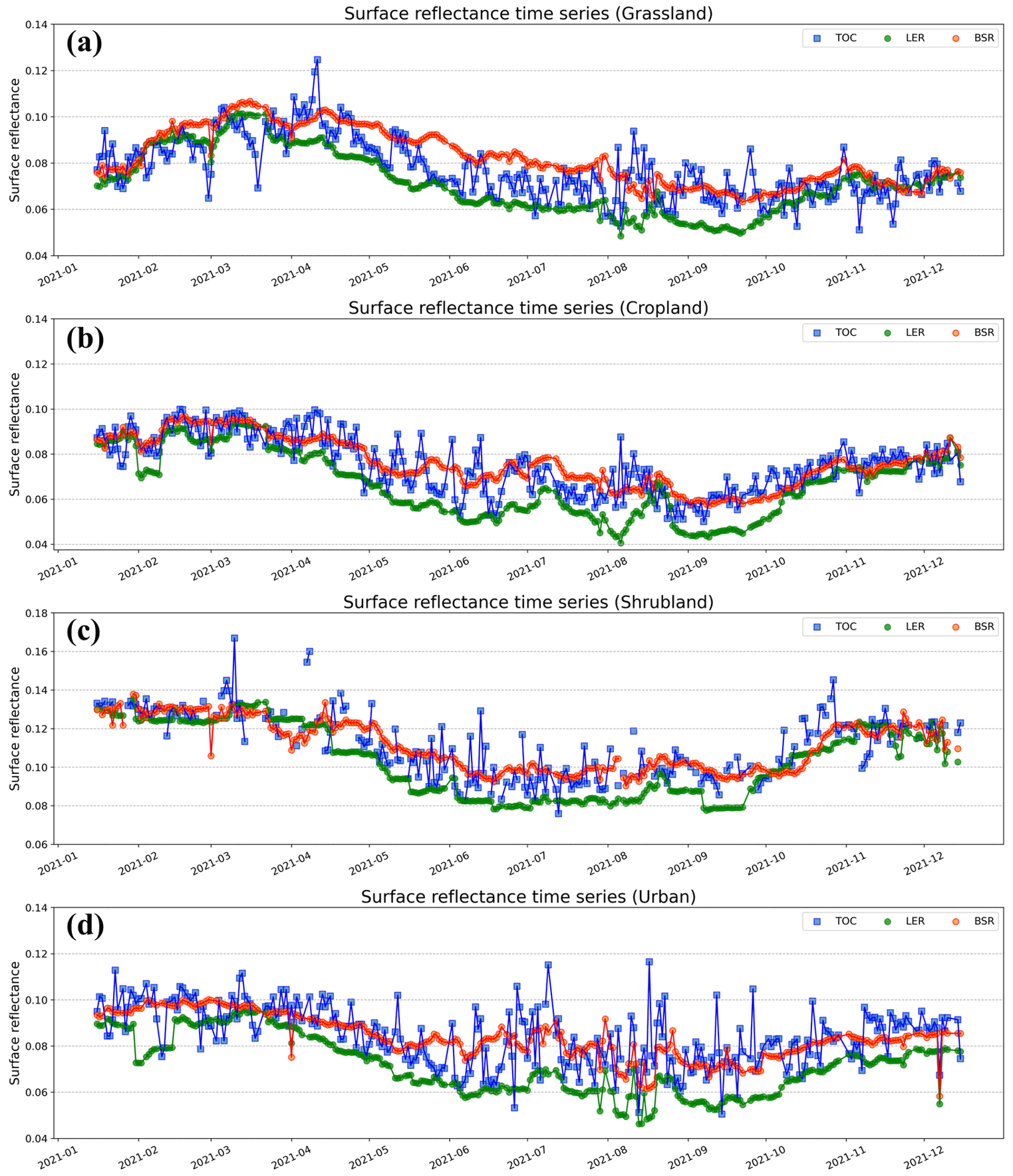
Figure 5Time series distribution of TOC, BSR, and LER by land type. (a) Grassland; (b) cropland; (c) shrubland; (d) urban.
The blue squares in Fig. 5 represent the reference TOC values, the green circles represent the LER values, and the red circles represent the BSR values. The analysis indicated that for all four land types, both BSR and LER exhibited stable time series distributions, mirroring the TOC trend. However, when compared with the TOC distribution, the BSR appeared to track the trend slightly better than the LER across all land types. This was most evident between May and October, as LER consistently simulated a lower reflectance than TOC. In addition, in the shrublands during this period, LER tended to consistently adopt nearly identical values, whereas TOC and BSR showed variability in reflectance.
However, for grassland, the trend was opposite to that of LER, with BSR consistently simulating a higher reflectance than TOC during the summer months. While there was a clear tendency for the BSR to simulate higher reflectance, this was similar to the observed range of the TOC reflectance distribution and was not considered a significant error. Therefore, this analysis confirms that the BSR tends to follow the TOC reflectance more reliably than the LER over time.
4.2.2 Surface reflectance influence on AOD variability in cropland and urban areas
Li et al. (2012) provided quantitative figures for the variability in the AOD output with reflectance changes in the blue channel. The analysis focused on different AOD ranges (AOD < 0.4, 0.4 < AOD < 0.8, 0.8 < AOD < 1.2, 1.2 < AOD < 1.6, 1.6 < AOD < 2.0) according to the degree of ground reflectance change (ranging from 0.001 to 0.05). To quantitatively evaluate the advantage of BSR over LER in terms of AOD, we reanalyzed the results of Li et al. (2012) using the findings of this study. The analysis was limited to the AOD value of 0.4, and the variability was analyzed and converted into percent error using a quadratic regression equation based on the change in AOD value corresponding to the change in ground surface reflectance as presented in the study. In this context, the amount of AOD change refers to the difference in AOD values when using BSR and LER data compared to when using TOC, assuming that the AOD output value when using TOC is 0.4. The percent error of AOD can be calculated using Eq. (8), where AODreference is the AOD value when using TOC (AOD is fixed at 0.4 in this study) and AODobserved is the AOD value when using BSR and LER. However, as Li et al.'s 2012 study only analyzed urban and rural areas in China, it also focused on cropland and urban land types.
Figure 6 presents the seasonal RMSE, bias, and AOD percent error results, with Fig. 6a and b representing the results for cropland and urban areas, respectively. In each panel, the first to third columns denote the RMSE, bias, and AOD percentage error based on TOC, respectively. Both RMSE and bias values were expressed by multiplying the calculated value by 100. Throughout all seasons, BSR consistently exhibited lower RMSE and bias values than LER. LER tended to show a negative bias, whereas BSR showed a positive bias. Interestingly, both datasets demonstrated high RMSE values in summer, with the BSR tending to overestimate and the LER tending to underestimate. This inverse behavior is in line with the trends observed in the previous time series graphs. Specifically, in the cropland and urban areas, the BSR maintained a low bias of 0.0022 or less, except in summer. In contrast, LER exhibited a negative bias of more than 0.084 in most cases, except in winter in the croplands.
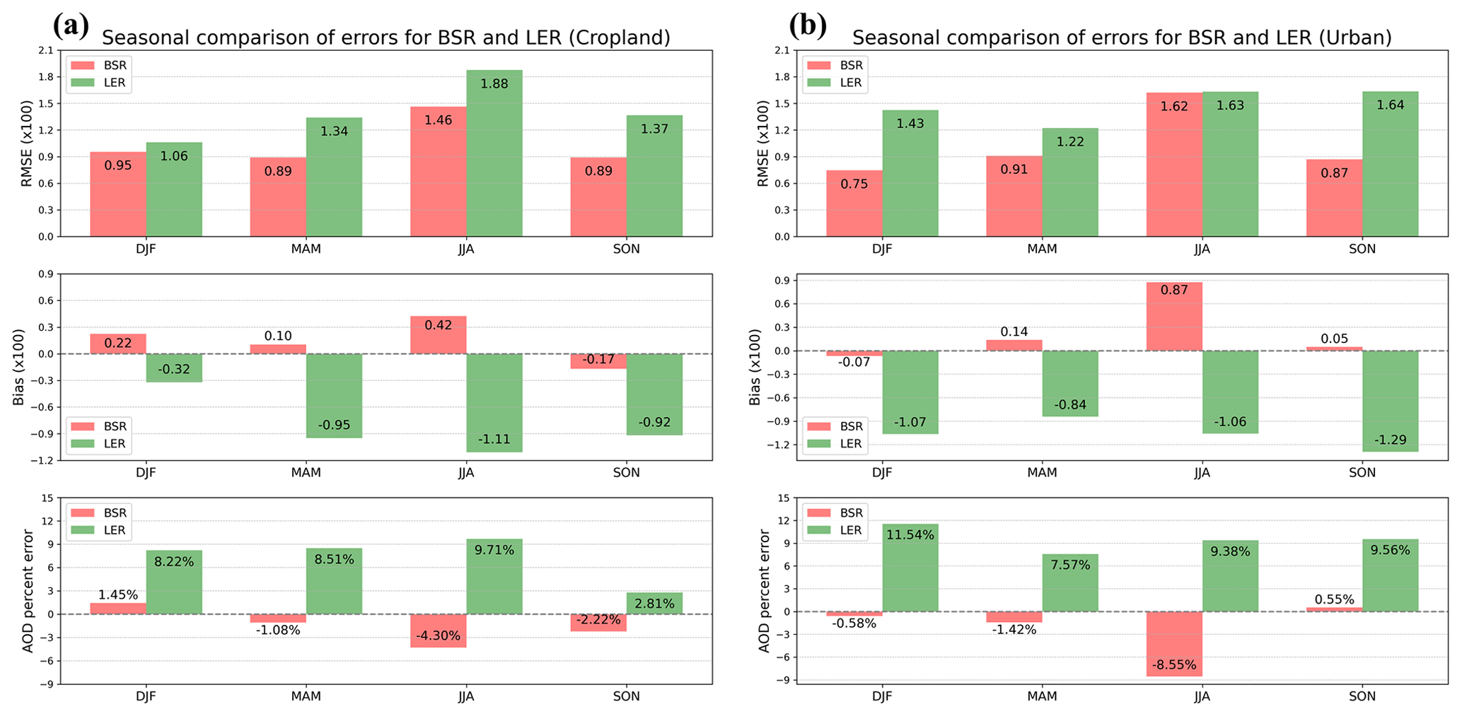
Figure 6RMSE and bias in cropland and urban land types by season, as well as the resulting AOD percent error. (a) Cropland; (b) urban.
Analysis of the AOD percent error revealed that LER exhibited higher error values than BSR across all seasons. Due to the high RMSE values observed in summer for both datasets, the AOD percentage error also tended to increase during this season. However, excluding summer, BSR consistently demonstrated better AOD percentage error values than LER, with improvements of up to 7.4 % in spring for croplands and 10.9 % in winter for urban areas. These findings suggest that the BSR has the potential to generate more stable AOD outputs than the LER.
4.3 Accuracy evaluation using ground measurements
To conduct a thorough and precise validation of GEMS BSR, comparisons and validations were performed using RadCalNet ground observations. RadCalNet data utilized ground reflectance observations from the BSCN sites, and only data within 15 min of the observation time were used because of the sensitivity of ground reflectance to temporal changes. In addition, various LER databases currently available in the field were used for verification to assess the performance of the BSR. These include the OMI LER, GLER, TROPOMI DLER, GOME-2 LER, and SCIAMACHY LER. OMI GLER and DLER considered surface BRDF effects and conducted observations over the study area, mostly between 03:00 and 05:00 UTC. Therefore, the validation was limited to data from 03:45–05:45 UTC based on RadCalNet. For TROPOMI DLER, the BRDF effect on the viewing geometry can be accounted for using four coefficients. These coefficients can be derived from the LER and converted into the DLER using the following Eq. (9): for comparison and validation, the GEMS VZA at 04:45 UTC was multiplied by the corresponding coefficients to calculate the TROPOMI DLER. θv in the formula is the GEMS VZA, and c0 to c4 are the TROPOMI DLER coefficients.
Figure 7 illustrates the results of the validation of the LER databases, including the GEMS BSR, based on RadCalNet observations. Figure 7a compares OMI GLER, TROPOMI DLER, and GEMS BSR with the RadCalNet data, whereas Fig. 7b compares OMI, GOME-2, SCIAMACHY LER, and GEMS BSR. The RMSE, rRMSE, and bias between each dataset and RadCalNet are presented in Table 3. The analysis revealed that the RMSE values of OMI GLER, TROPOMI DLER, and GEMS BSR were 0.018, 0.009, and 0.007, respectively, with rRMSE values of 21.42 %, 10.57 %, and 8.59 %, respectively, and bias values of −0.008, −0.006, and 0.001, respectively. These results indicate that the GEMS BSR is more accurate than the OMI GLER and TROPOMI DLER in terms of RMSE, rRMSE, and bias, with a 13 % improvement over the OMI GLER and 2 % improvement over the TROPOMI DLER based on the rRMSE.
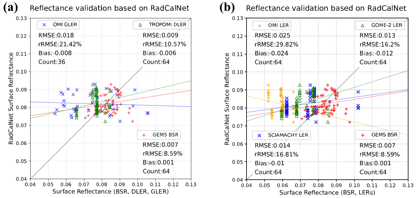
Figure 7Validation of surface reflectance databases using RadCalNet observations. (a) Validation of OMI GLER, TROPOMI DLER, and GEMS BSR. (b) Validation of OMI LER, GOME-2 LER, SCIAMACHY LER, and GEMS BSR.
Furthermore, OMI GLER exhibited a significantly wider distribution than the RadCalNet reflectance occurrence range, whereas TROPOMI DLER had almost the same reflectance adopted multiple times. This suggests that similar DLER values were calculated multiple times in the same month because of the nature of the LER database data, as the GEMS satellite is geostationary and the VZA varies little at the same observation time. Similar trends were observed when comparing the three LER databases (OMI, GOME-2, and SCIAMACHY), with RMSE values of 0.025, 0.013, and 0.014; rRMSE values of 29.82 %, 16.2 %, and 16.81 %; and bias values of −0.024, −0.012, and −0.01, respectively.
In conclusion, considering BRDF effects, such as BSR, GLER, and DLER, rather than utilizing LER databases for alternative land surface reflectance calculations can provide more realistic reflectance simulations, with GEMS BSR demonstrating the best performance among the six sources analyzed.
Table 3GEMS BSR and LER database accuracy evaluation based on RadCalNet ground observation data.
4.4 Intercomparison between GEMS BSR and LER database (OMI GLER, TROPOMI DLER)
TROPOMI and OMI performed observations between 03:45 and 05:45 UTC during GEMS observations in the study area, with the largest number of observations occurring at 04:45 UTC. Therefore, a comparison of the GEMS BSR with the DLER and GLER was conducted at 04:45 UTC. Consistent with the analysis in the previous section, OMI GLER was calculated using only the data within 15 min of the GEMS observations, whereas TROPOMI DLER was calculated using GEMS VZA. Figure 8 compares GEMS TOC with GEMS BSR, TROPOMI DLER, and OMI GLER. Figure 9 presents the intercomparison between BSR and OMI GLER, as well as BSR and TROPOMI DLER.
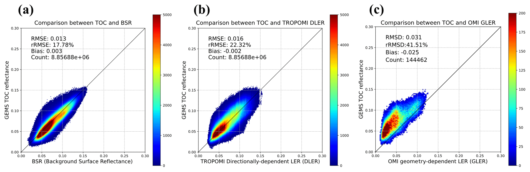
Figure 8Distribution density plot of GEMS BSR, TROPOMI DLER, and OMI GLER based on GEMS TOC observations. (a) GEMS BSR; (b) TROPOMI DLER; (c) OMI GLER.
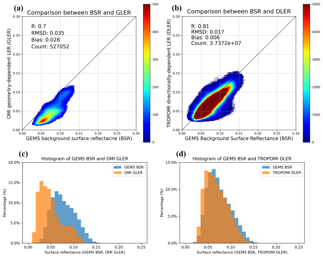
Figure 9Quantitative comparison of GEMS BSR, TROPOMI DLER, and OMI GLER value distributions. (a) Density plot of BSR and GLER; (b) density plot of BSR and DLER; (c) histogram of BSR and GLER; (d) histogram of BSR and DLER.
Compared to GEMS TOC, BSR, DLER, and GLER, the rRMSE values were 17.78 %, 22.32 %, and 41.51 %, with biases of 0.003, −0.002, and −0.025, respectively. The GEMS BSR tended to exhibit a positive bias, whereas the DLER and GLER tended to display a negative bias. When analyzing the graph distribution, we observed a significant clustering of values below 0.05 in the OMI GLER data. Owing to the inherent differences in assumptions between the GLER and DLER databases and BSR, direct quality verification through comparison is challenging. However, this suggests that the BSR is capable of simulating reflectance that closely aligns with TOC reflectance, indicating its potential for realistic reflectance simulation.
Figure 9 shows a density plot and histogram comparing BSR with OMI GLER and TROPOMI DLER. Panels (a) and (c) show a comparison with GLER, whereas panels (b) and (d) show a comparison with DLER. The correlation coefficient (R) for GLER was 0.7, with a root mean square difference (RMSD) of 0.035 and a bias of 0.028. For DLER, the R, RMSD, and bias were 0.81, 0.017, and 0.006, respectively, indicating a strong positive correlation for both data sources. The histograms reveal that the distributions of the DLER and BSR values are quite similar, whereas GLER is more concentrated at low ground reflectance compared to BSR. This suggests that BSR yields results that are more akin to those of DLER than those of GLER. Although the BSR showed relatively high values when the GLER and DLER were near 0.05 in the density plot distribution, it was not considered a significant error owing to its small magnitude.
Figure 10 presents a qualitative comparison of the reflectances of GEMS BSR, TROPOMI DLER, and OMI GLER. The columns represent BSR, DLER, and GLER from left to right, and rows (a)–(c) represent dates 26 March, 23 June, and 23 September 2021, respectively. From the qualitative comparison, we can see that BSR and DLER have fairly similar distributions of values, whereas GLER tends to produce relatively low reflectance values in China compared with the other two datasets. However, as mentioned in the previous analysis, the BSR simulates a slightly higher reflectance during the summer months, with its values being relatively higher than those of the other dates. However, all three datasets had very similar distributions, albeit with slight differences in their absolute values. This analysis provides further evidence that the BSR effectively simulates the reflectance properties of the ground surface, similar to the DLER and GLER.
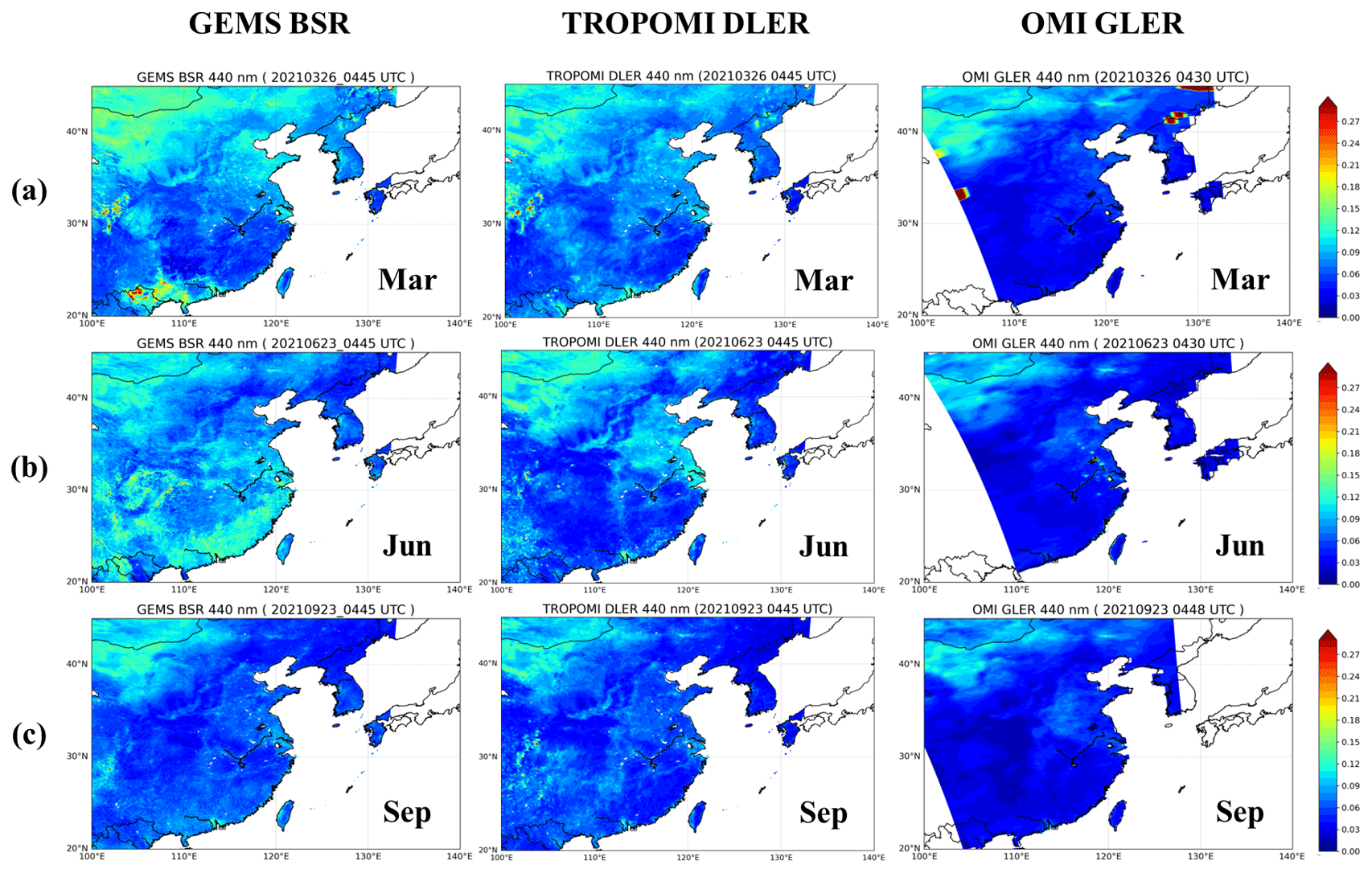
Figure 10Qualitative comparison of GEMS BSR, TROPOMI DLER, and OMI GLER distributions in March, June, and September. The table rows correspond to GEMS BSR, TROPOMI DLER, and OMI GLER, in that order. (a) 26 March 2021; (b) 23 June 2021; (c) 23 September 2021.
This study represents the first practical application of BSR as an alternative output to resolve the output precedence dilemma between land surface reflectance and other L2 outputs applied to GEMS at 440 nm, evaluating its feasibility for operational use. This concept, often referred to as BSR, involves a preliminary simulation of realistic ground reflectance before atmospheric correction. This simulation was based on variables reflecting the BRDF effect on the ground surface calculated through BRDF modeling. BSR overcomes the limitation of underestimating ground reflectance that may occur with the minimum reflectance technique.
Various analytical methods were employed to evaluate the simulation performance of the BSR. The purpose of the BSR output was to simulate the TOC reflectance more realistically in advance using the actual observed values required for atmospheric corrections, such as CLD, AOD, and TCO. Therefore, TOC reflectance was used as a reference for evaluating the simulation performance of the BSR. The simulation performance of the GEMS BSR was 3 % more accurate than that of the GEMS LER data in terms of the rRMSE over the entire study period based on TOC. The bias was −0.007 for LER and 0.002 for BSR, indicating an improvement in the underestimation of surface reflectance when BSR is applied.
The stability of the BSR calculation over time was also verified by analyzing the trend of the reflectance distribution according to MODIS land cover. For the selected terrains (grassland, cropland, shrubland, and urban), the BSR tracked the TOC trend better than the LER. In summer, a tendency for BSR to be overestimated compared to TOC was observed in grasslands. In contrast, LER was significantly underestimated compared to BSR in all land types, especially between May and September, confirming the temporal stability of the BSR.
Furthermore, after validation with TOC, comparison and validation were performed with other LER databases available in the field based on ground observations from RadCalNet. The OMI, GOME-2, SCIAMACHY LER, OMI GLER, and TROPOMI DLER data were used in the analysis. For the RadCalNet-based land surface reflectance validation, GEMS BSR exhibited the best simulation performance among the six databases, with an rRMSE of 8.59 % and a bias of 0.001. When comparing the results of OMI GLER and LER validation, OMI GLER had an rRMSE of 21.42 % and a bias of −0.008, while OMI LER had an rRMSE of 29.82 % and a bias of −0.024. This indicates that accounting for surface BRDF effects in the calculation of ground reflectance provides a more realistic reflectance simulation.
A comparison of GEMS BSR with TROPOMI DLER and OMI GLER based on TOC reflectance revealed that BSR tended to exhibit a positive bias, whereas DLER and GLER tended to display a negative bias. Despite the challenges in directly verifying the quality, the analysis suggests that BSR can simulate reflectance closely aligned with TOC reflectance, indicating its potential for realistic reflectance simulation. Additionally, the comparison between DLER and GLER based on BSR showed strong positive correlations, with BSR exhibiting distributions more similar to those of DLER. Overall, the BSR demonstrated the capability to effectively simulate ground surface reflectance properties, similar to the DLER and GLER.
Although, limitations exist, such as the challenge of capturing sudden changes in surface characteristics such as snow or ice cover. In addition, to enhance stability, we designed a method to use CAMS AOD data in the absence of GEMS AOD, acknowledging the presence of some bias. Despite this limitation, we prioritized maintaining a stable dataset. Our research is pioneering in its application to BRDF modeling and evaluation in hyperspectral observation satellite studies. We are committed to further refining our approach and will strive to address these biases in future research to improve calculation accuracy.
In conclusion, our study demonstrated that BSR can effectively simulate realistic reflectance, surpassing the minimum reflectance approach used in many existing studies. By combining the high temporal and spatial resolution of GLER with the BRDF considerations of DLER, we laid the foundation for improved accuracy in the AQ output. Our findings suggest that the utilization of BSR, a dataset reflecting realistic reflectance with BRDF effects, can enhance various climate analysis studies, marking a significant advancement in the field.
The data used in this study are accessible from the following links: GEMS level 2 data (AERAOD, TCO, CLD) (https://nesc.nier.go.kr/en/html/datasvc/index.do, NIER, 2024); OMI/Aura global geometry-dependent surface LER (GLER) (https://disc.gsfc.nasa.gov/datasets/OMGLER_003/summary?keywords=OMIGLER, last access: 17 September 2024, NASA,Goddard Earth Sciences Data and Information Services Center (GES DISC), https://doi.org/10.5067/AURA/OMI/DATA2032, Joiner et al., 2019); TROPOMI directionally dependent Lambertian-equivalent reflectivity (DLER) (https://www.temis.nl/surface/albedo/tropomi_ler.php, KNMI, 2024); OMI surface LER database (https://www.temis.nl/surface/albedo/omi_ler.php, last access: 17 September 2024, KNMI; Kleipool et al., 2008); SCIAMACHY surface LER database (https://www.temis.nl/surface/albedo/scia_ler.php, last access: 17 September 2024, KNMI; Tilstra et al., 2017); GOME-2 surface LER database (https://www.temis.nl/surface/albedo/gome2_ler.php, last access: 17 September 2024, KNMI, AC SAF; Tilstra et al., 2017); CAMS global atmospheric composition forecasts dataset (https://ads.atmosphere.copernicus.eu/, ECMWF, 2024); and RadCalNet data (https://www.radcalnet.org/, last access: 17 September 2024; Bouvet et al., 2019).
SS and KSH conceptualized and designed the study, collected and analyzed the data, and wrote the manuscript. SC and DJ contributed to the study design, conducted the statistical analysis, and critically reviewed the manuscript. JW and HK assisted in data interpretation and manuscript preparation. NK and SP provided expertise in experimental procedures and contributed to the data collection. UJ and HH contributed to the study design and provided intellectual input throughout the research process. All authors read and approved the final manuscript.
The contact author has declared that none of the authors has any competing interests.
Publisher’s note: Copernicus Publications remains neutral with regard to jurisdictional claims made in the text, published maps, institutional affiliations, or any other geographical representation in this paper. While Copernicus Publications makes every effort to include appropriate place names, the final responsibility lies with the authors.
This article is part of the special issue “GEMS: first year in operation (AMT/ACP inter-journal SI)”. It is not associated with a conference.
The authors acknowledge the contribution of the Environmental Satellite Center (ESC), National Institute of Environmental Research (NIER), for providing GEMS data. The GEMS data used in this study were provided by the GEMS algorithm team for validation and improvement research purposes.
This research was supported by a grant from the National Institute of Environmental Research (NIER), funded by the Korea Ministry of Environment (MOE) of the Republic of Korea (grant no. NIER-2024-04-02-028).
This paper was edited by Rokjin Park and reviewed by Meng Gao, Sang Seo Park, and one anonymous referee.
Baek, K., Kim, J. H., Bak, J., Haffner, D. P., Kang, M., and Hong, H.: Evaluation of total ozone measurements from Geostationary Environmental Monitoring Spectrometer (GEMS), Atmos. Meas. Tech., 16, 5461–5478, https://doi.org/10.5194/amt-16-5461-2023, 2023. a, b
Bouvet, M., Thome, K., Berthelot, B., Bialek, A., Czapla-Myers, J., Fox, N., Goryl, P., Henry, P., Ma, L., Marcq, S., Meygret, A., Wenny, B., and Woolliams, E.: RadCalNet: A radiometric calibration network for Earth observing imagers operating in the visible to shortwave infrared spectral range, Remote Sens., 11, 2401, https://doi.org/10.3390/rs11202401, 2019. a, b
Chen, L., Wang, R., Han, J., and Zha, Y.: Influence of observation angle change on satellite retrieval of aerosol optical depth, Tellus B, 73, 1–14, https://doi.org/10.1080/16000889.2021.1940758, 2021. a
Cho, Y., Kim, J., Go, S., Kim, M., Lee, S., Kim, M., Chong, H., Lee, W.-J., Lee, D.-W., Torres, O., and Park, S. S.: First atmospheric aerosol-monitoring results from the Geostationary Environment Monitoring Spectrometer (GEMS) over Asia, Atmos. Meas. Tech., 17, 4369–4390, https://doi.org/10.5194/amt-17-4369-2024, 2024. a, b
Choi, W., Moon, K.-J., Yoon, J., Cho, A., Kim, S.-k., Lee, S., Ko, D., Kim, J., Ahn, M., Kim, D.-R., Kim, S.-M., Kim, J.-Y. Nicks, D., and Kim, J.-S.: Introducing the geostationary environment monitoring spectrometer, J. Appl. Remote Sens., 12, 044005, https://doi.org/10.1117/1.JRS.12.044005, 2018. a
Choi, Y.-S., Kim, G., Kim, B.-R., Kwon, M.-J., Kim, Y., Yoon, J., Lee, D.-W., and Kim, J.: Geostationary Environment Monitoring Spectrometer (GEMS), Algorithm Theoretical Basis Document: Cloud Retrieval Algorithm, Tech. rep., Environmental Satellite Center, National Institute of Environmental Research, Ministry of Environment, https://nesc.nier.go.kr/en/html/satellite/doc/doc.do (last access: 17 September 2024), 2020. a
De Smedt, I., Theys, N., Yu, H., Danckaert, T., Lerot, C., Compernolle, S., Van Roozendael, M., Richter, A., Hilboll, A., Peters, E., Pedergnana, M., Loyola, D., Beirle, S., Wagner, T., Eskes, H., van Geffen, J., Boersma, K. F., and Veefkind, P.: Algorithm theoretical baseline for formaldehyde retrievals from S5P TROPOMI and from the QA4ECV project, Atmos. Meas. Tech., 11, 2395–2426, https://doi.org/10.5194/amt-11-2395-2018, 2018. a
Dickinson, R.: Land surface processes and climate–surface albedos and energy balance, Adv. Geophys., 25, 305–353, https://doi.org/10.1016/S0065-2687(08)60176-4, 1983. a
Eck, T., Bhartia, P., Hwang, P., and Stowe, L.: Reflectivity of Earth's surface and clouds in ultraviolet from satellite observations, J. Geophys. Res.-Atmos., 92, 4287–4296, https://doi.org/10.1029/JD092iD04p04287, 1987. a
ECMWF: Copernicus, https://ads.atmosphere.copernicus.eu/, last access: 17 September 2024. a
Frey, R., Ackerman, S., Liu, Y., Strabala, K. I., Zhang, H., Key, J., and Wang, X.: Cloud detection with MODIS. Part I: Improvements in the MODIS cloud mask for collection 5, J. Atmos. Ocean. Tech., 25, 1057–1072, https://doi.org/10.1175/2008JTECHA1052.1, 2008. a
Gao, C., Liu, Y., Wu, Z., Ma, L., Qiu, S., Li, C., Zhao, Y., Han, Q., Zhao, E., Qian, Y., and Wang, N.: An approach for evaluating multisite radiometry calibration of Sentinel-2B/MSI using RadCalNet sites, IEEE J. Sel. Top. Appl., 14, 8473–8483, https://doi.org/10.1109/JSTARS.2021.3102271, 2021. a
Gao, F., Schaaf, C., Strahler, A., Jin, Y., and Li, X.: Detecting vegetation structure using a kernel-based BRDF model, Remote Sens. Environ., 86, 198–205, https://doi.org/10.1016/S0034-4257(03)00100-7, 2003. a
Herman, J. and Celarier, E.: Earth surface reflectivity climatology at 340–380 nm from TOMS data, J. Geophys. Res.-Atmos., 102, 28003–28011, https://doi.org/10.1029/97JD02074, 1997. a
Howlett, C., González Abad, G., Chan Miller, C., Nowlan, C., Ayazpour, Z., and Zhu, L.: The influence of snow cover on Ozone Monitor Instrument formaldehyde observations, Atmósfera, 37, 159–174, https://doi.org/10.20937/ATM.53134, 2023. a
Joiner, J. J., Qin, W., Fasnacht, Z., Vasilkov, A., Haffner, David P., Fisher, Bradford, Krotkov, N., Lamsal, L. N., and Spurr, R.: OMI/Aura Global Geometry-Dependent Surface LER 1-Orbit L2 Swath 13x24km V3, Goddard Earth Sciences Data and Information Services Center (GES DISC) [data set], Greenbelt, MD, USA, https://doi.org/10.5067/AURA/OMI/DATA2032, 2019. a
Kang, M., Ahn, M.-H., Liu, X., Jeong, U., and Kim, J.: Spectral calibration algorithm for the geostationary environment monitoring spectrometer (GEMS), Remote Sens.-UK, 12, 2846, https://doi.org/10.3390/rs12172846, 2020. a
Kang, M., Ahn, M.-H., Ko, D., Kim, J., Nicks, D., Eo, M., Lee, Y., Moon, K.-J., and Lee, D.-W.: Characteristics of the spectral response function of Geostationary Environment Monitoring Spectrometer analyzed by ground and in-orbit measurements, IEEE T. Geosci. Remote, 60, 1–16, https://doi.org/10.1109/TGRS.2021.3091677, 2021. a
Kaufman, Y., Wald, A., Remer, L., Gao, B.-C., Li, R.-R., and Flynn, L.: The MODIS 2.1-/spl mu/m channel-correlation with visible reflectance for use in remote sensing of aerosol, IEEE T. Geosci. Remote, 35, 1286–1298, https://doi.org/10.1109/36.628795, 1997. a
Kim, B.-R., Kim, G., Cho, M., Choi, Y.-S., and Kim, J.: First results of cloud retrieval from the Geostationary Environmental Monitoring Spectrometer, Atmos. Meas. Tech., 17, 453–470, https://doi.org/10.5194/amt-17-453-2024, 2024. a
Kim, H.-W., Yeom, J.-M., Shin, D., Choi, S., Han, K.-S., and Roujean, J.-L.: An assessment of thin cloud detection by applying bidirectional reflectance distribution function model-based background surface reflectance using Geostationary Ocean Color Imager (GOCI): A case study for South Korea, J. Geophys. Res.-Atmos., 122, 8153–8172, https://doi.org/10.1002/2017JD026707, 2017. a
Kim, J., Jeong, U., Ahn, M.-H., Kim, J., Park, R., Lee, H., Song, C., Choi, Y.-S., Lee, K.-H., Yoo, J.-M., Jeong, M.-J., Park, S., Lee, K.-M., Song, C.-K., Kim, S.-W., Kim, Y., Kim, S.-W., Kim, M., Go, S., Liu, X., Chance, K., Miller, C., Al-Saadi, J., Veihelmann, B., Bhartia, P., Torres, O., Abad, G., Haffner, D., Ko, D., Lee, S., Woo, J.-H., Chong, H., Park, S., Nicks, D., Choi, W., Moon, K.-J., Cho, A., Yoon, J., Kim, S.-K., Hong, H., Lee, K., Lee, H., Lee, S., Choi, M., Veefkind, P., Levelt, P., Edwards, D., Kang, M., Eo, M., Bak, J., Baek, K., Kwon, H.-A., Yang, J., Park, J., Han, K., Kim, B.-R., Shin, H.-W., Choi, H., Lee, E., Chong, J., Cha, Y., Koo, J.-H., Irie, H., Hayashida, S., Kasai, Y., Kanaya, Y., Liu, C., Lin, J., Crawford, J., Carmichael, G., Newchurch, M., Lefer, B., Herman, J., Swap, R., Lau, A., Kurosu, T., Jaross, G., Ahlers, B., Dobber, M., McElroy, C., and Choi, Y.: New era of air quality monitoring from space: Geostationary Environment Monitoring Spectrometer (GEMS), B. Am. Meteorol. Soc., 101, E1–E22, https://doi.org/10.1175/BAMS-D-18-0013.1, 2020. a
Kleipool, Q., Dobber, M., de Haan, J., and Levelt, P.: Earth surface reflectance climatology from 3 years of OMI data, J. Geophys. Res.-Atmos., 113, D18308, https://doi.org/10.1029/2008JD010290, 2008. a, b, c, d
KNMI: TROPOMI surface LER & DLER database, https://www.temis.nl/surface/albedo/tropomi_ler.php, last access: 17 September 2024. a
Koelemeijer, R., de Haan, J., and Stammes, P.: A database of spectral surface reflectivity in the range 335–772 nm derived from 5.5 years of GOME observations, J. Geophys. Res.-Atmos., 108, 4070, https://doi.org/10.1029/2002JD002429, 2003. a, b
Lee, C. S., Han, K.-S., Yeom, J.-M., Lee, K.-S., Seo, M., Hong, J., Hong, J.-W., Lee, K., Shin, J., Shin, I.-C., Chun, J., and Roujean, J.: Surface albedo from the geostationary Communication, Ocean and Meteorological Satellite (COMS)/Meteorological Imager (MI) observation system, GISci. Remote Sens., 55, 38–62, https://doi.org/10.1080/15481603.2017.1360578, 2018. a
Lee, K.-S., Chung, S.-R., Lee, C., Seo, M., Choi, S., Seong, N.-H., Jin, D., Kang, M., Yeom, J.-M., Roujean, J.-L., Jung, D., Sim, S., and Han, K.-S.: Development of land surface albedo algorithm for the GK-2A/AMI instrument, Remote Sens., 12, 2500, https://doi.org/10.3390/rs12152500, 2020. a, b
Lee, S. and Choi, J.: Daytime cloud detection algorithm based on a multitemporal dataset for GK-2A imagery, Remote Sens., 13, 3215, https://doi.org/10.3390/rs13163215, 2021. a
Leitão, J., Richter, A., Vrekoussis, M., Kokhanovsky, A., Zhang, Q. J., Beekmann, M., and Burrows, J. P.: On the improvement of NO2 satellite retrievals – aerosol impact on the airmass factors, Atmos. Meas. Tech., 3, 475–493, https://doi.org/10.5194/amt-3-475-2010, 2010. a
Letu, H., Yang, K., Nakajima, T., Ishimoto, H., Nagao, T., Riedi, J., Baran, A., Ma, R., Wang, T., Shang, H., Khatri, P., Chen, L., Shi, C., and Shi, J.: High-resolution retrieval of cloud microphysical properties and surface solar radiation using Himawari-8/AHI next-generation geostationary satellite, Remote Sens. Environ., 239, 111583, https://doi.org/10.1016/j.rse.2019.111583, 2020. a
Li, S., Chen, L., Tao, J., Han, D., Wang, Z., Su, L., Fan, M., and Yu, C.: Retrieval of aerosol optical depth over bright targets in the urban areas of North China during winter, Sci. China Earth Sci., 55, 1545–1553, https://doi.org/10.1007/s11430-012-4432-1, 2012. a, b, c, d, e
Lin, J.-T., Martin, R. V., Boersma, K. F., Sneep, M., Stammes, P., Spurr, R., Wang, P., Van Roozendael, M., Clémer, K., and Irie, H.: Retrieving tropospheric nitrogen dioxide from the Ozone Monitoring Instrument: effects of aerosols, surface reflectance anisotropy, and vertical profile of nitrogen dioxide, Atmos. Chem. Phys., 14, 1441–1461, https://doi.org/10.5194/acp-14-1441-2014, 2014. a
Lin, J.-T., Liu, M.-Y., Xin, J.-Y., Boersma, K. F., Spurr, R., Martin, R., and Zhang, Q.: Influence of aerosols and surface reflectance on satellite NO2 retrieval: seasonal and spatial characteristics and implications for NOx emission constraints, Atmos. Chem. Phys., 15, 11217–11241, https://doi.org/10.5194/acp-15-11217-2015, 2015. a, b
Lorente, A., Boersma, K. F., Stammes, P., Tilstra, L. G., Richter, A., Yu, H., Kharbouche, S., and Muller, J.-P.: The importance of surface reflectance anisotropy for cloud and NO2 retrievals from GOME-2 and OMI, Atmos. Meas. Tech., 11, 4509–4529, https://doi.org/10.5194/amt-11-4509-2018, 2018. a, b
McLinden, C. A., Fioletov, V., Boersma, K. F., Kharol, S. K., Krotkov, N., Lamsal, L., Makar, P. A., Martin, R. V., Veefkind, J. P., and Yang, K.: Improved satellite retrievals of NO2 and SO2 over the Canadian oil sands and comparisons with surface measurements, Atmos. Chem. Phys., 14, 3637–3656, https://doi.org/10.5194/acp-14-3637-2014, 2014. a
Mei, L. L., Xue, Y., Kokhanovsky, A. A., von Hoyningen-Huene, W., de Leeuw, G., and Burrows, J. P.: Retrieval of aerosol optical depth over land surfaces from AVHRR data, Atmos. Meas. Tech., 7, 2411–2420, https://doi.org/10.5194/amt-7-2411-2014, 2014. a
NIER: https://nesc.nier.go.kr/en/html/datasvc/index.do, last access: 17 September 2024. a
Noguchi, K., Richter, A., Rozanov, V., Rozanov, A., Burrows, J. P., Irie, H., and Kita, K.: Effect of surface BRDF of various land cover types on geostationary observations of tropospheric NO2, Atmos. Meas. Tech., 7, 3497–3508, https://doi.org/10.5194/amt-7-3497-2014, 2014. a, b
Park, S., Yu, J.-E., Lim, H., and Lee, Y.: Temporal variation of surface reflectance and cloud fraction used to identify background aerosol retrieval information over East Asia, Atmos. Environ., 309, 119916, https://doi.org/10.1016/j.atmosenv.2023.119916, 2023. a
Peng, J. and Yu, Y.: GOES-R Advanced Baseline Imager (ABI) Algorithm Theoretical Basis Document for Surface Albedo, Tech. rep., NOAA NESDIS Center for Satellite Applications and Research, University of Maryland, https://www.star.nesdis.noaa.gov/goesr/documents/ATBDs/Enterprise/ATBD_Enterprise_Land_Surface_Albedo_v3_2020-10.pdf (last access: 17 September 2024), 2020. a, b
Platnick, S., Li, J., King, M., Gerber, H., and Hobbs, P.: A solar reflectance method for retrieving the optical thickness and droplet size of liquid water clouds over snow and ice surfaces, J. Geophys. Res.- Atmos., 106, 15185–15199, https://doi.org/10.1029/2000JD900441, 2001. a
Qin, W., Fasnacht, Z., Haffner, D., Vasilkov, A., Joiner, J., Krotkov, N., Fisher, B., and Spurr, R.: A geometry-dependent surface Lambertian-equivalent reflectivity product for UV–Vis retrievals – Part 1: Evaluation over land surfaces using measurements from OMI at 466 nm, Atmos. Meas. Tech., 12, 3997–4017, https://doi.org/10.5194/amt-12-3997-2019, 2019. a, b
Roger, J., Vermote, E., Devadiga, S., and Ray, J.: Suomi-NPP VIIRS Surface Reflectance User's Guide, Tech. rep., NASA Land SIPS, https://viirsland.gsfc.nasa.gov/PDF/VIIRS_Surf_Refl_UserGuide_v1.3.pdf (last access: April 2017), 2016. a
Roman, M., Gatebe, C., Shuai, Y., Wang, Z., Gao, F., Masek, J., He, T., Liang, S., and Schaaf, C.: Use of in situ and airborne multiangle data to assess MODIS-and Landsat-based estimates of directional reflectance and albedo, IEEE T. Geosci. Remote, 51, 1393–1404, https://doi.org/10.1109/TGRS.2013.2243457, 2013. a
Roujean, J.-L., Leroy, M., and Deschamps, P.-Y.: A bidirectional reflectance model of the Earth's surface for the correction of remote sensing data, J. Geophys. Res.-Atmos., 97, 20455–20468, https://doi.org/10.1029/92JD01411, 1992. a, b
Schaaf, C., Gao, F., Strahler, A., Lucht, W., Li, X., Tsang, T., Strugnell, N., Zhang, X., Jin, Y., Muller, J.-P., Lewis, P., Barnsley, M., Hobson, P., Disney, M., Roberts, G., Dunderdale, M., Doll, C., d'Entremont, R., Hu, B., Liang, S., Privette, J., and Roy, D.: First operational BRDF, albedo nadir reflectance products from MODIS, Remote Sens. Environ., 83, 135–148, https://doi.org/10.1016/S0034-4257(02)00091-3, 2002. a
Strahler, A., Muchoney, D., J., B., Friedl, M., Gopal, S., Lambnin, E., and Moody, A.: MODIS land cover product: Algorithm theoretical basis document (ATBD), Tech. rep., Boston University, https://lpdaac.usgs.gov/documents/86/MCD12_ATBD.pdf (last access: 3 September 2024), 1999. a
Tilstra, L., Tuinder, O., Wang, P., and Stammes, P.: Surface reflectivity climatologies from UV to NIR determined from Earth observations by GOME-2 and SCIAMACHY, J. Geophys. Res.-Atmos., 122, 4084–4111, https://doi.org/10.1002/2016JD025940, 2017. a, b, c, d
Tilstra, L. G., Tuinder, O. N. E., Wang, P., and Stammes, P.: Directionally dependent Lambertian-equivalent reflectivity (DLER) of the Earth's surface measured by the GOME-2 satellite instruments, Atmos. Meas. Tech., 14, 4219–4238, https://doi.org/10.5194/amt-14-4219-2021, 2021. a, b, c
Tilstra, L. G., de Graaf, M., Trees, V. J. H., Litvinov, P., Dubovik, O., and Stammes, P.: A directional surface reflectance climatology determined from TROPOMI observations, Atmos. Meas. Tech., 17, 2235–2256, https://doi.org/10.5194/amt-17-2235-2024, 2024. a, b
Vasilkov, A., Qin, W., Krotkov, N., Lamsal, L., Spurr, R., Haffner, D., Joiner, J., Yang, E.-S., and Marchenko, S.: Accounting for the effects of surface BRDF on satellite cloud and trace-gas retrievals: a new approach based on geometry-dependent Lambertian equivalent reflectivity applied to OMI algorithms, Atmos. Meas. Tech., 10, 333–349, https://doi.org/10.5194/amt-10-333-2017, 2017. a, b
Veefkind, J., de Leeuw, G., Stammes, P., and Koelemeijer, R.: Regional distribution of aerosol over land, derived from ATSR-2 and GOME, Remote Sens. Environ., 74, 377–386, https://doi.org/10.1016/S0034-4257(00)00106-1, 2000. a
Veefkind, J., de Haan, J., Brinksma, E., Kroon, M., and Levelt, P.: Total ozone from the Ozone Monitoring Instrument (OMI) using the DOAS technique, IEEE T. Geosci. Remote, 44, 1239–1244, https://doi.org/10.1109/TGRS.2006.871204, 2006. a
Vermote, E., Roger, J., Tanré, D., Deuzé, J., Herman, M., Morcrette, J., and Kotchenova, S.: Second simulation of a satellite signal in the solar spectrum-vector (6SV), Tech. Rep. 2, Laboratoire d'Optique Atmosphérique, https://ltdri.org/files/6S/6S_Manual_Part_1.pdf (last access: 3 September 2024), 2006. a
Voskanian, N., Thome, K., Wenny, B., Tahersima, M., and Yarahmadi, M.: Combining RadCalNet Sites for Radiometric Cross Calibration of Landsat 9 and Landsat 8 Operational Land Imagers (OLIs), Remote Sens., 15, 5752, https://doi.org/10.3390/rs15245752, 2023. a
Wang, Y., Yuan, Q., Li, T., Shen, H., Zheng, L., and Zhang, L.: Evaluation and comparison of MODIS Collection 6.1 aerosol optical depth against AERONET over regions in China with multifarious underlying surfaces, Atmos. Environ., 200, 280–301, https://doi.org/10.1016/j.atmosenv.2018.12.023, 2019. a
Wen, J., Liu, Q., Xiao, Q., Liu, Q., You, D., Hao, D., Wu, S., and Lin, X.: Characterizing land surface anisotropic reflectance over rugged terrain: A review of concepts and recent developments, Remote Sens., 10, 370, https://doi.org/10.3390/rs10030370, 2018. a
Yeom, J.-M., Roujean, J.-L., Han, K.-S., Lee, K.-S., and Kim, H.-W.: Thin cloud detection over land using background surface reflectance based on the BRDF model applied to Geostationary Ocean Color Imager (GOCI) satellite data sets, Remote Sens. Environ., 239, 111610, https://doi.org/10.1016/j.rse.2019.111610, 2020. a