UAV-based in situ measurements of CO₂ and CH₄ fluxes over complex natural ecosystems

This study presents an unoccupied aerial vehicle (UAV) platform used to resolve horizontal and vertical patterns of CO₂ and CH₄ mole fractions within the lower part of the atmospheric boundary layer. The obtained data contribute important information for upscaling fluxes from natural ecosystems over heterogeneous terrain and for constraining hot spots of greenhouse gas (GHG) emissions. This observational tool, therefore, has the potential to complement existing stationary carbon monitoring networks for GHGs, such as eddy covariance towers and manual flux chambers. The UAV platform is equipped with two gas analyzers for CO₂ and CH₄ that are connected sequentially. In addition, a 2D anemometer is deployed above the rotor plane to measure environmental parameters including 2D wind speed, air temperature, humidity, and pressure. Laboratory and field tests demonstrate that the platform is capable of providing data with reliable accuracy, with good agreement between the UAV data and tower-based measurements of CO₂, H₂O, and wind speed. Using interpolated maps of GHG mole fractions, with this tool we assessed the signal variability over a target area and identified potential hot spots. Our study shows that the UAV platform provides information about the spatial variability of the lowest part of the boundary layer, which to date remains poorly observed, especially in remote areas such as the Arctic. Furthermore, using the profile method, it is demonstrated that the GHG fluxes from a local sources can be calculated. Although subject to large uncertainties over the area of interest, the comparison between the eddy covariance method and UAV-based calculations showed acceptable qualitative agreement.

1 Introduction

Quantifying the emissions of greenhouse gases (GHGs) plays a crucial role in understanding the current and future state of global climate change. Among GHGs, CO₂ and CH₄ are the two major contributors to climate change, the former due to its abundance in the atmosphere and the latter due to its higher global warming potential (about 28 times more compared to CO₂ in a 100-year time frame; Andersen et al., 2018, 2023). The CO₂ and CH₄ mole fractions in the lower atmospheric boundary layer may vary significantly due to small-scale variations in surface–atmosphere exchange fluxes and carbon cycle processes caused by heterogeneity in the ecosystem. Manual flux chambers, eddy covariance (EC) towers, aircraft-based measurements, and satellite remote sensing are the conventional tools that are being used to quantify emissions at different scales from sub-meters to hundreds of kilometers. However, scale separation between these measuring methods is broad, and there is an urgent need for a method that can bridge the gap between local and regional scales while still being affordable (Bastviken et al., 2022).

Manual flux chambers with a typical footprint size smaller than 1 m² are a commonly used method to measure land surface fluxes (Livingston and Hutchinson, 1995; Goulden and Crill, 1997; Conen and Smith, 1998; Levy et al., 2011). They are easy to operate and applicable for a variety of regions (Conen and Smith, 1998) but only resolve small spatial scales (Baldocchi, 2003), which makes it challenging to upscale measurements for obtaining flux data that are representative of large scales. Over the past decades, EC flux towers have become one of the most common tools to quantify the carbon fluxes (Baldocchi et al., 2001; Aubinet et al., 1999). Using EC towers, carbon fluxes can be observed continuously, which is essential to understand carbon exchange processes and the impact of environmental controls on their short-term, seasonal or inter-annual variation. Furthermore, areas with the sizes of a hundred meters to several kilometers can be resolved by EC towers (Baldocchi, 2003), depending on measurement heights, wind direction, atmospheric turbulence, and surface characteristics (Chu et al., 2021). The changing field of view of an EC tower can be approximated with footprint modeling, but inherent uncertainties and location biases may make interpretation of results difficult in complex terrain (Göckede et al., 2008; Chu et al., 2021). Therefore, extrapolating local measurements to larger scales is challenging given the large spatial heterogeneity. Furthermore, EC towers require constant maintenance and power, which might not always be possible, especially in remote places such as the Arctic. As an option for larger-scale flux observations, aircraft-based measurement campaigns can be conducted, addressing the scaling issues as well as bridging the gap between bottom-up and top-down estimates (O'Shea et al., 2014; Chang et al., 2014; Sweeney et al., 2015; Parazoo et al., 2016; Wolfe et al., 2018; Barker et al., 2022). However, aircraft-based measurements are expensive and logistically challenging and have difficulties flying close to the ground.

With recent developments in unoccupied aerial vehicle (UAV) and sensor technology, UAVs have become suitable tools to complement existing carbon monitoring networks, address the scale gap issue, and better represent aggregated signals over heterogeneous landscapes. Compared to alternative approaches, UAVs can provide an ubiquitous, practical, and comparatively inexpensive approach to quantify the variability in surface–atmosphere exchange processes at local to regional scales, whilst particularly addressing the uncertainties associated with upscaling localized information from stationary EC towers in heterogeneous terrain. UAVs have been demonstrated as reliable tools to measure wind speed and estimate atmospheric turbulence (Neumann and Bartholmai, 2015; Donnell et al., 2018; Palomaki et al., 2017; Shimura et al., 2018; Thielicke et al., 2021; Wetz et al., 2021; Bolek and Testik, 2022; Wildmann and Wetz, 2022; Wetz et al., 2023) and GHG mole fractions (Gålfalk et al., 2021; Andersen et al., 2018, 2023; Scheller et al., 2022; Morales et al., 2022; Kunz et al., 2018, 2020; Lampert et al., 2020), which both are required to quantify the emission rates. In the past, three different approaches have been applied to quantify the emission rates with UAVs: using a coil-shaped long stainless-steel tubing called Aircore to collect gas samples (e.g. Karion et al., 2010; Andersen et al., 2018, 2023; Morales et al., 2022), collecting atmospheric air in discrete samples via flasks (e.g. Lampert et al., 2020), and measuring the in situ mole fractions on board the UAV with compact GHG analyzers (e.g. Gålfalk et al., 2021; Kunz et al., 2018, 2020; Tuzson et al., 2020; Oberle et al., 2019; Liu et al., 2022; Yong et al., 2024). Aircore offers great flexibility for UAV-based measurements due to its light weight and ability to provide continuous measurements. However, it is limited in spatial resolution (about 40 m in horizontal direction) and requires an immediate analysis of sampled air after the flight to avoid the loss of sample resolution due to molecular diffusion within the sampling tube (Andersen et al., 2018). Sampling with flasks cannot provide continuous measurements, and the required instrumentation is relatively heavy.

Onboard measurements using compact GHG analyzers can provide continuous measurements with high spatial resolution. Several studies estimated fluxes over landfills using continuous in situ GHG observation with UAVs (Allen et al., 2019; Gålfalk et al., 2021), but so far, only few studies targeting signals over natural terrain have been published. This was mostly due to the low signal-to-noise ratio and/or heavy weights of previously available portable gas analyzers (Shaw et al., 2021), restricting application to high-flux environments or limiting the total flight time of the UAV platforms. Recently, portable gas analyzers have become more precise and light enough to be deployed on UAVs with a reasonable flight time (∼ 20 min), but to date there are only a few guidelines available for flight strategies that allow the GHG measurements to be reliably constrained, both qualitatively and quantitatively, over natural emission sources and sinks (Scheller et al., 2022; Shaw et al., 2021). Therefore, more studies collecting in situ GHG mole fractions on board a UAV with different flight strategies are needed to improve our understanding of how to best use these UAV platforms to complement the existing carbon network.

Here, we present a UAV-based monitoring platform instrumented with CO₂ and CH₄ gas analyzers and an ultrasonic anemometer to measure 2D wind speed, air temperature, humidity, and pressure. This setup allows us to quantify CO₂ and CH₄ mole fractions in the lower atmospheric boundary layer over terrain composed of different landscape features. This provides valuable information to characterize the impact of landscape heterogeneity on GHG patterns in the lower atmosphere and to identify local emission sources in complex terrains. The aim of this study is to demonstrate the applicability of the developed UAV platform for both qualitatively assessing GHG signal variabilities over heterogeneous landscape and quantifying the GHG mole fractions and fluxes from the lower part of the atmospheric boundary layer. In Sect. 2, the UAV platform and the methodologies used are introduced. Results of the different field tests are presented in Sect. 3, and finally, conclusions are given in Sect. 4.

2 Field site characteristics and methodologies

2.1 Laboratory tests of gas analyzers

The LI-COR Li-850 and Aeris Strato gas analyzers used to measure the atmospheric CO₂ and CH₄ mole fractions on the UAV platform (see Sect. 2.3) were subject to several tests under a controlled environment. First, a standard air mixture of known mole fractions was sampled by both analyzers for approximately 4 h to quantify the signal stability over time. It was observed that measurements of the Li-850 were subject to a nearly linear drift over time, whereas measurements by the Aeris Strato analyzer partly displayed non-linear fluctuations (see Fig. A1) for around the first 2 h. The signal stabilizes 2 h after powering up, and hence the Strato analyzer was powered up 2 h before all the flights that were conducted over Stordalen Mire. In a subsequent step, based on the same 4 h time series, the noise characteristics of the analyzers were assessed using Allan deviation plots (Allan, 1987) to specify the optimum averaging time needed to reduce the measurement noise and simultaneously avoid drift contamination (Kunz et al., 2018). The minimum Allan deviation was observed at about 250 s and 32 s for CO₂ and CH₄, respectively (see Fig. 1). Since the CH₄ measurements of the Aeris Strato contained non-linear drifts, we used 10 s averaging time for both analyzers. Based on the test results, for 10 s averaging, the Allan deviation of CH₄ is smaller than 0.25 ppb, whereas it is smaller than 0.15 ppm for CO₂. To address the issue of non-linear fluctuations in the Aeris Strato signal, we conducted an additional test to quantify the uncertainties of both analyzers using a third gas analyzer (LI-COR Li-7810) with better temperature stabilization as a reference. For these experiments, both gas analyzers, i.e., the reference Li-7810 and one of the two units used on the UAV, were connected sequentially to a gas tank with known mole fractions of CH₄ (3059.21 ± 0.17 ppb) and CO₂ (552.98 ± 0.02 ppm). The test lasted for an hour, and the 10 s averaged root mean square error (RMSE) and mean absolute error (MAE) were calculated as shown in Eqs. (1) and (2):

$$\begin{array}{}\text{(1)}& {\displaystyle }\mathrm{RMSE}=\sqrt{{\displaystyle \frac{{\sum }_{n=\mathrm{1}}^N{\left({\mathrm{CH}}_{\mathrm{4},\mathrm{r}}-{\mathrm{CH}}_{\mathrm{4},\mathrm{d}}\right)}^{\mathrm{2}}}{N}}}\text{(2)}& {\displaystyle }\mathrm{MAE}={\displaystyle \frac{{\sum }_{n=\mathrm{1}}^N\left({\mathrm{CH}}_{\mathrm{4},\mathrm{r}}-{\mathrm{CH}}_{\mathrm{4},\mathrm{d}}\right)}{N}}.\end{array}$$

Here, subscripts r and d denote the reference analyzer (i.e., Li-7810) or UAV (Li-850 for CO₂ and Aeris Strato for CH₄) after correcting for the mean mole fraction offsets between the analyzers (see Fig. 2). Compared to the reference gas analyzer, the Strato analyzer showed relatively high RMSE and MAE, with the average RMSE at 1.22 ppb and the average MAE of CH₄ being almost zero but with a standard deviation of 1.21 ppb. For the Li-850, the uncertainties in CO₂ were found comparable with those of the reference gas analyzer (Fig. 2), with an average RMSE of 0.36 ppm and average MAE of CO₂ being almost zero but with a standard deviation of 0.20 ppm. In addition to the abovementioned laboratory tests, we roughly tested the sensors' performance against water vapor and observed that changes in relative humidity of 20 %–25 % caused an offset of about 1–2 ppm in the CO₂ and about 10 ppb in the CH₄ measurements. Note that these water vapor tests were preliminary as accurate water vapor measurements need to be handled carefully, such as by flushing the analyzer cells and the tubing for a very long time, which was not practiced due to limited resources. Nevertheless, during our flights, the observed changes in 10 s averaged relative humidity were relatively small (see Fig. D1). Therefore, the impact of water vapor on the measurements is expected to be minor. Overall, specified uncertainties in CH₄ and CO₂ mole fractions were about ±1.2 ppb and ±0.36 ppm, respectively.

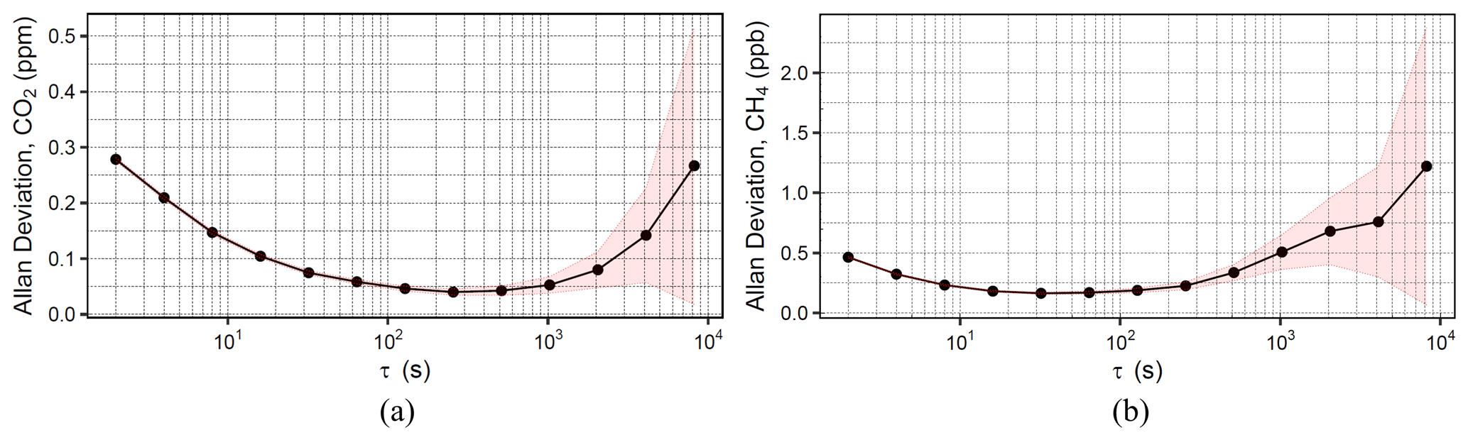
Figure 1 Allan deviation plots of (a) CO₂ and (b) CH₄. Here, τ is the sampling time in log scale, and the shaded region represents the 95 % confidence interval.

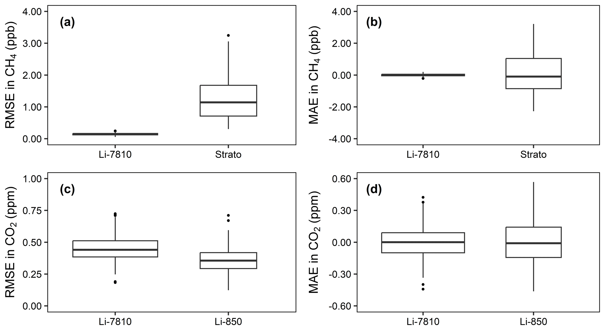
Figure 2 The 10 s averaged root mean square error (RMSE) and mean absolute error (MAE) of CH₄ (a, b) and of CO₂ (c, d), respectively. Here the interquartile range is shown as the rectangle box and the median as the horizontal bar within that box. Solid circles are the potential outliers, while the vertical lines represent the minimum and maximum values within the data.

2.2 Field site descriptions

The first field tests of the UAV platform were conducted over the Jena Experiment field site (50°57^′00^′′ N, 11°37^′30^′′ E), located north of Jena next to the Saale River in eastern Germany. The Jena Experiment has been the home of ongoing biodiversity research since 2002 (Weisser et al., 2017; Roscher et al., 2004). The core area of the experiment consists of several 20 m × 20 m vegetation patches and hosts 60 different plant species. The study area for our UAV campaigns at this site is fairly flat, covering approximately 400 m × 300 m, surrounded by trees along the edges. The average annual precipitation is 587 mm, and the mean annual air temperature is 9.3 °C (Roscher et al., 2004). To test our UAV system in a natural, heterogeneous ecosystem similar to our primary research target (i.e., the Arctic), we have conducted several flights over one of the most heavily investigated areas within the Arctic Circle, Stordalen Mire, a subarctic permafrost peatland in northern Sweden (68°21^′ N, 19°02^′ E), underlain by discontinuous permafrost (Bäckstrand et al., 2010) and showing a substantial small-scale heterogeneity in terms of soil moisture and vegetation types (Bäckstrand et al., 2010). The structure of this ecosystem offers a good opportunity to test the UAV platform's capability of detecting the impact of small-scale surface variability on GHG signals in the lower atmosphere. The average annual air temperature and precipitation are −0.6 °C and 304 mm, respectively (Malmer et al., 2005). The mire generally experiences two main wind directions (northwest–southeast) (see Fig. C1), and it is covered by snow between November and April, with a maximum depth of 55 cm (Malmer et al., 2005).

2.3 UAV platform characteristics and configuration

The UAV platform in our experiments is a hexacopter that can fly for about 20 min with a scientific payload of 4 kg (PM X6 Pro XL). The rotor–rotor distance is 1.29 m, and the propeller diameter (D) is 55.9 cm. CubePilot Cube Orange is used as a flight controller (Copter-4.4.2), equipped with triple heated internal measurement units (IMUs) and two barometers (https://docs.px4.io/main/en/flight_controller/cubepilot_cube_orange.html, last access: 11 April 2024). Integrated sensors of the flight controller, i.e., gyroscopes and accelerometers, log the motion of the UAV including roll, pitch, yaw, and accelerations in three-dimensional (3D) axes, which subsequently can be used to correct the wind speed measured by the anemometer. In addition to the GPS unit, a ground-pointing lidar is used to increase the vertical stability of the UAV.

Figure 3 Instrumented UAV platform (a) and close-up picture of the scientific payload (b).

Table 1 Characteristics of the scientific payload.

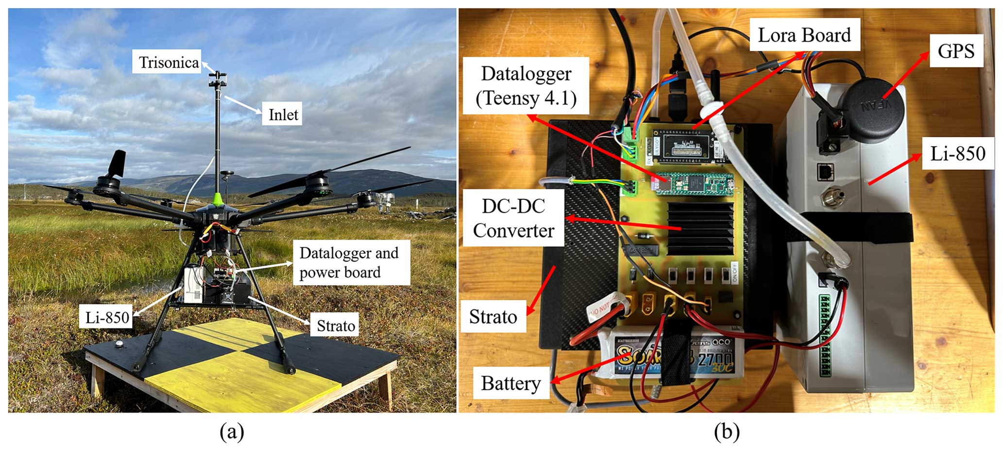
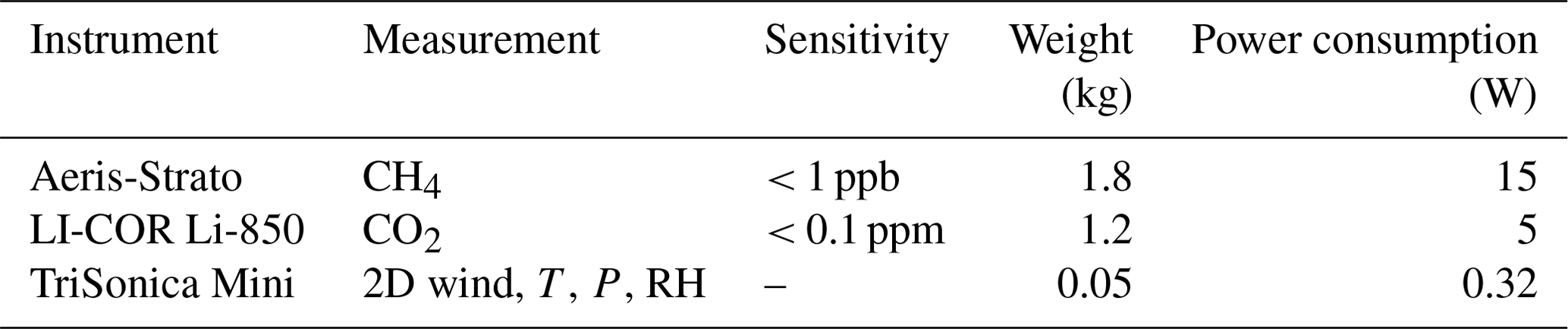
The scientific payload of this UAV platform (see Fig. 3a) includes a 2D anemometer (TriSonica Mini, LI-COR Environmental, USA) that measures the wind speed, air temperature, humidity, and pressure. The anemometer is placed 0.65 m above the rotor plane to avoid propeller downwash contaminating the anemometer measurement. This setup was previously found to provide satisfactory results (Palomaki et al., 2017; Shimura et al., 2018; Donnell et al., 2018; Thielicke et al., 2021; Bolek and Testik, 2022). However, measuring wind characteristics with an anemometer mounted on a UAV still remains a challenge, and compromises need to be made due to potential bias from the propellers and the flight stability. We decided to place the anemometer about 1.2 D above the rotor plane for the best system performance (the potential uncertainty sources and more information can be found in Yong et al., 2024). The platform is instrumented with two gas analyzers to measure CO₂ (LI-COR Li-850, LI-COR Environmental, USA) and CH₄ (Aeris Strato, Aeris Technologies) mole fractions, with both analyzers placed below the rotor planes. The internal pump of the LI-COR analyzer is removed to connect both analyzers sequentially, and the inlet of the tubing that leads sample air to both units is placed next to the anemometer. A custom-built data logger and power distribution board (see Fig. 3b) log onboard sensor data and provide power for the entire scientific payload. All data are synchronized at a frequency of 2 Hz, including secondary GPS data. Due to a frequency deviation issue (i.e., jitter) with the Strato analyzer, the collected data were slightly off from the intended 2 Hz (∼ 1.99 Hz). Therefore, we aggregated all data including UAV movement (translational and rotational motion data), gas analyzers, and anemometer data to 1 s during the data post-processing step. Additionally, the time lag associated with the inlet tubing length (about 1 s) was also compensated for in a post-processing step. Selected data (wind speed, wind direction, and GHG mole fractions) can be transferred to the ground control station using a LoRa (long-range radio communication) board, facilitating real-time data transmission while flying. Table 1 shows the specifications of the scientific payloads deployed on the UAV. The total take-off mass of the platform is 16.6 kg.

2.4 Data processing

Data collected by the UAV platform were pre-processed to correct or remove low-quality data related to sporadic spikes in CO₂ data. The TriSonica mini was set up to provide 3D wind information; however, the anemometer cannot resolve elevation angles higher than 15°. In addition, vertical wind speed is prone to biases due to disturbances caused by the propeller downwash. Therefore, we only used 2D wind speed for further analyses. The wind speed measured by the anemometer on the UAV platform was subject to disturbances due to translational and rotational (i.e., roll, pitch, and yaw) motion of the UAV. To compensate for these types of motion, we followed the direct correction methods, outlined by Donnell et al. (2018). Here, the heading of the UAV was kept constant during operation (i.e., no changes in yaw), and the anemometer north was aligned with the UAV's heading. Briefly, we first separated the 3D wind vector into components (u, v, and w) using wind speed (WS), direction (WD), and elevation angles. Similarly, the UAV's movement along 3D axes was also calculated from the measured GPS speed and yaw angles. To compensate for the rotational effects, the perturbations (r_θ, r_ψ) due to UAV motion were calculated as follows:

$$\begin{array}{}\text{(3)}& r_{\mathit{\theta }}=\left({\displaystyle \frac{{\mathit{\theta }}_i-{\mathit{\theta }}_{i-\mathrm{1}}}{\frac{\mathrm{1}}{f}}}\right)\times r\end{array}$$

$$\begin{array}{}\text{(4)}& r_{\mathit{\psi }}=\left({\displaystyle \frac{{\mathit{\psi }}_i-{\mathit{\psi }}_{i-\mathrm{1}}}{\frac{\mathrm{1}}{f}}}\right)\times r.\end{array}$$

Here, θ, and ψ represent roll and pitch, respectively; r is the distance between the rotor plane and the anemometer (65 cm); and f is the sampling frequency of the IMU of the UAV. The true wind speed was obtained from the raw wind speed (u_raw, v_raw, and w_raw) measured by the anemometer in combination with rotational and translational velocities (u_gps, v_gps, and w_gps) of the UAV, as shown in Eqs. (5) and (6) below. It should be noted that opposite sign conventions were adopted for the velocities of the anemometer and UAV.

$$\begin{array}{}\text{(5)}& {\displaystyle }\begin{array}{rl}u=& \left(u_{\mathrm{raw}}+r_{\mathit{\theta }}-u_{\mathrm{gps}}\right)\times \cos \left({\mathit{\theta }}_i\right)\\ & -(w_{\mathrm{raw}}+w_{\mathrm{gps}})\times \sin \left({\mathit{\theta }}_i\right)\end{array}\text{(6)}& {\displaystyle }\begin{array}{rl}v=& \left(v_{\mathrm{raw}}+r_{\mathit{\psi }}-v_{\mathrm{gps}}\right)\times \cos \left({\mathit{\psi }}_i\right)\\ & -(w_{\mathrm{raw}}+w_{\mathrm{gps}})\times \sin \left({\mathit{\psi }}_i\right)\end{array}\end{array}$$

Using the yaw angle of the UAV, we aligned the heading of the UAV to true north by rotating the coordinate system:

$$\begin{array}{}\text{(7)}& {\displaystyle }{u}_{\mathrm{rot}}=u\times \cos \left(\mathit{\alpha }\right)+v\times \sin \left(\mathit{\alpha }\right)\text{(8)}& {\displaystyle }{v}_{\mathrm{rot}}=-u\times \sin \left(\mathit{\alpha }\right)+v\times \cos \left(\mathit{\alpha }\right).\end{array}$$

Here, u_rot and v_rot are the rotated wind components and α is the difference between the UAV yaw angle and true north. Finally, 2D wind speed (WS) and true wind direction (WD) were calculated as

$$\begin{array}{}\text{(9)}& {\displaystyle }\mathrm{WS}=\sqrt{u_{\mathrm{rot}}^{\mathrm{2}}+v_{\mathrm{rot}}^{\mathrm{2}}}\text{(10)}& {\displaystyle }\mathrm{WD}=\mathrm{atan}\mathrm{2}(v_{\mathrm{rot}},u_{\mathrm{rot}}).\end{array}$$

To remove potential offsets in the calibration of the analyzers (see Sect. 2.1), we sampled high and low calibration gases with known CO₂ and CH₄ mole fractions (341.19 ± 0.01 and 543.1 ± 0.01 ppm and 1722.0 ± 0.1 and 2990.3 ± 0.1 ppb, respectively) before and after each flight day for about 2 to 5 min. These gas cylinders were calibrated following WMO calibration scales (WMO CO₂ X2019, WMO CH₄ X2014A) through a set of standards that were calibrated by NOAA (for more information, see Heimann et al., 2022). Note that only the last 1–2 min of sampling was used for the calibration process to allow the analyzer cells to be flushed for the first few minutes to reach the equilibrium. Observed offsets to the target mole fractions were compensated for during the data processing step using simple linear interpolation. Additionally, the CO₂ data were subject to filtering due to observed sporadic spikes during some flights. We first employed hard thresholds that omitted CO₂ mole fractions below 380 ppm and above 460 ppm, respectively. These plausibility limits were derived from long-term observations of the nearby ICOS tower CO₂ measurements. In addition, CO₂ data were omitted when the absolute difference between sequential CO₂ data was higher than 2 ppm or equal to zero. After eliminating implausible data this way, we applied the despiking algorithm from the RFlux package in R (Vitale et al., 2020) with the default scale parameter and 1 min window width. The despiking algorithm uses a repeated median filter within the selected window length to find the low-frequency part (μ_t) of the time series and replaces the detected spikes with μ_t (see Vitale, 2021 for further details).

2.5 Flight strategies

This study compiles data collected by our UAV platform over the Jena Experiment and Stordalen Mire, i.e., from a total of 40 independent flights and a combined flight time of about 12 h. Over these deployments, two distinct flight strategies were tested, namely grid surveys and vertical profile flight.

The grid survey flights were used to qualitatively assess the signal variability over the heterogeneous landscape of Stordalen Mire. Here, our UAV platform was programmed to fly at a constant speed following a pre-defined horizontal grid pattern. The grid surveys started with transects oriented along the east–west direction and were subsequently followed by north–south legs so that the same locations were sampled twice at two different times at transect intersections. The distance between each of these black circles is approximately 2 m based on the sampling frequency of 2 Hz and the flight speed of 4 m s⁻¹.

The vertical profile flights were conducted to observe vertical gradients of atmospheric conditions within the lowest part of the boundary layer and quantify the fluxes using the profile method, described in detail in the next subsection. These flights consisted of multiple waypoints along the z direction, at which the UAV platform was programmed to hover for 40 or 60 s depending on the pre-defined maximum altitude. The vertical resolution of the flight was set to 2.5 m up to a height of 15 m a.g.l., between 15 and 30 m a.g.l. it was 5 m, and from 30 to 110 m a.g.l. it was 10 m. The starting altitude of the vertical profile flights over the area was set to 5 m a.g.l.

2.6 Flux quantification using profile method

This section describes a quantification method (i.e., profile method) that was used to calculate the CO₂ and CH₄ fluxes based on vertical profile data. In essence, the approach is an application of the flux-gradient method (Xiao et al., 2014; Zhao et al., 2019; You et al., 2021) to UAV-based data. In the flux-gradient method, turbulent transport is comparable to molecular diffusion, allowing vertical fluxes to be approximated as the product of the vertical gradient of GHG mole fractions and the eddy diffusivity (Baldocchi et al., 1988). One of the main advantages of using the profile method in UAV-based calculations is the comparatively short required sampling time, since only mean values of the mole fractions are needed. Firstly, a logarithmic curve was fitted to the vertical mean wind profile as given in Eq. (11) (Foken, 2017; Tagesson, 2012):

$$\begin{array}{}\text{(11)}& \stackrel{\mathrm{‾}}{\mathrm{WS}\left(z\right)}={\displaystyle \frac{u_{*}}{\mathit{\kappa }}}\ln {\displaystyle \frac{z}{z_{\mathrm{0}}}},\end{array}$$

where κ is the von Karman constant [–] that is equal to 0.4, z is the measurement height [m a.g.l.], and z₀ is the roughness length [m]. Equation (11) can be rewritten as

$$\begin{array}{}\text{(12)}& \stackrel{\mathrm{‾}}{\mathrm{WS}\left(z\right)}=a\ln \left(z\right)+b,\end{array}$$

where a is the slope of the logarithmic curve fitting defined as $u_{*}/\mathit{\kappa }$, and b is the intercept. Based on Eq. (12), u_* [m s⁻¹] can be estimated using the slope of the logarithmic fittings to the wind speed profiles. Under the assumption of neutral stability and estimation of u_*, the eddy diffusivity (K_ed) can be derived as given in Eq. (13) (Zhao et al., 2019):

$$\begin{array}{}\text{(13)}& K_{\mathrm{ed}}=\mathit{\kappa }{u}_{*}{z}_{\mathrm{g}},\end{array}$$

where z_g is the geometric mean of the two altitudes (z₁ and z₂) between which the flux is being considered. To calculate K_ed and the fluxes, we used the lowest two altitudes of our UAV-based vertical profile measurements (i.e., z₁=5 and z₂=7.5 m). The reason for this is that near the surface, fluxes are only expected to be influenced by local emissions (i.e., smaller footprint area), while at higher altitudes signals from different sources and sinks over the landscape may affect the measurements (i.e., larger footprint area), complicating the interpretation of the results. Using K_ed, the fluxes (F) of CO₂ and CH₄ can be estimated as given in Eq. (14) (You et al., 2021).

$$\begin{array}{}\text{(14)}& {\displaystyle }F=-K_{\mathrm{ed}}{\displaystyle \frac{{\mathit{\chi }}_{\mathrm{1}}-{\mathit{\chi }}_{\mathrm{2}}}{z_{\mathrm{1}}-z_{\mathrm{2}}}}\text{(15)}& {\displaystyle }\mathit{\chi }={\displaystyle \frac{\stackrel{\mathrm{‾}}{P}M\stackrel{\mathrm{‾}}{C}}{R\stackrel{\mathrm{‾}}{T}}}\end{array}$$

In Eq. (15), χ₁ and χ₂ are the measured mass concentrations of CO₂ [g CO₂] or CH₄ [g CH₄], respectively, at 5 and 7.5 m (Gålfalk et al., 2021). Here, $\stackrel{\mathrm{‾}}{P}$ is the average pressure [Pa], $\stackrel{\mathrm{‾}}{C}$ is the measured averaged mole fractions of CO₂ or CH₄ at each altitude [ppm], M is the molar mass [g mol⁻¹] with 44.01 for CO₂ and 16.03 for CH₄, R is the universal gas constant equal to 8.314 [J K⁻¹ mol⁻¹], and $\stackrel{\mathrm{‾}}{T}$ is the averaged temperature [K]. The negative sign is introduced as a convention, so positive fluxes are emissions from the ecosystem to the atmosphere, and negative fluxes signify uptake. The uncertainties of the flux calculations and friction velocity estimations were derived using Monte Carlo simulations with a probability level of the coverage interval of 0.95 (i.e., Monte Carlo trials of 20 000) (Veen and Cox, 2021). To perform the Monte Carlo simulations, we first generated normally distributed synthetic data for wind speed and mass concentrations of CH₄ and CO₂ based on the measured means and standard deviations at each altitude. These generated synthetic data were then used to estimate the uncertainties of the friction velocities as well as the fluxes of CO₂ ($F_{{\mathrm{CO}}_{\mathrm{2}}}$) and CH₄ ($F_{{\mathrm{CH}}_{\mathrm{4}}}$) (for more details, please see Veen and Cox, 2021).

3 Results and discussion

3.1 Flights over the Jena Experiment

Over the Jena Experiment site, we conducted test flights to evaluate the instruments within our scientific payload against tower-based eddy covariance reference measurements. For these test flights, a different calibration gas sampling procedure compared to the one explained in Sect. 2.4 was applied. The field experiment was conducted on 14 July 2023, and the data were compared with observations from a 2 m high local tower, which was placed temporarily, instrumented with a 2D anemometer and a LI-COR Li-850 analyzer.

Figure 4 shows the comparison of wind speed, CO₂, and H₂O concentrations between UAV and tower datasets. The flight lasted about 21 min, and the UAV was hovering at 10 m high above the ground level during the entire flight. The reason for not hovering closer to the ground, ideally the same height as the tower, is the surrounding trees and fences near the tower location which prevent safe UAV flights from being conducted at lower altitudes. As there was no additional stationary CH₄ analyzer, the comparison does not include CH₄. A calibration gas mixture was sampled from a gas cylinder to quantify the offset between the CO₂ analyzers after the flight; no calibrations were performed beforehand. The tank was sampled for 14 min, and the average offset was corrected for in the subsequent analyses. Overall, good agreement between UAV and tower was observed, with a correlation coefficient (r) higher than 0.6 for all measured variables. During the flight, the mean difference between the CO₂ concentrations was 3.34 ± 0.91 ppm. A large fraction of this difference can be attributed to vertical concentration gradients within the atmospheric boundary layer (see, e.g., reference vertical profiles between 2.5 and 10 m from the meteorological tower of the Lindenberg observatory in Germany in Fig. B1). Another factor influencing the comparison of CO₂ signals is that CO₂ mixing ratios were not converted to dry-air mole fractions here for both tower- and UAV-based gas analyzers. It should be noted that in the rest of this paper, CO₂ mixing ratios are reported as dry-air mole fractions. Due to the short measurement time, fluctuations of atmospheric moisture can be neglected, but vertical gradients in H₂O levels may lead to minor absolute offsets between signals from both analyzers. Furthermore, the fact that the local tower is below the canopy height (due to technical limitations) might also affect the observed gradient. For the wind speed comparison between the tower and the UAV, we found a high correlation coefficient of 0.639, even though the wind speed correction procedure could not be performed due to the lack of elevation angle data in the data logger. The highest correlation between the tower and the UAV (r=0.709) was observed for the H₂O measurements.

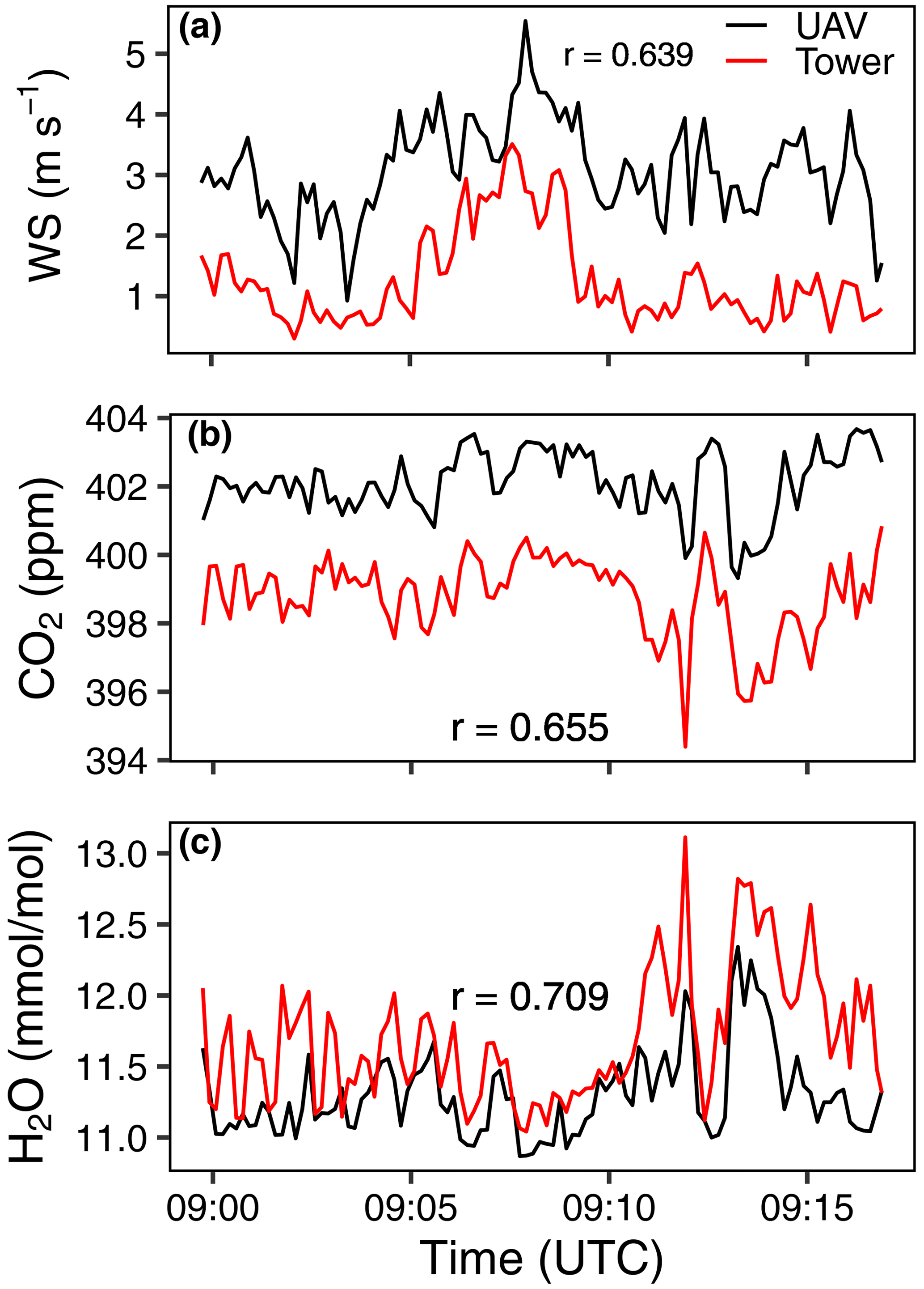
Figure 4 The 10 s averaged time series of (a) wind speed, (b) CO₂, and (c) H₂O illustrated by the black line for UAV and the red line for tower measurements. Here, r represents the correlation coefficient between the tower and the UAV.

3.2 Grid flights over Stordalen Mire

Several grid survey flights were conducted over Stordalen Mire in the period 11 to 14 September 2023, with the main focus to identify potential hot spots in atmospheric GHG mole fractions and quantify the signal variations over the areas of interest. Three different target areas were defined using the vegetation map from Varner et al. (2022): two of them, labeled as Area 1 and Area 2 in the following, were classified as bog and fen, respectively, and thus featured mostly wet surfaces. The third domain, Area 3, was mostly dry and was classified as a palsa mire (see Fig. 5). Each of these areas was surveyed two times. All grid survey flights were conducted at an altitude of 10 m a.g.l., and each flight lasted about 14 min. Sampling within each grid survey was interrupted for about 15 to 20 min to prepare the UAV platform for the second flight leg. The only exception to this was the second survey over Area 3, for which, due to bad weather conditions, the second part of the survey needed to be postponed to the following day (see also details of the grid survey flights in Table 2). All survey grid data were subject to a filtering process to remove observed sporadic spikes in CO₂ data, as was described in Sect. 2.4.

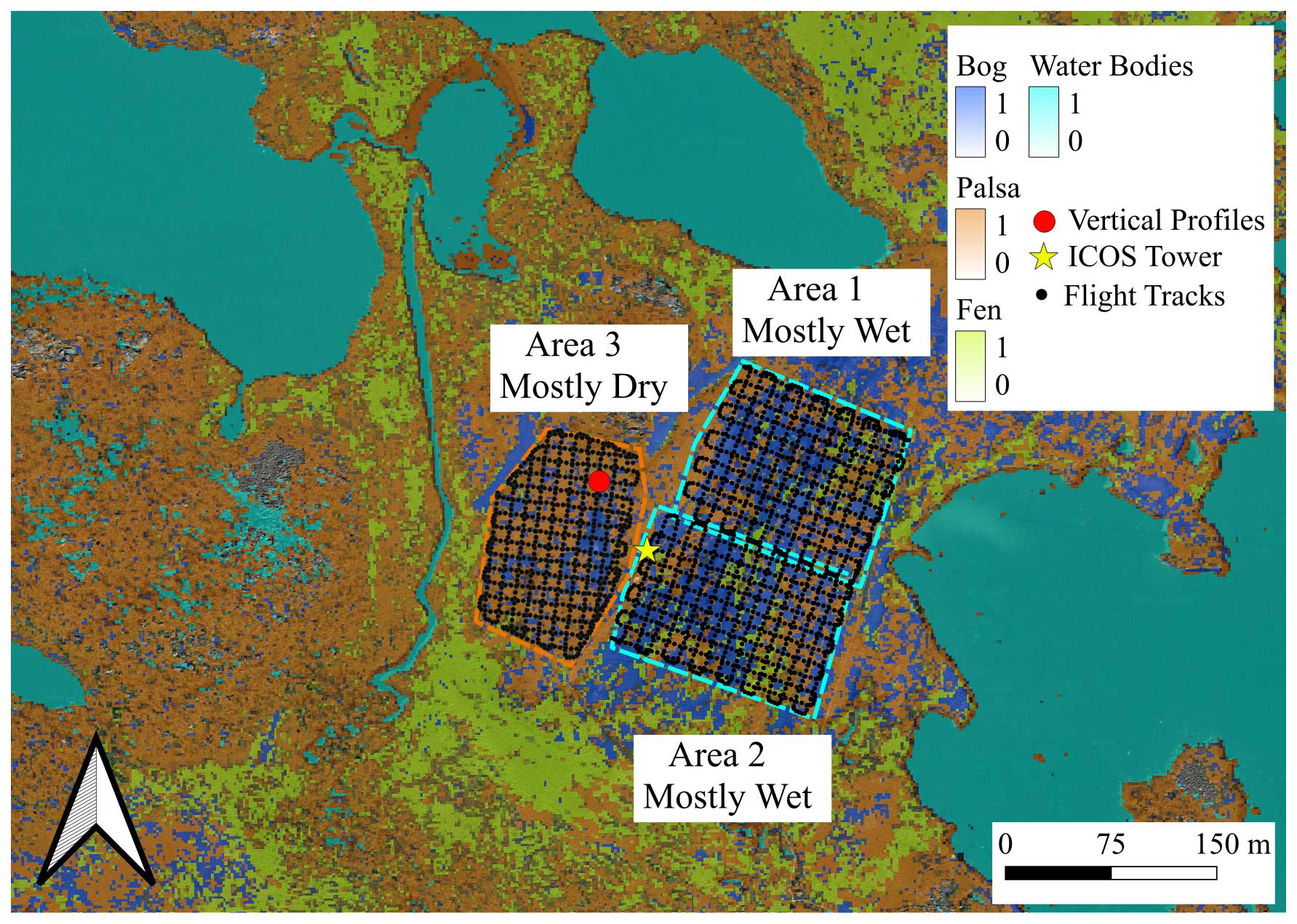
Figure 5 Overview of conducted flights in Stordalen. Flight tracks of grid surveys over three different areas. Here, the land cover map (Varner et al., 2022) shows the vegetation distribution, and the border of areas was represented by dashed lines (blue for wet, orange for dry). Flight tracks are indicated with solid black circles. The location of the vertical profiles was illustrated with a red circle, whereas the location of the ICOS tower was depicted with a star.

Table 2 Flight details over Stordalen Mire.

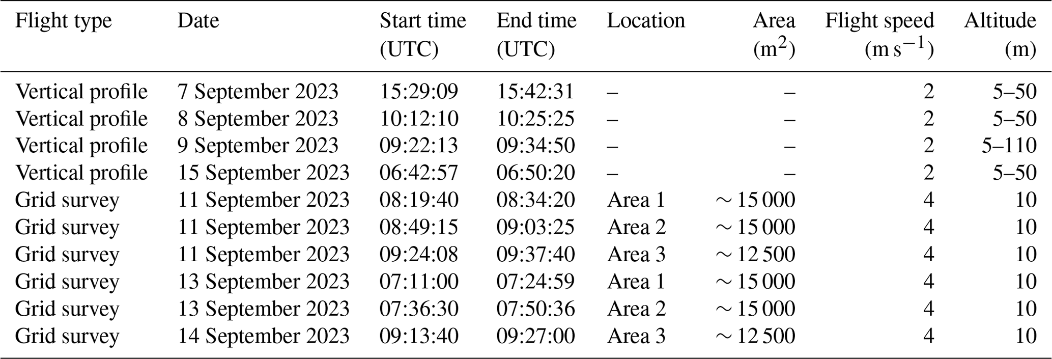
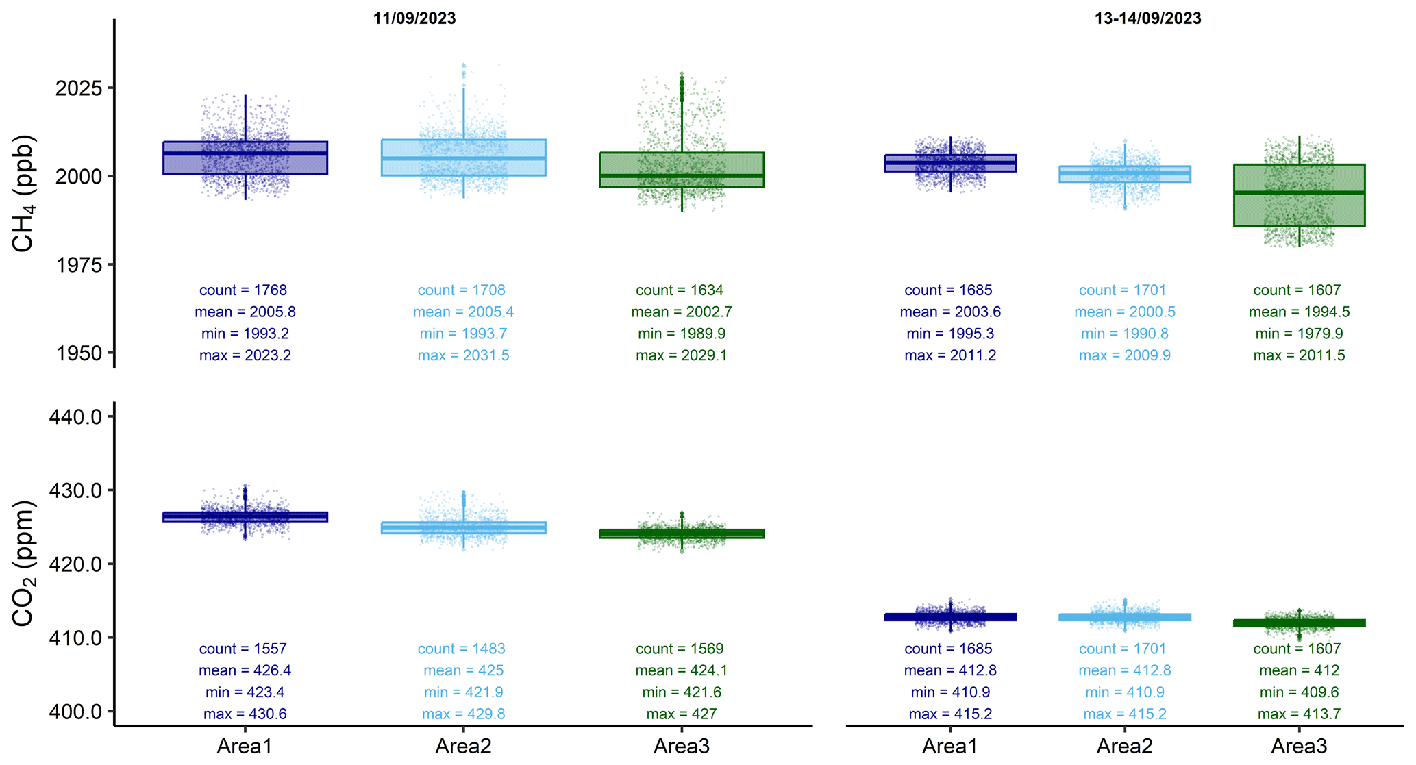
Figure 6 CH₄ and CO₂ mole fractions measured by UAV from the grid survey flights on 11 and 13–14 September 2023. The measured data points (2 Hz) are shown, and the outliers are represented as diamonds. Basic statistics including the number of data points as count and the mean, min, and max values are denoted underneath each corresponding box plot.

The mole fractions of CH₄ over Areas 1 and 2 were found to be higher than those over Area 3 for both flight days (see Fig. 6). This could most likely be attributed to higher methane emissions, indirectly corroborated by higher water availability, previously identified as one of the main drivers of CH₄ emissions (Kwon et al., 2022). From the land cover map used within this study (Fig. 5), we estimated that about 70 %–75 % of both Area 1 and Area 2 was either bog or fen, while the fraction of these classes was estimated at only about 30 % for Area 3. Furthermore, we found the variability of the measured CH₄ mole fractions to be highest over Area 3 (average 35.4 ppb), compared to an average of 22.9 and 28.5 ppb for Area 1 and Area 2, respectively (see Fig. 6).

Opposed to our findings, Scheller et al. (2022) found smaller variability of CH₄ over dry tundra compared to fen areas. This might be due to the different measurement heights of the two studies: here the measurement height was 10 m, while in Scheller et al. (2022) it was about 0.3 m. Additionally, although Area 3 was specified as mostly dry, it still comprises small patches of fens and bogs. Since the measurements over Area 3 were conducted on a different date than those for Areas 1 and 2, the observed variations may also be linked to different environmental conditions; however, the measured CO₂ mole fractions were also higher over Areas 1 and 2 compared to Area 3. Furthermore, the variations of CO₂ over Areas 1 and 2 were found to be about 6 ppm, whereas the variation was about 4.8 ppm over Area 3. Overall, our UAV-based observations over Stordalen Mire demonstrate that the spatial variability in CO₂ and CH₄ mole fractions can be high, even over small spatial scales. This implies that measurements made by stationary EC towers may be subject to substantial location biases in complex environments such as Arctic wetlands.

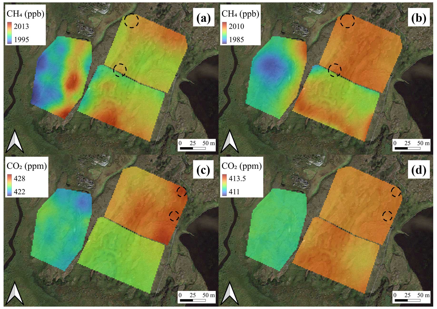
Figure 7 Interpolated CH₄ and CO₂ mole fractions (overlaid on satellite image from © Google Maps), using the Kriging algorithm of the grid surveys that were conducted on 11 September 2023 (a, c) and on 13–14 September 2023 (b, d). Note that legends are different for each measurement day to highlight the potential hot spots. Here, color gradients from blue to red were used where blue colors represent low, and red colors represent high mole fractions. Potential hot spots were enclosed by dashed black lines.

The grid survey data were spatially averaged into 10 grid cells, each in a latitude and longitude direction, which resulted in a grid with a spatial resolution of about 15–20 m. Bins with fewer than 20 data points were excluded from further analysis. We then interpolated the spatially averaged data using the ordinary Kriging algorithm (Pereira et al., 2022) to facilitate a visual overview of the mole fraction distribution over the study areas (see Fig. 7). In this context, best-fitted model variograms were selected based on the RMSE and coefficient of determination (R²). Using interpolated maps, potential hot spots could be identified. Respective areas are enclosed by dashed black lines in Fig. 7. Potential hot spot areas were identified by first locating the 95 percentile of mole fractions over each flight area and flight day; subsequently the locations with matching hot spots for both survey days were identified on the map. Overall, the gridded datasets showed a range in CH₄ mole fractions of up to 25 ppb for a single measurement period across the three target sites, while this range was 6 ppm for CO₂ mole fractions. Considering the rather small size of the study domain, this level of variability emphasizes the heterogeneity of ecosystem characteristics and corresponding carbon cycle processes within structured wetlands and highlights the value of survey flight data as presented within this study.

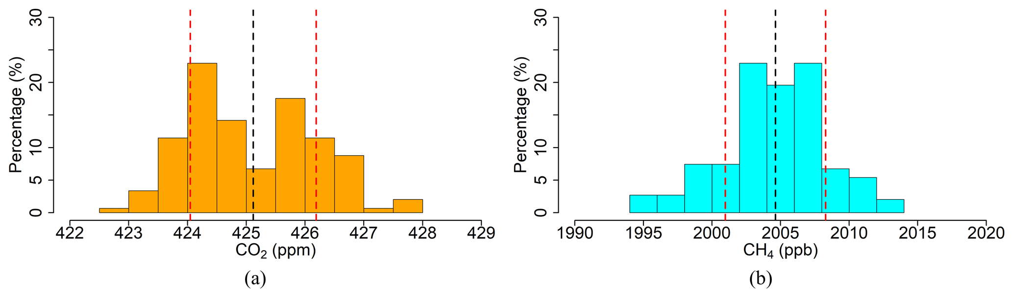
Figure 8 The distribution of spatially averaged CO₂ (a) and CH₄ (b) mole fractions of all three areas combined. The black dashed lines are the corresponding averages, while the red dashed lines are the ±σ, where σ is the standard deviation.

Over Area 3, the eastern part of the domain showed particularly high CH₄ mole fractions on both days. These areas are close to Areas 1 and 2, and it is therefore possible that a signal that originated in either Area 1 or Area 2 might be picked up by the UAV platform while flying over Area 3 due to horizontal advection. At the same time, enhanced CH₄ may also be correlated with the distribution of wet microsites within Area 3. Spatial variability within the CH₄ and CO₂ mole fraction fields at such small scales, as shown in these horizontal maps, is very challenging to detect with conventional stationary measuring methods. The frequency distribution of observed mole fractions within all three areas is illustrated in Fig. 8. Here, only data from the 11 September 2023 flights were selected, since all areas were sampled within the same day. The means of the mole fractions were 425.12 ppm for CO₂ and 2004.62 ppb for CH₄, with standard deviations of 1.07 ppm and 3.66 ppb, respectively. Figure 8 emphasizes that the mole fractions over the significant section of the total area (about 35 % and 26 % of CO₂ and CH₄, respectively) do not overlap with the designated threshold (i.e., μ±σ, where μ is the mean, and σ is the standard deviation), which again highlights the pronounced signal variability over heterogeneous landscapes. Therefore, we recommend combining maps like these ones with eddy tower and chamber data to improve the interpretation of observational studies over complex ecosystems and to minimize potential representativeness errors which would, e.g., affect modeling frameworks that are trained with such datasets.

3.3 Vertical profile flights over Stordalen Mire

Apart from the grid survey flights, vertical profile flights were conducted between 7–9 and 15 September 2023, covering elevations of up to 110 m above the ground level (see Table 2). Only the ascending profile was used in our analysis to avoid sampling an air column disturbed by the rotor downwash. The lowest part of the boundary layer profile was created by averaging every 10 s aggregated block at each altitude (see Fig. 9). The two main wind directions (northwest–southeast) (see Fig. C1) also captured with the vertical profiles were east-southeast (8 and 15 September) and west-northwest (7 and 9 September). CO₂ mole fractions mostly show a well-mixed behavior, except for the profile observed on 8 September, where lower CO₂ mole fractions are observed at the mid-altitudes, between approximately 15 and 35 m. Measured vertical profiles presented here are likely affected by an internal boundary layer (IBL), since the area is surrounded by lakes where the surface roughness is small compared to the heterogeneous surfaces around the measurement point, and energy fluxes likely carry different signatures. The formation of the IBL is evident on the profile of 8 September, where the most likely explanation of the observed profile is that the airflow first crossed the entire lake on the eastern side and was subsequently affected by the heterogeneous surface between the lake coast and the measurement location. In our vertical profile, the associated transition layer forms above 15 m a.g.l., where the wind speed decelerates due to a smooth–rough transition demonstrated, similar to Krishnamurthy et al. (2023). CH₄ mole fractions show high variations for all the profiles and generally are complex to interpret. Nevertheless, higher CH₄ enhancement is observed under easterly wind as opposed to westerly wind. Although day-to-day variations might also play an important role, from the land cover map it is clear that the eastern side of the profile measurement point comprises a higher number of wet areas suspected to be the source of CH₄. The lowest CH₄ mole fractions were recorded on the 7 September profile, where the wind direction was 268.8 ± 21.6° (i.e., westerly wind), while higher mole fractions were observed when the wind direction was 108.6 ± 14.4 and 147.8 ± 3.1° (east-southeast) on the 8 and 15 September profiles, respectively. The profile on 9 September is more complex to interpret since the landscape changes back and forth from lake to land on the northwest side of the measurement point. Considering the profile on 8 September where an IBL formation was inferred, the CH₄ profile seems to also be affected by the IBL. The mid-altitudes have the highest CH₄ mole fractions where the signals might be originating from the area between the measurement point and the lake on the eastern end from the land cover map (see Fig. 5), which is dominated by fen or bogs. CH₄ mole fractions decrease at higher altitudes (above the IBL) where the signal might be forming over the lake.

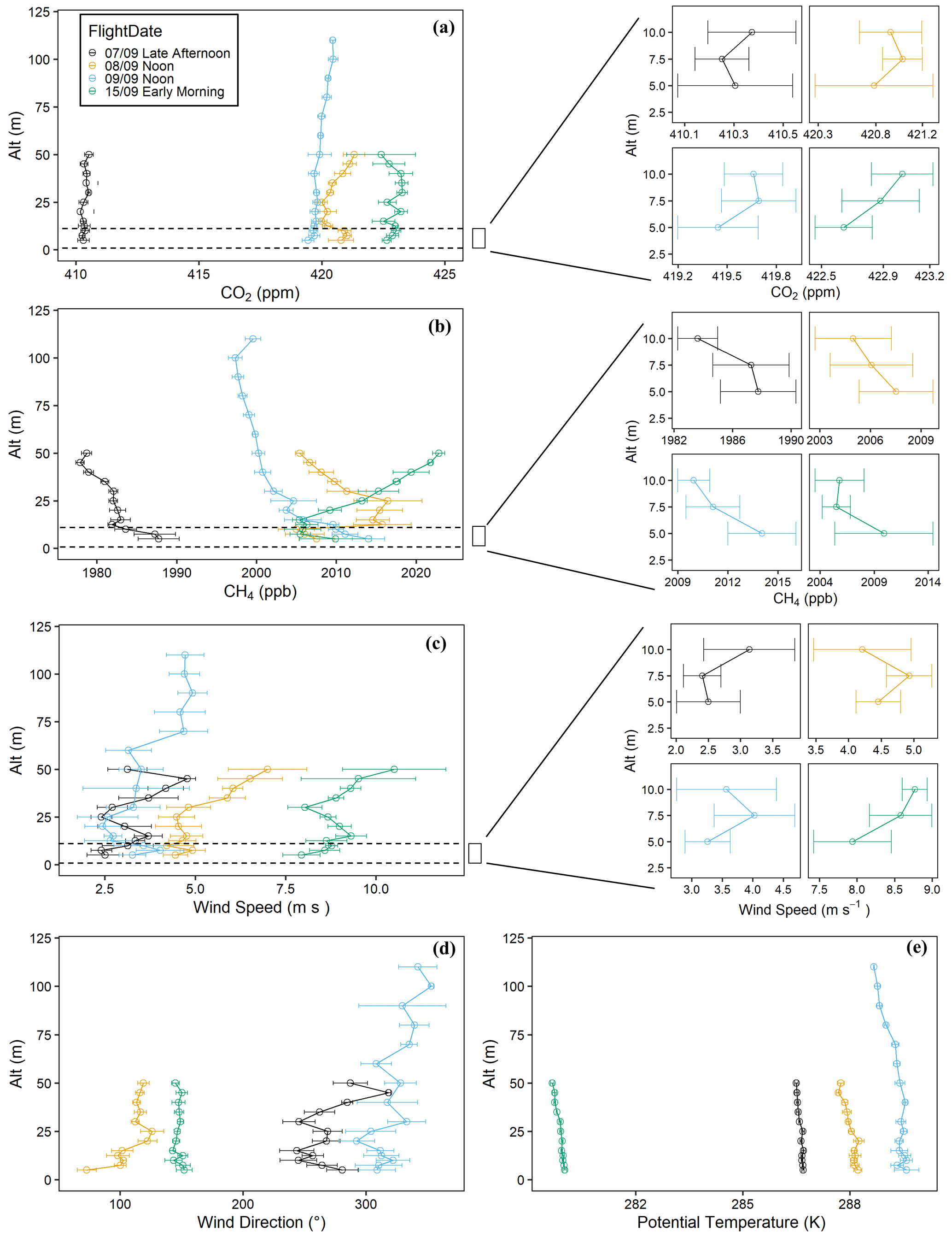
Figure 9 Vertical profiles of (a) CO₂, (b) CH₄, (c) wind speed, (d) wind direction, and (e) potential temperatures. Here each symbol represents the average of each 10 s block, and horizontal lines represent the standard deviations. Profiles of wind speed, CH₄, and CO₂ close to the surface (z ≤ 10 m) were provided as a close-up view next to the corresponding figures.

Table 3 Estimated friction velocities (u_*) and fluxes of CH₄ ($F_{{\mathrm{CH}}_{\mathrm{4}}}$) and CO₂ ($F_{{\mathrm{CO}}_{\mathrm{2}}}$) from the vertical profiles and corresponding uncertainties. Reference values (_Twr) were derived using observations from the ICOS EC tower at Stordalen Mire.

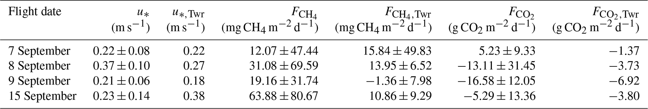
The quantification method as explained in Sect. 2.6 was applied here for all vertical profiles to constrain $F_{{\mathrm{CH}}_{\mathrm{4}}}$ and $F_{{\mathrm{CO}}_{\mathrm{2}}}$ (see Table 3). All conducted flights show CH₄ emissions, and the average emissions when the wind was blowing from the east side of the measurement location (47.48 ± 75.13 mg CH₄ m⁻² d⁻¹) was found to be higher compared to those from the westerly directions (15.62 ± 39.59 mg CH₄ m⁻² d⁻¹). Higher CH₄ fluxes were also observed at the eastern side of the ICOS EC tower, compared to the western side (Łakomiec et al., 2021), supporting our UAV-based observations. On the other hand, except for the 7 September flight, all the flights show CO₂ uptake over the measuring location. Observed CO₂ emissions on 7 September might be due to lower incoming shortwave radiation since the measurement was conducted in the late afternoon (around 17:30 local time). As a rough validation, we used ICOS EC tower data (SE-Sto) to calculate the $F_{{\mathrm{CH}}_{\mathrm{4}},\mathrm{Twr}}$ using the EC method due to the lack of $F_{{\mathrm{CH}}_{\mathrm{4}}}$ data on the ICOS Portal. However, for the $F_{{\mathrm{CO}}_{\mathrm{2}},\mathrm{Twr}}$ fluxes and $u_{*,\mathrm{Twr}}$, data from the ICOS Portal were used (Lundin et al., 2024). Here, the calculations were done as closely as possible to the sampling times of the vertical profiles using a 30 min averaging time. For the profiles of 7 and 9 September, mean fluxes for a full hour are used, since the flight took place in the middle of two 30 min datasets. Furthermore, the uncertainties of the tower-based $F_{{\mathrm{CH}}_{\mathrm{4}}}$ were calculated following Mann and Lenschow (1994). Note that the $F_{{\mathrm{CH}}_{\mathrm{4}}}$ calculations here may lead to enhanced uncertainties since limited data quality information was available. Still, this preliminary comparison with the EC tower shows acceptable qualitative agreement considering footprint differences between the UAV and ICOS EC tower, which are affected by the spatial variability of the fluxes and the difference in measurement heights (i.e., the effective measurement height of the UAV-based calculations is z_g, which is 6.12 m, whereas for ICOS EC tower it is 2.2 m). Although logarithmic fittings that were used to estimate the friction velocities are not perfect (average R² values were around 0.31, 0.57, 0.38, and 0.4 for 7, 8, 9, and 15 September, respectively), estimates were in an acceptable range since at least 12 altitude levels were used to represent the vertical profiles, and the variations can mostly be attributed to the deviations in the stability conditions from the neutral case. The relatively high uncertainties of the calculated fluxes (see also Table 3) are, to a large extent, due to the small vertical gradient of CO₂ and CH₄ relative to the combination of background signal variations and instrument drift. This can be seen, e.g., from the panels in Fig. 9, where only the profile part z≤10 m of the boundary layer was illustrated. In most cases observed in this study, the deviations in the signal are higher than the vertical gradient. Here, the assumption of neutral stability and logarithmic profile might also contribute to the observed high uncertainties. In principle, it would be better to select altitudes with a larger mole fraction difference in order to get a better-defined gradient (Tagesson, 2012), but since the vertical profiles are affected by IBL formation, we avoided using higher altitudes. Ideally, setting the lowermost measurement altitude a bit closer to the ground at about 2–3 m and the second at around 10 m would be preferable. Also, the measurements were conducted during the late growing season when the fluxes are expected to be small. As a consequence, even though this method for UAV-based quantification of local-scale flux rates is promising, further research will be needed to reduce the uncertainties, e.g., using different quantification methods and optimized flight strategies.

4 Conclusions

In this study, we presented a state-of-the-art UAV platform instrumented with in situ CH₄ and CO₂ gas analyzers and an ultrasonic anemometer capable of measuring 2D wind speed, air temperature, humidity, and pressure. The observational material presented demonstrated how such UAV platforms can be used to collect both qualitative and quantitative information to interpret GHG exchange processes over complex natural terrain.

Two different flight strategies were tested in this study to sample the lowest part of the boundary layer over areas that are otherwise challenging to characterize with stationary devices. Grid survey flights were used to qualitatively represent spatial variability in GHG signals as well as to identify hot spots of the emission sources over a selected study area. Vertical profiles, in turn, were found to be particularly useful for specifying the characteristics within the lower atmospheric boundary layer, filling an important data gap that exists over the Arctic (and other remote areas), primarily due to logistical challenges. Additionally, we have shown that profile flights can be used to quantify the GHG fluxes directly using the profile method, though the data analyzed in the scope of this study showed that this approach is subject to large uncertainties and needs further research aimed at their reduction, potentially by employing different flight strategies. As a future profiling strategy, UAV ascending speed will be reduced, and the measurements above 25 m a.g.l. will be omitted to avoid the footprint contamination. In addition, the starting altitude of the profile flight should be closer to the ground, ideally around 2–3 m a.g.l. This will allow us to have multiple profiles within one flight set and help to reduce the uncertainties.

For future studies with the presented UAV platform, combining the grid survey flights with measured wind characteristics via explicit footprint analysis may help to improve the attribution of emission sources. Better localization of the emission hot spots on the surface will allow for improved upscaling of CH₄ and CO₂, especially if supplemented by stationary EC tower and chamber measurements. In the future, the method can also be applied over larger areas, allowing further closure of the scaling gaps, e.g., between local observations and satellite remote sensing at regional scales.

In summary, our study shows that UAV platforms are capable of providing valuable information on spatially variable greenhouse gas patterns within the atmospheric boundary layer, which can improve our understanding of greenhouse gas processes within complex landscapes. We have demonstrated the applicability of different flight strategies that can be used to support measurements from an existing carbon flux monitoring network, e.g., to assess signal representativeness of the upscaling. However, more flight strategies and quantification methods need to be tested to fully exploit the potential of UAV-based GHG observations for ecological research. This might also be accomplished by conducting synthetic UAV flights within a numerical model.

Appendix A

The time series of two gas analyzers sampling a calibration mixture are shown in Fig. A1. Here, the linear drift of the Li-850 can be seen, which within 21 min of flight time the drift is expected to be no more than 0.18 ppm. The Aeris Strato, on the other hand, shows non-linear drifts with a magnitude of no more than 4 ppb over the same period. Apart from the non-linear fluctuations, the drift is usually much less than 4 ppb. These drifts can most likely be attributed to a compromise in temperature stabilization, where the cell enclosure was stripped down in this instrument model to arrive at a sensor weight compatible with UAV application.

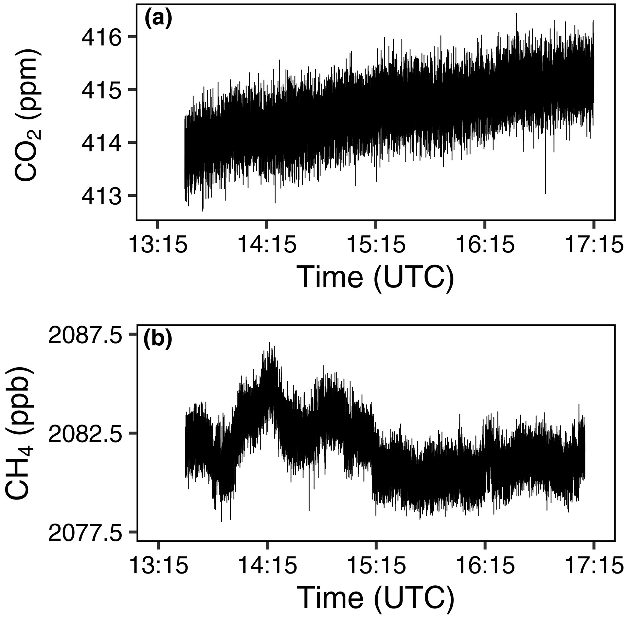
Figure A1 Sampling gas analyzers using calibration gas tanks with ambient air mole fractions: (a) LI-COR Li-850 and (b) Aeris Strato.

Appendix B

A box plot with CO₂ concentration differences between measurement heights at 2.5 and 10 m a.g.l. from Lindenberg tower is shown in Fig. B1. The Lindenberg tower is part of the Integrated Carbon Observation System (ICOS) network that provides accurate atmospheric measurements across Europe (ICOS RI et al., 2024). The gradient of the hourly CO₂ concentrations between 2.5 and 10 m above the ground level was found to fluctuate between −1.19 and 1.73 ppm at this site (see Fig. B1). Here, only summertime measurements (June to August) during the late morning hours (10:00–12:00 UTC​​​​​​​) within the period 2016 to 2022 were considered.

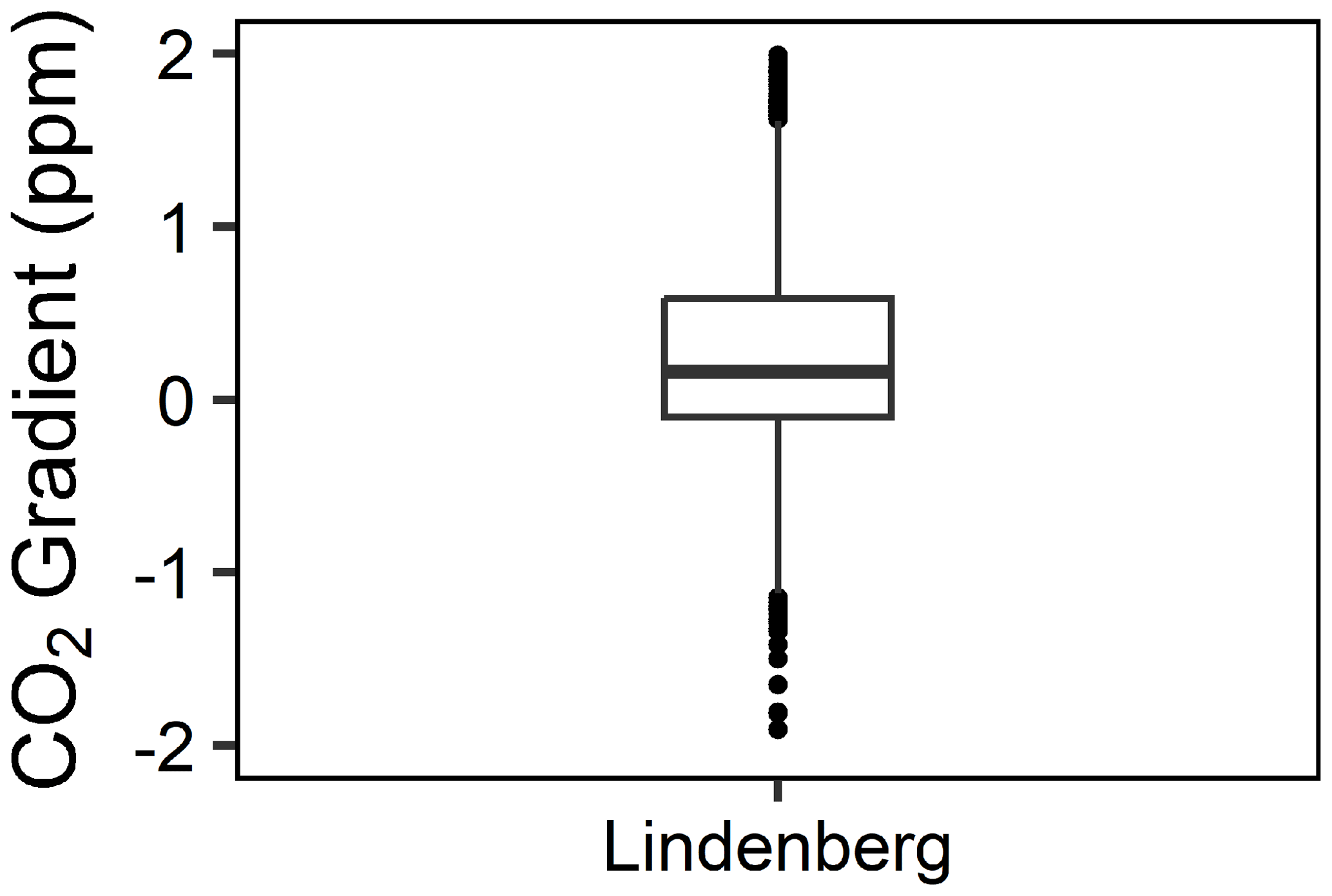
Figure B1 Gradient of CO₂ calculated from Lindenberg tower. Two measurement heights of 2.5 and 10 m were used here.

Appendix C

Wind characteristics over the Stordalen Mire (ICOS station ID: SE-Sto) were illustrated using 30 min averaged data between 31 December 2021 and 31 August 2023 (see Fig. C1). This 3-year record shows a clear domination of wind sectors in the WNW and ESE directions, respectively.

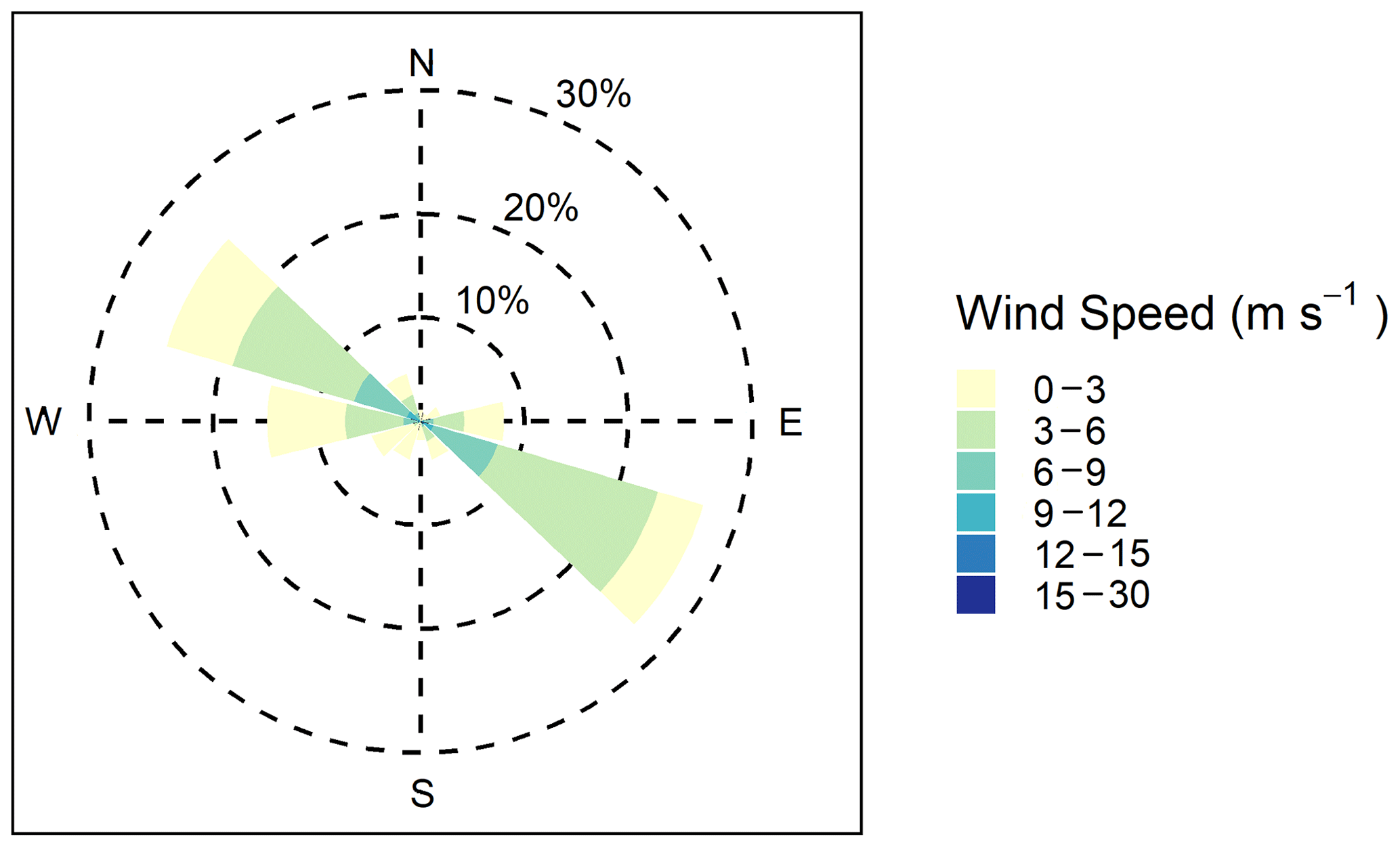
Figure C1 The wind rose as measured by the ICOS station located in Stordalen Mire, reflecting mean wind conditions between 31 December 2021 and 31 August 2023.

Appendix D

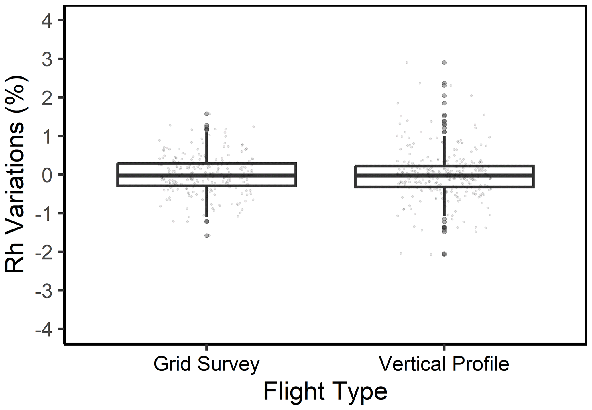
The variations in 10 s averaged relative humidity, after removing mean values of each individual flights, are shown in Fig. D1 for all flights listed in Table 2, except the grid survey flight over Area 3 on 11 September 2023. Due to a technical issue in anemometer, we do not have any humidity data from that flight. Overall, most of the data (about 95 %), regardless of flight type, vary within a ±1.5 % range.

Figure D1 The variations in 10 s averaged relative humidity for the flights listed in Table 2. Here, mean values of each flights were removed, and relative humidity data were grouped based on flight type, i.e., grid survey and vertical profile.