Marine cloud base height retrieval from MODIS cloud properties using machine learning

Clouds are a crucial regulator in the Earth's energy budget through their radiative properties, both at the top of the atmosphere and at the surface; hence, determining key factors like their vertical extent is of essential interest. While the cloud top height is commonly retrieved by satellites, the cloud base height is difficult to estimate from satellite remote sensing data. Here, we present a novel method called ORABase (Ordinal Regression Auto-encoding of cloud Base), leveraging spatially resolved cloud properties from the Moderate Resolution Imaging Spectroradiometer (MODIS) instrument to retrieve the cloud base height over marine areas. A machine learning model is built with two components to facilitate the cloud base height retrieval: the first component is an auto-encoder designed to learn a representation of the data cubes of cloud properties and to reduce their dimensionality. The second component is developed for predicting the cloud base using ground-based ceilometer observations from the lower-dimensional encodings generated by the aforementioned auto-encoder. The method is then evaluated based on a collection of collocated surface ceilometer observations and retrievals from the CALIOP satellite lidar. The statistical model performs similarly on both datasets and performs notably well on the test set of ceilometer cloud bases, where it exhibits accurate predictions, particularly for lower cloud bases, and a narrow distribution of the absolute error, namely 379 and 328 m for the mean absolute error and the standard deviation of the absolute error, respectively. Furthermore, cloud base height predictions are generated for an entire year over the ocean, and global mean aggregates are also presented, providing insights into global cloud base height distributions and offering a valuable dataset for extensive studies requiring global cloud base height retrievals. The global cloud base height dataset and the presented models constituting ORABase are available from Zenodo (Lenhardt et al., 2024).

1 Introduction

Clouds play a key role in the Earth's energy budget through their interactions with incoming shortwave and outgoing longwave radiation fluxes. It is thus critical to adequately quantify cloud radiative properties and their changes under global climate change. However, cloud radiative properties remain a large uncertainty in estimating anthropogenic climate change and possible impacts in the future (Boucher et al., 2013; Forster et al., 2021). Radiative properties of clouds are related to numerous quantities that can be used to characterise them. For instance, the cloud base height (CBH) is a crucial radiative property due to its impact on the surface longwave radiation. Furthermore, the cloud geometrical thickness (CGT), defined as the difference between the cloud top height (CTH) and the CBH, links to the adiabatic cloud water content, allowing the quantification of the cloud's subadiabaticity. Additionally, deriving the CBH is of practical use for pilots, providing crucial information during flights.

However, while the CTH can be rather easily obtained through passive satellite observations, the CBH retrieval remains problematic due to the fact that it is only indirectly accessible to satellites and due to retrieval errors related to satellite remote sensing, such as instrument shortcomings or noisy measurements. Since the difference between the CTH and the CBH quantifies the vertical extent of a cloud, one way to retrieve the CBH from passive satellites is by making heavy assumptions about the vertical distribution of the cloud water path inside the cloud profile. It is thus a challenging retrieval with passive satellite data that provide information about the cloud top (e.g. cloud top temperature (CTT), pressure (CTP), or height (CTH)) or about the entire column (e.g. cloud optical thickness (COT)) assuming the cloud's adiabaticity. For example, Noh et al. (2017) rely on a semiempirical approach to link the CGT to the CTH and the cloud water path (CWP – includes both ice and liquid water paths). In a different approach, Böhm et al. (2019) retrieve the CBH from triangulation of a multi-angle spectroradiometer. However, in this case, assumptions were required regarding the distribution of convective clouds. On the other hand, active satellite remote sensing retrieves information with a vertical resolution, which greatly helps in resolving the clouds' vertical distributions. However, active satellite measurements can display attenuated signals close to the surface (Tanelli et al., 2008; Marchand et al., 2008), particularly in the presence of thick clouds or precipitation, rendering the retrieval of the CBH difficult even for radar and lidar. Among others, Mülmenstädt et al. (2018) and Lu et al. (2021) present methods focusing on low clouds which use the CBHs from active satellite retrievals of neighbouring thin clouds considered to be representative of the surrounding cloud field. Active remote sensing additionally suffers from the sparse sampling that is confined to a narrow swath below the satellite. Finally, Goren et al. (2018) combine information from both passive and active satellite remote sensing and rely upon an adiabatic cloud model to derive the CBH. The retrieval of the CBH using satellite remote sensing data relies on a number of simplifying assumptions and is, consequently, prone to errors. Subsequently, uncertainties in the estimation of the CBH propagate into uncertainties in the overall cloud radiative effect (CRE) (Kato et al., 2011; Trenberth et al., 2009).

The method presented here, called ORABase (Ordinal Regression Auto-encoding of cloud Base), leverages passive satellite retrievals of cloud properties in combination with marine surface observations to derive the CBH of a cloud scene using a machine learning (ML) model. The CBH retrieval method relies on level-2 satellite data, namely of three different cloud properties, which are CTH, COT, and CWP. A convolutional neural network (CNN, LeCun et al., 1989; LeCun and Bengio, 1995) model following the auto-encoder (AE; Kramer, 1991; Hinton et al., 2006) framework is trained in a self-supervised way to reconstruct the previously mentioned cloud properties. This type of artificial neural network has been widely used in computer vision (Krizhevsky et al., 2012; LeCun et al., 2010) but also more recently in various applications in climate science (Reichstein et al., 2019; Watson-Parris et al., 2022). Thereafter, an ordinal-regression (OR; Winship and Mare, 1984) model is fitted to predict the CBH corresponding to the cloud properties, learning from ground-based marine CBH retrievals. These different steps constituting the method are summarised in Fig. 1 and are detailed in Sect. 2. The objective of the developed method is primarily to produce CBH retrievals with reduced uncertainty and, additionally, to provide extended spatial and temporal coverage compared to surface observations. Indeed, we hypothesise that the spatial pattern of the cloud field carries information about the CBH and that the CNN can exploit the potential non-linear relationship between the CBH and the satellite observations. Furthermore, as more accurate CBH retrievals are obtained from ground-based remote sensing observations which are only available at isolated locations, we capitalise on these retrievals to develop a satellite-based retrieval algorithm capable of generalising to global distributions. We sensibly reduce the scope of the study by focusing on lower clouds, particularly due to the fact that ground-based CBH observations display higher accuracy compared to satellite-based retrievals in those cases and because it is the lowest cloud which often matters most for, for example, the surface radiation budget. We also restrict the retrievals to marine regions to remove the impact of orography on surface observations, especially for these same low-level clouds.

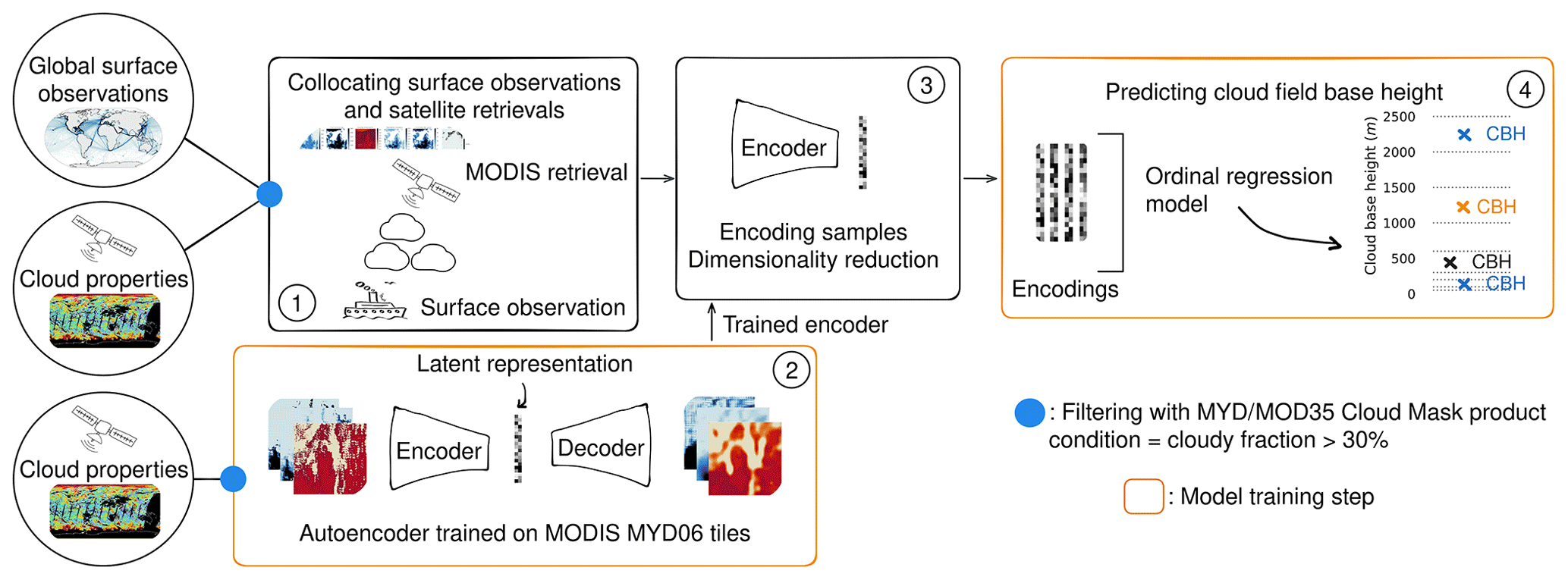
Figure 1 Schematic of the cloud base height retrieval method. (1) Collocation of surface-based cloud base height observations and satellite retrievals. (2) Auto-encoder training on satellite cloud properties. (3) Encoding of collocated samples using the trained encoder. (4) Prediction of the cloud field base height.

Section 2 firstly introduces the datasets and the collocation between ground-based observations and satellite retrievals. Secondly, the ML method constituting ORABase is described. In Sect. 3, we evaluate our predictions against other methods, including Noh et al. (2017) and other products from active satellite measurements like the 2B-CLDCLASS-lidar product (Sassen et al., 2008). Section 4 presents the global dataset of the CBH which is derived from the ML approach. We discuss the benefits and remaining challenges of our method in Sect. 5. Further details about the spatial distribution of the observations and the ML method are included in Appendices A–E. Additional links to available data outputs and codes are listed in the corresponding sections.

2 Data and methods

2.1 Surface observations

The CBH labels used in this study are part of a global marine meteorological observation dataset maintained by the UK Met Office (Met Office, 2006; Table 1), which provides ongoing observational data from 1854 onwards. The observations are conducted from measuring stations that were located on ships, buoys, or platforms. As a consequence, this study largely relies on observational data representing the areas along the corresponding ship routes (Fig. 2a). Despite their coarse resolution, the reported cloud base observations provide valuable information about clouds in remote marine areas. The distribution of CBH observations and corresponding bins are shown in Fig. 2.

Table 1 Dataset description. The surface observations are provided by a worldwide station network available from the UK Met Office (Met Office, 2006; see Sect. 2.1). The MODIS data are derived from collection 6.1 of the datasets (Platnick et al., 2017; Ackerman and Frey, 2017; see Sect. 2.2).

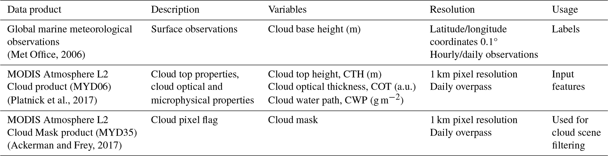
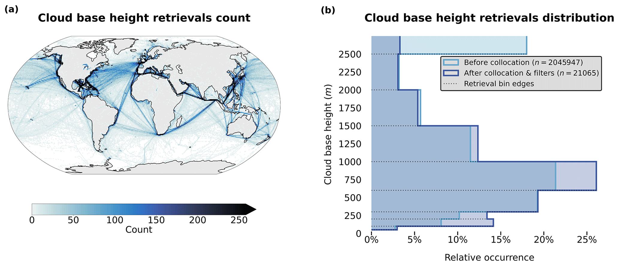
Figure 2 (a) Spatial distribution of cloud base retrieval counts (1° grid) and (b) distribution of the retrieved cloud base height before and after the collocation and filtering process for observations from the years 2008 and 2016.

At the beginning of meteorological and weather reports, surface-based cloud observations were retrieved manually or visually by human observers, but they have been gradually replaced by automated systems. In the surface observation dataset used in this study, the CBH is derived using a ceilometer, an instrument based on a laser pointing upright and measuring the backscatter from the cloud base, and is then reported following the current standards from the World Meteorological Organisation (WMO; WMO, 2019). The CBH observations are sorted into bins of increasing width (from 50 to 500 m bin width) corresponding to the altitude (Fig. 2b) as the data transfer through radio limits the amount of transferable information, and precision close to the surface is of importance, notably for aircraft. Since the actual measured CBH values are not available in the dataset, it is impossible to directly quantify a possible bias stemming from this binning process. In general, here, we can suspect that the available CBH retrievals represent an accurate or underestimated assessment of the effective CBH as, for example, a ceilometer measuring a CBH of 2490 m will report this to be in the 2000 m bin in the available dataset. Using, for example, the central value of each bin could be another way to compute averages to potentially alleviate this unknown bias, but this is not presented here. However, the method presented in the following sections predicts the CBH in corresponding bins; thus, it is left to the user to use these as they see fit for further analysis.

2.2 Satellite data

In this study, we use products from the Moderate Resolution Imaging Spectroradiometer (MODIS, Platnick et al., 2017) from the AQUA satellite as input data that are later combined with the CBH labels derived from the surface-based observations to train the prediction model. We choose MODIS satellite retrievals as they provide a large amount of data with kilometre-scale resolution and daily overpasses, with the spatial coverage of one granule representing an area of 2330 km × 2000 km. We make use of the CUMULO dataset (Zantedeschi et al., 2022) since it provides already preprocessed satellite data from the A-train with daily full coverage of the Earth for the years 2008 and 2016. In particular, out of the available variables, we use two aligned products (see Table 1), namely the MODIS Level-2 Cloud product (hereafter MYD06; Platnick et al., 2017), which provides relevant cloud properties, and the MODIS Level-2 Cloud Mask product (hereafter MYD35; Ackerman and Frey, 2017), which allows us to filter scenes and screen for clouds.

The MYD06 product contains various cloud top properties (temperature, pressure, height) and cloud optical and microphysical properties (optical thickness, effective radius, water path). Level-2 data are derived from calibrated radiances through various algorithms and physical relations detailed in Platnick et al. (2017). The cloud top quantities are derived from radiance data of several channels. Wavelengths in the CO₂ absorption range are particularly used to identify the cloud top pressure (CTP) and thus the CTH of high clouds because of the opacity of CO₂. For thicker or low boundary layer clouds, since the CO₂-slicing technique fails, the CTH is retrieved using the 11 µm brightness temperature band and is combined with simulated brightness temperatures based on vertical profiles from GDAS using surface temperature together with monthly averaged lapse rate data (Baum et al., 2012). The use of monthly averaged lapse rate data separately for different regions greatly helped reduce the bias in retrieved CTHs for low clouds in collection 6 compared to collection 5 of MYD06, but some spatial and regional biases remain. These biases directly impact the spatial and temporal distribution of CTH in the data and thus what the model could learn from. The cloud optical thickness (COT) and cloud effective radius (CER) are simultaneously derived from multispectral reflectances, cloud masks, CTP data, and surface type characteristics. The cloud water path (CWP) is additionally retrieved as part of the cloud optical property algorithm described in Platnick et al. (2017). The retrieval of these cloud properties additionally requires inputs such as temperature, water vapour, and ozone profiles from NCEP GDAS (Platnick et al., 2003; Baum et al., 2012), which can lead to potential uncertainties, in particular in remote marine regions, where only sparse observations are available for assimilation.

In general, the MYD06 level 2 product offers the advantage that the statistical model can be built relying on cloud properties, and it can thus allow the study of relationships between the CBH and other cloud properties. Calibrated radiances, one step ahead in the data-processing pipeline, would also provide insightful information but would require inputs of larger dimensionality since key information about clouds would be scarcer. Furthermore, using MYD06 level-2 data allows us to compare our method to others which, in most cases, use cloud properties to retrieve the CBH. From the entirety of available MYD06 retrievals, we select three cloud properties in particular, namely the CTH, COT, and CWP. The CTH is used as it provides key information about the CBH in the cloud field, as seen in Böhm et al. (2019). Vertically integrated cloud quantities like the COT and CWP further help the statistical model by providing key information about the cloud's vertical extent, lacking in the cloud top properties, making them commonly used for retrieving the CBH (e.g. Noh et al., 2017). The CWP as computed from COT and CER and, in consequence, the CBH are built on adiabatic assumptions (Grosvenor et al., 2018) and therefore cannot be used to constrain subadiabaticity, as also highlighted in Mülmenstädt et al. (2018).

2.3 Dataset collocation

We proceed to collocate our two data sources over the 2 years of available MODIS MYD06 data. To obtain the cloud properties of the cloud scene corresponding to the surface retrieval of CBH, we select a square tile of 128 km × 128 km from the closest MODIS granule available, centred around the observation location. Here, closest means that the MODIS granule contains the (latitude, longitude) coordinate of the CBH observation and the full extent of the tile it is centred around and that the satellite retrieval was made during a 1 h time window before or after the CBH observation time. The spatial and temporal thresholds used to collocate the surface observations and the satellite retrievals are chosen for several reasons. Mainly, we want the satellite cloud properties to be representative of the cloud scene for which the CBH observation was made. Additionally, we want to recover a satisfying number of samples during the collocation process. Further arguments regarding the sensitivity of the retrieval method to the tile size are described in the following (see Sect. 2.5).

The extracted tile corresponding to the surface observation is then filtered. A first filter is applied to missing values in the different cloud property fields to primarily avoid retrievals of poor quality. This is predominantly the case for the COT and CWP fields for which the retrieval fails more frequently, sometimes entirely. Another filtering is concordantly done using the MYD35 product for cloud cover (minimum of 30 % of cloudy pixels) to ensure that the cloud field is substantial enough for the collocated surface observation to be representative. Additional comments on the sensitivity of the CBH retrieval to this threshold are presented in the following section covering the downstream task of CBH prediction. Throughout the quality-filtering process, the missing data are one of the major factors impacting the number of retained samples. In Fig. 2, we can see that it seems to impact the clouds with higher CBHs.

The overall filtering and collocation processes yield around 21 000 samples. This only represents around 1 % of the initial CBH observations, mainly due to the collocation process both in time and space with the MODIS overpasses. Missing values and cloud cover filters are an additional factor in the reduced number of collocated samples. The presented collocated dataset is the basis upon which to build our cloud scene CBH retrieval.

2.4 Auto-encoder

To circumvent the lack of labelled samples from which the relevant features are extracted and to learn useful lower-dimensional representations of the data, we add a dimensionality reduction step to our method through an unsupervised learning model. AEs offer a wide application spectrum, ranging from preprocessing to the generation of new outputs. AEs are commonly used in unsupervised learning settings for reducing the dimension of the input data to leverage the latent representations learned by the model to perform clustering, classification, or regression in a lower-dimensional space (Baldi, 2012). We use classical AEs for their simplicity and versatility, but other approaches to unsupervised latent representation learning, such as variational AE and its many variants, can be used in a similar fashion. In general, AEs learn to encode the given input data to produce a latent representation of a lower dimension. From the latent representation, the input data are then reconstructed. The learning process is driven by what is called the reconstruction loss, which minimises the difference between the input and the reconstructed output.

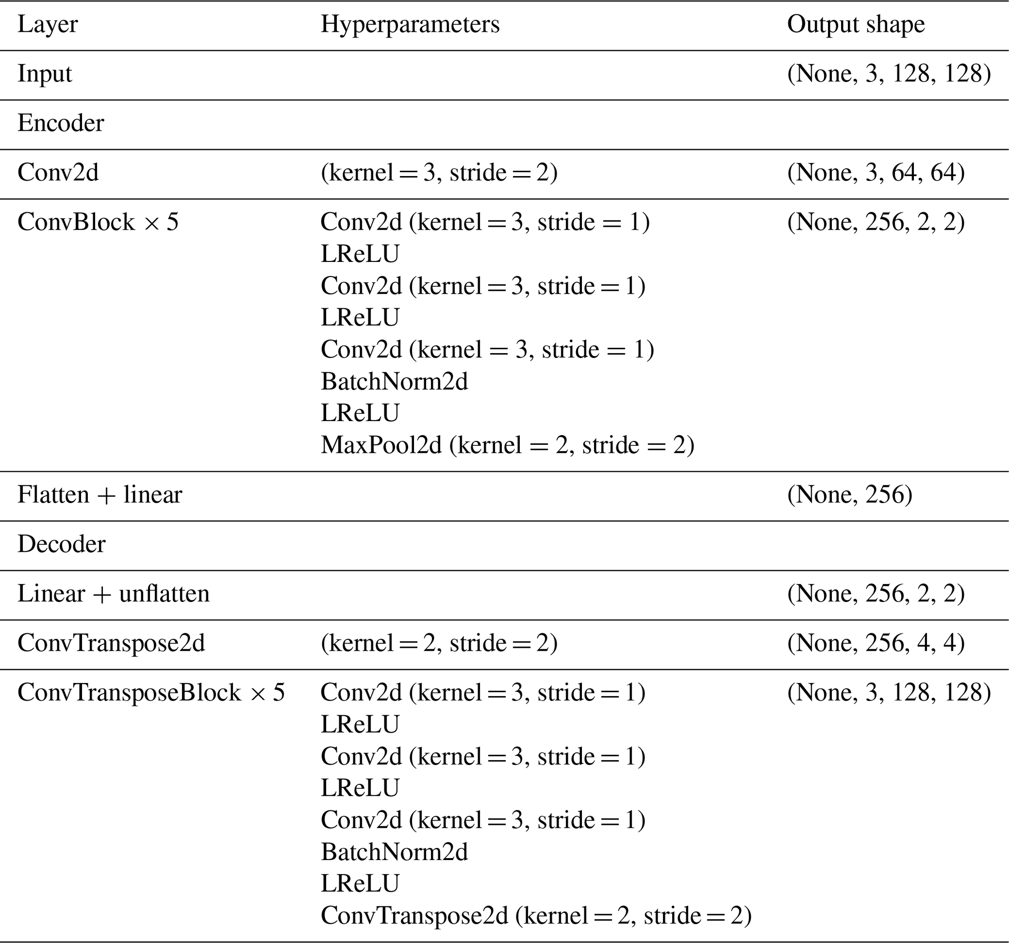
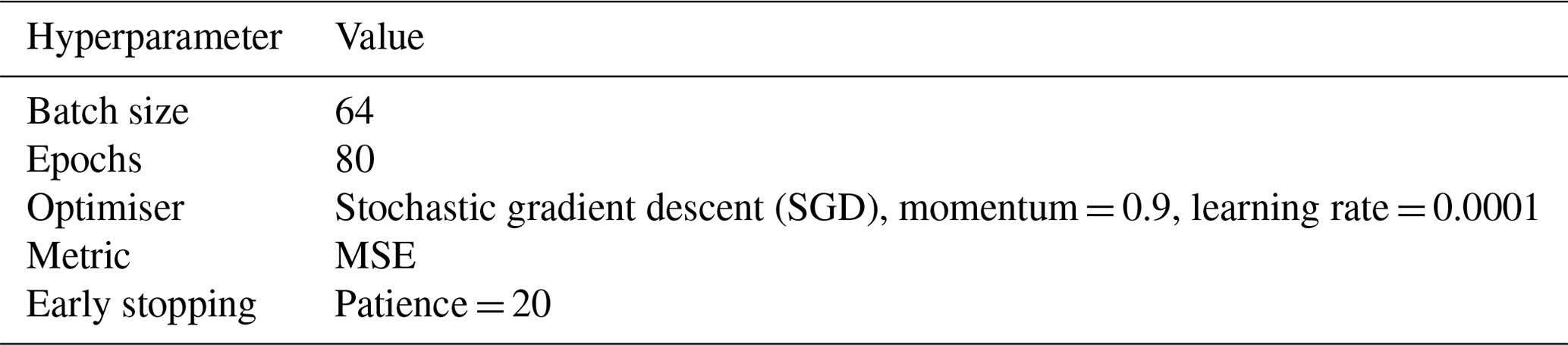
Here, we use a convolutional AE architecture which is based on a CNN backbone in order to leverage the spatial structure of our input data (Pu et al., 2016). We rely on the widely employed CNN architectures U-Net (Ronneberger et al., 2015) and VGG (Simonyan and Zisserman, 2015), where the convolution layers are based on 3 × 3 filters, stacked in blocks, followed by maximum-pooling layers and mirrored for the decoder part of the model using transposed convolution layers (Zeiler et al., 2010). We adapt the size of the input to fit our chosen tile size (128), and we adapt the latent space size to 256 and use the improved leaky rectified linear units (LReLUs; Maas et al., 2013) over the original ReLU (Nair and Hinton, 2010) as activation functions. The detailed parameterisation of the model is described in Appendix C. The model code was developed following implementations from the packages PyTorch (Paszke et al., 2019) and torchvision (torchvision maintainers and contributors, 2016) and is included in the related Zenodo archive (Lenhardt et al., 2024). The main goal of the AE training is then to minimise the loss function during the optimisation or learning process and to reproduce the input data with the highest fidelity. For the loss function which, in this case, is only the reconstruction error, we use the common mean-squared error (MSE), which can be written for a batch of samples as follows:

$$\begin{array}{}\text{(1)}& L_{\mathrm{reconstruction}}={\displaystyle \frac{\mathrm{1}}{N_i}}\sum _{b\in B_i}{\left|\left|b-D_{\mathit{\theta }}\left(E_{\mathit{\theta }}\left(b\right)\right)\right|\right|}_{\mathrm{2}}^{\mathrm{2}},\end{array}$$

where, with the tiles used for training the AE being noted as $B={\left\{b_n\in R^{\mathrm{3}\times \mathrm{128}\times \mathrm{128}}\right\}}_{n\in \left[\mathrm{1},N\right]}$, B_i represents a batch of samples of size N_i, and θ represents the combined parameters of the encoder E and decoder D models. The MSE considered here between the inputs and outputs of the AE is unitless as the inputs are standardised before processing to ensure that each of the channels are on similar scales and to ensure a more stable model training.

However, this self-supervised step requires a large amount of data that the AE can learn from. Therefore, we select 1 full year of data of MODIS granules from the CUMULO dataset (from the year 2008; see Sect. 2.2) and randomly sample tiles following the same criteria as during the collocation process (see Sect. 2.3). We sample a maximum of 20 tiles from a single granule, and this is done for only 1 single year of data in order to avoid possible spatial and temporal auto-correlations in the data used for training and testing leading to a non-representative performance of the mode (Kattenborn et al., 2022). Further details on the study of the generalisation performance of the model for new observations in space and time are given in Appendix B. Overall, the built dataset consists of around 500 000 samples which are then split for training, validation, and testing based on their retrieval date. For further testing, we additionally create a test dataset based solely on data from the year 2016, which include tiles not only over the ocean but also over land, indicating potential generalisation skill for unseen data including orography influence. The reconstruction error during training and validation is shown in Fig. 3, along with examples of reconstructed samples. The spatially averaged reconstruction errors per cloud property channel are displayed in Fig. 4 for each of the training, validation, and testing datasets previously mentioned. The trained model reaches an MSE of 0.19 on the test set of 2008 and of 0.24 on the global test set of 2016. The presented model is trained on tiles of size 128 × 128, but some arguments regarding the choice of the tile size are made in the following section in the context of the downstream task of CBH prediction.

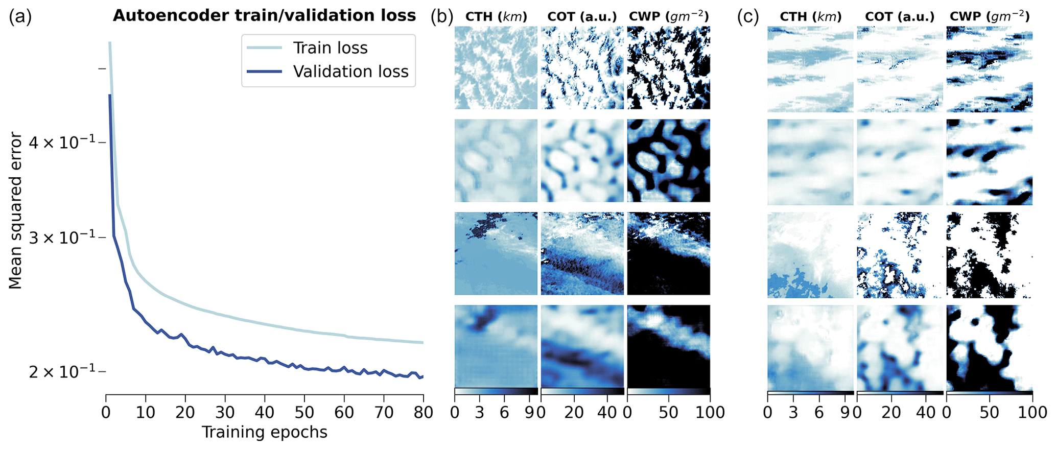
Figure 3 (a) Training and validation losses during model optimisation. (b, c) Examples of tiles (first and third rows) with the corresponding reconstructions (second and fourth rows) for the different cloud property channels.

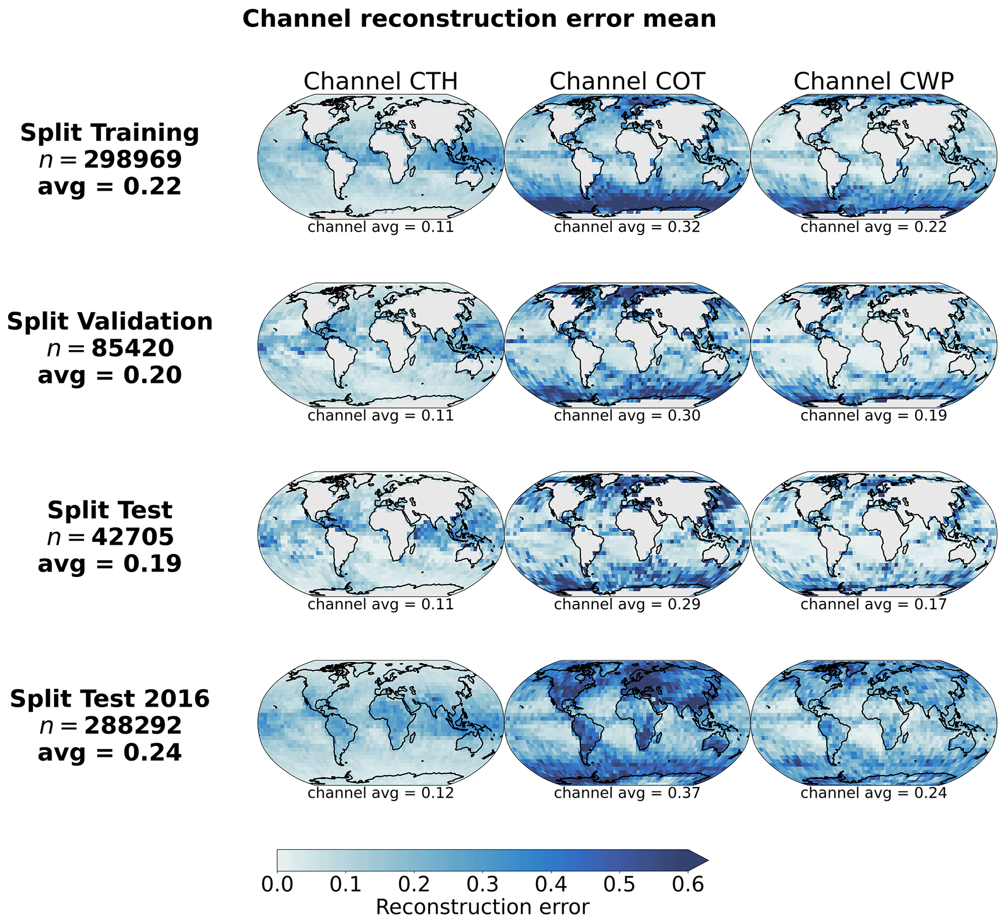
Figure 4 Spatial distribution of channel reconstruction errors aggregated on a 5° grid for the 2008 training, validation, and test datasets and for the 2016 test datasets.

2.5 Cloud base height ordinal regression

Once the AE's optimisation process is completed, the next step is to predict the corresponding CBH for the observed scene. As seen in Fig. 2, the retrieved CBH observations are binned into different categories following WMO standards (WMO, 2019). This leads to a prediction problem at the intersection of regression (i.e. predicting numerical values) and classification (i.e. predicting the object class) called ordinal regression (OR). The labels from the target variable are defined by classes following a certain order, in this case the increasing CBH. A wide array of methods stem from this field, with diverse applications in, for example, computer vision using neural networks (e.g. Niu et al., 2016; Shi et al., 2023; Lazaro and Figueiras-Vidal, 2023). Different methods exist to tackle such problem setups either via modification of the target variable, ordinal binary decomposition, or threshold modelling (Gutiérrez et al., 2016; Pedregosa et al., 2017). Threshold models were shown to be able to perform better than the ones designed for regression or multi-class classification on OR tasks (Rennie and Srebro, 2005). Here, we consider two alternative frameworks in the case of threshold models which differ in terms of how they penalise threshold violations: immediate-threshold (IT; Eq. D1) and all-threshold (AT; Eq. D2). The overall training process of the model aims to optimise a set of weights to project the input data to a one-dimensional plane, subsequently dividing the constructed representation using learnable thresholds. These two implementations of threshold models are available from the mord Python package (based on Pedregosa, 2015), and further details on threshold OR models are added in Appendix D.

To help evaluate the prediction model, we rely on a set of different metrics pertaining either to the regression aspect of the problem or to its classification and/or ordinal nature. First, the macro-averaged mean absolute error (MA-MAE) is used as it weights each class separately before averaging the subset MAEs, making it useful in the case of OR problems with imbalanced datasets (Baccianella et al., 2009). Using a macro-averaged metric prevents us from choosing a trivial model which might always predict the dominating class. Additionally, the macro-averaged root-mean-square error (MA-RMSE) is also used to investigate the skill of the prediction models. To assess the ordering of the predicted retrievals with respect to the labels, the ordinal classification index (OC; Cardoso and Sousa, 2011) and its updated version, the uniform ordinal classification index (UOC; Silva et al., 2018), are computed. A version of the latter not requiring an extra hyperparameter, the area under the UOC (AUOC; Silva et al., 2018), is also reported. These different metrics are able to capture the proper ranking order of the predictions compared to the labels using the confusion matrix and also the overall accuracy of the prediction model. Nevertheless, one caveat is that these indexes developed for ordinal classification assume each class to be equally distant from one another, which is not the case here since the CBH retrievals are reported in bins of variable width. However, a purely ordinal classification index will drop all information on the scale of the response (1500 m misclassified as 600 m treated the same as 200 m misclassified as 50 m since only the order matters), which might be not entirely appropriate for this problem. In an effort to address this limitation, the indexes are adapted to mimic the spacing between the different CBH bin classes by incorporating classes that are all spaced by 50 m, ranging from 50 m up to 2500 m. In this manner, the CBH class difference is more suited to the actual nature of the retrieval.

However, several aspects of the ordinal-regression model need to be investigated first. To this extent, we first divide our global collocated dataset (Sect. 2.3) into training, validation, and testing datasets but simultaneously ensure that each class is relatively equally represented in each split. The following aspects and sensitivities of the model to the input data parameters are assessed using the training and validation datasets: the potential benefit of using the spatial context through the AE, the input tile size, and the cloud cover threshold. Moreover, the spatial generalisation skill of the model is studied by splitting the collocated dataset between the Northern Hemisphere and the Southern Hemisphere. For each of these, the performance for the AT variant of the OR model is reported as it performs significantly better than the IT variant across experiments and evaluation metrics.

2.5.1 Spatial context

In order to evaluate the actual effect of the spatial context with respect to the input cloud properties, the prediction skill of the model trained based on the AE encodings is compared to a collection of three baseline methods: two trivial methods (predicting the majority bin and predicting the bin minimising the MAE across the training dataset) and an OR method relying on the flattened cloud properties of a 9 × 9 tile centred around the observation. Both of the trivial methods result in always predicting the CBH bin of 600 m. The third method yields a similar dimensionality as the AE encodings (three channels × 9 × 9 = 243) and thus helps to show how the AE potentially leverages some spatial information about the cloud scene. Across all metrics, the method using the 9 × 9 tile input is outperformed by the OR method based on the AE encodings and even by the trivial choice of the majority bin. It is, in particular, noticeable with an increase in the MA-RMSE by 400 m and in the MA-MAE by 140 m compared to the OR predictions made with the AE. On the other hand, considering the predictions made with the trivial method leads to an increase in the MA-MAE of 50 m but a decrease in MA-RMSE as most of the labels are actually concentrated around the 600 m bin. The mean bias of the trivial method is lowered closer to 0 m as it leads to a more substantial underestimation of the high CBHs and overestimation of the low CBHs. To conclude the comparison with these two other baselines, the information spatially encoded by the AE over the whole tile size area is useful in producing CBH retrievals of better quality compared to a baseline OR model with a reduced spatial context or a trivial method predicting a singular bin.

2.5.2 Tile size

A prediction model is fitted to the input data using encodings produced with tailored AE models trained as detailed in the previous section but with varying square input tile sizes of 16, 64, and 128. With the subsequent prediction models, the retrievals made with a tile size of 128 showcase the lowest MA-MAE (0.8 % and 2.7 % decreases compared to tile sizes of 16 and 64, respectively) and MA-RMSE (around a 5 % decrease compared to both other tile sizes), while no clear sensitivity arises from the OC, UOC, or AUOC. Examining the performance for each class separately indicates reduced errors (MAE and RMSE) for higher CBHs (above 1000 m) using the larger tile size of 128 and on par performance across tile sizes for lower CBHs. In the context of the presented CBH retrieval, the larger spatial information provided through the input tile seems to be useful for the subsequent CBH prediction task, leveraged with the help of the AE as shown previously.

2.5.3 Cloud cover

The collocated dataset is first filtered again with cloud cover thresholds of 10 %, 20 %, and 30 %. Each threshold respectively leads to datasets of 25 042, 23 034, and 21 065 samples, which are then further split into training, validation, and testing. For the validation set, while the decreases in MA-MAE (4.5 %) and MA-RMSE (10 %) with the 10 % compared to the 30 % cloud cover threshold indicate a potential benefit of lowering the threshold, investigating the MAE and class-wise MAEs creates a different picture: the benefit seems to marginally concern the higher CBH classes while hindering the performances of low CBHs, which, overall, explains the trend in RMSE notably. Considering the confusion matrices generated for each cloud cover threshold additionally shows that a lower cloud cover threshold results in a slightly increasing distribution shift of the predicted CBH classes towards higher CBHs, displaying a prediction cluster around 1000 m. Overall, the benefit of additional available samples when lowering the cloud cover threshold does not seem to directly lead to convincingly improved performance. Here, the main axis of improvement probably lies in the widening of the collocation process to ensure broader spatial and temporal coverage of the training dataset.

2.5.4 Spatial generalisation

Furthermore, in a similar way as for investigating the spatial generalisation ability of the AE, we split our collocated dataset between the Northern Hemisphere and the Southern Hemisphere. This way, we ensure a minimal number of samples in each spatial split (17 615 and 3450 for the Northern Hemisphere and the Southern Hemisphere, respectively) even though the spatial distribution patterns of the retrievals greatly differ. As a result, the lower number of samples in the Southern Hemisphere leads to some overfitting, with metrics systematically worsening when testing on the Northern Hemisphere. However, the Northern Hemisphere training displays fair generalisation skill with equal or improved metrics when testing on the Southern Hemisphere, for example an 8 % decrease in MA-RMSE; a 1 % decrease in OC; and stable MA-MAE, UOC, and AUOC. The class-wise performances for the two splits reveal the overall generalisation difficulty for higher CBHs (above 600 m) when training on the Southern Hemisphere as the labels relative to these classes are mostly present in the Northern Hemisphere (Fig. A3 in the Appendix). The ability of the model to generalise from the Northern Hemisphere labels reassures us of the overall skill of the model once trained on all the labels available.

In the following section, we present the results of the developed method alongside comparisons to previous retrieval approaches. In particular, we compare our retrieval to a method assuming an adiabatic cloud model (adapted from Goren et al., 2018; see Appendix E for implementation) and to the method from Noh et al. (2017). The former relies on the CTH retrieved from CALIPSO's Cloud-Aerosol LIdar with Orthogonal Polarization (CALIOP; Hunt et al., 2009) and CloudSat (Stephens et al., 2008) but also relies on the CWP and CTT retrievals from MODIS MYD06. However, in our own comparison study, we used all necessary variables, including the CTH, from MODIS MYD06. The latter method relies on piecewise linear relationships between MODIS CWP and the geometric thickness of the uppermost layer from CALIPSO and CloudSat stratified by MODIS CTH. The application of the method presented in Noh et al. (2017) is, however, done with CTH retrievals from the Suomi National Polar-orbiting Partnership (SNPP) VIIRS. The comparison to our method presented here is done by using the MODIS-, CALIPSO-, and CloudSat-derived parameters from Noh et al. (2017) but also using the MODIS-derived CTH to produce the final CBH estimate. In both cases, since these methods can be applied pixel-wise when a MODIS retrieval is available, we computed the retrieved CBH values and averaged them over the cloud scene.

3 Results, evaluation, and comparison to previous retrieval approaches

3.1 Cloud base height retrieval, evaluation, and comparison to previous retrievals

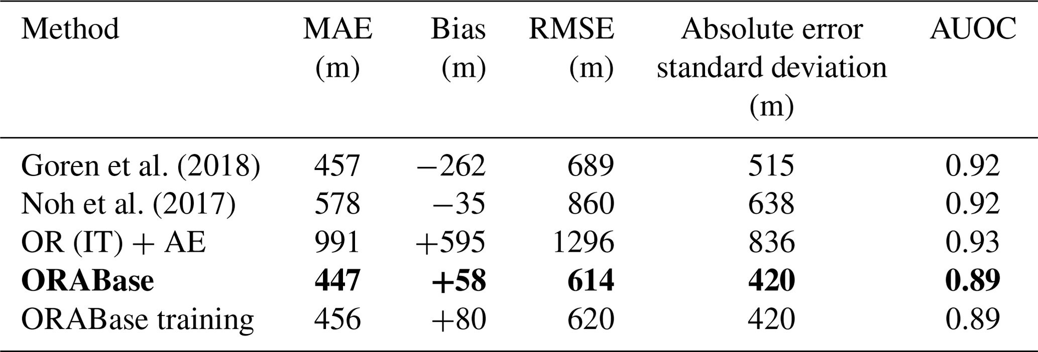
In this section, we present the results of the retrieval, evaluate it using the ground-based observations, and investigate how our method fares by comparing it to a method assuming an adiabatic cloud model (adapted from Goren et al., 2018; see Appendix E for implementation) and to the method from Noh et al. (2017). The analysis is performed for the collocated scenes where ground-based observations are available. To be able to compare the relevant metrics for the different methods, we proceed to a binning of the data following the WMO standard presented in Sect. 2.1. In Table 2, we report several metrics including the MAE, the mean error (bias), the RMSE, and the standard deviation of the absolute error. The latter helps us characterise the spread and uncertainty in the overall predictions with respect to the surface observations. We additionally report the adapted version of the AUOC mentioned in Sect. 2.5. Furthermore, we do not report quantities such as the correlation coefficient or the regression line on the two-dimensional histograms of Figs. 5 and 6 as the stratified and categorical aspects of the data would make reporting these not clearly informative. We refer to the overall conceived method including the AE (see Sect. 2.4) and the OR prediction model in the AT variant (see Sect. 2.5), listed in Table 2 as ORABase.

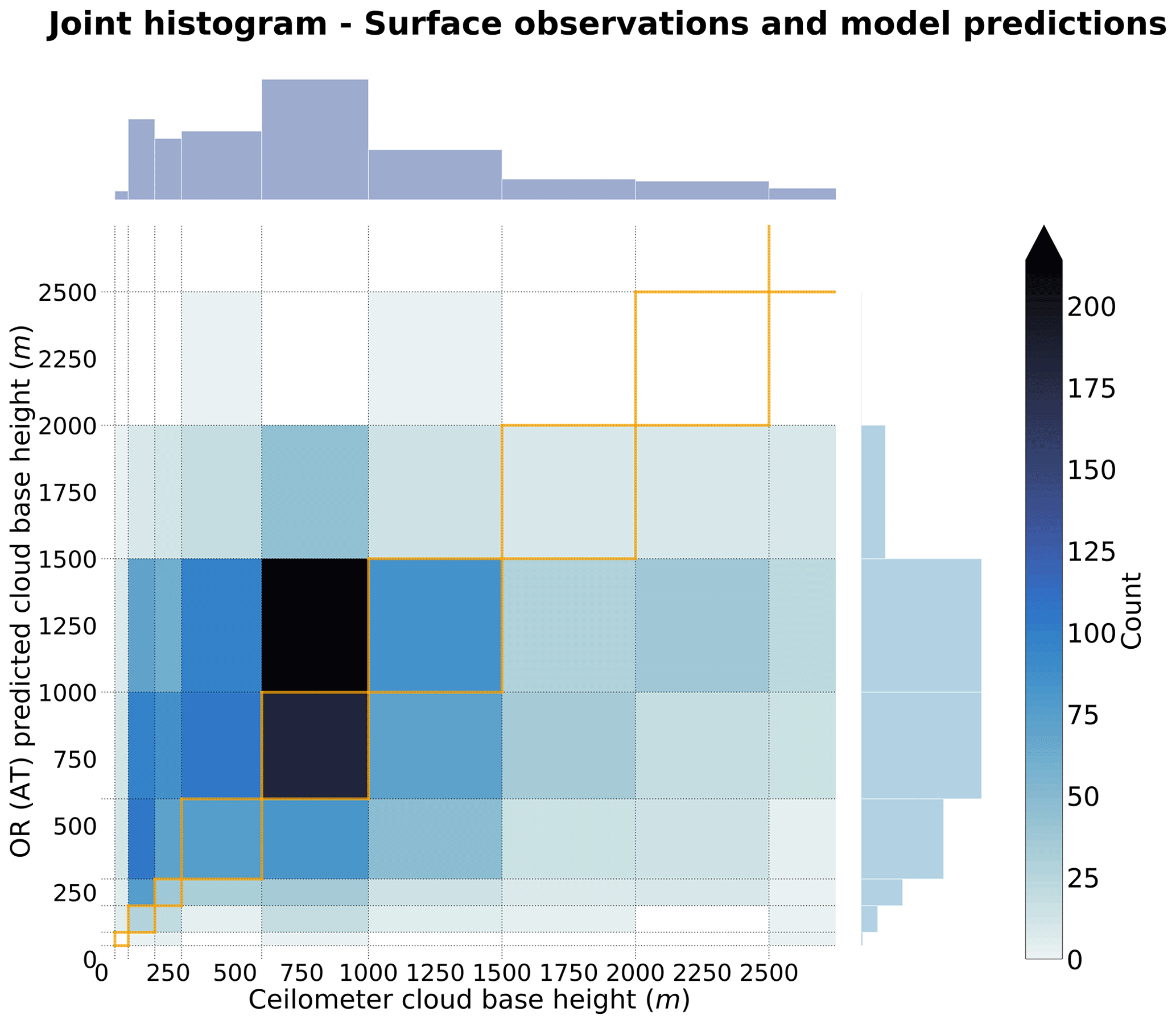
Figure 5 Joint histogram over the test set of the surface observations and the predicted cloud scene base height from ORABase with the ordinal-regression all-threshold model. The 1:1 boxes are highlighted in orange in the figure.

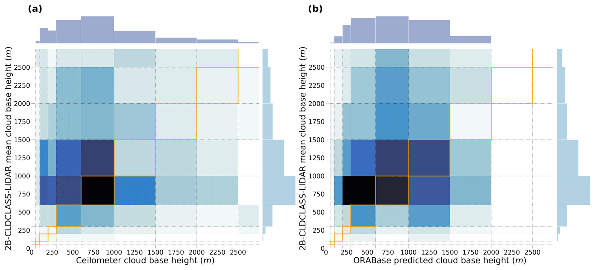
Figure 6 Joint histogram of (a) surface observations and 2B-CLDCLASS-lidar retrievals and (b) ORABase predictions and 2B-CLDCLASS-lidar retrievals for the collocated cloud scenes during the year 2008. The 1:1 boxes are highlighted in the figure in orange.

We first note that the OR method with an immediate-threshold setup fails at adequately predicting the cloud scene base height compared to all the other retrieval products, producing large errors (double-fold in comparison to the all-threshold setup). On the other hand, ORABase performs well with satisfying error measures and uncertainty in the predictions, on par with if not better than the two retrievals from Goren et al. (2018) and Noh et al. (2017). Compared to the method from Noh et al. (2017), our method succeeds in decreasing the error on average, displaying a reduction of 100 m for the MAE. The method also effectively diminishes the uncertainty in the CBH retrievals, bringing the absolute error standard deviation 200 m lower. Our method thus provides accurate retrievals with comparatively low general uncertainty levels. Even though, on average, the predictions exhibit a slight positive bias, we find that the CBH values above 2000 m are systematically underestimated (Fig. 5). In consideration of the low representation of such observations in the dataset, due to data filtering and surface observations being less reliable for higher clouds, the method still struggles to properly quantify the cloud scene base height of these samples. These samples also make up for most of the measurement uncertainty in the labels considering the fact that ceilometers face challenges for retrieving cloud signals higher up in the boundary layer. Focusing on lower cloud scene base height retrievals, the predictions demonstrate even lower errors: the MAE is lowered to 379 m, while the absolute error standard deviation is narrowed down to 328 m. Achieved accuracy levels and uncertainty measures attest to a certain trustworthiness of the cloud scene base height estimates, particularly in the context of product requirements – for example, the ones outlined by the Joint Polar Satellite System (JPSS; Goldberg et al., 2013; 2 km accuracy threshold). However, the cloud scene base height retrieval method presented here does not aim to constitute a product on its own as it is not operational in terms of the processing of new daily data available from the MODIS instrument; rather, it is operational in terms of the provision of robust estimates of CBH for lower-level clouds. Therefore, it is expected and reasonable that the accuracies and uncertainties presented here are below such thresholds. However, the available method code (Lenhardt et al., 2024) easily allows the processing of new data for users in addition to the available dataset for the year 2016.

We performed further sensitivity studies on our retrieval method, trying to improve the quality of the predictions. However, an attempt to balance the dataset by oversampling the higher CBH values (cloud base retrievals falling into the 2500 m bin) did not yield better results overall but also posed a higher risk of overfitting to these specific samples. Furthermore, any spatial information about the location of the satellite retrieval was not included so as to prevent possible overfitting to the latitude and longitude coordinates of the observations present in the training data. Since the observations are sparsely distributed, especially in the Southern Hemisphere (see the figures in Appendix A), the goal is to avoid any kind of induced spatial bias and sensitivity in the model's predictions. Accordingly, we can then ensure proper generalisation skill to new spatial areas but not only based on known retrieval distributions at similar locations. As a consequence, the choice was made to evaluate the potential generalisation skill of the prediction model by establishing a geographic distribution of the mean predicted cloud scene base height for a whole year's worth of MODIS overpasses. This is discussed in more detail in Sect. 4. On the other hand, the temporal aspect of the model's generalisation skill was intrinsically ensured by building a test set that was temporally distinct from the training set, including collocated samples from only the last months of 2016.

Table 2 Performance based on the test set of different CBH retrieval methods. OR models are either built with the immediate-threshold (IT) or all-threshold (AT) variant. The method on which the rest of the study is based has been highlighted in bold, and its corresponding performance based on the training set is added in the last row.

3.2 Comparison to spaceborne radar–lidar retrievals of the CBH

The combined datasets which are part of CUMULO (Zantedeschi et al., 2022), particularly the radar and lidar retrievals, facilitate the joint evaluation of our method with both ceilometer surface observations and active satellite retrievals. Specifically, we leverage the 2B-CLDCLASS-lidar product (Sassen et al., 2008), which is derived from the combination of CloudSat's Cloud Profiling Radar (CPR; Stephens et al., 2008) and CALIPSO's Cloud-Aerosol LIdar with Orthogonal Polarisation (CALIOP; Hunt et al., 2009). The base height of the lowest cloud layer retrieved by the instruments in each scene is considered to be the scene CBH and is then averaged over the available pixels along the track, preserving the same spatial extent as the associated cloud properties from the MODIS instrument. For the collocated samples of the year 2008, we thus jointly retrieve the obtained CBH from the 2B-CLDCLASS-lidar product, only considering cases where a surface observation was in the vicinity of the satellite track (inside a disc with a ∼ 60 km radius around the surface observation; see Sect. 2.3). For the samples fulfilling these conditions, we then compare how the different retrievals fare. In Fig. 6, the joint histograms for the surface observations, the 2B-CLDCLASS-lidar retrieval, and the method's corresponding predictions are documented, representing a total of around 800 samples.

Investigating the joint histogram between the surface observations and the 2B-CLDCLASS-lidar retrievals (Fig. 6a) allows us to identify shortcomings of the active satellite retrievals, particularly close to the surface (Tanelli et al., 2008; Marchand et al., 2008). Indeed, the CBHs closer to the surface are not well captured by the 2B-CLDCLASS-lidar retrievals, as partially expected, due to thick clouds attenuating the lidar signal and due to ground clutter and a lack of sensitivity to small droplets near the cloud base for the radar signal. A similar explanation can eventually be articulated as a whole for the collocated retrievals, considering the fact that the mean bias between the two retrievals is greater than +600 m. Concurrently, it is fruitful to compare the 2B-CLDCLASS-lidar retrievals with the predictions from the developed method (Fig. 6b). As seen previously, ORABase struggles at higher CBHs, but, here, it agrees reasonably well with the active satellite retrievals, especially for retrievals between 500 m and 1500 m. Focusing on retrievals under 1.5 km, the prediction model achieves similar performance compared to that presented in Table 2, with an MAE of 488 m and an RMSE of 576 m, even though the subset here is much smaller.

Furthermore, we created a more extensive dataset using only 2B-CLDCLASS-lidar retrievals and the cloud scene predictions with the aim of obtaining a more complete view of the relationship between these two retrievals. To this extent, we collated around 160 000 samples of aligned cloud scene base height predictions and the 2B-CLDCLASS-lidar retrievals over the year 2016. For this dataset, the performance metrics exhibit similar values as for the previously presented subset, displaying even lower values for the MAE and the absolute error standard deviation (around a 50 m decrease for both). Similarly to the previous collocated subset, limiting the evaluation to lower cloud base retrievals yields performance metrics close to a 450 m MAE and a 270 m absolute error standard deviation, both of these being mainly impacted by agreeing retrievals in the 500 to 1500 m range.

4 Global distribution

To further evaluate the method, we also apply the prediction model on global MODIS data for the whole year of 2016. The sampling process yields approximately 700 000 CBH retrievals for the corresponding cloud property tiles. We then spatially aggregate the predictions to a regular grid of 5° and compute the annual mean per grid cell along the annual median absolute deviation (MAD). The MAD constitutes a useful metric to quantify the variability while removing the effects of outliers. For more robust evaluations and statistics, only ocean grid cells with more than 100 CBH retrievals over the year are displayed, thus impacting mostly coastal and polar regions where filtering for ocean-only scenes or the original number of satellite retrievals leads to a higher rate of displaying removal. The spatial distribution of the mean cloud base (Fig. 7a) is similar to the outlined global distributions from other studies using different instruments and methods (Böhm et al., 2019; Lu et al., 2021; Mülmenstädt et al., 2018). The illustrated global quantities were established using MODIS overpasses which happen at a practically constant local time (13:30, early afternoon for AQUA). The MAD pattern exhibits similar characteristics (Fig. 7b), even though variability increases slightly in the vicinity of land masses. These interpretations still remain valid when looking at relative deviations. Typical features are lower cloud bases towards polar regions and the mid-latitudes and higher ones in the tropical regions. One can further observe regions like the Pacific coast of South America or the Namibian coast, which display lower cloud bases concurrently with lower variability (also highlighted in Lu et al., 2021). It is, however, impossible to follow up the study for nighttime retrievals as some MODIS cloud properties are not retrieved then.

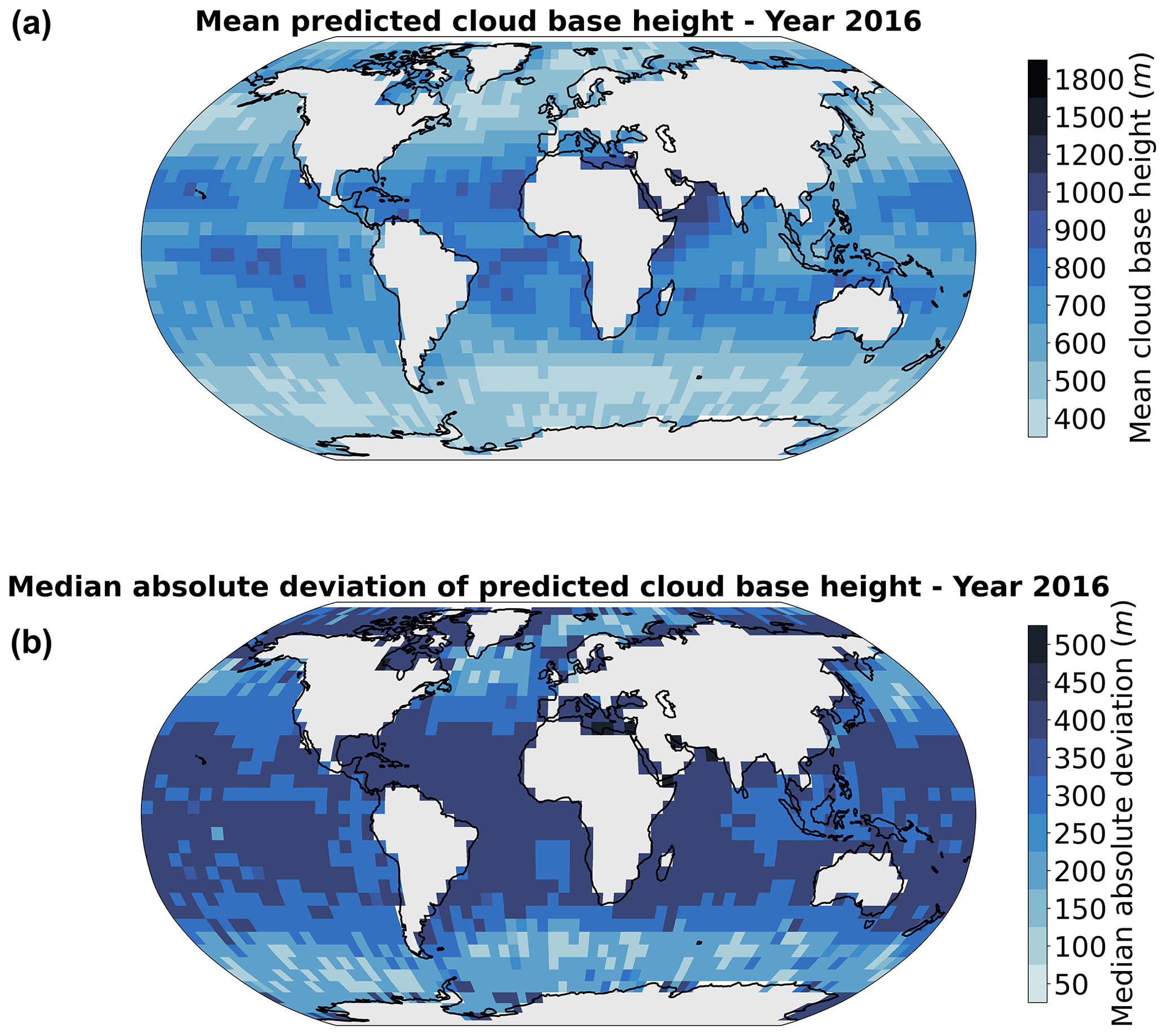
Figure 7 Spatial distribution of (a) mean and (b) median absolute deviations of predicted cloud base height for the MODIS data of the year 2016 aggregated on a 5° grid.

5 Conclusion

Here, we have presented a novel method named ORABase, which retrieves the cloud scene base height over marine areas from MODIS cloud properties, specifically CTH, COT, and CWP. This method can produce robust CBH estimates for cloud scenes, particularly for lower cloud bases (MAE of 379 m and absolute error standard deviation of 328 m for up to 2 km cloud bases) based on the assumption of a homogeneous cloud base across the considered cloud field. The statistical model was built on surface observations of cloud bases with ceilometers (Sect. 2.1) and then evaluated in comparison to other methods using passive satellite instruments (Sect. 3.1) and active satellite retrievals (Sect. 3.2). Analysis of the yearly averaged CBH (Sect. 4) helped to make further sense of the predicted cloud bases and variability. The global dataset for the year 2016 is available from Zenodo (Lenhardt et al., 2024).

Using the spatially resolved information of cloud fields of CTH, COT, and CWP through the described CNN-AE results in more accurate CBH retrievals compared to the active retrievals of the 2B-CLDCLASS-lidar product, producing better performance metrics compared to the other products and methods considered in this study. The combination of a CNN-based AE to reduce the dimensionality of the spatial patterns of cloud properties with a simple OR model leads to a better CBH retrieval compared to previous presented methods. The OR modelling helps in bridging the gap between regression and classification, facilitating the use of the binned cloud base observations provided by the surface observation dataset. Overall, ORABase achieves low error in the retrievals, around 400 m, and concurrently achieves a narrow absolute error distribution, more precisely around 400 m absolute error standard deviation. Both of these performance metrics are additionally reduced when focusing on cloud bases lower than 2 km. Application to data over land areas has not been processed yet but would certainly require adding surface observations from land during the training process (e.g. Böhm et al., 2019; Lu et al., 2021; Mülmenstädt et al., 2018). Application of the presented retrieval method to other instruments could also be considered. Incorporating TERRA MODIS data would help constrain the annual mean estimates presented in Fig. 7 by partially removing the potential bias of the single daily overpass arising from using only AQUA data presented in this study. The aspect enabling potential application of the retrieval method to different instruments outside of the two MODIS sensors would be the standardisation process for the input cloud properties before the use of the AE, which is done based on means and standard deviations computed from AQUA-only granules. Carefully investigating the characteristics of the distribution of the cloud properties from another instrument to ensure proper scaling when using the trained AE would then be necessary. Further tests could be done in addition using a coarser resolution for the input cloud properties.

Furthermore, classical semi-supervised pipelines like the one presented here, characterised by a small labelled dataset and a vast unlabelled dataset, necessitate a kind of collocation or matching process which often proves to be cumbersome and generates only a limited number of labels. However, future avenues of research could consider directly modelling unmatched datasets, as in, for example, Lun Chau et al. (2021) with multi-resolution atmospheric data, by making use of other quantities present in the observations as mediating variables to model the link between observed and unobserved variables.

In essence, the main benefit of producing better cloud base estimates is to gain accuracy in the overall retrieval of cloud geometry, impacting, in particular, radiation estimates (Kato et al., 2011) like the surface downwelling longwave radiation (Mülmenstädt et al., 2018). ORABase can thus prove to be useful by helping to produce CBH with enhanced confidence at a global scale.

Appendix A: Cloud base height retrieval distribution

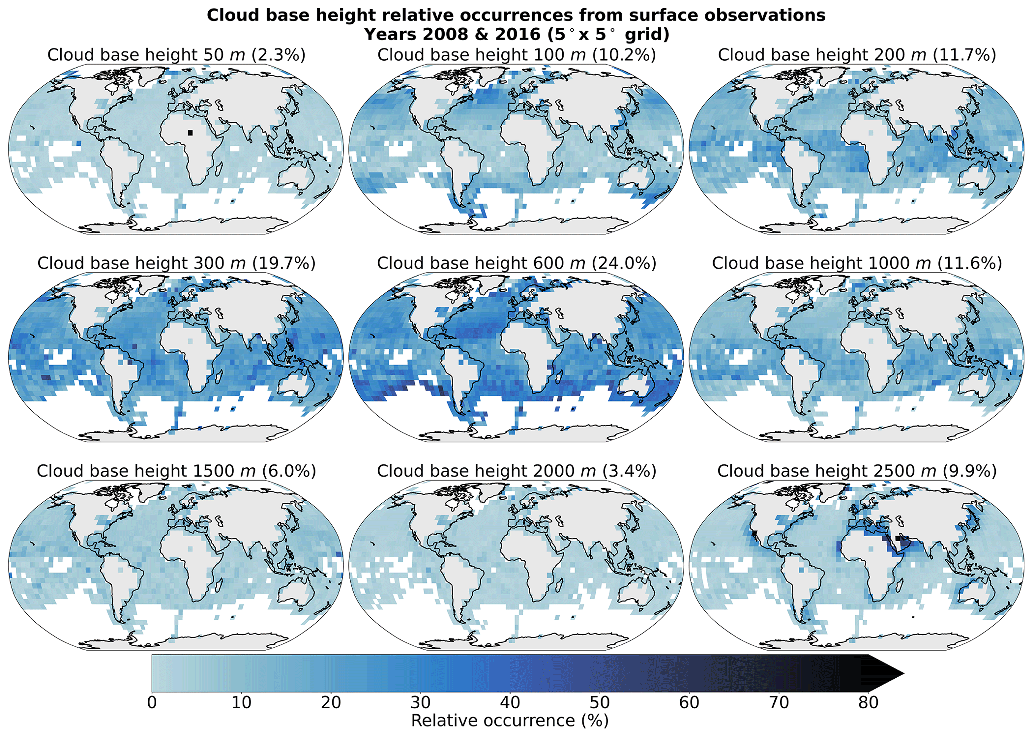
Figure A1 Spatial distribution of cloud base height retrievals (Met Office, 2006) for the years 2008 and 2016 on a 5° grid. The overall percentage of each label in the total observations is indicated in brackets. Only grid cells with more than 50 retrievals are displayed.

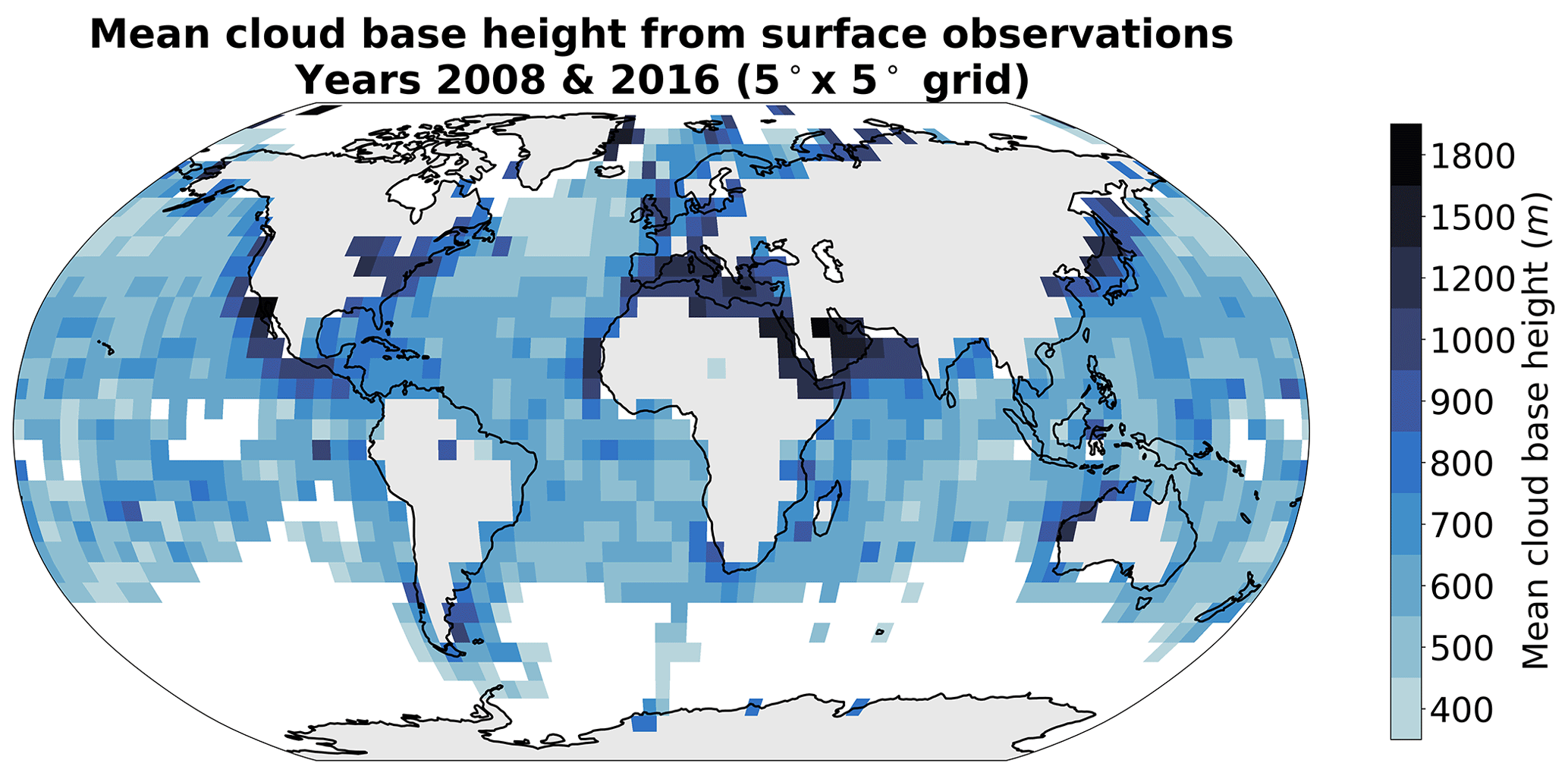
Figure A2 Mean cloud base height from retrievals (Met Office, 2006) for the years 2008 and 2016 on a 5° grid. Only grid cells with more than 50 retrievals are displayed.

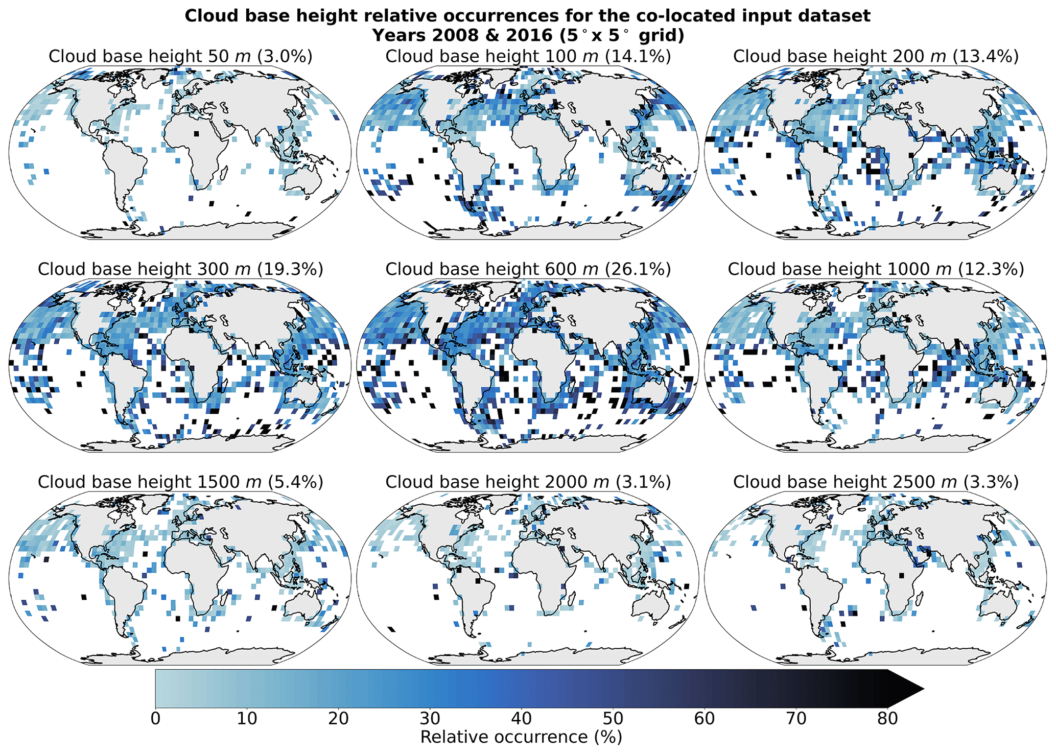
Figure A3 Spatial distribution of the collocated cloud base height retrievals (Met Office, 2006) and the satellite cloud properties used for training the prediction model for the years 2008 and 2016 on a 5° grid. The overall percentage of each label in the total dataset is indicated in brackets.

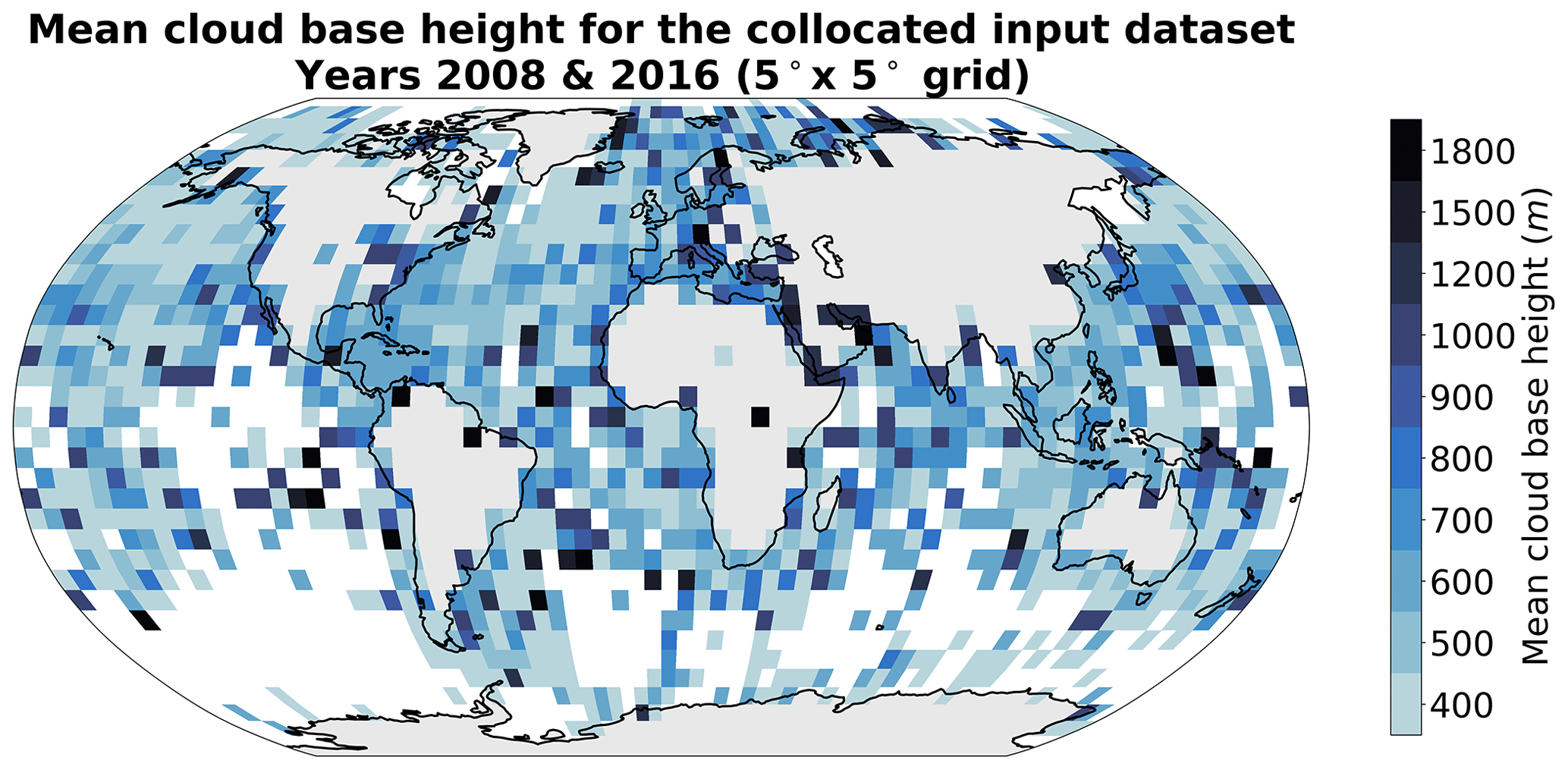
Figure A4 Mean cloud base height from the collocated retrievals (Met Office, 2006) and the satellite cloud properties used for training the prediction model for the years 2008 and 2016 on a 5° grid.

Appendix B: Spatio-temporal correlation study

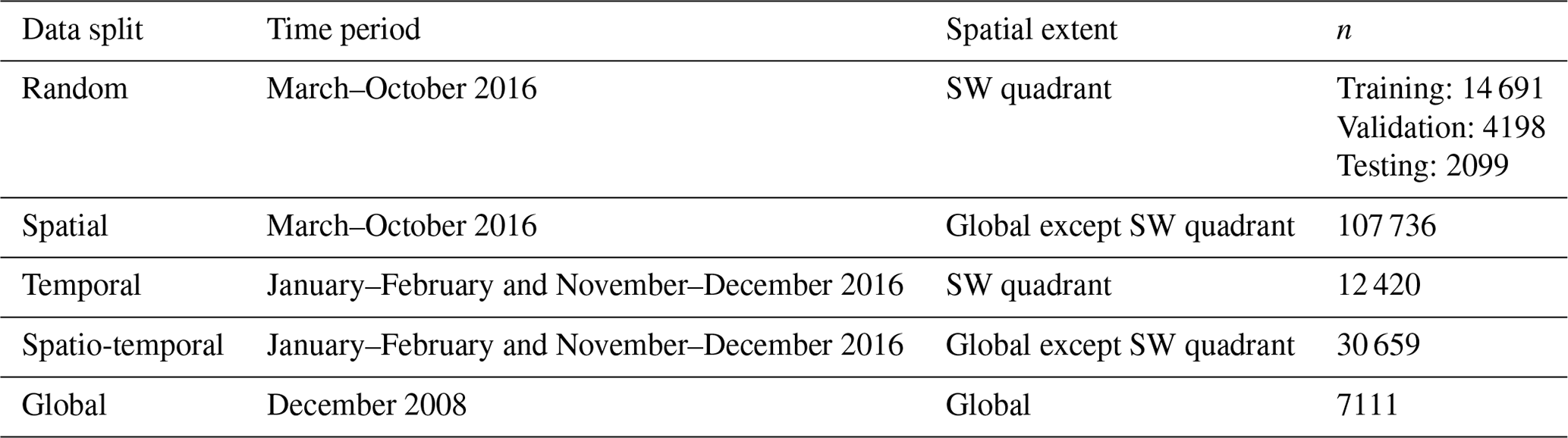
We create five different datasets to evaluate how capable the chosen AE architecture is of generalising to new data while trying to remove some possible autocorrelation biases which might inflate the performance scores. We also use this study to analyse how the AE model behaves when trained with our input data. We define two splits for space and time in order to build the training and testing datasets, namely the southwestern (SW) quadrant and the period from March to October, respectively. The granules used to build the datasets span across the whole year of 2016. The random data split is the basis for the training of the model and consists of tiles sampled in the aforementioned quadrant and time period. These tiles are then split randomly between training, validation, and testing datasets. This split represents the common way of splitting data when building an ML model. In contrast, we build three other datasets which vary through their respective spatial and time spans. The spatial split is built considering tiles spanning across a distinct time period, here between November and February, regardless of their spatial location. The temporal split is built considering tiles located anywhere but in the southwestern quadrant regardless of the time at which the retrieval occurred. Finally the spatio-temporal split combines the previous two conditions in order to build a dataset in which the tiles come from an independent location and time compared to the ones used for training. Additionally, we create a global data split using data from a different year, here 2008, without any spatial restriction for the tiles. Furthermore, only a limited number of tiles were extracted from each granule, while only granules from non-consecutive days were used in order to limit possible correlation between the extracted scenes.

Table B1 Name, time period, spatial extent, and number of samples for each of the five described data splits.

We then train an AE model using the training data from the first data split (random). Each test data split is then used to evaluate the trained model through the reconstruction errors divided by the reconstruction error mean of the random split (noted as the reconstruction error ratio; Fig. B1). The spatial distribution of the mean reconstruction errors is shown in Fig. B2. We detail in Table B2 the average channel reconstruction error for each of the splits.

Table B2 Average channel reconstruction error for each of the five described data splits.

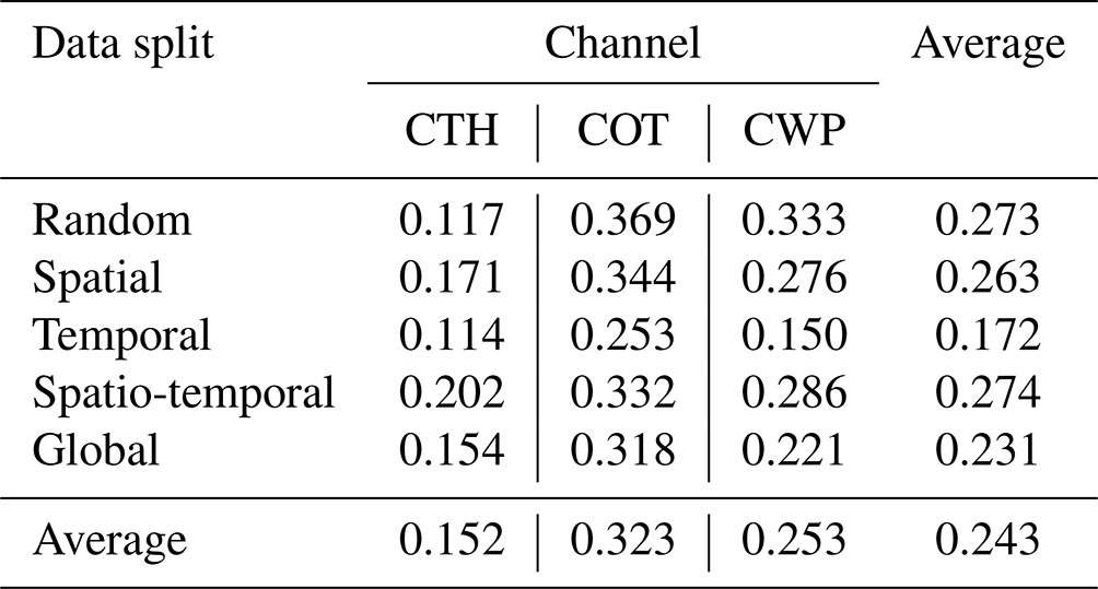
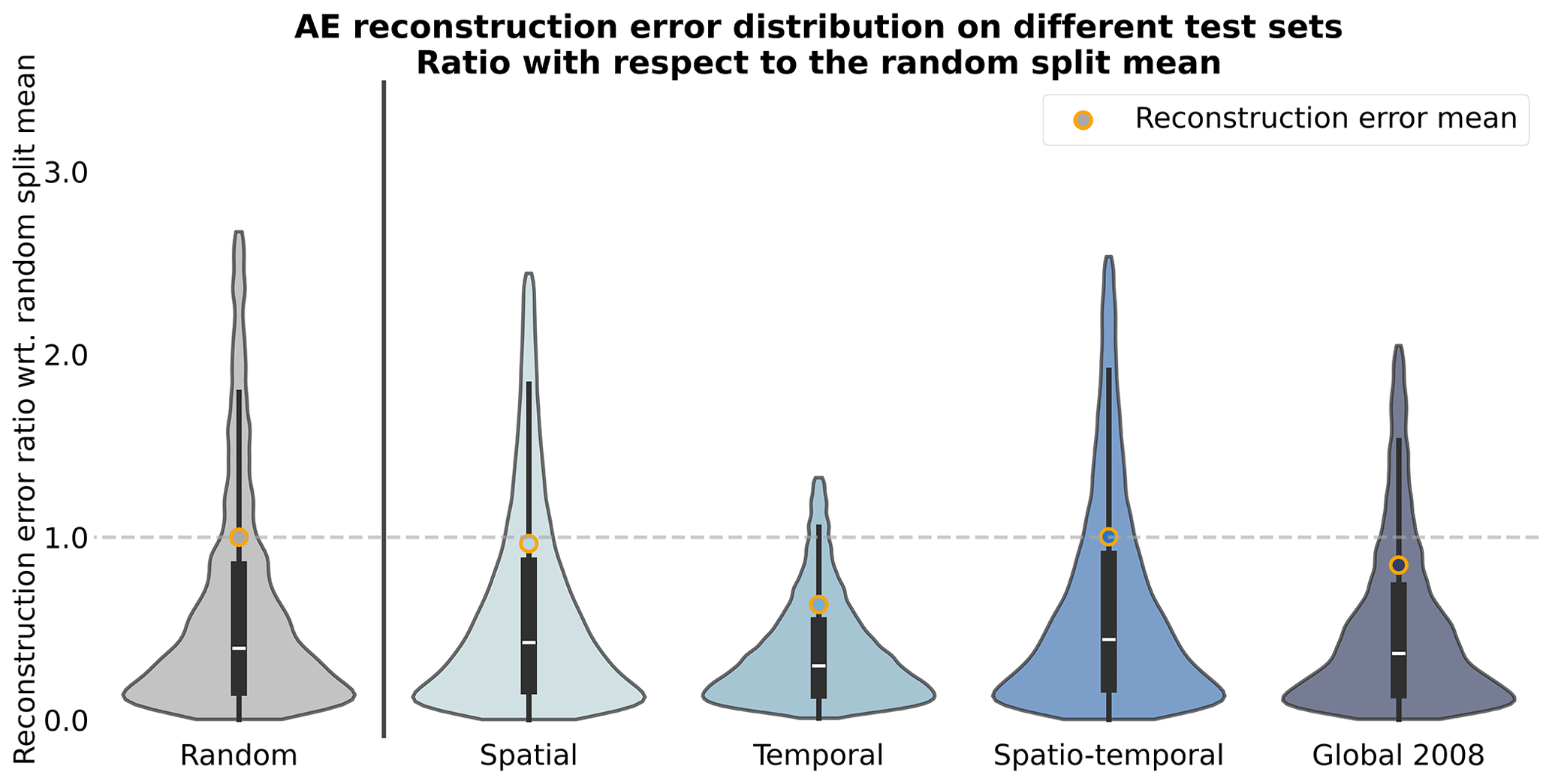
Figure B1 Reconstruction error ratios of an AE for different test datasets. The quartiles are indicated with the bar plot inside each violin plot, while the mean is indicated with an orange circle. Extreme values were removed before plotting. Each sample's reconstruction error is divided by the mean reconstruction error of the random data split and defines the reconstruction error ratio presented here.

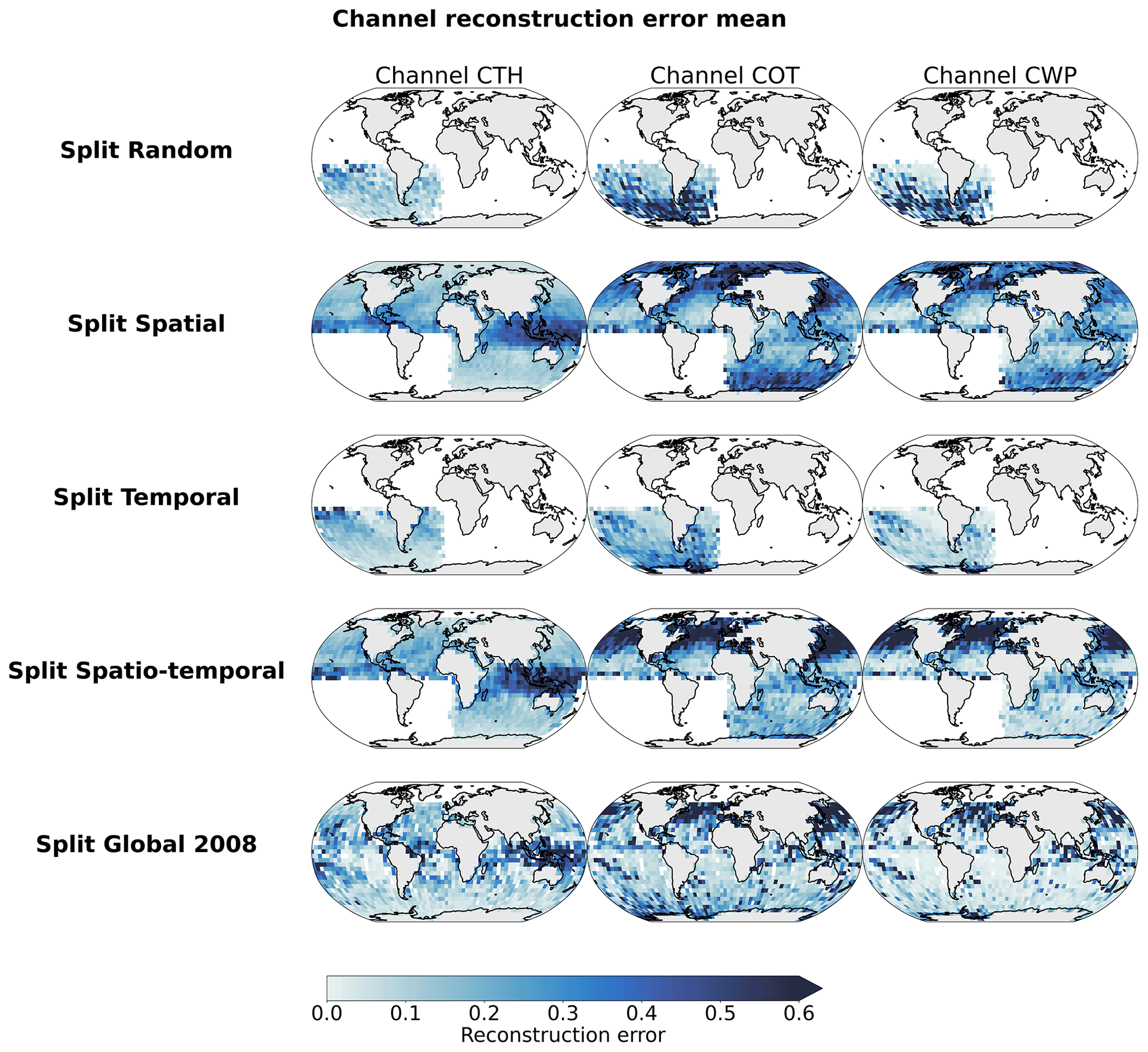
Figure B2 Distribution of mean channel reconstruction errors aggregated on a 5° grid.

We first notice that the reconstruction power of the model is consistent regardless of the test split considered, with mean reconstruction error ratios ranging from 0.63 to 1.0, dividing the split's reconstruction error by the random data split's mean reconstruction error. Ratios around 1 or below indicate that the model's performance is not inflated when considering a random data split, highlighting that the model did not learn from only possible spatial and/or temporal correlations between samples present in the training set. The distribution of the error is also very similar throughout the test splits, with most of the samples located below an error ratio of 0.5. However, one of the main aspects with regard to the performance of the model across test splits is the presence of a heavy tail in the distribution, showcasing that, for some samples, the reconstruction error can be greater than 3 times the mean error. Looking at the spatial patterns of the reconstruction error, we note that, overall, the error comes from the COT and CWP predictions, with the average reconstruction errors across test sets being 0.15, 0.32, and 0.25 for CTH, COT, and CWP, respectively (Table B2). For the CTH, the error is concentrated in the zones with frequent convection around the Equator and could be explained by local convection cells exhibiting a larger spread in CTH values. Another source of error could be that higher CTH values are also less represented in the training data. On the contrary, the error for COT and CWP prevails in high-latitude regions. Overall, the performance skill of the AE model seems to hold through the different test data splits. One could argue that the training dataset already retains enough variability in the data, which could explain why the model still performs well regardless of the test set split. However, this consistent skill also shows that the performance reported in Appendix C based on the test set can be trusted to hold for other datasets and supports the data generation process to train the AE (see Sect. 2.4).

Appendix C: Auto-encoder architecture

Table C1 Auto-encoder model specifications.

Table C2 Auto-encoder model training specifications.

Appendix D: Ordinal regression

We define our labels y, which can take values of K (nine classes): $\left\{\mathrm{50}\mathrm{m},\mathrm{100}\mathrm{m},\mathrm{\dots },\mathrm{2500}\mathrm{m}\right\}$. We introduce K−1 thresholds α_y to define the separation of our K classes; here, the thresholds actually correspond to the classes too. For each labelled sample (s,y), the output of our model is z=z(s). The correct interval for this sample is then $\left({\mathit{\alpha }}_{y-\mathrm{1}},{\mathit{\alpha }}_y\right)$. During the fitting process, the goal is to find the set of parameters of our model z and the corresponding thresholds α, which minimises a certain cost function. We consider a generic non-negative penalisation function f(⋅) (e.g. hinge loss, squared-error loss, Huber loss). There are then different ways to represent threshold violations and thus to penalise the predictor. While the immediate-threshold setup only considers the thresholds of the correct interval, the all-threshold setup takes into account all the threshold violations. In the case of an immediate-threshold setup, the loss function would look like the following:

$$\begin{array}{}\text{(D1)}& L(z,y)=f\left(z-{\mathit{\alpha }}_{y-\mathrm{1}}\right)+f\left({\mathit{\alpha }}_y-z\right).\end{array}$$

Here, we can see that the loss is not aware of how many thresholds are actually violated. In the case of an all-threshold setup, the loss function is a sum of violations across all thresholds:

$$\begin{array}{}\text{(D2)}& L(z,y)=\sum _{i=\mathrm{1}}^{K-\mathrm{1}}f\left(t(i,y)\left({\mathit{\alpha }}_i-z\right)\right),\end{array}$$

where $t(i,y)=-\mathrm{1}$ if i<y or +1 if i≥y. Thus, predictions are encouraged to violate the lowest number of thresholds.

We give in Fig. D1 an example of what the loss function would look like in the case of K = 6 and using a hinge penalisation.

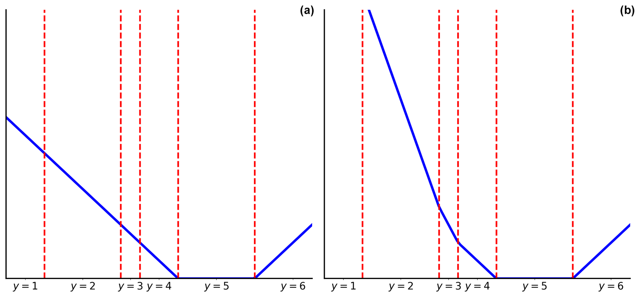
Figure D1 Threshold-based setup loss function representation for a hinge penalisation, K = 6, and target label y = 5. (a) Immediate-threshold and (b) all-threshold setup loss functions. Figure adapted from Rennie and Srebro (2005).

Appendix E: Cloud base height retrieval method assuming adiabatic cloud

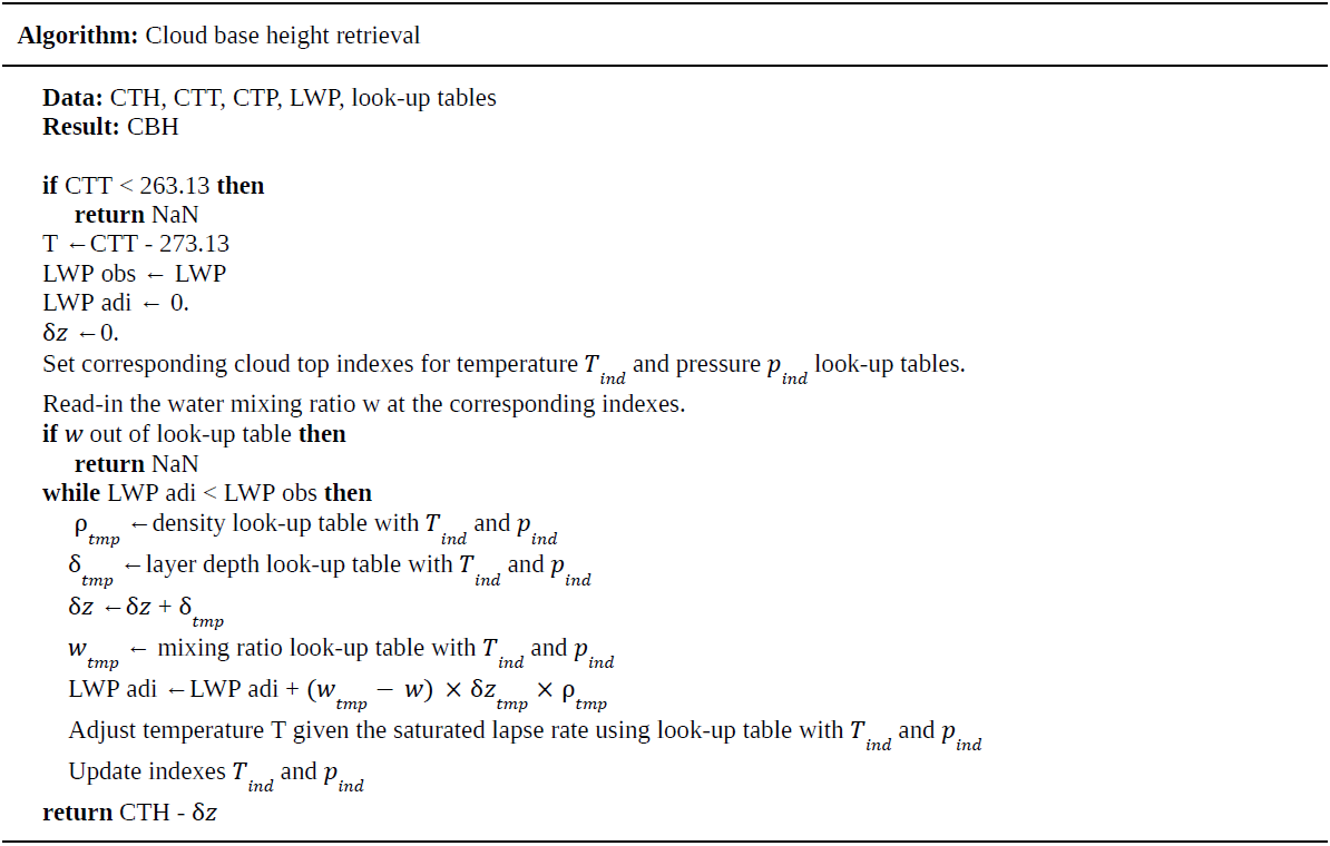
The algorithm shown below is adapted from Goren et al. (2018). We use the retrieved CTH, CTT, CTP, and CWP from MODIS MYD06 (Platnick et al., 2017). Pseudo code for cloud base height retrieval algorithm assuming adiabatic cloud, adapted from Goren et al. (2018).