Quantifying particulate matter optical properties and flow rate in industrial stack plumes from the PRISMA hyperspectral imager

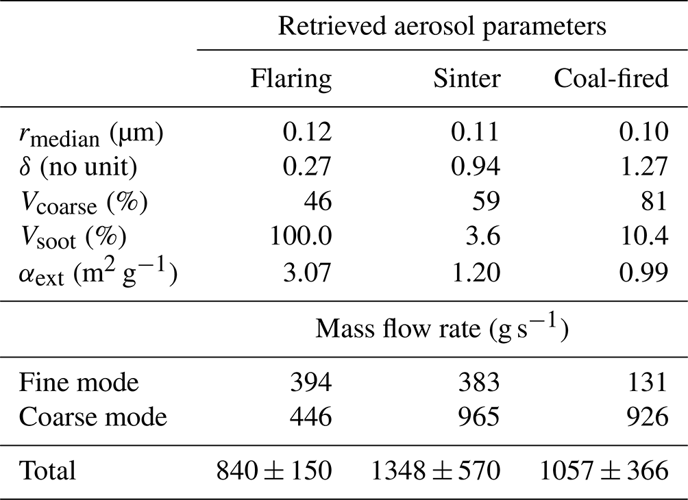
Industrial activities such as metallurgy, coal and oil combustion, cement production, and petrochemistry release aerosol particles into the atmosphere. We propose analyzing the aerosol composition of plumes emitted by different industrial stacks using PRISMA (PRecursore IperSpettrale della Missione Applicativa) satellite hyperspectral observations. Three industrial sites have been observed: a coal-fired power plant in Matla, South Africa (imaged on 25 September 2021); a steel plant in Wuhan, China (24 March 2021); and gas flaring at an oil extraction site in Hassi Messaoud, Algeria (9 July 2021). Below-plume surface reflectances are constrained using a combination of PRISMA and Sentinel-2/MSI images. Radiative transfer simulations are performed for each scene including the surface, background atmosphere, and plume optical properties. The plume aerosol optical thickness (AOT), particle radius, volume of coarse-mode aerosol, and soot are then retrieved within the plumes following an optimal estimation framework. The mean plume retrieved AOT at 500 nm ranges between 0.27 and 1.27 and the median radius between 0.10 and 0.12 µm. We found a volume fraction of soot of 3.6 % and 10.4 % in the sinter plant and coal-fired plant plumes, respectively. The mass flow rate of particulate matter at a point source estimated by an integrated mass enhancement method varies from 840 ± 155 g s⁻¹ for the flaring emission to 1348 ± 570 g s⁻¹ at the coal-fired plant.

1 Introduction

Industrial activities such as metallurgy, coal and oil combustion, cement production, and petrochemistry release aerosol particles into the atmosphere. The size and chemical composition of the particles vary according to the combustion or industrial processes. Fine particles emitted by coal-fired plants (Huang et al., 2017; Saarnio et al., 2014; Linnik et al., 2019; Zhang et al., 2004) or steel factories (Oravisjärvi et al., 2003; Mbengue et al., 2017; Dall'Osto et al., 2008; Weitkamp et al., 2005; Tsai et al., 2007) are generally enriched in heavy metals. Fine particles are also composed of inorganic matter such as sulfate, nitrate, and chloride (Riffault et al., 2015; Brock et al., 2003) as well as PAH or various organics emitted during incomplete combustion (Leoni et al., 2016). The aforementioned toxic elements released by industries or power plants cause adverse heath effects (Pope and Dockery, 2006; Pope et al., 2015; Brook et al., 2010; Bagate et al., 2006) and damage to the environment (Minkina et al., 2020). Regulations on industrial emissions have led to a reduction in emissions (e.g., Directive 2010/75/EU). However, emissions standards and the degree to which they are enforced vary geographically among both high- and low- to medium-income countries. Although monitoring networks dedicated to the survey of particulate matter atmospheric concentrations exist, the geographical coverage of such networks also varies geographically.

The operational monitoring of aerosol emissions by stationary industrial point sources can benefit from satellite imagery. Heavy industries often use stacks to emit and disperse hot air, particulate matter, and gaseous pollutants into the atmosphere that form visible plumes. Stack plumes can be observed from space using a dedicated VIS-SWIR camera; however, the retrieval of their aerosol content and properties remains a challenge. Retrieval algorithms (Calassou et al., 2021; Philippets et al., 2018; Foucher et al., 2019) have been developed for the characterization of industrial stack plumes using airborne VIS-SWIR hyperspectral imagery. The method proposed by Calassou et al. (2021) relies on an optimal estimation method (Rodgers, 2000) for estimating the plume aerosol optical depth and aerosol modal radius. The algorithm introduces the use of Sentinel-2/MSI VIS-SWIR images in order to evaluate the surface reflectance. In this paper, we propose applying this methodology to PRISMA (PRecursore IperSpettrale della Missione Applicativa) hyperspectral acquisitions over selected industrial emitters around the world.

The selected industrial sites are presented in the following section along with a literature review of the aerosol properties that could be expected in their stack plumes. We analyze the ability of the proposed methodology to detect the aerosol plume associated with stack emission and to retrieve the aerosol optical properties within the plume. The estimation of the particulate mass flow rate emitted by the stacks is also analyzed.

2 Selection of point-source industrial sites

2.1 Coal-fired power plant

Coal-fired plants emit a mixture of different sizes of aerosol particles. Particles emitted from coal combustion are formed by primary emission (without phase change) and through nucleation, condensation, and coagulation of vaporized species (Ninomiya et al., 2004; Saarnio et al., 2014). Ash formed during pulverized coal combustion has a bimodal size distribution (Wu et al., 1999) resulting from different formation processes and influenced by char composition (Baxter, 1992; Kleinhans et al., 2018). Several clean-up techniques (e.g., electrostatic precipitator or wet flue gas desulfurization) are implemented at the facility level in order to mitigate toxic and particulate matter emissions (Bhanarkar et al., 2008). The implementation of mitigation techniques differs according to national regulations (Xu et al., 2016). Early airborne measurements of the aerosol size distribution within the plume of coal-fired plants (Cantrell and Whitby, 1978; Richards et al., 1981) showed nuclei smaller than 0.03 µm, an accumulation mode between 0.1 and 1.0 µm, and a coarse mode between 2.0 and 7.0 µm mainly composed of fly ash. Ehrlich et al. (2007) have found a coarse mode between 6 and 7 µm, while recent observations in smokestack plumes of coal-fired plants in South Korea (Shin et al., 2022) indicate a coarse mode of particles having a diameter between 2.25 and 4.50 µm. Shin et al. (2022) and Ehrlich et al. (2007) have observed an accumulation mode with an aerodynamic diameter of 0.6 µm and geometrical standard deviation of 1.3. The mass fraction of the fine-mode aerosol is between 48 % and 62 % (Saarnio et al., 2014; Ehrlich et al., 2007). The aerosol fine fraction emitted by coal-fired plants is mainly composed of water-soluble species like SO${}_{\mathrm{4}}^{\mathrm{2}-}$ (21  %) and Ca (26  %) (Saarnio et al., 2014).

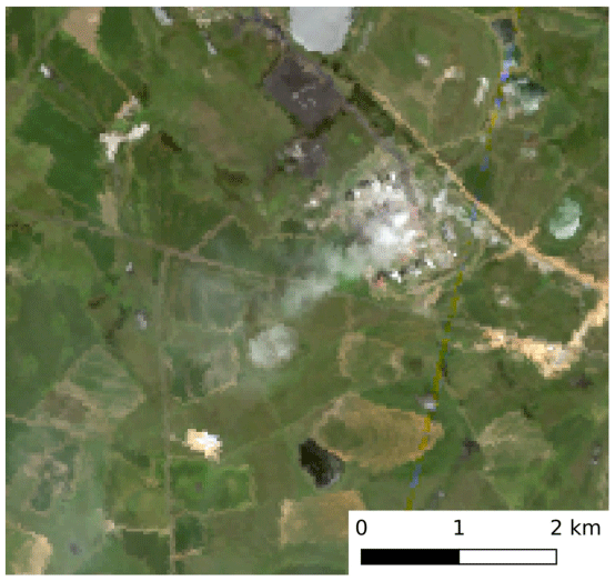
The power station of Matla (26^∘16^′52.8^′′ S, 29^∘8^′29.4^′′ E) is located at Kriel, Mpumalanga, South Africa. The power station owned by ESKOM has an installed capacity of 6 × 600 MW units. Planned retirement is between 2030 and 2034. The PRISMA image acquired on 12 February 2022 over Matla (Fig. 1) shows a distinct aerosol plume advected over a vegetated area following a N–E axis.

Figure 1 PRISMA acquisition over Matla power station on 12 February 2022.

2.2 Sinter plant

An iron and steel producing site is a complex of related plants that emit both stack and fugitive particulate matter. The sintering process is a major source of particulate matter and heavy metals. A sinter plant emits particles that are greater in quantity and finer in particle size than other steelmaking emissions (Abreu et al., 2015). Particles are composed of SO${}_{\mathrm{2}}^{-\mathrm{4}}$, NO₃, Na, K, Mg, Ca²⁺, NH${}_{\mathrm{4}}^{+}$, and trace metals (Almeida et al., 2015; Sylvestre et al., 2017). The chemical profile of particles emitted by a sinter stack is enriched in K⁺, Cl⁻, Na, and Pb (Hleis et al., 2013). Black carbon (BC) and organic carbon are also detected in sinter stack emissions (Tsai et al., 2007; Guinot et al., 2016). Following Leoni et al. (2016) the aerosol size distribution is composed of three modes having aerodynamic diameters of 0.1, 0.6, and 6 µm. The fine-mode fraction can be estimated between 30 % and 65 % based on the PM fractions measured by Ehrlich et al. (2007) and Almeida et al. (2015).

China produces about half of the world's steel (Bo et al., 2021). The emission of air pollutants by the steel industry in China has been responsible for air quality degradation and human health problems, leading to the introduction of strengthened emission standards (Tang et al., 2020). Wuhan Iron and Steel Co., Ltd. (30^∘38^′24^′′ N, 114^∘27^′36^′′ E) is an integrated steel plant in Wuhan, Hubei province, China. Its nominal crude steel capacity is 15 910 t yr⁻¹. The factory is located in a peri-urban zone composed of residential areas and agricultural plots.

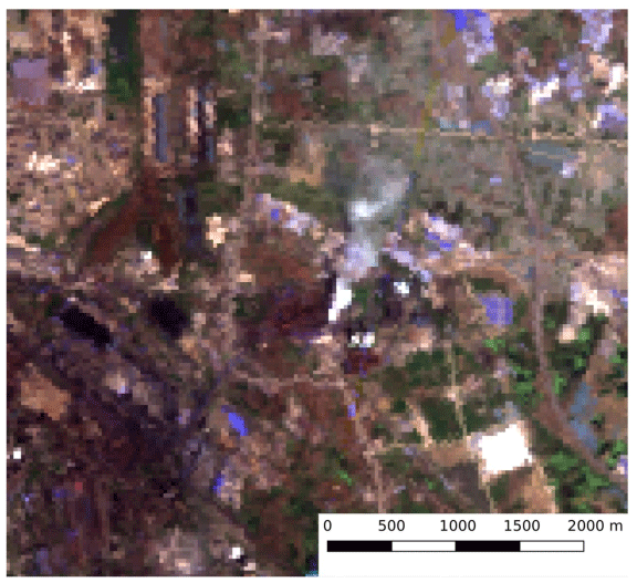
The plume observed in the PRISMA image on 24 March 2021 (Fig. 2) is located to the east of the steelmaking industry and moves northeastward. The landscape is heterogeneous, being a mix of residential housing and fields.

Figure 2 PRISMA acquisition over Wuhan (China) on 24 March 2021.

2.3 Oil flaring

Flaring is the act of burning off excess gas from oil wells. Flaring happens for economical reasons when excess gas cannot be stored and is sent elsewhere or for security reasons. Flaring from oil wells (also called upstream flaring or flaring of associated gas) is a significant source of greenhouse gases, aerosol particles, and precursors of particles (Klimont et al., 2017).

The incomplete combustion of the flared gas produces soot consisting of mass-fractal-like aggregates of BC containing nanoscale spherules (Fung, 1990). The associated emission factor for BC ranges between 0.13 g m⁻³ (Schwarz et al., 2015; Weyant et al., 2016) and 1.6 g m⁻³ of gas flared (Stohl et al., 2013). Flared gas volumes in terms of methane equivalent are globally estimated using the method proposed by Elvidge et al. (2016) and based on VIIRS flare detection (Elvidge et al., 2013). However, the BC emission factor can vary significantly between different oil and gas fields (Huang and Fu, 2016). BC strongly absorbs visible light (Bond and Bergstrom, 2006; Bond et al., 2013). Its density is estimated between 1.7 g m⁻³ (Kondo et al., 2011) and 1.9 g cm⁻³ (Medalia and Richards, 1972; Janzen, 1980). The diameter of soot particles emitted by flaring ranges between 10 and 200 nm and most commonly lies between 10 and 50 nm (Fawole et al., 2016).

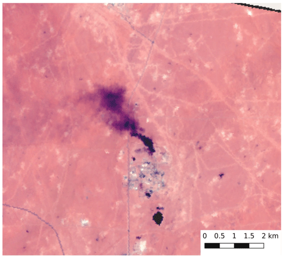
Hassi Messaoud oil field (31^∘80^′ N, 6^∘5^′ E) is located in Ouargla province in Algeria. Its production is 56 000 m³ d⁻¹. Hassi Messaoud is a hotspot of gas flaring in the world and an anomalous point source of methane (Lauvaux et al., 2022; Guanter et al., 2021; Varon et al., 2021). A PRISMA image was acquired on 9 July 2021 at 11:00 LT showing three distinct plumes, two located south of the main city and one in the north. The plumes are easily detectable due to the high contrast between the dark smoke and the bright reflective desertic landscape. The northern plume (Fig. 3) has a northwest orientation, a length of 3 km, and an area of 2 km². This plume is emitted by four flares.

Figure 3 PRISMA acquisition over Hassi Messaoud (Algeria) on 9 July 2021.

3 Retrieval process

3.1 Satellite data and pre-processing

The PRISMA mission was launched in March 2019 by the Italian Space Agency for a duration of 5 years. The standard size of a single image is 30 × 30 km with a ground sampling distance of 30 m. PRISMA is flying a Sun-synchronous low-Earth orbit at an altitude of 615 km with a local time of Equator crossing on descending node at 10:30 LT (Cogliati et al., 2021). The hyperspectral imaging spectrometer on board PRISMA covers the nominal 400–2500 nm spectral range with a sampling interval between 11 and 15 nm. PRISMA hyperspectral data have been used to detect methane plumes and to quantify methane emission due to oil extraction (Guanter et al., 2021) and carbon dioxide emission by power plants (Cusworth et al., 2021).

The aim of the pre-processing is to estimate the surface reflectance below the aerosol plume by using a combination of multispectral SENTINEL-2(S2)/MSI and hyperspectral PRISMA observations. S2/MSI observations are acquired with a few days of delay from PRISMA acquisitions. S2/MSI images were acquired on 27 June and 23 March 2021 as well as 20 February 2022 at 11:00 LT for the flaring, sinter plant, and coal-fired plant study cases, respectively. S2/MSI has 13 spectral bands between 0.4 and 2.2 µm. The pixel resolution is between 10 and 60 m depending on the channel. Both PRISMA and S2/MSI images are first corrected from background atmospheric effects using COCHISE software (Miesch et al., 2005), a front end of MODTRAN software. The atmospheric parameters used for the atmospheric correction are the ones provided by the ESA along with the S2/MSI images (Main-Knorn et al., 2017). The co-registration between the two images is operated by using an optical flow algorithm named GEFOLKI (Brigot et al., 2016). The hyperspectral reflectances below the plume in the PRISMA image are inferred from the out-of-plume PRISMA reflectances and the S2/MSI images using the coupled non-negative matrix factorization (CNMF) technique (Yokoya et al., 2012). CNMF estimates the hyperspectral surface reflectances below the plume as a linear combination of hyperspectral end-members weighted by the S2/MSI reflectances. The hyperspectral end-members are extracted from the hyperspectral image by a vertex composite analysis (VCA) unmixing method (Nascimento and Dias, 2005).

3.2 Direct model

The signal measured by a satellite sensor is usually expressed in radiance (W sr⁻¹ µm⁻¹ m²). For a flat, homogeneous, and Lambertian ground in a configuration where the environmental effects are neglected, the measured signal can be decomposed as

$$\begin{array}{}\text{(1)}& L_{\mathrm{tot}}=L_{\mathrm{atm}}+\mathit{\rho }{\displaystyle \frac{(E_{\mathrm{d}}+E_{\mathrm{s}})(T_{\mathrm{d}}+T_{\mathrm{s}})}{\mathit{\pi }(\mathrm{1}-\mathit{\rho }S)}},\end{array}$$

where L_atm is the atmospheric radiance, i.e., the radiance without interaction with the ground; E_d and E_s are respectively the direct and scattering part of the solar irradiance; T_d and T_s are the direct and scattering parts of the atmospheric transmittance; ρ is the surface reflectance; and S is the spherical albedo of the atmosphere (Kaufman et al., 1997; Vermote et al., 1997; Liou, 2002). For convenience, we normalize the solar illumination by converting the top-of-atmosphere (TOA) radiance L_tot into a TOA reflectance signal ρ_TOA. The conversion from radiance to TOA reflectance is performed by using the following equation:

$$\begin{array}{}\text{(2)}& {\mathit{\rho }}_{\mathrm{TOA}}={\displaystyle \frac{\mathit{\pi }{L}_{\mathrm{tot}}}{E_{\mathrm{TOA}}{\mathit{\mu }}_{\mathrm{s}}}},\end{array}$$

where E_TOA represents the TOA solar irradiance and μ_s is the cosine of the azimuth solar angle. In the presence of a plume, all the radiative terms except the surface reflectance ρ are affected.

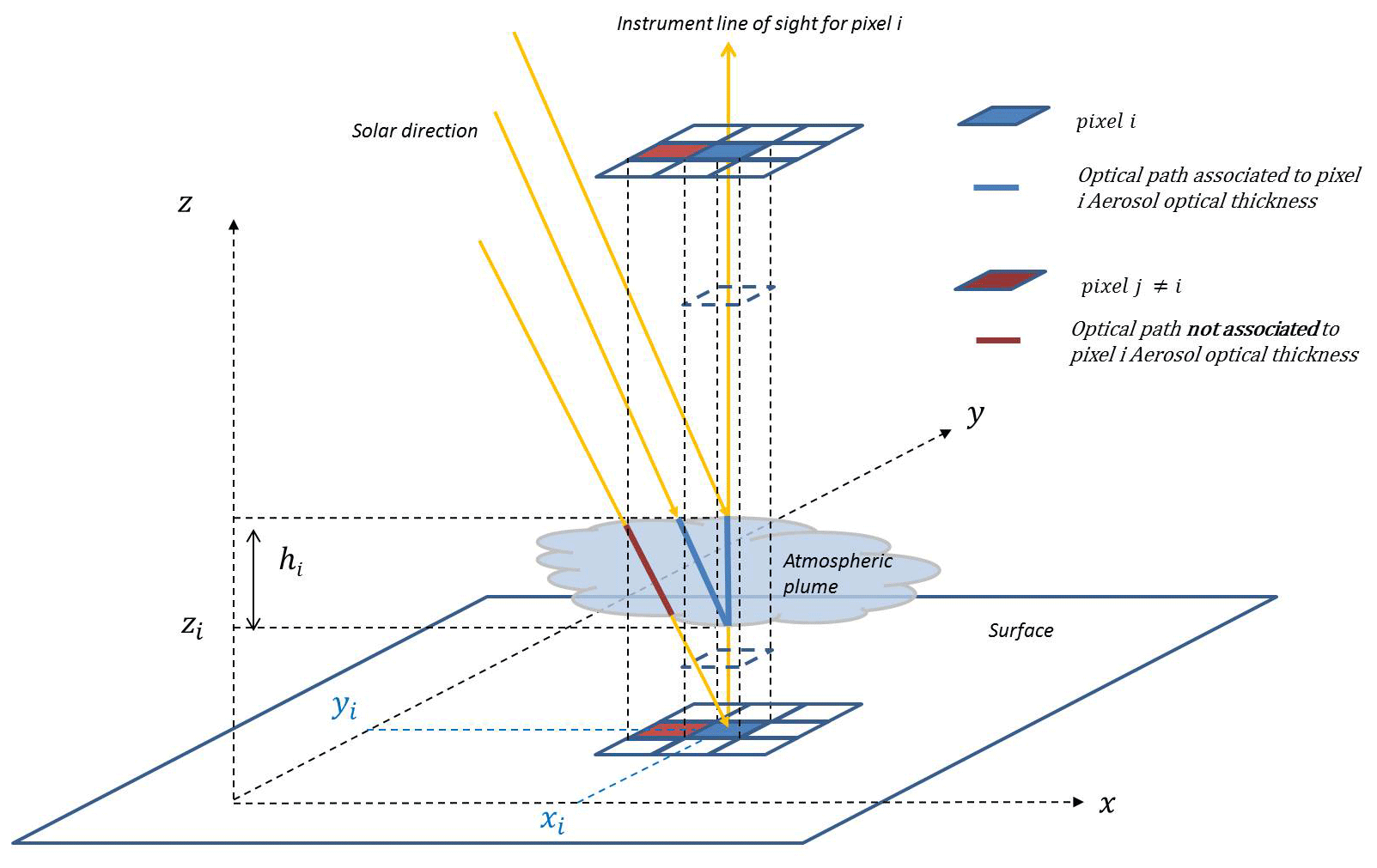
Figure 4 Schematic representation of the interaction of solar radiation with a particle plume emitted by a stack.

The direct model associated with pixel i for a spectro-imager is based on the COMANCHE software (Miesch et al., 2005) for the calculation of the different terms L_atm, E_d, E_s, T_d, T_s, and S under a plane and parallel atmospheric hypothesis. A first calculation is done corresponding to the atmospheric conditions of the acquisition, and then a second calculation is necessary to introduce the aerosol plume radiative impact. To avoid a complex 3D atmospheric model while taking into account the spatial heterogeneity of the plume concentration, we introduce a dual-AOT model. The dual-AOT model for a nadir viewing angle is illustrated in Fig. 4. Besides the AOT associated with pixel i for the upward irradiance denoted as δ, a second AOT is denoted as δ^∗ for the downward irradiance intercepting the pixel i surface at the ground level. The optical paths for δ and δ^∗ are illustrated in Fig. 4 by the blue and red lines, respectively. Thus δ^∗ does not correspond to the pixel i atmospheric column as illustrated in Fig. 4. Depending on the geometry of the plume (height, thickness, and direction) and the solar position, δ^∗ can take very heterogeneous values: low values for pixels at the edge of the plume when the downward flux does not intercept the plume, values close to δ (pixels at the heart of a fairly extensive plume), or high values at the edge of the plume when the downward flux crosses the plume at its heart. The final direct model for a pixel of coordinates (x_i,y_i) with corresponding AOT δ is

$$\begin{array}{}\text{(3)}& L_{\mathrm{tot}}=L_{\mathrm{atm}}^{\mathit{\delta }}+\mathit{\rho }{\displaystyle \frac{\left(E_{\mathrm{d}}^{{\mathit{\delta }}^{\ast }}+E_{\mathrm{s}}^{\mathit{\delta }}\right)\left(T_{\mathrm{d}}^{\mathit{\delta }}+T_{\mathrm{s}}^{\mathit{\delta }}\right)}{\mathit{\pi }(\mathrm{1}-\mathit{\rho }S)}},\end{array}$$

where X^δ means a calculation of X including a plume-homogeneous plane-parallel layer associated with the AOT value δ.

Our assumption is that these two parameters can be estimated independently using only the radiance observed at pixel i at sensor level: δ is associated with the extinction and scattering (reflection) properties of the plume, while δ^∗ is only associated with the extinction properties of the aerosol plume.

3.3 Optimal estimation formalism

The optimal estimation method (OEM) is a regularized matrix inverse method based on Bayes' theorem (Rodgers, 2000). The measured spectral radiance vector y is modeled as a vector-valued function:

$$\begin{array}{}\text{(4)}& \mathit{y}=F\left(\mathit{x}\right)+\mathit{ϵ},\end{array}$$

where F is the forward model, ϵ the modeling noise, and x the state vector. The forward model F accounts for the atmosphere, instrument, surface, and plume aerosol properties.

The optimal estimation uses an iterative approach that minimizes a cost function χ given by

$$\begin{array}{}\text{(5)}& \mathit{\chi }=(\mathit{x}-{\mathit{x}}_{\mathrm{a}}{)}^T{\mathbf{S}}_{\mathrm{a}}^{-\mathrm{1}}(\mathit{x}-{\mathit{x}}_{\mathrm{a}})+(\mathit{y}-\mathbf{K}\mathit{x}{)}^T{\mathbf{S}}_{\mathit{ϵ}}^{-\mathrm{1}}(\mathit{y}-\mathbf{K}\mathit{x}).\end{array}$$

The Jacobian matrix of the problem K is built using a look-up table (LUT) of radiative transfer simulations calculated with MODTRAN (Berk et al., 2014) at each iteration. The state vector is limited to the aerosol plume parameters and composed of the AOTs at 550 nm (δ₅₅₀ and ${\mathit{\delta }}_{\mathrm{550}}^{\ast }$), the median radius of the accumulation mode (r_median), the volume proportion of the coarse mode in the size distribution (V_coarse), and the volume proportion of carbonaceous particles in the accumulation mode (V_soot). Associated with each parameter of x, a prior distribution is given by the state vector x_a and the prior uncertainties in the variance–covariance matrix S_a.

The matrix S_ϵ contains both the measurement uncertainties S_y and the uncertainties of the model parameters that are not retrieved, S_b. S_b includes the different uncertainties due to (i) the reconstruction of the surface reflectances under the plume with the CNMF, (ii) the water vapor concentration in the atmosphere, and (iii) the background aerosol visibility. The uncertainties coming from the surface reflectances are obtained by calculating the spatial standard deviation for each wavelength of the hyperspectral spectrum for pixels outside the spatial footprint of the plume (firstly visually identified). The uncertainties due to the water vapor concentration and the background aerosol visibility are empirically fixed based on a literature review of hyperspectral instrument retrievals (Bhatia et al., 2018; Rodger, 2011; Yang et al., 2017). For water vapor, the uncertainties can be as low as a few percent but a more realistic 10 % is retained. The uncertainty of the background aerosol visibility is set to 5 km. The uncertainties of the unknown in the model b are projected on the state space by approximating these uncertainties to the first order thanks to K_b, the Jacobian matrix containing the partial derivatives associated with these parameters. The observation uncertainties is given by

$$\begin{array}{}\text{(6)}& {\mathbf{S}}_{\mathit{ϵ}}={\mathbf{S}}_y+{\mathbf{K}}_b^T{\mathbf{S}}_b^{-\mathrm{1}}{\mathbf{K}}_b.\end{array}$$

The cost function χ is minimized using the Levenberg–Marquardt (LM) algorithm. At each iteration the state vector x_i is updated by

$$\begin{array}{}\text{(7)}& \begin{array}{rl}{\mathit{x}}_{i+\mathrm{1}}& ={\mathit{x}}_i+{\left({\mathbf{K}}^T{\mathbf{S}}_{\mathit{ϵ}}^{-\mathrm{1}}\mathbf{K}+{\mathbf{S}}_{\mathrm{a}}^{-\mathrm{1}}\times (\mathrm{1}+\mathit{\gamma })\right)}^{-\mathrm{1}}\\ & \times \left[{\mathbf{K}}^T{\mathbf{S}}_{\mathit{ϵ}}^{-\mathrm{1}}\mathbf{K}(\mathit{y}-\mathbf{K}\mathit{x})+{\mathbf{S}}_{\mathrm{a}}^{-\mathrm{1}}(\mathit{x}-{\mathit{x}}_{\mathrm{a}})\right],\end{array}\end{array}$$

where γ is a regularization term allowing us to adjust the step size of the LM algorithm.

The uncertainties associated with the posterior state vector $\widehat{\mathit{x}}$ are contained in the variance–covariance matrix $\widehat{\mathbf{S}}$ given by

$$\begin{array}{}\text{(8)}& \widehat{\mathbf{S}}={\left({\mathbf{S}}_{\mathrm{a}}^{-\mathrm{1}}+{\mathbf{K}}^T{\mathbf{S}}_{\mathit{ϵ}}^{-\mathrm{1}}\mathbf{K}\right)}^{-\mathrm{1}}.\end{array}$$

The averaging kernel matrix is used for the purpose of error analysis. The averaging kernel matrix A can be defined analytically as the product of the Jacobian matrix K and the gain matrix G.

$$\begin{array}{}\text{(9)}& \mathbf{G}={\left({\mathbf{K}}^T{\mathbf{S}}_{\mathit{ϵ}}^{-\mathrm{1}}+{\mathbf{S}}_{\mathrm{a}}^{-\mathrm{1}}\right)}^{-\mathrm{1}}{\mathbf{K}}^T{\mathbf{S}}_{\mathit{ϵ}}^{-\mathrm{1}}\end{array}$$

The different terms of A can also be defined as the partial derivative $\partial \widehat{\mathit{x}}/\partial {\mathit{x}}^{\ast }$ representing the variation of the posterior state vector $\widehat{\mathit{x}}$ with respect to the changes in the true state x^∗. The diagonal elements of A are the degrees of freedom (DOF) of the retrieved parameter. DOFs evaluate the independence of each restitution from the prior constraint and range between 0 (totally dependent on the prior vector) and 1 (totally dependent on the measurements).

3.4 Aerosol models

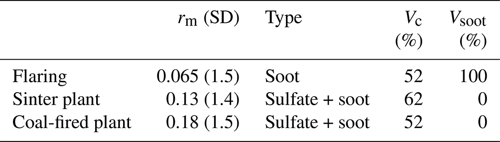
The size distribution of the aerosol models is bimodal and includes an accumulation (fine) and a coarse mode. The refractive index of the accumulation mode is defined as an internal mixture between the refractive index of a scattering (sulfate) and an absorbing aerosol (soot) from the OPAC database (Hess et al., 1998). Prior information for the aerosol models is given in Table 1. The prior aerosol models and associated uncertainties are established following the literature review presented in Sect. 2. The literature review proposes a range of aerodynamic diameters for the accumulation modes and partial information on the width of the size distribution. The aerodynamic diameter is set to 0.22, 0.67, and 0.60 µm for the flaring, sinter plan, and coal-fired plant respectively. The coarse mode for the sinter and coal-fired emissions is simulated as a dust-like non-spherical aerosol using an axis ratio of 2 (Mishchenko et al., 1997; Dubovik et al., 2002). The physical radius of the coarse mode is set to 0.5 µm (standard deviation of 2.0). The aerosol optical properties are simulated using the MOPSMAP T-matrix algorithm (Gasteiger and Wiegner, 2018). Prior estimate of the coarse-mode fraction is based on reported particulate mass fraction. For flaring emission, as there is no reported value for V_c, we have fixed the prior value to the one of the coal-fired plant.

Table 1 Prior information on fine-mode aerosol median radius r_m, model type, and volume fraction V_c. SD is the standard deviation of the lognormal mode.

The simulated atmosphere contains a stack plume having a thickness of 100 m (Leoni et al., 2016) and a base at 50 m above the ground. The plume height is defined empirically; however, it has a negligible impact on the forward model simulations. The direct simulations are performed at the spectral resolution of PRISMA for the ranges 420 to 870, 1000 to 1090, 1190 to 1290, 1530 to 1710, and 2080 to 2400 nm.

3.5 Retrieval of mass flow rate

The pixel-by-pixel columnar mass density ΔΩ (in g m⁻²) of the plume is given as the ratio between δ and the mass extinction efficiency α_ext (Hand and Malm, 2007). α_ext (at 550 nm wavelength) is a function of the retrieved aerosol model parameters given by the state vector x.

The uncertainties in ΔΩ are estimated using the posterior uncertainties in δ and α_ext. ΔΩ is then used to estimate the mass flow rate at the point source. The different methods developed to estimate the mass flow rate from satellite imagery can be classified in four families: inversion methods using Gaussian plumes (Bovensmann et al., 2010), so-called source pixel methods (Jacob et al., 2016), cross-sectional methods also called cross-sectional flux methods (Tratt et al., 2011, 2014; Krings et al., 2011, 2013), and the integrated mass enhancement method (Varon et al., 2018, 2021; Frankenberg et al., 2016). The integrated mass enhancement (IME) method overcomes the shortcomings of the previously presented methods with respect to the configuration of the studied data, i.e., a plume image for which knowledge of the wind comes from large-mesh meteorological data and for which the stability of the atmosphere is unknown to us. IME for a given pixel j of area A_j is given by

$$\begin{array}{}\text{(10)}& \mathrm{IME}=\sum _{j=\mathrm{1}}^N\mathrm{\Delta }{\mathrm{\Omega }}_j{A}_j.\end{array}$$

The mass flow rate Q (in g s⁻¹) is the ratio between the IME and a characteristic residence time of the particles in the detected plume. The residence time can be expressed as the ratio between an effective wind speed U_eff and a characteristic length of the plume L (Frankenberg et al., 2016; Varon et al., 2018), leading to

$$\begin{array}{}\text{(11)}& Q={\displaystyle \frac{U_{\mathrm{eff}}}{L}}\times \mathrm{IME}.\end{array}$$

As stated by Varon et al. (2018), U_eff and L must be viewed as operational parameters to be related to the observed wind speed and plume extent. The definition of L will influence the relationship between U_eff and the 10 m wind. L is usually defined as equal to the square root of the area of the detected pixels. In the case of a constant direction of propagation over time, L can be chosen as equal to the length of a study area in the plume propagation direction and U_eff as an average wind speed. In this configuration, the IME calculation is equivalent to the calculation of an average cross-sectional flux.

The flow rate uncertainties δQ are estimated using the relative uncertainties in U_eff and ΔΩ. U_eff and its relative error are estimated from the ensemble model of ERA5 reanalysis.

4 Retrieval of aerosol optical properties in industrial stack plumes

4.1 Gas flaring

In the case of the Hassi Messaoud gas flare, the surface reflectances are easily reconstructed by CNMF due to a homogeneous ground surface. Moreover, the high contrast between the plume and the ground favors the detection of the plume.

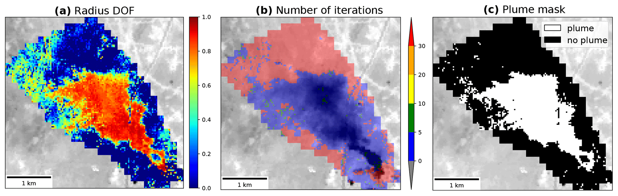
Figure 5 OEM results on the flaring plume: (a) median radius DOF, (b) number of iterations in the LM algorithm, and (c) combined mask.

The DOFs associated with the retrieved AOT and median radius, as well as the number of iterations in the LM algorithm, are used to detect the spatial footprint of the plume. The DOF on the AOT is equal to 0.99 on average and the values are spatially homogeneous in the plume. Applying a threshold of 0.5 to the median radius DOF (Fig. 5a) highlights the footprint of the plume, except near the source. The mask obtained with DOF > 0.5 keeps the pixels whose retrievals are more than 50 % independent of the prior constraint.

The number of iterations of the LM algorithm also gives a good proxy for the plume footprint. The visual comparison between the color composition (Fig. 3) and the number of iterations of LM algorithm (Fig. 5b) indicates that most of the plume is found within 10 iterations. We note that at the source level, the LM algorithm does not converge, probably due to the flame thermal emission. Indeed, the temperature of this flame is estimated to be 1750 K according to SkyTruth (https://skytruth.org/flaring/, last access: 21 December 2023) and leads to a significant emission in the SWIR that is not accounted for in our model. The masks given by DOF > 0.5 and the number of iterations < 10 are combined (multiplied by each other) to give a plume mask (Fig. 5c). The resulting plume detection corresponds well to the visual inspection of the corresponding color composition (Fig. 3).

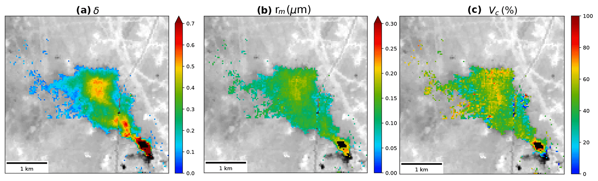
Figure 6 Estimation of (a) aerosol optical thickness at 550 nm, (b) fine-mode median radius, and (c) coarse-mode fraction in the flaring plume.

The AOT is a component of the state vector in the optimal estimation procedure. Its value is retrieved by minimizing the cost function that integrates the look-up tables computed using the direct radiative transfer model and the aerosol optical properties (Sect. 3.3 and 3.4). The initial value of AOT is set to 0.5 with an uncertainty of 1.0. The retrieved AOT map (Fig. 6a) reflects the plume structure and shows several maxima in the plume near the point source and downwind. The mean plume AOT is equal to 0.27 (see summary Table 3), which is associated with a mean statistical uncertainty equal to 0.011.

Some artifacts that are due to CNMF reconstruction are located near the road and correspond to sandy structures that have moved between the PRISMA and S2/MSI acquisitions.

The retrieved radii (Fig. 6b) are rather homogeneous with a spatial variation of 0.03 µm and on average equal to 0.12 µm with a statistical uncertainty of 0.02 µm. The final V_c (Fig. 6c) converges to 46 % with a spatial standard deviation of 13 %.

4.2 Sinter plant

Plume delineation for the sinter and coal-fired plants follows the same procedure based on DOF and iteration number as explained for the gas flaring case (Sect. 4.1). In the case of the sinter plant, one must pay attention to the geometry of illumination of the scene. Indeed, we can observe in Fig. 2 that the plume propagation direction is 20^∘ with respect to the geographical north. The solar azimuth angle θ_s is 144^∘. So the angular difference between the direction of illumination of the Sun and the direction of the plume is 56^∘. For a plume having a vertical extent of ≈ 500 m, the distance between the crossing points of the downward flux and the upward flux is almost equal to the widest part of the plume. Consequently, an additional AOT associated with E_d (see Sect. 3.2 and discussion section hereafter) is also retrieved. Moreover, a variable fraction of soot particles in the accumulation mode (volume fraction V_soot) is introduced in the state vector to better fit the aerosol hyperspectral signal.

The ascending part of the plume appears, as in the case of Hassi Messaoud, to be the densest (Fig. 7). The plume puffs are perceptible through AOT local maxima.

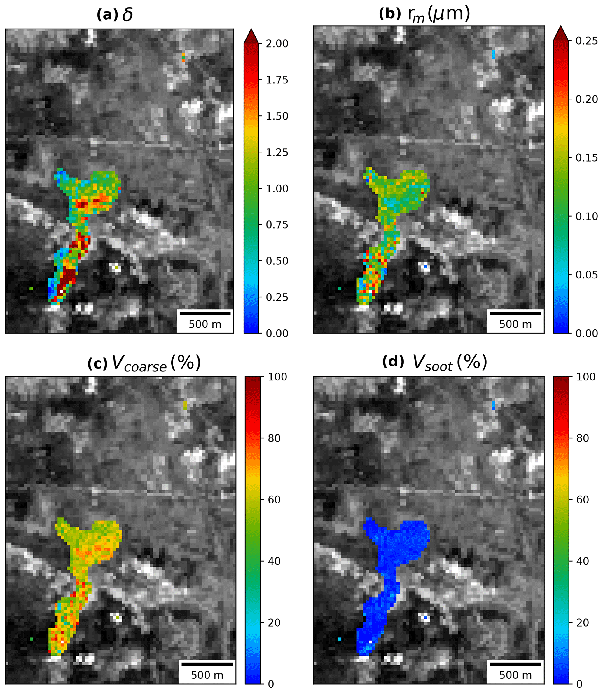
Figure 7 Estimation of (a) aerosol optical thickness at 550 nm, (b) fine-mode median radius, (c) coarse-mode fraction, and (d) volume of soot in the sinter plant plume.

Finally, the other retrieved parameters of the state vector are spatially homogeneous. The median radius of the accumulation mode is on average equal to 0.11 ± 0.02 µm in the pixels present in the plume mask. The statistical uncertainties associated with these radii are equal to 0.05 µm. The volume proportion of the coarse mode is 59 % (with a statistical uncertainty of 14 %), being 20 % higher than the measurements found in the literature.

4.3 Coal-fired plant

For the coal-fired plant case study, the plume mask detection fails to recover the entire plume (Fig. 8). Only the densest part of the plume near the source and another area of vegetation with dark and homogeneous surface reflectances (Fig. 8) are identified. The partial detection can be due to a poor reconstruction of the vegetated soils in the visible part of the spectrum because of the growth of the vegetation between the PRISMA and S2/MSI images (8 d). For every pixel where the surface reconstruction error is high there is a low sensitivity to aerosol optical depth. So optically thin plumes (AOT below 0.7) cannot be detected.

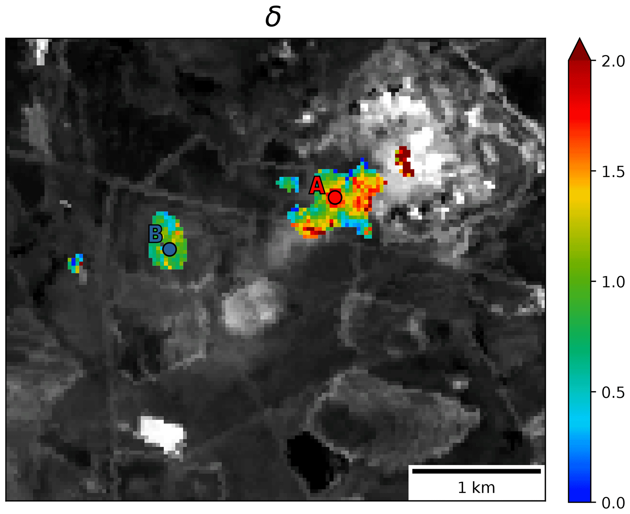
Figure 8 Optical thickness map at 550 nm obtained from the OEM. A local study of the OEM retrievals is performed at points A and B.

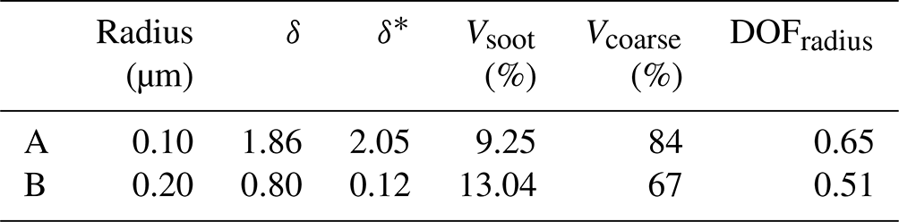
To illustrate the variability in the retrieval conditions, we have selected two areas of 3 × 3 pixels in each detected zone (A and B in Fig. 8). Point A is located in a dense part of the plume, while point B is located downwind. Both points are located over vegetated areas. Retrieved AOT at point A is 1.8, while it is 0.8 further downwind at point B (see Table 2). The sensitivity of the retrieval model to the spectral variations induced by the different physical parameters is proportional to the particle concentration in the plume. We first observe that the degrees of freedom associated with the radius are higher for point A (0.65) than for point B (0.51), indicating that the point B retrieved radius is more strongly constrained by its prior information than at point A. The aerosol radius at point B is equal to 0.20 µm, which is relatively close to the prior value, while the retrieved radius for point A is equal to 0.10 µm. Finally, it is interesting to note that the retrieved AOT associated with the descending solar flux (δ^∗) is much lower at point B than point A due to its shifted position with respect to the propagation axis of the plume.

Table 2 Aerosol optical parameters in the coal-fired plant plume at selected locations A and B (see Fig. 8).

5 Mass flow rate

The surface mass concentration ΔΩ (Fig. 9) is estimated using the retrieved AOT and the mass extinction efficiency (see Sect. 3.5). The detection limit (borders of the plumes) is around 0.1 g m⁻². The surface mass concentration is up to 2 g m⁻² in the case of the coal-fired plant plume. The surface mass calculated in the densest areas of plumes corresponds to an atmospheric concentration between 1 and about 10 mg m⁻³ for a plume vertical extent of 100 m. The mass flow rate is estimated in selected parts of the plumes after visual inspection (red rectangles in Fig. 9). The selected areas are outside the rising part of the plume. The effective wind speed U_eff is equal to 7, 3, and 2 m s⁻¹ for the flaring emission, sinter plant, and coal-fired plant, respectively. The flow rate is split into the fine- and coarse-mode components (Table 3). The total estimated flow rate varies from 840 g s⁻¹ for the flaring emission to 1348 g s⁻¹ for the coal-fired plant emission. The uncertainties are discussed in the section below (Sect. 6.1).

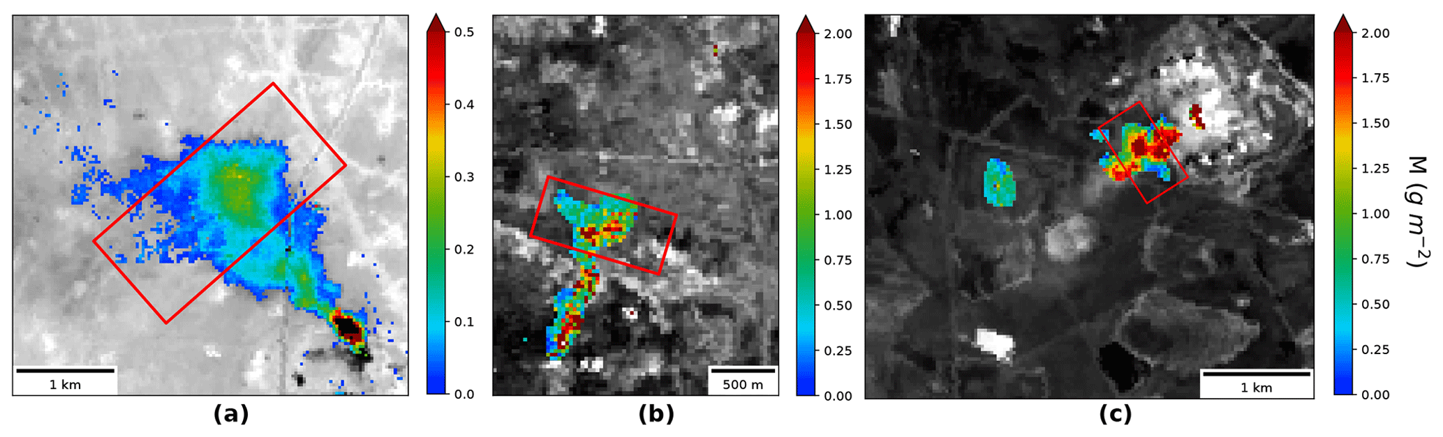
Figure 9 Plume surface mass (in g m⁻²) retrieved for (a) flaring emission, (b) sinter plant emission, and (c) coal-fired plant emission. Red rectangles are the selected area for mass flow rate estimation.

Table 3 Average retrieved plume aerosol properties.The aerosol optical thickness δ and the mass extinction efficiency α_ext are given at 550 nm.

6 Discussion

6.1 Uncertainty analysis

The surface reflectance reconstruction below the plume is affected by (i) the co-registration process, (ii) the time lag between PRISMA and S2/MSI acquisitions, and (iii) the end-members used for the CNMF. For heterogeneous scenes, like the sinter plant and the coal-fired plant, the end-members are less representative than for homogeneous scenes like the flaring site. Although the surface reflectances are high around the flaring site (≈ 0.1), the associated error is 2 times lower than for the other two studied cases (Fig. 10). The relative error in the surface reflectance reaches 60 % at 500 nm in the case of the coal-fired plant (Fig. 10). The vegetation growth between the PRISMA and S2/MSI acquisition in the case of the coal-fired plant might be responsible for such a drastic impact on the reflectance reconstruction.

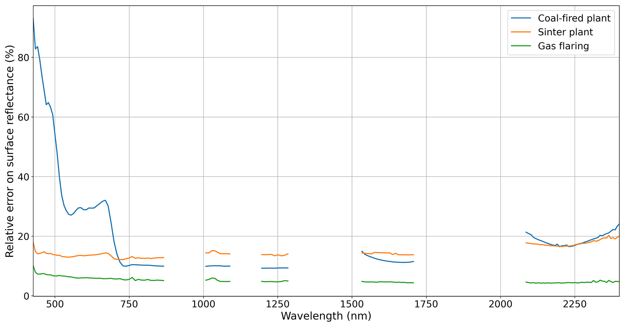
Figure 10 Relative error in the surface reflectance reconstruction for the flaring site (green), sinter plant (orange), and coal-fired plant (blue).

The errors associated with the surface reflectance estimation and the aerosol property retrieval process (given by the matrix $\widehat{\mathbf{S}}$ in Eq. 8) are used to estimate the uncertainties in the plume surface mass estimate. The surface mass uncertainties (δΔΩ) are estimated by using the uncertainties in the AOT (hereinafter δ(AOT)) and the mass extinction efficiency (δα_ext).

$$\begin{array}{}\text{(12)}& \mathit{\delta }\mathrm{\Delta }\mathrm{\Omega }=\sqrt{{\left({\displaystyle \frac{\mathit{\delta }\left(\mathrm{AOT}\right)}{\mathrm{AOT}}}\right)}^{\mathrm{2}}+{\left({\displaystyle \frac{\mathit{\delta }{\mathit{\alpha }}_{\mathrm{ext}}}{{\mathit{\alpha }}_{\mathrm{ext}}}}\right)}^{\mathrm{2}}}\times \mathrm{\Delta }\mathrm{\Omega }\end{array}$$

and δα_ext can be decomposed into

$$\begin{array}{}\text{(13)}& \mathit{\delta }{\mathit{\alpha }}_{\mathrm{ext}}=\sqrt{\sum _{i=\mathrm{1}}^n{\left({\displaystyle \frac{\partial {\mathit{\alpha }}_{\mathrm{ext}}}{\partial {\widehat{\mathit{x}}}_i}}\right)}^{\mathrm{2}}{\widehat{\mathbf{S}}}_{i,i}}\times {\mathit{\alpha }}_{\mathrm{ext}},\end{array}$$

where i represents the values of all the parameters of the posterior state vector $\widehat{\mathit{x}}$ except AOT and ${\widehat{\mathbf{S}}}_{i,i}$ the variances of each of these parameters present on the diagonal of the variance–covariance matrix $\widehat{\mathbf{S}}$. The $\widehat{\mathbf{S}}$ matrix also contains the surface reflectance CNMF error. The estimated uncertainties in the retrieved parameters are given in Table 4.

Table 4 Uncertainties in the retrieved aerosol parameters.

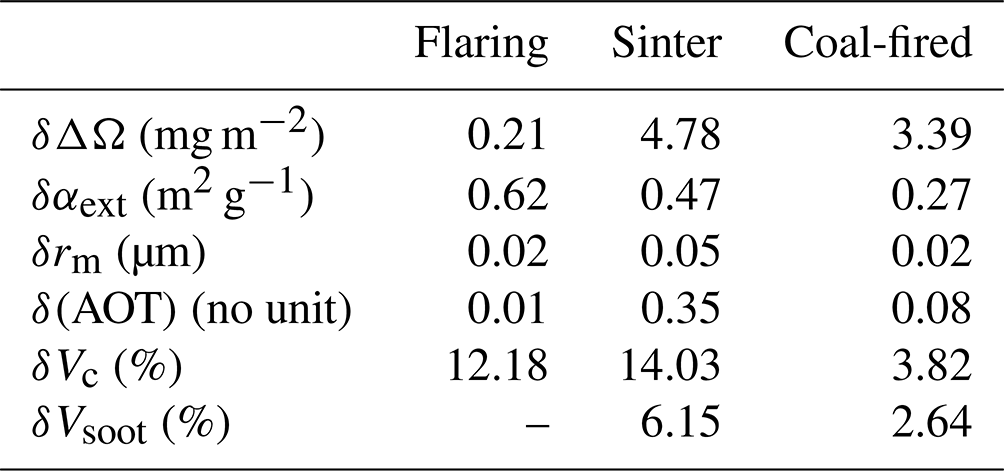
The contribution of the error in the retrieved parameters to the surface mass uncertainty depends on the case study. When the surface reflectances are poorly reconstructed (sinter and coal-fired plant) the AOT error contribution is around 40 %, while the contribution is 7 % for the flaring site (Table 5). However, the error associated with the retrieval of the coarse-mode fraction in the case of the flaring emission drastically impacts the error in the surface mass concentration (75 %). The error associated with the estimation of the soot fraction in the accumulation mode has a rather weak impact on the final error in the surface mass concentration. Indeed the soot fraction is rather low (see Table 3) for the sinter and coal-fired plant plumes.

Table 5 Relative contribution (in %) of parameter uncertainty to the surface mass variance and to the flow rate variance.

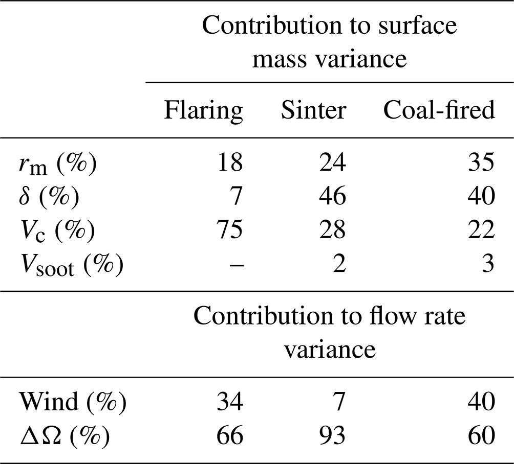
The error in the flow rate is due to the cumulative error in the effective wind speed and the surface mass concentration (see Table 5, bottom part). The wind uncertainties are equal to 1, 0.5, and 0.5 m s⁻¹ for the flaring emission, the sinter, and coal-fired plant, respectively. The wind speed uncertainty represents a substantial contribution to flow rate variance, which could be decreased thanks to better knowledge of local atmospheric conditions. In the case of the sinter plant, the variance in the flow rate estimate is still largely dominated by the large error in the surface mass concentration (see Table 4). The uncertainties in the total mass flow rate, given the uncertainties in the surface mass concentration and the effective wind speed, are estimated to be 155, 570, and 366 g s⁻¹ for the gas flaring, sinter plant, and coal-fired plant, respectively (also reported in Table 3).

Another source of error in the estimation of the flow rate comes from the definition of U_eff in the IME method. The relationship between U_eff and the 10 m wind speed depends on the measurement condition, the method used to estimate the flow rate, and the instrument specifications (Varon et al., 2018). Based on large-eddy simulations for methane plumes, an underestimation of the actual flow rate by 30 % to 50 % can be expected (Nesme et al., 2021; Varon et al., 2021).

6.2 Concentration and flow rate

As we have selected remarkable plumes, the flow rates must be seen as top estimations. The total flow rate calculated for each site is in the upper range of expected values, being about 1 kg s⁻¹. The sites are large-scale facilities in countries having legislation less restrictive than European standards. For the Hassi Messaoud flaring site, the flares emit 0.10 billion cubic meters (BCM) of gas in 2021 according to SkyTruth. Applying the emission factor of Caseiro et al. (2020), the corresponding annual emission of fine particles is 10⁸ g. Assuming that these flares emit continuously over the year, the average flow rate associated with a flare is 3 g s⁻¹. The fine-mode flow rate associated with one flare is 98.5 g s⁻¹ (the plume is generated by four flares), being about 2 orders of magnitude greater than the average flow rate. By analyzing 130 images of S2-A and S2-B over Hassi Messaoud for which the flares were visible, we have detected only five plumes having the same size or even larger. Consequently, the case study of Hassi Messaoud is probably an uncommon phenomenon.

The impact on the air quality in the surrounding area of the facilities will drastically depend on the ventilation of the plume and how it vertically disperses. The detection limit of 0.1 g m⁻² for the visible plume corresponds to an atmospheric concentration of 200 µg m⁻³ for a plume vertical extent of 500 m. The atmospheric concentration is about 1 order of magnitude above the 50 µg m⁻³ limit of EU Directive 2008/50/EC that must not be exceeded more than 35 times during a calendar year. Although the proposed method is not dedicated to the monitoring of air quality around the facilities, high-spatial-resolution observations of plume transport can provide unique information for understanding the impact of industrial emissions. The main limitation for an operational survey of plume emissions is the reduced number of observations due to cloud occurrence and the revisit time of the satellite.

7 Conclusion

We propose an inversion framework to retrieve instantaneous particulate matter emission by industrial stacks using hyperspectral PRISMA satellite images. Aerosol plume satellite retrieval over continental surfaces is a challenge, and we had to implement different steps to unravel the impact of the underlying surface and the impact of the particle size, concentration, and type on the satellite signal. At first, the fusion algorithm with operational S2/MSI images provided an estimate of the surface reflectance and its uncertainties below the plume. The radiative impact of the plume on a background atmosphere was then simulated for varying plume particle median radius, aerosol optical thickness, and volume proportion of soot also considering the geometrical conditions of the scene. The uncertainties associated with the surface reflectance estimation were propagated to the final aerosol solution using the OEM formalism. The use of OEM allows retrieving a plume mask and the associated aerosol properties. Setting up the prior aerosol model for each type of emission was achieved based on a review of available but scarce literature. The inversion was tested over three types of industries: a coal-fired plant, a sinter plant, and an oil flaring site. In most of the cases the entire plume area could not be investigated and the mass flow rate was estimated by selecting limited portions of the plume. Moreover, the relationship between the actual wind speed and IME effective wind speed would have required further investigations considering the uncertainties in the retrieved surface mass as well as the plume dynamic. Nevertheless, the retrieved aerosol physical characteristics and the estimated instantaneous emission flow rate are within the expected range for each type of emission.

The synergy between PRISMA and S2/MSI could be improved in several ways. Using a time series of S2/MSI rather than the nearest image in time could improve the estimation of the surface reflectance variability. Moreover, the aerosol model as retrieved using the hyperspectral imager could be prescribed to S2/MSI with the aim of providing regular acquisition of the plume time evolution. Lastly, going down to a 10 m spatial resolution could improve the detection of narrow plumes provided that the surface is rather homogeneous.

A comprehensive validation exercise of the retrieved parameters would require in situ measurement of the mass float rate by aerosol size fraction, aerosol size distribution, and chemical composition within the plume as well as the plume extent. However, due to the large difficulties of accessing industrial infrastructures, the validation of the retrieved mass flow rate or aerosol properties remains virtually impossible for our case studies. At least a consistency check could be performed between soot emission by flares based on the stack emission temperature and the retrieved soot flow rate. And as a perspective, the use of high-spatial-resolution satellites for aerosol retrievals over industrial sites is also promising for the improvement of top-down emission inventories as the number of hyper spectral satellite missions is expected to increase in the near future.