Supercooled liquid water cloud classification using lidar backscatter peak properties

The use of depolarization lidar to measure atmospheric volume depolarization ratio (VDR) is a common technique to classify cloud phase (liquid or ice). Previous work using a machine learning framework, applied to peak properties derived from co-polarized attenuated backscatter data, has been demonstrated to effectively detect supercooled-liquid-water-containing clouds (SLCCs). However, the training data from Davis Station, Antarctica, include no warm liquid water clouds (WLWCs), potentially limiting the model's accuracy in regions where WLWCs are present. In this work, we apply the same framework used on the Davis data to a 9-month micro-pulse lidar dataset collected in Ōtautahi / Christchurch, Aotearoa / New Zealand, a location which includes WLWC. We then evaluate the results relative to a reference VDR cloud-phase mask. We found that the Davis model performed relatively poorly at detecting SLCC with a recall score of 0.18, often misclassifying WLWC as SLCC. The performance of our new model, trained using data from Ōtautahi / Christchurch, displays recall scores as high as 0.88 for identification of SLCC, although it generally underestimates SLCC occurrence. The overall performance of the new model highlights the effectiveness of the machine learning technique when appropriate training data relevant to the location are used.

1 Introduction

Supercooled liquid water (SLW) droplets exist in clouds at temperatures below 0 °C and above the homogeneous nucleation freezing temperature of around −40 °C (e.g. DeMott and Rogers, 1990; Khain and Pinsky, 2018). Heterogeneous nucleation of ice in clouds occurs at temperatures between −40 and 0 °C when SLW droplets interact with ice-nucleating particles (INPs), such as dust and other aerosols, or other ice particles (Hoose and Möhler, 2012). Regions in which INPs are scarce thus favour increased quantities of SLW clouds (Murray et al., 2012), hereafter referred to as SLWCs. In mixed-phase clouds (MPCs) between −40 and 0 °C, SLW droplets and ice particles are both present. In this study, we use the term “supercooled-liquid-water-containing clouds” (SLCCs) to refer to clouds that may be either mixed-phase or composed solely of supercooled liquid water droplets.

Previous work has shown that SLWCs and MPCs are common over the Southern Hemisphere, particularly the Southern Ocean, using satellite (Hogan et al., 2004; Hu et al., 2010; Morrison et al., 2011; Huang et al., 2012) and in situ observations (Chubb et al., 2013) and that these clouds are underrepresented in numerical weather prediction (NWP) (Forbes and Ahlgrimm, 2014) and climate models (Mason et al., 2015; Schuddeboom and McDonald, 2021). This uncertainty in cloud occurrence and cloud phase has a large impact on models' radiation budgets (Bodas-Salcedo et al., 2016; Vergara-Temprado et al., 2018). When SLWCs are underrepresented in models, too much sunlight warms the Southern Ocean instead of being reflected from cloud tops back to space, causing an artificial heating of the sea surface. This is the main contributor to sea surface temperature (SST) biases observed in many CMIP5 models (Hyder et al., 2018). Understanding the formation processes of SLWC is therefore an important topic of research to reduce biases in the radiation budget in NWP and global climate models over the Southern Hemisphere.

Moreover, accurate satellite-based classification of cloud phase is generally limited to regions near cloud top (Blanchard et al., 2014; Protat et al., 2014). Recent work has shown that satellites underestimate low-altitude SLWC due to attenuation from higher-altitude clouds (Liu et al., 2017; Alexander and Protat, 2018; McErlich et al., 2021). Therefore, while satellite-based measurements allow for global analysis of high-altitude SLWC occurrence, ground-based remote sensing observations are essential for accurate measurement of low-level clouds that are imperfectly measured from space.

Lidar is an active remote sensing technique that involves the transmission of laser pulses into the atmosphere and the measurement of returned radiation backscatter from liquid drops, ice crystals, aerosols and other atmospheric constituents (Emeis, 2011). In this study we use a micro-pulse lidar (MPL), which has a depolarization capability that allows for the calculation of the linear volume depolarization ratio δ, hereafter referred to as VDR, as calculated in Eq. (1). This value includes contributions from both particle and molecular backscatter within a volume and differs from the linear particle depolarization ratio (Lewis et al., 2020). The utility of the VDR to determine cloud phase was first identified by Schotland et al. (1971), and it has been used in numerous studies since to classify liquid water and ice-phase clouds (Sassen, 1991; Lewis et al., 2020; Ricaud et al., 2024). The difference in VDR between liquid and ice clouds occurs because spherically symmetric liquid water droplets produce little to no depolarization, whereas backscatter from complex ice crystals tends to be depolarized and thus have higher VDR. Various studies have derived different thresholds to distinguish liquid- and ice-phase cloud, but most agree that δ<0.1 is characteristic of liquid water clouds, with δ>0.4 for ice clouds and intermediate values representing mixed-phase clouds (Sassen, 1991). It should be noted, however, that horizontally aligned ice crystals can produce specular reflections and decreased values of VDR, meaning such clouds can be misclassified as liquid. This is usually mitigated by orienting the lidar off-zenith (Hogan and Illingworth, 2003). Furthermore, multiple scattering from multiple layers of liquid clouds can sometimes cause cross-polarized reflection and thus higher VDR, causing some liquid clouds to be falsely classified as ice.

Ceilometers are simpler automatic lidars that do not have depolarization capability and only measure the co-polarized lidar backscatter. A methodology to detect SLCC from ceilometers, using only co-polarized backscatter, would allow SLCC occurrence to be analysed using widely used existing ceilometer networks, negating the need for polarized lidar systems. Moreover, application to historical datasets would allow cloud-phase retrievals to be extended to past records. Previous work by Hogan and Illingworth (1999) proposed a method of SLCC detection using ceilometers, and further studies developed new algorithms (Hogan et al., 2003; Hogan and O’Connor, 2004; Tuononen et al., 2019) for scientific and operational usage. Operational networks of comprehensive observing systems, such as the Atmospheric Radiation Measurement (ARM) Climate Research Facility (Mather and Voyles, 2013) and Cloudnet (Illingworth et al., 2007), use synergistic radar–lidar algorithms to retrieve cloud properties including cloud phase. Within the Cloudnet retrieval, liquid water detection is based on empirically derived thresholds of lidar attenuated backscatter (Hogan et al., 2003; Illingworth et al., 2007) and, in recent versions, the attenuated backscatter profile shape (Tuononen et al., 2019; Tukiainen et al., 2020).

More recently, Guyot et al. (2022) implemented a machine learning classification model applied to lidar observations collected at Davis Station, Antarctica, and found that it outperformed the technique of Tuononen et al. (2019). A reference cloud-phase mask was created from a merged depolarization lidar and W-band cloud radar product and used to train an extreme gradient boosting (XGBoost) model (Chen and Guestrin, 2016) with single-polarization ceilometer backscatter peak properties. The model was named G22-Davis to reflect the fact that the training data were from Davis. Guyot et al. (2022) found that G22-Davis outperformed previous methods of SLCC detection, with accuracy scores as high as 0.91 compared to 0.84 for the application of the Tuononen et al. (2019) approach. However, a key consideration is that at Davis, virtually all liquid water will be in the supercooled state. No warm liquid water was detected over a year-long period based on ceilometer observations and the G22-Davis retrieval at Davis (Guyot et al., 2022). It is therefore important to determine whether the G22-Davis model can be applied to mid-latitude and lower-latitude sites, where “warm” liquid water clouds with temperatures greater than 0 °C exist. Furthermore, for the G22-Davis technique to be practical for wider use, it should be evaluated in a variety of conditions and regions. This provides the central motivation for this study. The aims of this study are to (i) evaluate the performance of G22-Davis for our dataset of MPL observations from Ōtautahi / Christchurch, Aotearoa / New Zealand (henceforth Christchurch); (ii) using the same methodology (Guyot et al., 2022), develop a new model for SLWC identification trained using Christchurch MPL measurements; and (iii) apply the resulting cloud-phase masks to produce a climatology of SLWC for Christchurch.

2 Datasets and methodology

2.1 Datasets

2.1.1 Christchurch MPL observation campaign

For the Christchurch field campaign, a Droplet Measurement Technologies mini-micro-pulse lidar (MPL) was installed and operated from May 2021 to January 2022 on the roof of the Ernest Rutherford building on the University of Canterbury campus (43.5225° S, 172.5841° E) at an altitude of 45 m. The MPL is a compact dual-polarization elastic backscatter lidar that operates at a wavelength of 532 nm and has a range of 30 km. For the Christchurch deployment, the vertical range resolution was set to 15 m, and the averaging time was set to 30 s. The minimum range and detection height of the MPL are 100 m. The scanning head of the MPL enclosure was set to a fixed vertical scanning mode with elevation angle 90°.

Post-processing of the raw MPL data is completed with version 1.2.1 of the Automatic Lidar and Ceilometer Framework (ALCF), a software package detailed in Kuma et al. (2021b). While individual ceilometers typically implement post-processing in their firmware, ALCF provides a consistent noise reduction and calibration method that can be applied to different ceilometer types, and it has been applied in previous studies using ceilometer datasets in Antarctica (Guyot et al., 2022) and the Southern Ocean (Kuma et al., 2020; Kremser et al., 2021; Pei et al., 2023). First, raw MPL data were converted with the mpl2nc tool (Kuma, 2020), which performs after-pulse, overlap and dead-time calibration and calculates cross- and co-polarized normalized relative backscatter (NRB) from cross- and co-polarized raw backscatter counts. ALCF performs noise reduction, absolute calibration and cloud detection from the mpl2nc-derived NRB, including resampling of the data to a common 5 min temporal and 50 m vertical resolution. More details on ALCF methodologies are provided by Kuma et al. (2021b).

2.1.2 AMPS

The Antarctic Mesoscale Prediction System (AMPS) is a real-time limited-area numerical weather prediction (NWP) system based on the Polar Weather Research and Forecasting (Polar WRF) model (Powers et al., 2012; Hines and Bromwich, 2008). The AMPS forecasting system is used for scientific and logistical purposes in Antarctica and is extended to cover New Zealand because of Christchurch's status as an Antarctic gateway city, providing access to Scott Base and McMurdo Station. The AMPS NZ grid has a 6 km spatial resolution on 21 pressure levels, available in 3-hourly intervals initialized at 00:00 and 12:00 UTC. Real-time forecasts are available online in GRIB1 format and were set to automatically download during the study period and convert to NetCDF (NC). Due to occasional download errors, AMPS data were not available for 29 d of the 9-month study period. Temperature data were extracted for the nearest-neighbour grid cell corresponding to the University of Canterbury site. The two-dimensional time × pressure-level temperature field was cubic-spline-interpolated to a finer grid size, and the hydrostatic balance equation, assuming an isothermal atmosphere, was applied to resample to a 2 d time × altitude grid to match the resolution of the ALCF-derived products. Isotherms at 0 and −40 °C were also determined from the Polar WRF output.

2.2 Cloud-phase masks

ALCF performs cloud detection using an attenuated volume backscatter coefficient threshold algorithm (Kuma et al., 2021b). The cloud mask was determined to be positive where the attenuated volume backscatter coefficient was greater than a tunable threshold plus 5 standard deviations of noise. The default backscatter threshold for ALCF of $\mathrm{2}\times {\mathrm{10}}^{-\mathrm{6}}{\mathrm{m}}^{-\mathrm{1}}{\mathrm{sr}}^{-\mathrm{1}}$ was used during preliminary analysis of the Christchurch MPL dataset but was found to be too low and resulted in a significant number of false positive detections in the lowest 1 km, likely due to the presence of boundary layer aerosols. This is likely due to ALCF being tuned for usage over the nearly pristine aerosol environment of the Southern Ocean (Bhatti et al., 2023). Instead, a backscatter threshold of $\mathrm{4}\times {\mathrm{10}}^{-\mathrm{6}}{\mathrm{m}}^{-\mathrm{1}}{\mathrm{sr}}^{-\mathrm{1}}$ was chosen as a good compromise between boundary layer aerosol false positives and high-altitude cirrus false negatives based on visual inspection. The ALCF cloud mask product was used as the starting point of the depolarization ratio reference mask.

2.2.1 MPL depolarization ratio reference mask

Several previous studies to determine cloud phase from polarized lidar backscatter retrievals used the linear volume depolarization ratio, VDR (Sassen, 1991; Lewis et al., 2020). The principle is described in Sect. 1. For the cloud-phase reference mask used in this study, we apply an algorithm similar to the one described by Lewis et al. (2020) for MPL measurements. In the first step, mpl2nc-derived cross-polar P_cross and co-polar P_co normalized relative backscatter (NRB) profiles are regridded by averaging to match the resolution of the ALCF and Polar WRF products. VDR δ at altitude z was calculated by

$$\begin{array}{}\text{(1)}& \mathit{\delta }\left(z\right)={\displaystyle \frac{P_{\mathrm{cross}}\left(z\right)}{P_{\mathrm{co}}\left(z\right)}}\end{array}$$

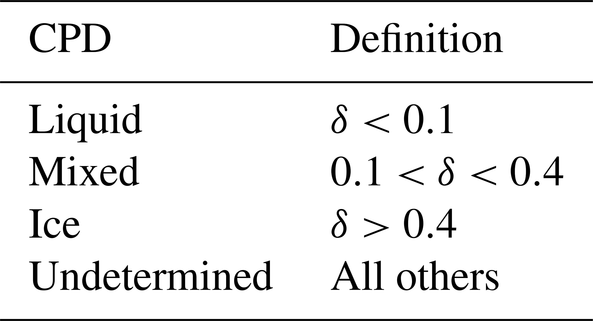
for each bin in the detected cloud layer. Then, VDR was used to assign a cloud-phase diagnostic (CPD), representing the likely cloud phase for each altitude bin, as defined in Table 1. The thresholds to define liquid, mixed-phase and ice were chosen following a sensitivity test on the values of VDR from all cloud bins in the dataset. The cumulative frequencies of VDR, as a function of temperature, are shown in Fig. 1. For warm bins (above 0 °C and therefore nearly all liquid), Fig. 1 shows that most bins have δ<0.1. For bins in the mixed-phase temperature regime (−40 to 0 °C), VDR increases with decreasing temperature. This is due to the increased presence of ice at colder temperatures and the corresponding increase in VDR. For bins less than the homogeneous freezing value (−40 °C) VDR is much higher and nearly always δ>0.4. Therefore, thresholds of 0.1 and 0.4 were chosen to distinguish liquid, mixed phase and ice, respectively. The phase of an entire cloud layer was assigned from the most frequent CPD of the altitude bins in that layer. Additionally, the WRF-derived temperature T for an altitude bin was used to distinguish supercooled liquid water clouds (SLWCs, T<0 °C) and warm liquid water clouds (WLWCs, T>0 °C), as well as to limit SLWC and MPC to $T>-\mathrm{40}\mathit{°}$C.

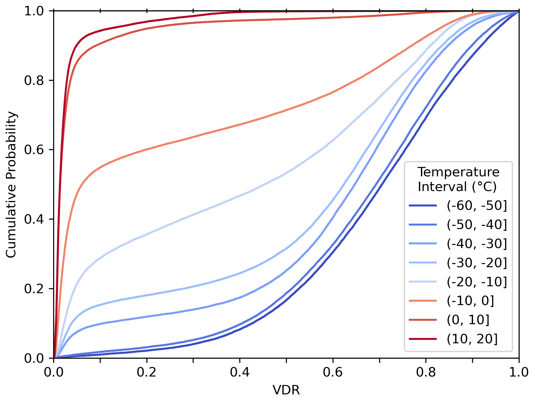
Figure 1 Empirical cumulative distribution of VDR for clouds in a range of temperature intervals.

Table 1 Cloud-phase diagnostic (CPD) determined from MPL-measured linear volume depolarization ratio δ.

2.3 Development of a data-driven cloud-phase mask

The method described here follows the process detailed in Guyot et al. (2022) to develop a data-driven model for the classification of cloud as SLCC. The first step in the Guyot et al. (2022) methodology was to extract backscatter peak properties from a single-polarization ceilometer. In our case, ALCF-derived attenuated volume backscatter coefficient β profiles from the MPL dataset were used in place of the single-polarization ceilometer backscatter profiles. Since ALCF applies consistent calibration and resampling, the expectation is that the model developed here is applicable to any calibrated lidar data processed with ALCF, using the default 50 m vertical and 5 min temporal resolution.

Each profile of attenuated volume backscatter coefficient β was analysed using the signal processing tools in the SciPy Python library (Virtanen et al., 2020) to identify peaks (local maxima). For each peak exceeding a minimum value of $\mathit{\beta }>\mathrm{2}\times {\mathrm{10}}^{-\mathrm{5}}{\mathrm{m}}^{-\mathrm{1}}{\mathrm{sr}}^{-\mathrm{1}}$ and minimum width of 50 m, a set of properties were recorded: the value of backscatter at peak location (i.e. the peak magnitude) $\mathit{\beta }\left({\mathrm{m}}^{-\mathrm{1}}{\mathrm{sr}}^{-\mathrm{1}}\right)$; peak width w (m); the peak prominence ${\mathit{\beta }}_{\mathrm{prom}}\left({\mathrm{m}}^{-\mathrm{1}}{\mathrm{sr}}^{-\mathrm{1}}\right)$ defined as the difference between the peak and its lowest contour line; the “peak width height” ${\mathit{\beta }}_{\mathrm{w}}\left({\mathrm{m}}^{-\mathrm{1}}{\mathrm{sr}}^{-\mathrm{1}}\right)$ defined as the value of backscatter where peak width is determined, calculated from ${\mathit{\beta }}_{\mathrm{w}}=\mathit{\beta }-(\mathrm{0.5}\times {\mathit{\beta }}_{\mathrm{prom}})$; the peak altitude z (m) above ground level; the total number of peaks for a given profile n; and the peak order within that total number, in the range (0,n). These peak properties are the same as those used in the original study by Guyot et al. (2022), and readers should refer to Fig. 6 in that study for an illustration of the peak characteristics. In addition to the peak properties, the WRF-derived temperature for the peak's altitude bin was also recorded. The eight-feature dataset of peak properties was then labelled with the reference mask classification of the altitude bin as SLWC, WLWC, MPC or ice cloud (IC).

Guyot et al. (2022) noted the importance of accounting for lidar extinction in multilayer situations. When multiple cloud layers are present, the returned backscatter from higher layers is weaker due to attenuation of the lidar signal from lower layers. Guyot et al. (2022) compared peak properties for primary peaks (where peak order = 0) and secondary peaks (where peak order > 0), finding a statistically significant separation between primary and secondary peak magnitudes (Guyot et al., 2022, Fig. 3). They found peak magnitude values of both primary and secondary peaks to have normal distributions and derived an offset term for direct comparison of primary and secondary peaks. This offset was calculated as the absolute difference of the distributions' medians and was $\mathrm{4.2}\times {\mathrm{10}}^{-\mathrm{5}}{\mathrm{m}}^{-\mathrm{1}}{\mathrm{sr}}^{-\mathrm{1}}$ for their dataset. This was hypothesized to be the average reduction in lidar backscatter due to extinction from the lower layer(s). For our Christchurch MPL dataset, we compared the distributions of primary and secondary peak properties, which are shown in Fig. 2. Unlike Guyot et al. (2022, Figure 3), the attenuated backscatter peak magnitude values are not normally distributed, and both skew right to greater values of peak magnitude. That is, in our dataset there are more peaks with higher values of the backscatter coefficient. This effect is more pronounced for primary peaks. This disparity with the distributions of Guyot et al. (2022, Fig. 3) could be because our dataset is significantly larger (around 30 000 vs. 3700 primary peaks and 5000 vs. 570 secondary peaks) and therefore more varied, because of an instrumental effect (e.g. due to the different wavelength of the Davis ceilometer, or a calibration difference), or due to a difference in environmental conditions (e.g. different aerosol concentrations causing more backscatter or more attenuation). The difference in the primary and secondary medians was calculated to be $\mathrm{6.7}\times {\mathrm{10}}^{-\mathrm{5}}{\mathrm{m}}^{-\mathrm{1}}{\mathrm{sr}}^{-\mathrm{1}}$ for our dataset. As shown in Fig. 2, the peak magnitude value corresponding to the maximum kernel density estimate (KDE), i.e. the mode, is the same for primary and secondary peaks, and there is significant overlap between the two distributions, unlike those in Guyot et al. (2022, Fig. 3). Therefore, we chose not to scale the magnitudes of secondary peaks by adding an offset.

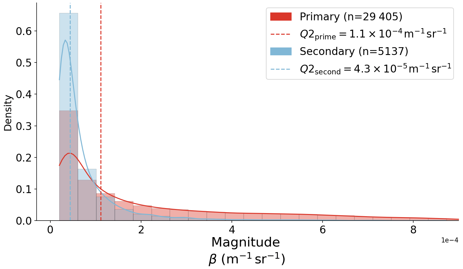
Figure 2 Histogram and kernel density estimation (KDE) plots of backscatter peak magnitudes for primary (peak order = 0) and secondary (peak order > 0) peaks. Histograms are normalized such that the bar heights sum to 1. The median of each distribution, Q2_prime and Q2_second, respectively, is also plotted.

The next step in the development of the cloud-phase mask was to train and test a data-driven model that could perform multi-class classification of each peak as SLWC, WLWC or neither. As in Guyot et al. (2022), we also chose XGBoost due to its excellent performance in a wide range of applications (Chen and Guestrin, 2016), often outperforming other decision tree or boosting model approaches. XGBoost is an optimized version of gradient tree boosting, an ensemble supervised learning algorithm. During training, XGBoost iteratively builds a series of “weak” learners (regression trees) that are fitted to minimize the loss (i.e. error) of the resulting predictor, whilst also minimizing complexity to avoid overfitting. XGBoost applies numerous performance optimization strategies when building and combining the trees, reducing computational costs and allowing it to be scalable to large datasets. The XGBoost model developed by Guyot et al. (2022) performed binary classification on each peak as SLCC or not. In this study, due to the presence of warm liquid water > 0 °C, we apply a multi-class classification of each peak as SLWC, WLWC or neither (implying the cloud is IC or MPC). The eight-feature dataset of peak properties was passed to the model for training along with the target label, which was the reference mask's classification of the peak as SLWC, WLWC, or IC and MPC. Model training and testing were performed on the entire peak dataset, excluding peaks from an evaluation subset made up of 15 randomly selected days. The training dataset contained 34 542 peaks related to clouds from 211 d, of which 23 % were labelled SLWC, 56 % were labelled WLWC, 2 % were labelled MPC and 17 % were labelled IC by the VDR reference mask. Preliminary analysis of the peak dataset is presented in Sect. 3.1.

The XGB model was developed using the Python library XGBoost (Chen and Guestrin, 2016), with data preparation, cross-validation and hyperparameter testing implemented using the scikit-learn Python library (Pedregosa et al., 2011). To prevent overfitting during hyperparameter testing, we applied 3-fold stratified-group cross-validation. In k-fold cross-validation, the model is trained k times on k train and test folds. Test folds never share the same data with other folds, allowing k independent validation scores and preventing overfitting of the model to a specific training set. In stratified k-fold cross-validation, each training and testing fold contains approximately the same proportion of each target class as the complete set. Finally, in group k-fold cross-validation, grouped data are split into train and test folds such that the same group is not represented in both the training and test set. In this case, groups were defined as the month in which the lidar measurement was made, thus creating nine groups with an approximately equal size and class ratio. This means that highly correlated neighbouring measurements are kept together in the same fold, ensuring that each train and test fold is independent. Due to the class imbalance in our peak dataset (shown in Sect. 3.1) we used the balanced accuracy (described in more detail in Sect. 2.4) as the scoring method for cross-validation and hyperparameter testing. To find the optimal XGB hyperparameter combination, an extended grid search was applied, with 3-fold stratified-group cross-validation, over a range of hyperparameters including maximum depth and learning rate (η). The depth of a regression tree is the number of splits (decisions) the tree makes before reaching a prediction. Therefore the maximum depth hyperparameter controls how large a tree can grow, with larger values potentially improving predictive performance but increasing complexity. The learning rate is the “shrinking” factor applied when trees are combined, and lower values reduce each tree's individual influence on the final prediction. Cross-validation testing scores are presented in Sect. 3.2.

The trained and tested XGB model was then used to predict the classification for all clouds in the MPL dataset. Each profile of attenuated backscatter was processed sequentially: firstly, peaks were identified and their properties recorded for the given profile. If no peaks were detected, that profile was labelled “cloud-free”. The detected peaks' properties were passed to the trained model for classification as SLWC, WLWC, or IC and MPC. Following the peak classification, the corresponding altitude bin was labelled with the model prediction along with the surrounding bins, with the lower and upper bounds defined as twice the peak width value, as per Guyot et al. (2022). Each profile was also labelled according to whether SLWC, WLWC, MPC or IC was present anywhere in the profile. We hereafter refer to our trained model as G22-Christchurch to reflect the fact that the model was trained on the Christchurch dataset. We applied the same method to create the G22-Davis cloud mask evaluated in this study for direct comparison with G22-Christchurch. Each peak was passed to the G22-Davis model for classification as SLCC or IC, since G22-Davis was trained to identify SLCC and IC (Guyot et al., 2022). For each peak classification, the corresponding altitude bin was labelled in the same process as described above.

2.4 Model performance metrics

Model testing and evaluation against the reference mask involve the comparison of two one-dimensional Boolean vectors for each class (SLWC and WLWC), representing the presence of cloud anywhere in the profile. Here we provide basic definitions and describe metrics used for model evaluation in this study, which are similar to those used by Guyot et al. (2022). A true positive (TP) is defined as a test result indicating a correct prediction of a positive classification for a given class (e.g. presence of SLWC), and a true negative (TN) is defined as a test result indicating a correct prediction of a negative classification (e.g. absence of SLWC). A false positive (FP) is a test result indicating an incorrect prediction of a positive classification (e.g. wrongly predicting the presence of SLWC) and a false negative (FN) is a test result indicating an incorrect prediction of a negative classification (e.g. incorrectly predicting the absence of SLWC).

Recall, or the true positive rate, is defined by Eq. (2) and represents the proportion of all true samples that are correctly classified as true, i.e. the ability of the classification to find all the positive samples:

$$\begin{array}{}\text{(2)}& \mathrm{recall}={\displaystyle \frac{\mathrm{TP}}{\mathrm{TP}+\mathrm{FN}}}.\end{array}$$

Precision is defined by Eq. (3) and represents the proportion of samples classified as true that are actually true, i.e. the ability of the classification not to label a negative sample as positive:

$$\begin{array}{}\text{(3)}& \mathrm{precision}={\displaystyle \frac{\mathrm{TP}}{\mathrm{TP}+\mathrm{FP}}}.\end{array}$$

For the multi-class classification we apply in this study, recall and precision scores are calculated for each class. Accuracy is defined as the fraction of correct predictions out of the total number of samples and is equivalent to the weighted mean of the recalls of each class. However, when classes are imbalanced (as they are in this study), accuracy scores can be subject to inflated performance estimates. The balanced accuracy is defined as the unweighted mean of the recall obtained on each class and is a more appropriate scoring method for imbalanced datasets when each class is equally important (Brodersen et al., 2010). In this study we primarily use balanced accuracy when describing the overall performance of the classification as well as recall and precision scores when describing the performance for each class.

3 Results

3.1 Peak properties dataset

We first present an analysis of the dataset of peak properties. The training dataset contained 34 542 peaks from 211 d, of which 23 % (8006 peaks) were labelled SLWC, 56 % (19 288 peaks) were labelled WLWC, 2 % (799 peaks) were labelled MPC, 17 % (5945 peaks) were labelled IC and 1 % (504 peaks) were labelled “undetermined” by the VDR reference mask. In Fig. 3 we show kernel density estimation (KDE) plots showing the distribution of all the peak properties, separated by the reference mask's cloud-phase classification as liquid (both SLWC and WLWC) or non-liquid (IC or MPC). In Fig. 4 we show similar KDE plots of liquid peak properties, this time separated by the reference mask's classification of these liquid peaks as SLWC or WLWC.

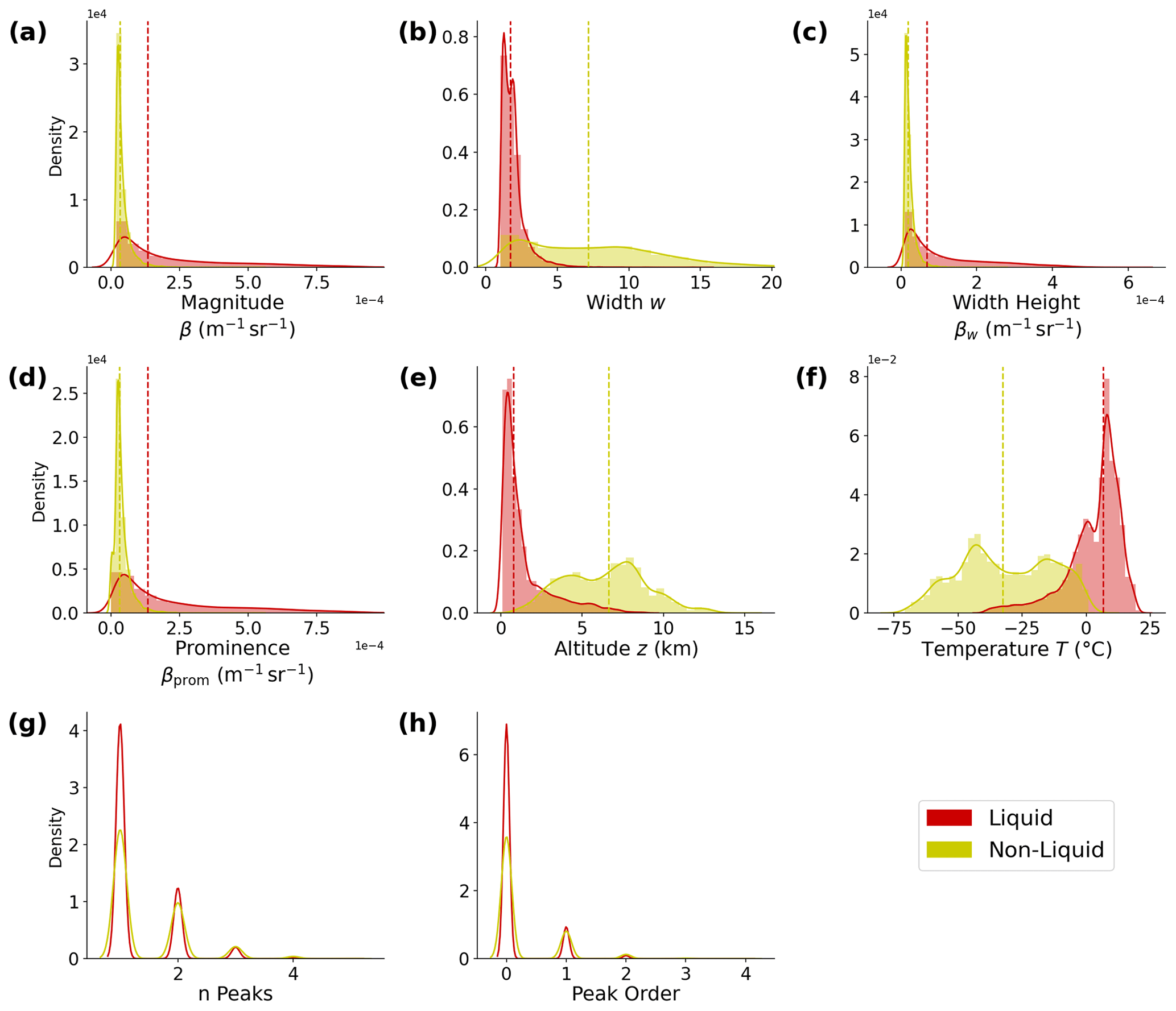
Figure 3 Kernel density estimation (KDE) plots of peak property distributions for the full dataset, with the distribution's median also plotted. Peaks are separated by the reference mask's cloud-phase classification as liquid (WLWC and SLWC) or not (IC or MPC). For n peaks and peak order (g, h), histograms and median lines are omitted for clarity. The unit for peak width is a number of range gates, which can be converted to distance by multiplying by 50 m.

Figure 3a shows that values of the backscatter peak magnitude for liquid peaks are marginally higher than those for non-liquid peaks. The same is true for peak width height (Fig. 3c) and peak prominence (Fig. 3d), which also have units of ${\mathrm{m}}^{-\mathrm{1}}{\mathrm{sr}}^{-\mathrm{1}}$ and are strongly correlated with peak height, as we show later in Fig. 8. This supports our physical understanding that liquid water is associated with stronger backscatter returned signal, as found in previous studies (Guyot et al., 2022), though clear overlap between these properties is observed in each set of distributions. It should also be noted that the difference in peak magnitude between liquid and non-liquid peaks is small, and the distributions overlap. Peak width, shown in Fig. 3b, also separates liquid and non-liquid peaks, with narrow peaks associated with liquid and wider peaks associated with IC and MPC. This is because liquid water attenuates the lidar signal more rapidly, and this attenuation is represented in the returned backscatter as a thin cloud band. The number of peaks and the peak order, which are strongly correlated, show a slight separation between liquid and non-liquid peaks, where most liquid peaks are associated with a small number (one to two) of peaks in a single profile. This agrees with the findings of Guyot et al. (2022), who found that SLWC peaks tend to be associated with single-layer cloud most frequently. This is potentially due to the attenuation effects of liquid layers that obscure higher-altitude cloud in multilayer situations.

Figure 3e shows the altitude distribution of liquid and non-liquid peaks. It shows that liquid peaks are most strongly associated with lower altitudes, with the frequency decreasing as altitude increases. The temperature distribution in Fig. 3f shows that the inverse is true of temperature: that liquid peaks are most strongly associated with warmer temperatures as we expect, and the frequency of liquid peaks decreases as temperature decreases until the lower temperature limit of around −40 °C is reached, below which homogeneous freezing occurs (DeMott and Rogers, 1990). Figure 3f shows that ice peaks are present at temperatures as low as −70 °C. Overall, the temperature distribution in Fig. 3f is representative of SLWC temperature distributions in the heterogeneous freezing temperature regime as identified in previous work (Murray et al., 2012; McErlich et al., 2021). This provides further confidence that our VDR reference mask is accurately distinguishing liquid and ice in the heterogeneous temperature range.

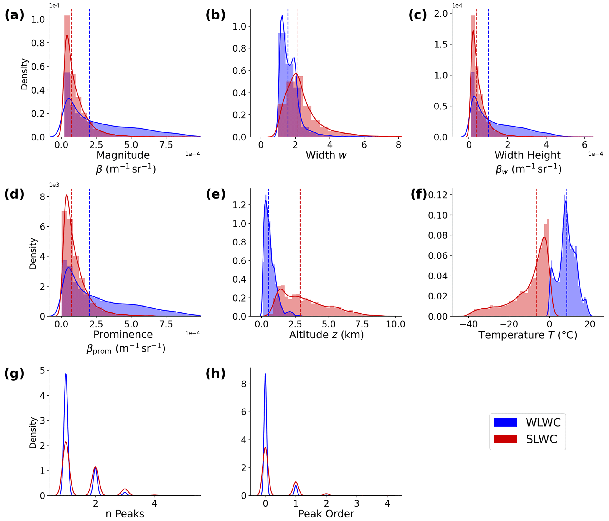
Figure 4 Kernel density estimation (KDE) plots of peak property distributions for the full dataset, with the distribution's median also plotted. Peaks are separated by the reference mask's cloud-phase classification as SLWC or WLWC. For n peaks and peak order (g, h), histograms and median lines are omitted for clarity.

Figure 4 shows the difference in average peak properties between peaks classified as SLWC and WLWC by the reference mask. Figure 4a shows that WLWC peaks generally have higher values of backscatter magnitude than SLWC peaks, and the same is true for peak width height and prominence. However, this result was found when looking at peaks from all altitudes. Given that WLWC peaks are nearly always found at altitudes below 2 km, and SLWC peaks are always found above 0.5 km (as shown in Fig. 4e), any altitude-dependent bias in attenuated volume backscatter would carry over to the SLWC and WLWC backscatter magnitude distribution. A fair comparison would require all peaks to be in the same altitude range. By comparing the average peak properties over smaller altitude ranges (below 0.5, 0.5–1, 1–1.5, 1.5–2 km and above 2 km), we found that the distributions of peak magnitude were roughly equal and similarly skewed between SLWC and WLWC peaks. It is possible, then, that an altitude-dependent bias exists in the attenuated backscatter profile. This could be caused by an imperfect overlap or range correction in the lidar processing. However, our analysis found that this potential bias made little difference to the performance of the G22-Christchurch model and cloud mask.

As expected, the temperature distribution shown in Fig. 4f shows that SLWC peaks have temperatures between around −40 and 0 °C, with the mode just below 0 °C. On the other hand, WLWC peaks have temperatures above 0 °C, with the median and mode around 10 °C. The altitude distribution shown in Fig. 4e shows that WLWC peaks are most frequently found at altitudes below 2 km and that SLWC peaks are found between around 0.5 and 8 km. The overlap in the distributions of SLWC and WLWC peak altitude between 0.5–2 km appears to be due to the seasonal and daily variation in the altitude of the 0 °C isotherm.

3.2 Model performance evaluation

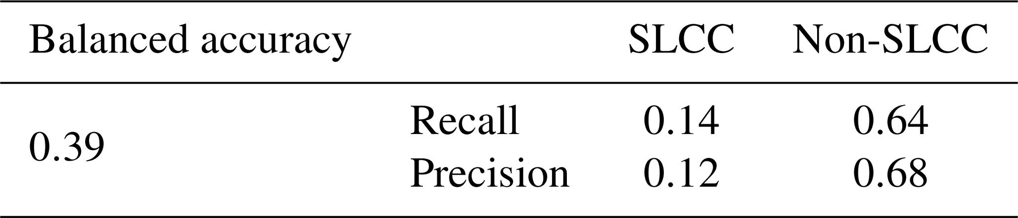
The XGBoost model was trained and tested with 3-fold stratified-group cross-validation, as discussed previously. Accuracy scores, as described in Sect. 2.4, are presented in Table 2 as the mean of the 3-fold training and testing scores, with the uncertainties derived from the standard deviation. We also applied G22-Davis to our dataset of peak properties and compared that model's binary prediction of SLCC to our reference mask's classification of each peak as SLCC. Accuracy scores for the G22-Davis model performance are presented in Table 3. These results demonstrate that the G22-Davis model performed poorly at SLCC classification in this environment relative to the excellent performance at Davis, where the model achieved accuracy scores as high as 0.91 (Guyot et al., 2022).

Table 2 G22-Christchurch model balanced accuracy scores as well as recall and precision scores for each class from 3-fold stratified-group cross-validation.

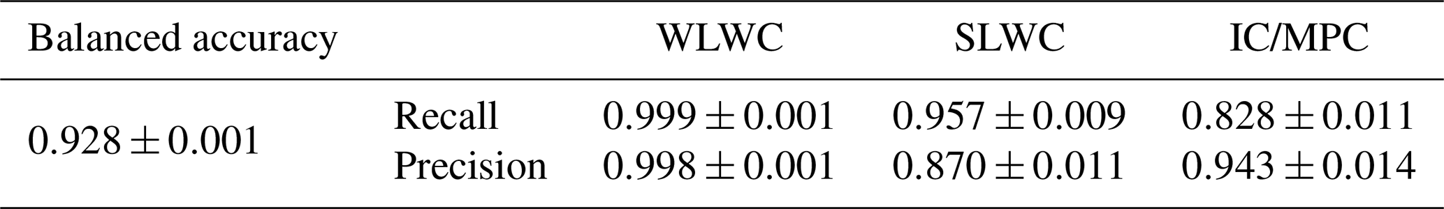
Table 3 G22-Davis model balanced accuracy scores as well as recall and precision scores for each class.

The performance of the G22-Christchurch cloud mask was then analysed by comparing the reference mask and the new model-generated SLWC mask, as described in Sect. 2.4. This involves the comparison of two one-dimensional Boolean vectors, corresponding to the reference mask and the model-generated mask. We first evaluate the performance of the model mask by comparing all profiles (time steps) and then compare only time steps where peaks meeting the minimum backscatter and width thresholds were detected. For the full dataset with 66 240 time steps, there were 31 708 time steps (47.9 %) where peaks were detected. This is lower than the total number of peaks (34 542) since some time steps contained multiple peaks corresponding to multilayer cloud. According to the reference mask, SLWC was present in 15.3 % of all profiles and 27.5 % of profiles with peaks. The recall (precision) of the G22-Christchurch SLWC mask was 0.76 (0.89) for all profiles and 0.88 (0.89) for profiles with peaks. The recall (precision) of the G22-Davis SLCC mask was 0.15 (0.15) for all profiles and 0.18 (0.15) for profiles with peaks. We repeated this analysis for WLWC detection by comparing the reference mask's WLWC label to our model's WLWC mask. According to the reference mask, WLWC was present in 45.1 % of all profiles and 67.2 % of profiles where peaks were detected. The recall (precision) of the G22-Christchurch WLWC mask was 0.63 (0.99) for all profiles and 0.88 (0.99) for profiles with peaks.

3.3 Case studies

In this section we present results showing the application of both our mask and the G22-Davis mask to two case studies in order to interpret their performance. Backscatter peaks from these days were excluded from the training dataset, so these days represent unseen data.

3.3.1 18 May 2021 case study

Observations from 18 May 2021 are shown in Fig. 5 as an example of a day with a distinct SLWC layer. Figure 5 shows the ALCF-calibrated attenuated volume backscatter (Fig. 5a), volume depolarization ratio (VDR) (Fig. 5b) and VDR reference cloud mask (Fig. 5c–d), along with the G22-Davis cloud mask (Fig. 5e–f) and G22-Christchurch cloud mask (Fig. 5g–h) applied to the attenuated backscatter profiles. The cloud masks are presented as time × altitude grids (Fig. 5c, e, g) and time step Booleans (Fig. 5d, f, h) according to whether SLWC is present anywhere in that profile. This particular day shows a clear band of SLWC between 06:00 and 12:00 UTC at 4 km altitude and again between 17:00 UTC on 18 May and 00:00 UTC on 19 May between 3–6 km. Other cloud (identified as IC and MPC by the VDR reference mask) is present from 02:30 to 06:00 UTC between 2–8 km altitude and again from 14:30 to 16:30 UTC. The first SLWC band is a multilayered cloud region between 06:00 and 08:00 UTC. Clouds or precipitation can be observed below the second SLWC band at around 20:00 and 22:00 UTC. According to the reference mask classification, a thin layer of WLWC below 1 km is also present from 19:00 UTC on 18 May to 00:00 UTC on 19 May. However, it is possible that this layer, which attenuates relatively little lidar signal as seen in Fig. 5a, could actually be an aerosol layer that has been misidentified as cloud by the ALCF cloud mask, as discussed in Sect. 2.2.

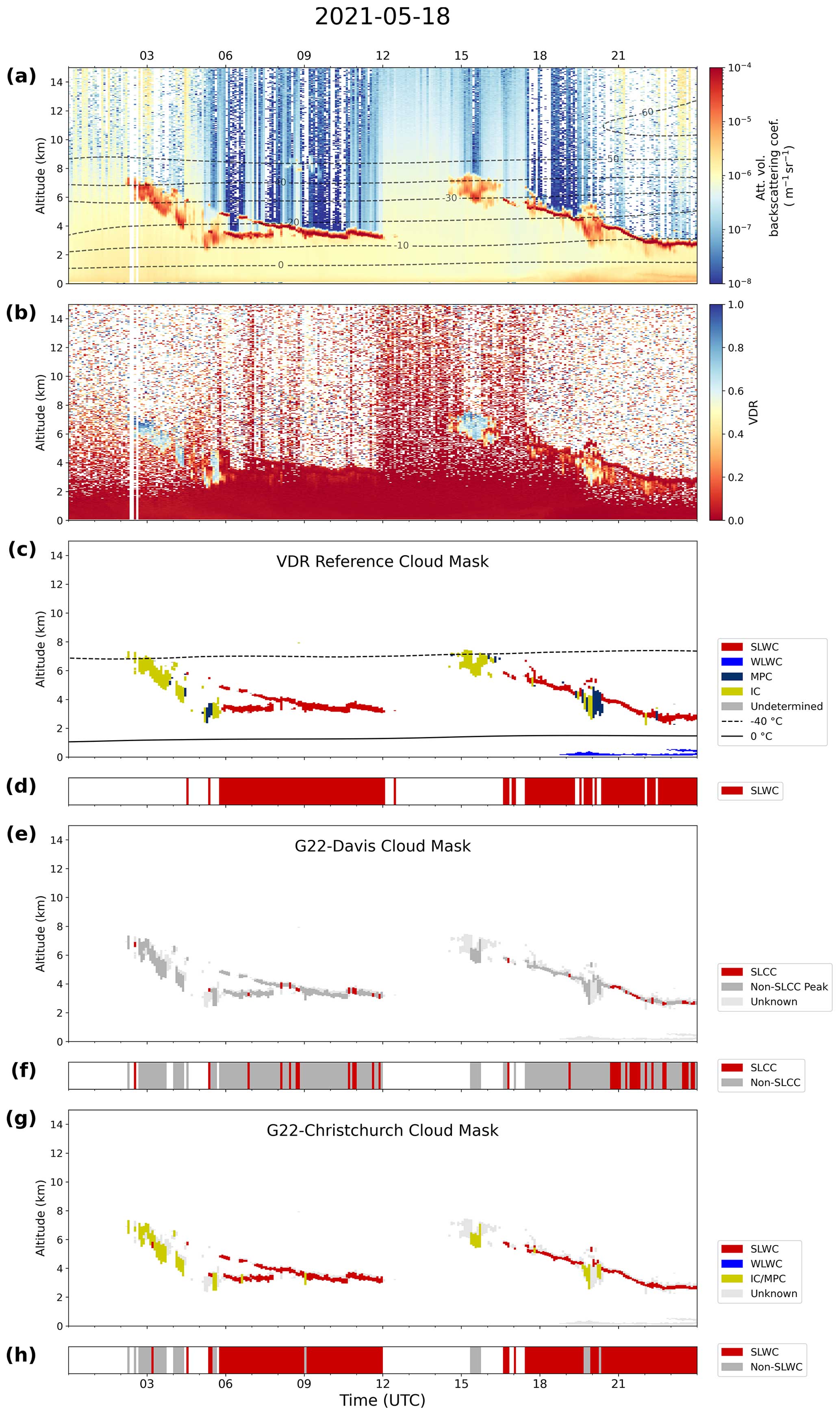
Figure 5 MPL profile for 18 May 2021 over Christchurch showing attenuated the volume backscatter coefficient (a), the volume depolarization ratio (VDR) (b), the VDR reference cloud mask (c), the G22-Davis cloud mask (e) and the G22-Christchurch cloud mask (g). Time step classifications of SLWCs are shown in (d, f, h) for the reference mask, G22-Davis and G22-Christchurch, respectively, along with time steps for which peaks were identified. WRF air temperature contours are overlaid in (a) and (c).

The G22-Davis cloud mask identifies some of the SLWC layers correctly but misses many. Comparing profile-to-profile SLCC classification to the reference mask, G22-Davis had recall (precision) scores of 0.19 (0.94) when considering all profiles and 0.20 (0.94) for profiles containing peaks. The new G22-Christchurch cloud mask performs better and identifies most of the SLWC layers. Compared to the reference mask's SLWC classification for each time step, G22-Christchurch had recall (precision) scores of 0.96 (0.94) for all profiles and 0.97 (0.94) for profiles containing peaks.

3.3.2 5 June 2021 case study

MPL observations from 5 June 2021 are shown in Fig. 6. On this day, a wide band of IC is present at altitudes ranging from 3–10 km between 00:00 and 18:00 UTC, followed by a band of low-altitude (< 1 km) liquid water cloud between 18:00 UTC on 5 June and 00:00 UTC on 6 June and another layer of liquid water cloud at around 2–3 km altitude for a short period after 22:00 UTC. Layers of SLWC are present for short periods throughout the day (06:00, 10:00, 12:00 and 14:00 UTC) interspersed with ice cloud (see Fig. 6c). Both G22-Davis and G22-Christchurch identify some of the short periods of SLWC between 06:00 and 15:00 UTC. G22-Christchurch correctly distinguishes most of the SLWC but also overestimates SLWC occurrence, making false positive classifications at around 07:00, 09:00 and 14:00 UTC. Importantly, the low-altitude WLWC band between 18:00 and 21:00 UTC is mistakenly identified as SLCC by G22-Davis. G22-Christchurch correctly identifies this layer as WLWC.

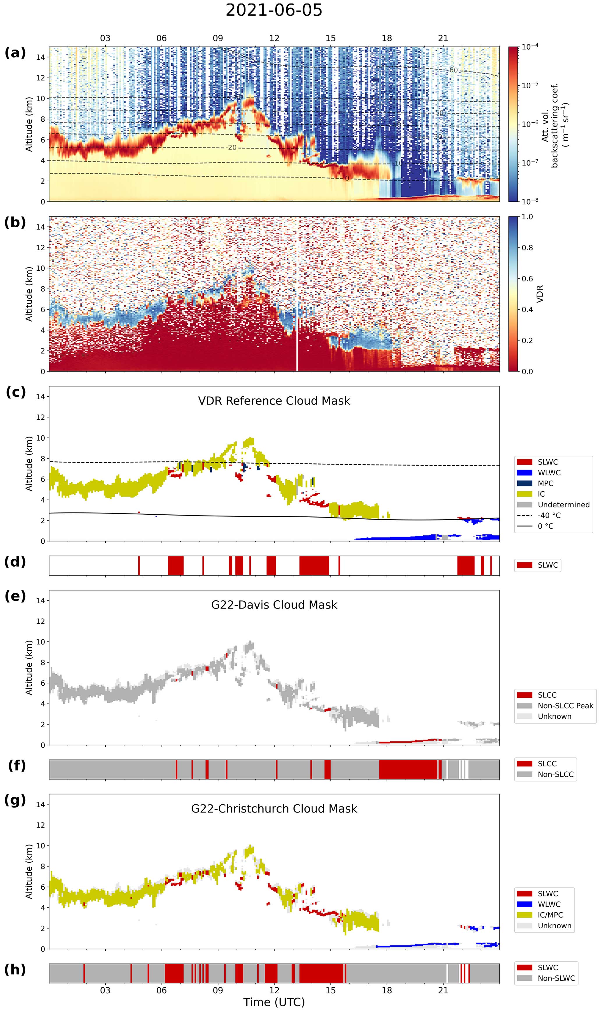
Figure 6 MPL profile for 5 June 2021 over Christchurch showing the attenuated volume backscatter coefficient (a), the volume depolarization ratio (VDR) (b), the VDR reference cloud mask (c), the G22-Davis cloud mask (e) and the G22-Christchurch cloud mask (g). Time step classifications of SLWC are shown in panels (d), (f) and (h) for the reference mask, G22-Davis and G22-Christchurch, respectively, along with time steps for which peaks were identified. WRF air temperature contours are overlaid in (a) and (c).

On this day, G22-Davis had recall (precision) scores of 0.09 (0.12) when compared to the reference mask's SLCC classification for all peaks and also 0.09 (0.12) when comparing profiles containing peaks. Again, the new G22-Christchurch performed much better, with recall (precision) scores of 0.75 (0.64) for all profiles and 0.80 (0.64) for profiles containing peaks, compared to the reference SLWC mask. These results show that the new model is a significant improvement to G22-Davis in environments that contain WLWC but still has limitations in identifying SLWC when interspersed with IC, which are conditions this case study represents. Despite this, these results indicate that the technique of Guyot et al. (2022) can be successfully applied to a new location if appropriate site-specific training data are available.

3.4 Cloud occurrence for the full observation period

The full dataset was analysed and cloud occurrence statistics computed to compare the accuracy of the G22-Davis and G22-Christchurch cloud masks to our VDR reference mask. In this section, we present cloud fraction statistics and cloud-phase distribution as a function of altitude for each mask and evaluate the performance of the G22-Christchurch cloud mask.

Cloud fraction was calculated by finding the proportion of profiles in which SLWC or WLWC was detected across all time steps of the dataset. The cloud fraction from all types (calculated from the ALCF cloud detection mask) was 70 % for the full dataset of 257 equivalent days of MPL profiles. SLWC was detected in 15.3 % of the reference mask profiles, 12.9 % of the G22-Christchurch mask profiles and 16.9 % of the G22-Davis mask profiles. Meanwhile, the WLWC frequency was 45.1 % for the reference mask but only 28.5 % for G22-Christchurch. G22-Davis overestimated the frequency of SLCC occurrence because it often misclassified WLWC layers as SLCC, such as between 18:00 and 21:00 UTC in Fig. 6. G22-Christchurch, however, tends to underestimate both SLWC and WLWC occurrence relative to the reference mask.

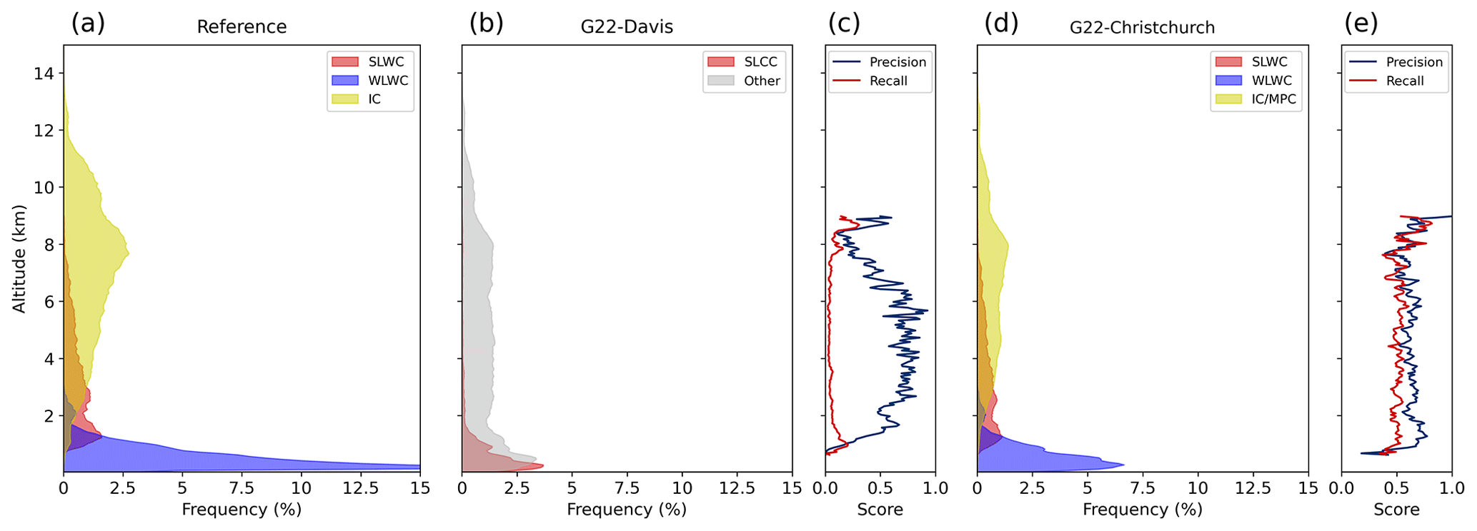
Figure 7 Cloud altitude distributions separated by cloud phase, according to the VDR reference mask (a), G22-Davis mask (b) and G22-Christchurch mask (d). Precision and recall accuracy scores for SLCC and SLWC detection, respectively, as a function of altitude, are also shown for G22-Davis (c) and G22-Christchurch (e).

Figure 7 compares the cloud-phase distributions as a function of altitude for G22-Davis and G22-Christchurch against the reference mask. According to the reference mask in Fig. 7a, liquid water cloud (WLWC and SLWC) is common at low altitudes and decreases in frequency with altitude to a maximum altitude of 8 km. Below 1 km, this is entirely WLWC, and above 3 km it is entirely SLWC, with the overlap between 1–3 km likely corresponding to the variation of the 0 °C isotherm through the year. This pattern is consistent with the peak altitude distributions shown in Figs. 3e and 4e. Ice cloud frequency increases with altitude to a maximum at 8 km, before decreasing to very low occurrences at 13 km.

Figure 7b shows that G22-Davis identifies SLCC at lower altitudes (0–4 km) than the reference mask (1–8 km). The recall and precision scores as a function of altitude, in Fig. 7c, are low for the G22-Davis model. This bias likely results from the Davis training dataset, which would indicate that SLCCs could be present at low altitudes despite the fact that temperatures at Davis for which SLCCs were detected were much lower. This therefore provides evidence of the limitation of applying the G22-Davis method, with training data from Davis, Antarctica, to mid-latitude sites with warmer air temperatures. This also shows the relative importance of peak altitude in the SLCC classification for G22-Davis.

Figure 7d shows cloud-phase distributions according to the G22-Christchurch cloud mask. The frequency of SLWC is highest at 1.5 km and gradually decreases with altitude until around 8 km, following a very similar pattern to the VDR reference mask's SLWC occurrence. WLWC occurrence also closely follows the reference mask's WLWC occurrence, with frequencies being highest at low altitudes and decreasing with altitude until around 2 km, but is still underestimated relative to the reference mask. In Fig. 7e, the precision and recall scores for SLWC detection as a function of altitude are relatively consistent, and recall scores are higher than the recall scores for G22-Davis in Fig. 7c at all altitudes.

Both G22-Davis and G22-Christchurch underestimate total cloud fraction across all cloud phases. One factor that may account for this is that the criteria for a peak to be selected for classification ($\mathit{\beta }>\mathrm{2}\times {\mathrm{10}}^{-\mathrm{5}}$) are stricter than the criteria for ALCF and the reference mask to detect a cloud ($\mathit{\beta }>\mathrm{4}\times {\mathrm{10}}^{-\mathrm{6}}$). We also found that the frequencies and accuracy scores in Fig. 7d and e were sensitive to the width of the generated cloud mask layer as defined by the upper and lower bounds around the peak location. Therefore, the cloud-phase distributions in Fig. 7 provide qualitative evidence of the model's performance, but quantitative results are best determined by comparing time step SLWC Booleans as in Sect. 3.2.

3.5 XGBoost feature analysis with SHAP

The previous sections have shown that our model performs very well at classifying backscatter peaks as SLWC or WLWC and reasonably well at generating cloud masks of SLWC and WLWC occurrence which are comparable to the reference VDR cloud mask. In order to be confident the model can be applied in future work to ceilometer datasets from a range of locations, we need to understand the relative importance of the input features to the XGBoost algorithm (our eight-feature set of peak properties).

Figure 8 shows correlation coefficients between each pair of peak properties for all peaks in the dataset. This allows for a visual analysis of the independence of the XGBoost input features. Figure 8 shows that peak magnitude, width height and prominence are strongly positively correlated, as we expect. Peak altitude and peak temperature are also strongly negatively correlated because low altitudes are associated with warmer temperatures, and high altitudes are associated with colder temperatures. We can also use Fig. 8 to select a subset of features that are independent by removing strongly correlated features. We use this information in Sect. 3.6 to train a modified model using a smaller range of independent input features.

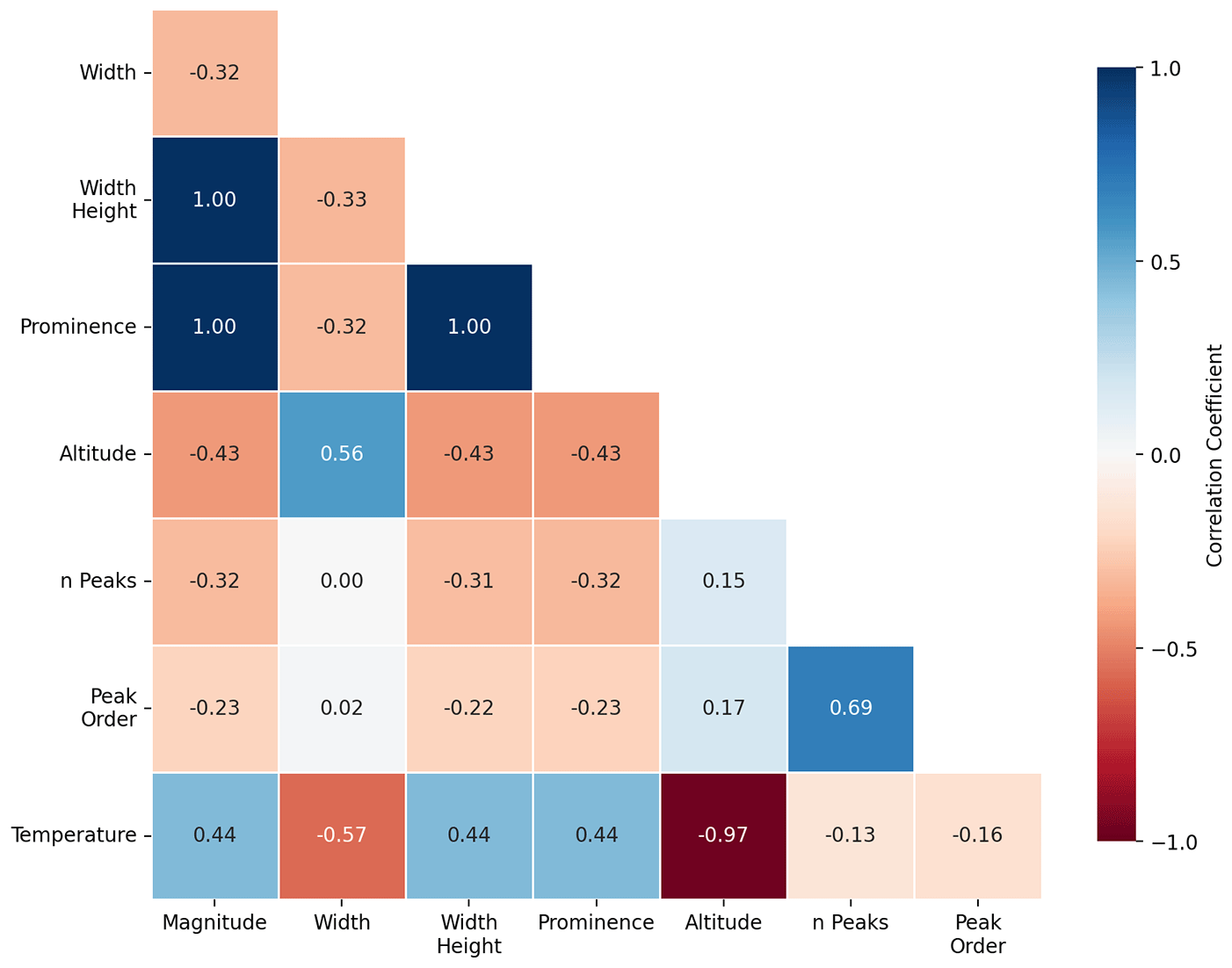
Figure 8 Correlation coefficients between each pair of peak properties for all peaks in the dataset.

Like Guyot et al. (2022), we apply the tree-based model explanation method by Lundberg et al. (2020) based on SHapley Additive exPlanations (SHAP) values, which quantify the contributions to the model output from each feature. Such an analysis is important for model interpretability, to ensure the model results are trustworthy, and to understand the relationships between the input features (in this case, the dataset of peak properties) and model output. Figure 9 shows the SHAP value distribution for the input features to G22-Christchurch. In this stacked bar plot, features are ranked from top to bottom according to their mean absolute SHAP value, i.e. from most to least important for the model's classification. The distribution of SHAP values for the three most important features (peak temperature, altitude and width) is further shown in Fig. 10, which shows SHAP value scatter plots corresponding to each feature for each class.

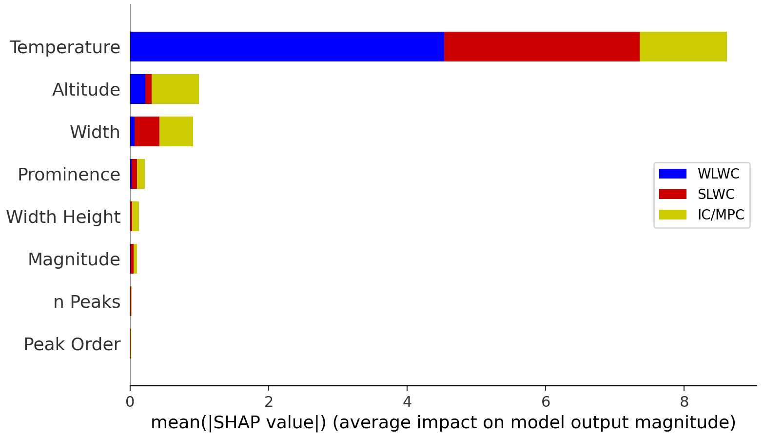
Figure 9 Mean absolute SHAP values for G22-Christchurch features for each class (SLWC, WLWC, and IC and MPC). Features are ranked from top to bottom according to the sum of the mean absolute SHAP value across all classes, i.e. most to least important for the overall classification.

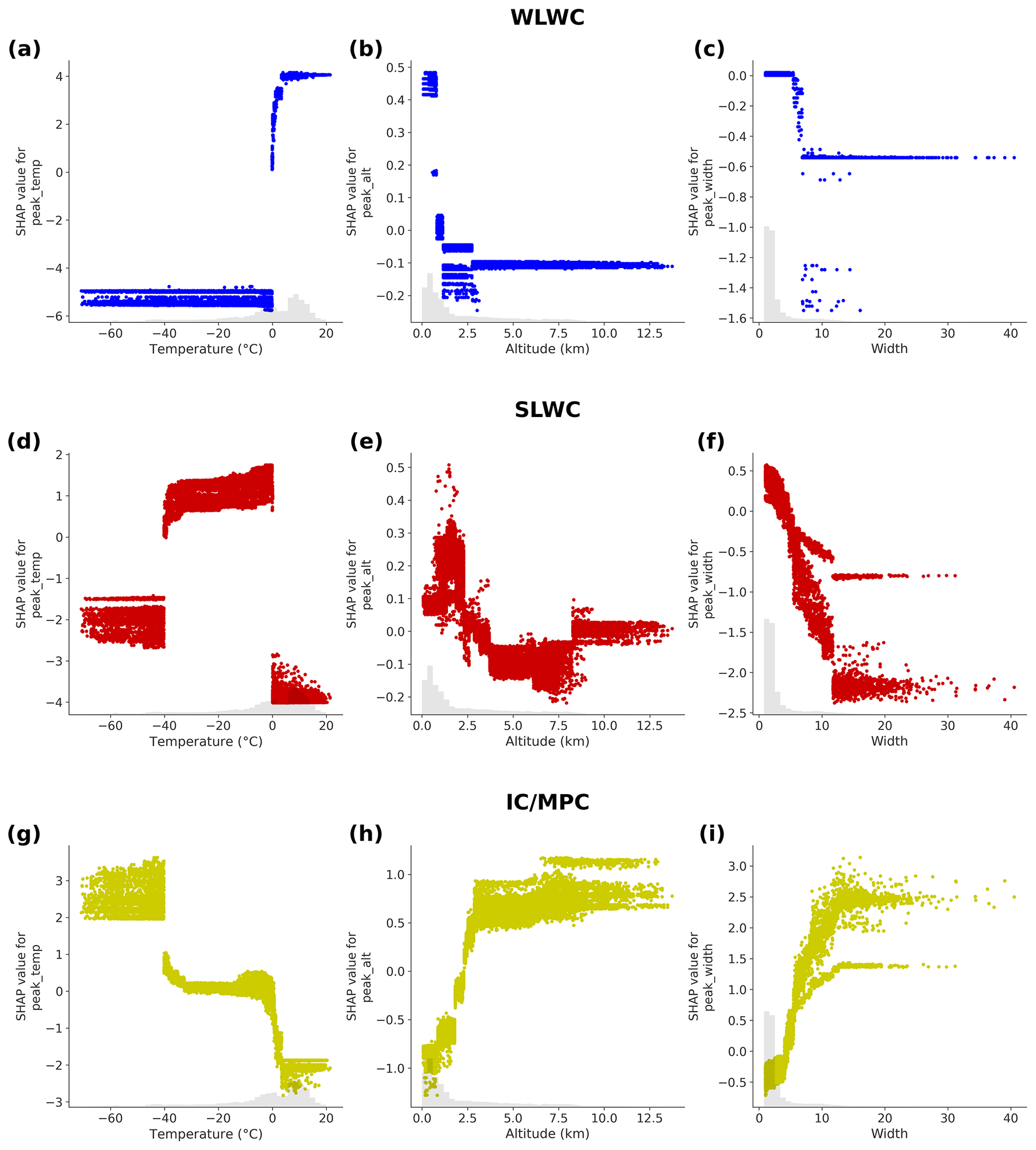
Figure 10 SHAP value scatter plots for peak temperature, altitude and width for WLWC (a–c), SLWC (d–f), and IC and MPC (g–i).

Temperature is shown in Fig. 9 to be the most important feature for classification across all classes, and the relationships shown in Fig. 10a, d and g reveal how XGBoost uses temperature to improve classifications. Figure 10d shows that SHAP values for SLWC classification are positive for temperatures between −40 and 0 °C and negative outside this range. On the other hand, the SHAP values for WLWC classification are positive above 0 and negative below 0 °C. The strong discontinuity at 0 °C for classification of both SLWC and WLWC occurs because the VDR reference mask uses that temperature for distinguishing between SLWC and WLWC. Figure 10g shows that the opposite is true for IC and MPC classification: SHAP values are strongly positive below around −40 °C (since only ice is found at these temperatures), are strongly negative above 0 °C and have intermediate values in the mixed-phase temperature regime.

Altitude and temperature are inversely correlated (as shown in Fig. 8) because low altitudes are associated with warmer temperatures, and high altitudes are associated with colder temperatures. Figure 9 shows peak altitude to be the second-most useful feature after temperature, with mean absolute SHAP values roughly equal across all classes. Figure 10h shows that higher values of altitude were more strongly associated with IC and that low altitudes had a negative impact on IC classification. Figure 10b shows that for WLWC, low values of altitude have positive SHAP values and a positive impact on WLWC classification. As altitude increases, SHAP values become more negative, meaning these values have a negative impact on WLWC classification, as supported by the fact that Fig. 7a shows very little WLWC occurrence above 3 km. The SHAP value distribution for SLWC classification (Fig. 10e) is more complex but generally shows that as altitude increases, SHAP values tend to decrease, as supported by Fig. 7a showing a decreasing frequency of SLWC up to around 8 km. In Fig. 10e, for altitudes above 8 km, SHAP values tend to zero, showing that these values have neither a positive nor a negative impact on SLWC classification.

Next, Fig. 9 shows peak width to be a highly useful feature. The SHAP value scatter plots shown in Fig. 10f and i show the relationship between peak width and SLWC or IC classification. Figure 10f shows that low values of peak width had a positive impact on SLWC classification and that high values had a negative impact. This agrees with our physical understanding of the properties of backscatter from liquid water cloud as discussed previously, namely that liquid water rapidly attenuates the lidar signal, leading to a narrow band of enhanced returned backscatter. The reverse is true for IC and MPC classification, shown in Fig. 10i, where a low value of peak width is associated with a negative IC classification, and higher values of peak width had a positive impact on IC classification.

While Fig. 3 shows that there was a slight separation in the distribution of liquid and non-liquid peak backscatter magnitudes, the SHAP values in Fig. 9 show that peak magnitude was not a highly useful feature for the G22-Christchurch model in any class. Peak prominence, which we show in Fig. 8 to be strongly positively correlated with peak magnitude, has a higher mean absolute SHAP value, indicating it is more useful than magnitude for classification. Scatter plots of SHAP values found that low prominence peaks had a positive impact on IC classification, and high prominence peaks had a positive impact for SLWC and WLWC classification (not shown). One possibility for why magnitude is less useful than prominence is that magnitude is already the main criterion used to select peaks. That is, we only analyse peaks that already exceed a backscatter threshold of $\mathit{\beta }>\mathrm{2}\times {\mathrm{10}}^{-\mathrm{5}}{\mathrm{m}}^{-\mathrm{1}}{\mathrm{sr}}^{-\mathrm{1}}$, which excludes most low-β peaks associated with IC. Peak prominence, however, provides a way of separating peaks with a higher signal-to-noise ratio (SNR) and is therefore more useful than peak magnitude. The results here differ from the results found by Guyot et al. (2022). In that study, peak magnitude was found to be the most significant feature used by XGBoost for the classification of SLCC. However, the aim of the G22-Davis model was to distinguish SLCC and ice, while our aim is to distinguish SLWC, WLWC and IC. Therefore, it is logical that our highest-scoring features are temperature and altitude, which are powerful at distinguishing SLWC and WLWC (as shown in Fig. 4), whereas the Guyot et al. (2022) highest-scoring feature was peak magnitude, which was powerful at distinguishing SLCC and ice. Therefore, the SHAP value differences between G22-Davis and G22-Christchurch are likely a consequence of the different classification objectives of the two models.

3.6 Reducing XGBoost feature dimensionality

Due to the strong correlation between input features, as shown in Fig. 8, we next investigate the effect of reducing the number of input features to train a modified XGB model. Reducing the dimensionality of the training dataset has been shown to improve model performance in general by reducing overfitting (Russell and Norvig, 2010). Furthermore, excluding temperature would remove the dependence on numerical weather prediction model inputs which clearly include uncertainty. We trained a new set of XGBoost models using a reduced set of input features, testing various combinations of those input features with the highest mean absolute SHAP values, as detailed in Fig. 9, and removing “duplicate” features that are strongly correlated, as determined in Fig. 8. For example, because peak magnitude, prominence and width height are strongly correlated, we only use one of those features as input to a model. The same is true for peak altitude and temperature, which are strongly negatively correlated. We also remove the number of peaks and peak order because they have low absolute SHAP values, as shown in Fig. 9. These results are presented in Table 4, which shows the various input features and accuracy scores of the corresponding XGBoost models, again tested with 3-fold stratified-group cross-validation in each case. The same set of hyperparameters was used during the development of these models to allow a direct comparison with the original eight-feature model. The entire dataset of peak properties was used for the development of these models, hence the difference from the scores presented in Table 2.

Table 4 Summary of the balanced accuracy scores as well as precision and recall scores for each class from 3-fold stratified-group cross-validation for the adjusted models with reduced input features: peak temperature T, peak altitude z, peak width w, peak magnitude β, peak prominence β_prom and peak width height β_w.

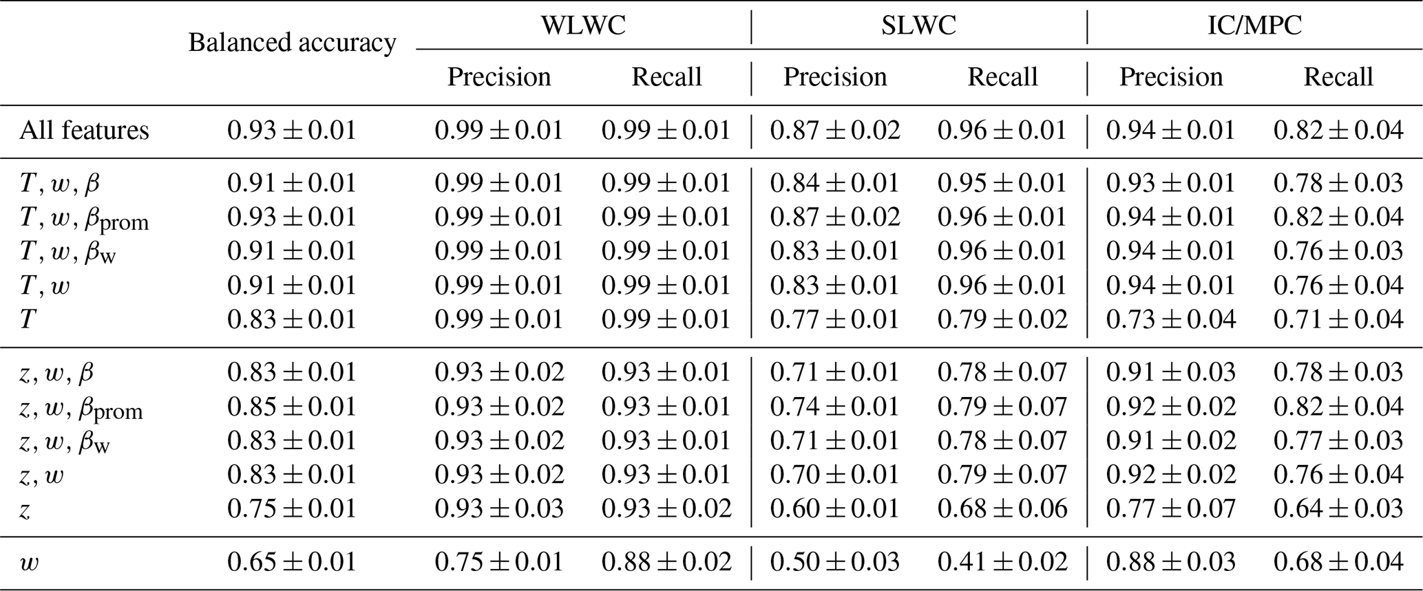
We see from Table 4 that the highest-scoring model used the input features temperature, peak width and peak prominence ($T,w,{\mathit{\beta }}_{\mathrm{prom}}$), and it performed equally well as the original model that used the complete set of eight features. This is consistent with the results in Sect. 3.5, where we show using SHAP values that these were among the most useful features for G22-Christchurch. Replacing peak prominence with either peak magnitude or peak width height slightly reduced the accuracy, and removing it entirely (without replacement) also only slightly reduced the accuracy. The model using just peak temperature as an input still gave reasonable accuracy scores, although the drop of 0.17 in the SLWC recall score from the (T,w) model shows the importance of peak width as an input feature. However, it is worth noting that peak width and magnitude are both essential features for identifying clouds and therefore peaks in the first place. Replacing peak temperature with peak altitude reduced the balanced accuracy by around 0.08 for all models, and reduced the recall scores by around 0.17 for SLWC and 0.07 for WLWC across all models. This significant reduction in model performance shows that despite peak altitude and peak temperature being strongly negatively correlated, altitude was not a useful direct replacement for temperature. This confirms the importance of having either NWP temperature information or radiosonde temperature data for making accurate classifications of SLWC. However, recall scores for WLWC were still high (> 0.9) and generally unchanged for IC and MPC (around 0.8) when temperature was replaced with altitude, indicating that liquid–ice classification can generally be made without temperature information (i.e. without distinguishing SLWC and WLWC).

4 Conclusions

In this study, we applied a method of supercooled liquid water cloud (SLWC) detection first introduced by Guyot et al. (2022) to observations from a mid-latitude site. From a 9-month dataset of micro-pulse lidar (MPL) co-polarized backscatter peak properties, we then trained an optimized gradient boosting model to classify backscatter peaks as SLWC, warm liquid water cloud (WLWC), or ice- and mixed-phase cloud (IC and MPC). Unlike the binary supercooled-liquid-water-containing cloud (SLCC) classification model developed by Guyot et al. (2022), referred to as G22-Davis to reflect the fact that the training dataset was from Davis Station, Antarctica, our model performed multi-class classification to distinguish SLWC from WLWC, which was common in our lidar observations from Christchurch, New Zealand.

We first used MPL depolarization observations to build a reference cloud-phase mask which uses the volume depolarization ratio (VDR) to distinguish ice and liquid; we then used WRF-derived air temperatures to distinguish SLWC and WLWC. Applying G22-Davis to our dataset of co-polarized backscatter peak properties to create an SLCC classification mask, we obtained recall scores of 0.15 when examining all lidar profiles and 0.18 when examining only profiles with detection of strong backscatter signals. We then trained and tested a modified XGBoost model, referred to as G22-Christchurch, and applied it to the same MPL dataset to create an SLWC mask with recall scores of 0.76 for all profiles and 0.88 for profiles with strong backscatter signals. G22-Christchurch greatly improved classification of SLWC compared to G22-Davis, which often misclassified WLWC as SLCC due to the absence of warm liquid water in the Davis training data.

We also applied the tree-based model explanation method by Lundberg et al. (2020) based on SHapley Additive exPlanations (SHAP) values to quantify the relative importance of each XGBoost input feature (Lundberg and Lee, 2017). We found that temperature was the most important feature for SLWC and WLWC classification due to the homogeneous freezing of liquid water at around −40 °C and the definition that SLWC exists below 0 °C. Peak width was the most important peak property for detecting liquid water of either type because liquid water rapidly attenuates the lidar signal, causing a narrow peak in the returned backscatter profile. Peak prominence was also a useful feature for SLWC classification. We then developed a set of models with reduced input features and compared their accuracies with the original model. We found that using only peak temperature, width and prominence as inputs, an XGBoost model could perform equally well as the original model trained using the full set of peak properties. Despite being strongly negatively correlated with temperature, peak altitude was not a suitable replacement for temperature for SLWC classification. This confirms the importance of air temperature data availability, such as from NWP models, for accurate detection of SLWC alongside ceilometer observations. This differs from the findings of Guyot et al. (2022); however, it is important to note that our objectives differ. In this study, features that distinguish SLWC and WLWC are highlighted (i.e. temperature), whereas for Guyot et al. (2022), the best features that distinguished SLWC and ice were identified (i.e. peak magnitude). When using our model to distinguish ice from liquid (of either WLWC or SLWC), the set of peak properties without temperature still gave good results, showing that liquid classification can be performed without relying on other sources for temperature information. For future work, such as the incorporation of this retrieval method in ALCF, the default XGBoost model will only use peak width, prominence and temperature as inputs, while a model using width, prominence and altitude as inputs will be an alternative for cases when temperature data are unavailable.

The frequency of SLWC occurrence was analysed for G22-Davis and G22-Christchurch and compared to our reference mask. Cloud fraction according to the reference mask was 15 % for SLWC and 45 % for WLWC. WLWC was only present at low altitudes, below 2 km, and SLWC was present between 1–8 km. G22-Davis often misclassified WLWC as SLWC, which caused that model to incorrectly inflate SLWC occurrence below 2 km. On the other hand, G22-Christchurch replicated the reference mask's vertical structure of SLWC and WLWC occurrence, although cloud occurrence was still generally underestimated across all phase categories.

The limitations of the relatively simple VDR reference mask should be noted. In some cases, high aerosol loads near the ground were falsely classified as WLWC by the reference mask. Precipitation and fog were not represented by the reference mask and may have been misidentified as IC, MPC or WLWC. Previous methods (Tuononen et al., 2019; Guyot et al., 2022) have classified precipitation and fog using attenuated backscatter thresholds and gradients, which was not performed in this study. This may have artificially inflated the attenuated backscatter coefficient and therefore peak magnitudes in WLWC and IC clouds. The effects of multiple scattering may also have caused some liquid layers to be misclassified as IC. On the other hand, horizontally aligned ice crystals may have caused some ice cloud to be misidentified as liquid, since the MPL was oriented toward the zenith. This effect may have also caused ice particles to return higher than normal co-polarized attenuated backscatter (Hogan and Illingworth, 2003), potentially influencing the distribution of IC peak properties and therefore the usefulness of peak magnitude for G22-Christchurch in distinguishing liquid and ice. The reference mask classification of SLWC and WLWC relies on WRF-derived temperature data, which have their own associated uncertainty. In future work, more focus should be given to quantifying that error, such as using in situ (e.g. radiosondes) or remote measurements of cloud temperature. Additionally, it should be noted that the minimum detection height of the MPL is 100 m. Therefore, the MPL analysis in this work potentially misses low-level cloud, which Griesche et al. (2024) identified as an important polar cloud regime for future observational studies.

The aim of this study was to understand the limitations of G22-Davis at a mid-latitude site where both supercooled liquid and warm liquid water clouds exist. Ceilometers, being relatively common and low-cost, have the potential to be a useful tool for the detection of SLWCs and have particular value in regions where observations are sparse, such as Antarctica and the Southern Ocean. Ground-based ceilometer observations, complementary to satellite observations, have the potential to improve cloud-phase products. We found that while the methodology of G22-Davis was successful when used with a local training dataset, the original Davis-trained model was not effective at classifying SLWC over Christchurch. This confirms the need for further testing in different regions under different environmental conditions. The G22-Christchurch model and algorithm will be incorporated in future versions of ALCF so that future work can apply this retrieval technique to other lidar and ceilometer datasets.