the Creative Commons Attribution 4.0 License.
the Creative Commons Attribution 4.0 License.
NitroNet – a machine learning model for the prediction of tropospheric NO2 profiles from TROPOMI observations
Steffen Beirle
Sergey Osipov
Andrea Pozzer
Thomas Wagner
We introduce NitroNet, a deep learning model for the prediction of tropospheric NO2 profiles from satellite column measurements. NitroNet is a neural network trained on synthetic NO2 profiles from the regional chemistry and transport model WRF-Chem, which was operated on a European domain for the month of May 2019. This WRF-Chem simulation was constrained by in situ and satellite measurements, which were used to optimize important simulation parameters (e.g. the boundary layer scheme). The NitroNet model receives NO2 vertical column densities (VCDs) from the TROPOspheric Monitoring Instrument (TROPOMI) and ancillary variables (meteorology, emissions, etc.) as input, from which it reproduces NO2 concentration profiles. Training of the neural network is conducted on a filtered dataset, meaning that NO2 profiles showing strong disagreement (>20 %) with colocated TROPOMI column measurements are discarded.
We present a first evaluation of NitroNet over a variety of geographical and temporal domains (Europe, the US West Coast, India, and China) and different seasons. For this purpose, we validate the NO2 profiles predicted by NitroNet against satellite, in situ, and MAX-DOAS (Multi-Axis Differential Optical Absorption Spectroscopy) measurements. The training data were previously validated against the same datasets. During summertime, NitroNet shows small biases and strong correlations with all three datasets: a bias of +6.7 % and R=0.95 for TROPOMI NO2 VCDs, a bias of −10.5 % and R=0.75 for AirBase surface concentrations, and a bias of −34.3 % to +99.6 % with R=0.83–0.99 for MAX-DOAS measurements. In comparison to TROPOMI satellite data, NitroNet even shows significantly lower errors and stronger correlation than a direct comparison with WRF-Chem numerical results. During wintertime considerable low biases arise because the summertime/late-spring training data are not fully representative of all atmospheric wintertime characteristics (e.g. longer NO2 lifetimes). Nonetheless, the wintertime performance of NitroNet is surprisingly good and comparable to that of classic regional chemistry and transport models. NitroNet can demonstrably be used outside the geographic and temporal domain of the training data with only slight performance reductions. What makes NitroNet unique when compared to similar existing deep learning models is the inclusion of synthetic model data, which offers important benefits: due to the lack of NO2 profile measurements, models trained on empirical datasets are limited to the prediction of surface concentrations learned from in situ measurements. NitroNet, however, can predict full tropospheric NO2 profiles. Furthermore, in situ measurements of NO2 are known to suffer from biases, often larger than +20 %, due to cross-sensitivities to photooxidants, which other models trained on empirical data inevitably reproduce.
- Article
(16500 KB) - Full-text XML
- BibTeX
- EndNote
Nitrogen oxides (NOx= NO + NO2) are an important marker of air pollution. The negative impact of NO2 on human health has been widely recognized (see e.g. Faustini et al., 2014; Mills et al., 2015; Chowdhury et al., 2021). In many European countries, the recommended annual average exposure limit of 10 µg m−3 (see World Health Organization, 2021) is exceeded continuously. Active monitoring of tropospheric NO2 is a crucial step in identifying pollution hotspots, localizing emissions, and designing long-term solutions to the pollution problem. Different measuring methods for NO2 exist. Many countries across the world deploy in situ measurements at the surface (see e.g. the AirBase network; European Environment Agency, 2024). The TROPOspheric Monitoring Instrument (TROPOMI; see Veefkind et al., 2012) yields measurements of tropospheric NO2 vertical column densities (VCDs), with daily near-global coverage and a ground pixel size of up to 3.5 km×5.5 km. Lastly, ground-based MAX-DOAS (Multi-Axis Differential Optical Absorption Spectroscopy) measurements (see Platt and Stutz, 2008; Hönninger et al., 2004) are used to obtain tropospheric NO2 profiles in a few selected places by means of scanning the troposphere at different elevation angles. Although further measuring platforms (e.g. sondes and aircraft) and methods (e.g. light detection and ranging (lidar) instruments or cloud slicing) exist, these are not routinely deployed (see e.g. Sluis et al., 2010; Bourgeois et al., 2022; Lange et al., 2023; Riess et al., 2023; Volten et al., 2009; Berkhout et al., 2018; Su et al., 2021; Marais et al., 2021). Particularly, aircraft measurements and cloud slicing are appreciated for their ability to resolve along the vertical axis, albeit at lower spatio-temporal resolutions (e.g. cloud slicing exhibits seasonal means with a 1° × 1° horizontal resolution and five tropospheric layers; see Marais et al., 2021) or with sparse spatio-temporal coverage (aircraft measurements). Altogether, these measurements are valuable for the quantification of tropospheric vertical column densities, surface concentrations, and to some extent tropospheric profile shapes. Nonetheless, the described methods also have the following drawbacks:
-
TROPOMI can measure the tropospheric column density, but it cannot resolve along the light path or the vertical axis, meaning it cannot principally return vertical NO2 profiles. Furthermore, the TROPOMI NO2 VCD retrieval depends on a priori profiles. In the operational TROPOMI processor, these profiles are taken from the TM5-MP model (see Krol et al., 2005), whose low horizontal resolution of 1° × 1° is known to be one of the main causes of significant negative biases, typically between −10 % and −20 % (see Ialongo et al., 2020; Tack et al., 2021; Liu et al., 2021; Douros et al., 2023) and in some cases even up to −50 % (Lange et al., 2023). Alternative data products with higher-resolution a priori profiles exist but are not available globally.
-
In situ measurements often utilize the molybdenum-based chemiluminescence method, which is known for its severe cross-sensitivities to other atmospheric oxidants, causing large biases in the reported NO2 concentrations (see Dunlea et al., 2007; Steinbacher et al., 2007; Lamsal et al., 2008; Boersma et al., 2009; Villena et al., 2012). These biases typically range from +20 % to +100 %, but Villena et al. (2012) report biases of up to +300 % in extreme cases. As described in detail later in the article, these biases can be strongly reduced to a few percent within our model framework.
-
MAX-DOAS measurements are quite sparsely located and cannot provide dense spatial coverage. Additionally, the commonly used retrieval algorithms suffer from significantly reduced sensitivity at higher altitudes (>2 km) and depend on a priori assumptions. An intercomparison study of MAX-DOAS retrieval algorithms by Tirpitz et al. (2021) revealed relative retrieval uncertainties of between 3 % and 70 %, which can be expected to be the dominant part of the total MAX-DOAS uncertainty.
Measurements are therefore often complemented by regional chemistry and transport (RCT) simulations. Examples of state-of-the-art RCT models include WRF-Chem (Grell et al., 2005), COSMO/MESSy (Kerkweg and Jöckel, 2012), LOTOS-EUROS (Manders et al., 2017), CAM-chem (Emmons et al., 2020), and CHIMERE (Menut et al., 2021). Such models can simulate realistic distributions of NO2 and other atmospheric trace gases with horizontal resolutions on the scale of 3 km×3 km and vertical resolutions of ∼1 m at the surface to ∼1 km in the upper troposphere. High-resolution RCT simulations can be used to estimate air pollution in the absence of in situ measurements and to obtain better-resolved a priori profiles for the TROPOMI retrieval. Unfortunately, the continuous deployment of RCT simulations is no easy endeavour due to their computational expense; their dependence on input data, which may not always be available in an up-to-date form at a high resolution (particularly the case for emission data); and the uncertainty in the choice of simulation parametrizations. Another point of concern is the general accuracy of these models. RCT simulations reported in recent literature have shown significant deviations from observational reference data (see Visser et al., 2019; Kuik et al., 2016, 2018; Poraicu et al., 2023), e.g. an underestimation of summertime surface-level NO2 concentrations of up to −50 %. A study by Douros et al. (2023) reveals overestimations of the wintertime NO2 VCD by +50 % and demonstrates that such biases even occur in ensemble models, such as the Copernicus Atmosphere Monitoring Service (CAMS) model (consisting of 11 different RCT models with a 0.1° × 0.1° horizontal resolution). In previous work, we showed that a recalibration of the vertical mixing parametrization can mostly resolve such biases in the WRF-Chem model during summer over Europe (see Kuhn et al., 2024). However, the process of model recalibration is tedious, computationally expensive, and domain-dependent. Altogether, it can be concluded that high-resolution RCT simulations are of undisputed benefit, but their practical realization remains challenging.
In this article, we introduce NitroNet, a new machine learning model intended to complement existing RCT models and measurements of NO2. NitroNet is a feed-forward neural network designed to predict full tropospheric NO2 profiles using TROPOMI VCDs alongside other ancillary data (meteorology, emissions, surface types, etc.) as input. Because neural networks are universal function approximators, they are the ideal tool for capturing such complex data relationships. NitroNet is trained on numerically simulated data from the WRF-Chem model, operated on a European domain for the month of May 2019, as described in Kuhn et al. (2024). A data-filtering scheme is used to ensure that only well-validated results from the WRF-Chem simulation are used to train the neural network (e.g. training examples with significant disagreement with colocated satellite observations are dismissed). Afterwards, NitroNet is used as a standalone model, without the need to run the RCT simulation again. By including synthetic model data, NitroNet expands on previous deep learning models trained on empirical data (see e.g. Gardner and Dorling, 1999; Kang et al., 2021; Chan et al., 2021; Ghahremanloo et al., 2021; Zhang et al., 2022; Jesemann et al., 2022; Cao, 2023; all presented models were trained on in situ surface observations). This approach provides intrinsic advantages. Firstly, NitroNet can predict full NO2 profiles, while models trained on empirical data can only be used for surface predictions. Secondly, the chemical mechanisms of RCT models allow for the explicit treatment of in situ measurement biases (typically larger than +20 %) by computing suitable correction factors, while empirically trained models cannot compute such correction factors and inevitably reproduce the biases inherent in the training data. Thirdly, synthetic datasets of NO2 profiles are typically much larger than the limited empirical data, and they also cover the spatial domain continuously. This allows for the use of highly selective training data filtering, which demonstrably improves the neural network's performance.
The article is structured as follows. Section 2 gives an overview of the datasets used in our study. Section 3 gives a detailed explanation of the NitroNet model. Section 4 presents an evaluation of NitroNet against satellite, in situ, and MAX-DOAS data on a European domain for May 2022 (i.e. on input data that the neural network has never seen before). This study is then extended to different seasons and geographical domains (UK, Spain and Portugal, the US West Coast, India, and China). Section 5 concludes the article.
The following datasets are used in our study:
2.1 Vertical NO2 profiles from WRF-Chem
An RCT simulation using the WRF-Chem model (version 4.2.2; see Grell et al., 2005) provides the NO2 profiles on which NitroNet is trained. The simulation was run for the month of May 2019 on a domain over Europe with a spatial resolution of 3 km×3 km, 43 terrain-following pressure levels, and hourly output. A detailed description, discussion, and validation study of this dataset were published in Kuhn et al. (2024). This study revolved around the question of how certain WRF-Chem model parameters can be optimized in order to improve the model's agreement with various reference datasets. In particular, optimization of the model’s vertical mixing parametrization was found to be crucial to improving the agreement with in situ observations of surface NO2. Unfortunately, such optimization problems take a long time to solve if the underlying model is as computationally expensive as WRF-Chem. Additionally, wintertime RCT simulations are known to be particularly challenging (see e.g. Douros et al., 2023), mainly due to their tendency to severely overestimate the total NO2 columns. Therefore, full-year training data with a resolution and accuracy comparable to our summertime data cannot be provided for now. Although NitroNet was trained exclusively on summertime data, it can be used in other seasons as well, albeit with larger prediction errors (as discussed in Sect. 4.3).
The simulation setup additionally deploys the vertical emission profiles from Bieser et al. (2011). We will refer to this dataset as “WRF-2019” from hereon. WRF-2019 contains approximately 2 million NO2 profiles, which are split into three partitions: a training set (80 %), a validation set (15 %), and a test set (5 %). The training set is used to train NitroNet (described in Sect. 3.3), the validation set is used for hyperparameter optimization (described in Sect. 3.2 and Appendix A), and the test set is used to evaluate the neural network on previously unseen data. The partitioning is obtained using unweighted random sampling without replacement.
2.2 Input data for NitroNet
NitroNet uses tropospheric NO2 vertical column densities (VCDs) from TROPOMI as the main input. Additionally, although much less influential, total O3 VCDs are used, assuming they are informative of the tropospheric O3 column and, thus, of tropospheric NOx photochemistry. The TROPOMI device on board the Sentinel-5P (S5P) satellite observes spectra of backscattered light from space with near-global coverage, a daily overpass at around 13:30 local time, and a pixel size of up to 3.5×5.5 km (see Veefkind et al., 2012; van Geffen et al., 2022). The retrieval of tropospheric NO2 VCDs is comprised of three steps. First, the NO2 total slant column density (SCD) is obtained from the observed light spectra using differential optical absorption spectroscopy (DOAS; see Platt and Stutz, 2008). Then, the obtained total SCD is separated into a stratospheric component and a tropospheric component (SCDtrop). Finally, the tropospheric VCD is obtained by computing
where AMFtrop denotes the tropospheric air mass factor. Air mass factors (AMFs) are computed using an altitude-dependent lookup table together with simulated NO2 a priori profiles from the RCT model TM5-MP (see Krol et al., 2005), with a horizontal resolution of 1° × 1°. The process is described by van Geffen et al. (2022). Throughout our study, we only use data with a high quality assurance value (fQA>0.75), which is the general recommendation (see Eskes et al., 2019). This high value also acts as a cloud filter as it removes observations with cloud fractions above 50 %. Throughout the rest of the paper, NO2 VCD refers to the tropospheric NO2 VCD, and O3 VCD refers to the total O3 VCD.
Additionally, NitroNet uses meteorological variables from the ERA5 reanalysis (0.25° × 0.25°; see Hersbach et al., 2020) and emission data from the EDGARv5 global emission inventory (0.1° × 0.1°; see Crippa et al., 2020) as input data.
2.3 Validation data for NitroNet
The following three datasets are used to evaluate the NitroNet model:
-
The aforementioned tropospheric NO2 VCDs from TROPOMI are used.
-
In situ surface measurements of NO2 from the European AirBase instrument network (see European Environment Agency, 2024) are employed. This dataset is assembled from the submissions of individual countries in the European Union. The measurements are available as hourly mean values and are classified into three groups: background, traffic, and industrial measurements. Traffic and industrial stations are typically located directly next to strong sources (e.g. near large streets or power plants), where strong horizontal NO2 gradients occur on the scale of a few metres (see e.g. Beckwith et al., 2019). Such gradients can be resolved neither by TROPOMI, whose observations are used as input data, nor by WRF-Chem, whose simulation results were used to train NitroNet. Therefore, only background stations are included in our validation study.
-
NO2 concentration profiles from MAX-DOAS instruments, operated within the FRM4DOAS (Fiducial Reference Measurements for Ground-Based DOAS Air-Quality Observations) project in Europe (see Fayt et al., 2021), are also used. FRM4DOAS uses the optimal-estimation-based Mexican MAX-DOAS fit (MMF; see Friedrich et al., 2019) and the Mainz profile algorithm (MAPA; see Beirle et al., 2019) for profile inversion. The resulting NO2 profiles are defined on a vertical grid with approximately ∼200 m spacing, reaching altitudes of up to 4 km. Each instrument produces approximately five NO2 profiles per hour. All profiles flagged as “erroneous” by MAPA were discarded. Note that although MAPA does not support automatic cloud filtering yet, the described error flagging has been shown to be sensitive to cloud effects as well (see Beirle et al., 2019).
The NitroNet model consists of an artificial neural network at its core and deploys additional non-machine learning code for efficient data pre-processing and Monte Carlo uncertainty estimation for high-performance-computing (HPC) architectures. NitroNet's neural network uses a feed-forward topology and is trained with the standard backpropagation method (see Rumelhart et al., 1986). It has one output neuron, which is used to predict a single NO2 concentration value per query. Full NO2 profiles are obtained by concatenating multiple queries on a vertical grid of the user's choice. Although WRF-2019 is resolved on 43 vertical pressure levels, these levels correspond to different altitudes above ground across the spatio-temporal model domain. Therefore, NitroNet can be trained to predict NO2 concentrations at arbitrary tropospheric altitudes. Throughout this article, a vertical grid with 186 levels is used, resulting in vertical resolutions of ∼1 m near the surface, ∼50 m up to 4 km altitude, and up to 40 m in the regions between 4 and 8 km altitude.
3.1 Description of the model input
The purpose of our model is to provide realistic NO2 profiles without the need to run computationally expensive RCT simulations. For this reason, it is imperative that NitroNet is only trained on variables from sources accessible both during training and at runtime. This may include simulation data from other operational models (e.g. the planetary boundary layer height (PBLH) from ERA5) but excludes many potentially informative variables exclusive to WRF-2019 (e.g. various trace gas concentrations). The training targets (i.e. the NO2 profiles) are exempt from this rule because they can only be obtained from WRF-Chem. In contrast to Sect. 2.2, the descriptions given here are based on our design choices, e.g. how the used data were selected and processed.
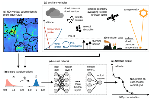
Figure 1Overview of the NitroNet model. Panels (a) and (b) depict the various input variables, which undergo feature transformation (c) before entering NitroNet's neural network (d). The output of the neural network is an NO2 profile on a vertical grid of the user's choice. PBL: planetary boundary layer. PBLH: planetary boundary layer height.
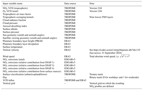
Table 1 gives an overview of all input variables (“features”) of the neural network. For the NO2 and O3 VCDs, the most recent TROPOMI product version (2.04) is used. Tropospheric averaging kernels (AKs) are computed according to Eskes et al. (2019) and defined on the vertical grid of the TM5 model. NitroNet uses the tropospheric AKs from the nine lowest TM5 layers (reaching up to ∼2300 m altitude), although it was later discovered that the AKs contribute only very little to the overall prediction quality, most likely due to redundancy with other input variables (cloud data, surface albedo, the sun zenith angle, etc.). The ERA5 variables “wind speed” and “vertical velocity” are vertically resolved at 1000, 950, 900, 850, 750, and 700 hPa. Wind speed refers to the absolute wind speed profile, i.e. , where u, and v are the northward and eastward wind speeds, respectively. “Boundary layer dissipation” is an ERA5 variable that measures the conversion of kinetic energy into heat due to small-scale eddies in the planetary boundary layer (PBL). NitroNet receives NOx emissions from the EDGARv5 emission inventory, along with the corresponding relative contributions of four emission bins based on the Selected Nomenclature for Air Pollution (SNAP; see European Environment Agency, 2023). The intent is to inform the neural network about the horizontal (EDGARv5) and vertical (SNAP) distributions of emissions. The SNAP sectors used here are “SNAP 1” (public power, cogeneration, and district heating plants), “SNAP 3” (industrial combustion), “SNAP 4” (production processes), and “surface emissions”, by which we refer to, for example, road traffic or agricultural emissions. NitroNet uses a ternary surface classification (urban, cropland, and forest classes), which is available within the TROPOMI NO2 product. The “VCD influx” variable represents the amount of NO2 that an observed TROPOMI pixel receives from its 8 immediate neighbouring pixels due to advection. The corresponding wind speeds are taken from the ERA5 reanalysis.

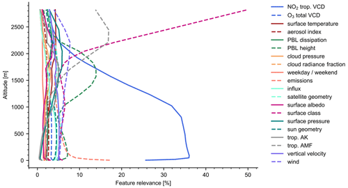
Figure 2Feature relevance analysis of the NitroNet model. The legend in the top-right corner indicates the data sources of the different input groups. Note that “trop.” stands for tropospheric.
An in-depth analysis of the feature importance of each input variable was conducted (see Fig. 2). The intention was to compute the relevance of each input variable for the model's prediction quality in a rigorous manner, using the so-called Shapley scores (see Štrumbelj and Kononenko, 2013). As expected, the NO2 VCD is by far the most important input feature (F=30.9 %), followed by the emission variables (F=8.9 %) and the PBLH (F=6.9 %). A detailed explanation and further interpretation are found in Appendix B.
3.2 Neural network design
NitroNet's neural network design is based on an extensive hyperparameter study (see Bergstra and Bengio, 2012), in which 300 different variants of the neural network (with different numbers of hidden layers, neurons per layer, training algorithms, etc.) were tested. The performance of a neural network can strongly depend on these parameters, but the parameters' ideal values cannot be determined from prior knowledge. The different variants were ranked based on their mean absolute percentage error (MAPE) on the validation set of WRF-2019. The MAPE is defined as
where N is the number of instances in the validation set, ypred is the neural network prediction, and ytrue is the ground truth. The best neural network with regard to this metric was chosen for NitroNet and is described in the following.
The neural network has eight hidden layers, each with 326 neurons, corresponding to approximately 850 000 trainable parameters. It uses the parametric rectified linear unit (PReLU) activation function (see He et al., 2015); the Nesterov Adam (Nadam) optimizer (see Ruder, 2016); a learning rate of ; a batch size of 2048; and the L1 loss function, defined as
In order to reduce early stagnation of the training process as a result of excessively large learning rates, a simple learning rate scheduler was used (ReduceLROnPlateau; see Paszke et al., 2019). The learning rate was halved whenever the training progress, as measured by the validation loss, stalled over several epochs (i.e. full iterations over the training set). Detailed information about the hyperparameter optimization procedure can be found in Appendix A. NitroNet further deploys feature transformations (e.g. the quantile transformation from the “sklearn” library; see Pedregosa et al., 2012) to reduce scale differences and skewness in the input variables. Feature transformations are known to improve the predictive capability of machine learning models, particularly when features or targets have a skewed or long-tailed distribution. This is the case for some of NitroNet's input features (e.g. the NO2 VCD). Likewise, transformations are applied to NitroNet's training targets (the NO2 concentrations at different altitudes; see e.g. Fig. C1). Prediction uncertainties are computed via the Monte Carlo method, for which a comprehensive summary is found in Anderson (1976). Figure 1 shows an overview of the NitroNet model.
3.3 Training NitroNet on filtered data
The overall performance of NitroNet can be significantly enhanced by the implementation of a filtering scheme for training data. The idea is to rank the NO2 profiles from WRF-2019 by their agreement with reference data and to only use the best few percent for training. More specifically, we define two thresholds, ΔVCD and ΔPBLH, and remove all training instances where
Here, VCDWRF denotes the simulated NO2 VCD from WRF-2019, VCDTROPOMI represents the observed NO2 VCD from TROPOMI (using the simulated NO2 a priori profiles), PBLHWRF denotes the simulated PBLH from WRF-2019, and PBLHERA5 represents the PBLH from ERA5. This way, profiles with poor agreement with the TROPOMI NO2 VCD (representing the total amount of NO2) or the ERA5 PBLH (representing the atmospheric mixing depth and profile shape) are identified and dismissed from the training. The lower the ΔVCD and ΔPBLH values chosen, the fewer the instances that remain in the training set. Therefore, we face a tradeoff between training data quality and quantity, which we resolve by including ΔVCD and ΔPBLH in the hyperparameter optimization mentioned in Sect. 3.2. In this way, ideal values of ΔVCD=0.2 and ΔPBLH=0.1 are determined. With these thresholds, only the best 7 % of all profiles (approximately 100 000) remain for training. Figure C2 gives an overview of the spatial distribution of NO2 VCDs after filtering and the fraction of remaining instances across the domain.
It should be mentioned that the TROPOMI NO2 VCD and the ERA5 PBLH are quantities with significant uncertainties. For the retrieval of the tropospheric NO2 VCD, the tropospheric air mass factor uncertainty (typically 20 %–50 %) is known to dominate the overall uncertainty in the column (typically 30 %–60 %; see e.g. Liu et al., 2021). Guo et al. (2024) report summertime ERA5 PBLH errors of approximately 150 m over continental regions, derived from radiosonde measurements. With an average PBLH of approx. 1500 m over the WRF-2019 domain, this amounts to a relative uncertainty of approx. 10 %.
However, caution is warranted: if the training dataset is manipulated in such a way, it may become unrepresentative of the real world (e.g. through the extinction of feature modes). Evaluation on the validation set shows that the use of filtered training data introduces a low bias of approximately −10 % to the NitroNet predictions in the lower layers of the atmosphere. This bias can be determined immediately after training, stored in an altitude-dependent lookup table, and automatically subtracted from NitroNet's predictions. From a machine learning perspective, this lookup table is simply another hyperparameter whose optimization is justified via validation on the independent test set.
3.4 Treatment of out-of-distribution instances
Neural networks are known to struggle when presented with out-of-distribution (OOD) instances, i.e. input data which lie outside the joint distribution of the training set. In the case of NitroNet (trained on 1 month of summertime RCT data in Europe), OOD instances are likely to occur in previously unseen geographical regions or seasons. The impact of OOD input variables on the neural network's performance can be detrimental, even if the neural network's sensitivity to the variable was low in the in-distribution case. In order to minimize the influence of OOD input variables, we implement a variant of the “winsorization” method (see e.g. Ruppert, 2014). First, the marginal probability density distributions () of the features (xi) are estimated using kernel density estimation (KDE) for the training set. Instance entries are considered OOD if they lie in regions of relatively low probability density, e.g. if . In such cases, they are replaced with a sample from . The NO2 VCD and categorical input features (i.e. surface classifications) are exempt from this treatment. The described method is applied exclusively at the time of prediction. The number of features affected depends mainly on the season and location of the input data.
3.5 Correction of NOz biases in the in situ measurements
An important part of the validation study presented in Sect. 4 will be the comparison of NitroNet predictions with in situ measurements at the surface. Over 90 % of the European in situ measurements rely on the molybdenum-based chemiluminescence method, which is demonstrably cross-sensitive to other atmospheric oxidants (summarized as “NOz”), such as peroxyacetyl nitrate (PAN), nitric acid (HNO3), and alkyl nitrates (see Dunlea et al., 2007; Steinbacher et al., 2007; Lamsal et al., 2008; Boersma et al., 2009; Villena et al., 2012). Consequently, the reported NO2 values are often too large because a fraction of the NOz is falsely registered as NO2. Lamsal et al. (2008) give an empirical formula for the overestimation of the NO2 concentration in the presence of NOz:
where [PAN], [HNO3], and [NO2] denote the true surface mixing ratios of PAN, HNO3, and NO2, while [] denotes the biased measurement result. The same formula was used in Kuhn et al. (2024) and was found to be crucial for the agreement between simulation data and in situ measurements. NitroNet was trained to predict F (as learned from WRF-2019) as an additional output, meaning that when comparing NitroNet predictions to in situ measurements, the measurement bias can be compensated for. Internally, this additional output is achieved by instantiating a second identical neural network, trained on the F targets from WRF-2019 instead of the NO2 targets. Because alkyl nitrates are not included in the MOZART chemical mechanism used in WRF-2019, we must assume that the sum of the alkyl nitrates is 0. According to Elshorbany et al. (2012), the contribution of the alkyl nitrates to F can be estimated to be in the range of 2 %–6 %. Based on the evaluation on the test set, NitroNet can reproduce the F values from WRF-2019 with a relative precision of ±5 % and no bias.
4.1 Evaluation of NitroNet in May 2019
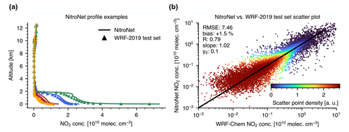
From hereon, we deal with the validation of the trained NitroNet model. The easiest way to confirm the successful training of the model is to validate it against new examples from the test set. Figure 3a shows four exemplary NO2 profiles from the test set and the corresponding predictions from NitroNet. Our model reproduces the shape and magnitude of the profiles well, although there are small deviations, e.g. in profile “C” at ∼ 3 km altitude. Within the boundary layer, almost no discrepancies are observed. A noteworthy feature of the NO2 profiles is their upper-tropospheric portion, starting at 8 km altitude. Here, a sudden enhancement of the NO2 concentration is found, which could be linked, for example, to aircraft emissions, the decay of NOx reservoirs, lightning, or stratosphere–troposphere exchange. Figure 3b shows a scatter plot of all NO2 concentrations in the (filtered) test set against their corresponding NitroNet predictions. The linear regression reveals excellent agreement, a strong correlation of R=0.99, and a negligible bias of −0.4 %. The relative prediction errors are smaller at higher NO2 concentrations. This is because the high NO2 concentrations at the surface are more strongly correlated with the NO2 VCD, which is the main model input. Conversely, the correlation is weaker in higher layers, where the concentration tends to be lower. Therefore, the combined input variables are more descriptive of the lower, more polluted layers and allow the neural network to make a more precise prediction. Note that Fig. 3 shows data from the filtered test set exclusively. This choice was made for two main reasons. On one hand, we aim to exclude supposedly erroneous NO2 profiles from WRF-Chem for the evaluation of NitroNet. These profiles would result in larger errors in the comparison between WRF-Chem and NitroNet, particularly because the WRF-Chem NO2 profiles show systematic errors that NitroNet does not reproduce. This is demonstrated more explicitly further below. On the other hand, the evaluation against filtered test data is an assessment of the neural network's performance in isolation; i.e. it indicates its prediction errors for instances from the same distribution as the training set. For completeness, a version of Fig. 3 based on unfiltered test data is shown in Fig. C3.
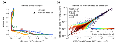
Figure 3Evaluation of NitroNet on the WRF-2019 test set. (a) Four exemplary NO2 profiles from the test set (triangular markers) with corresponding NitroNet predictions (solid lines). (b) Scatter plot of all NO2 concentrations from the test set vs. their corresponding NitroNet predictions. The RMSE and intercept are expressed in units of . Note that “conc.” stands for concentration and “a.u.” stands for arbitrary units.
Next, we verify that training on filtered data, as described in Sect. 3.3, does indeed have the desired effect. For this purpose, we intercompare observed and simulated NO2 VCDs and surface concentrations from WRF-2019, NitroNet, TROPOMI, and AirBase.
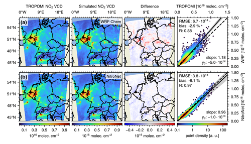
Figure 4Comparison of monthly-mean TROPOMI NO2 VCDs against simulated NO2 VCDs from WRF-Chem (a) and NitroNet (b) (May 2019). The NO2 a priori profiles used in the air mass factor computation of the TROPOMI VCDs were replaced with those from WRF-Chem and NitroNet, respectively. The RMSE and intercept are given in units of .
Figure 4a shows the comparison of monthly-mean NO2 VCDs from TROPOMI and the corresponding simulation results from WRF-2019. The simulated VCDs are computed as
where l denotes the layer index, ltp represents the tropopause layer index, cl represents the NO2 concentration in layer l, and Δhl represents the vertical extent of layer l. The NO2 a priori profiles used in the air mass factor computation of the TROPOMI VCDs were replaced with those from WRF-Chem, following Eskes et al. (2019):
where VCDobs, corr denotes the VCD with the exchanged a priori profile, VCDobs denotes the original VCD, AMF represents the total air mass factor, AMFtrop represents the tropospheric air mass factor, and Al denotes the tropospheric averaging kernel of layer l. Figure 4a reveals significant biases in the WRF-Chem simulation of up to (e.g. in western Germany, northern Austria, and the Kaliningrad Oblast). The simulated and observed NO2 VCDs agree with a mean bias of −2.9 %, a root-mean-squared error (RMSE) of , and a correlation coefficient of R=0.88. Here, and throughout the rest of the article, “correlation coefficient” refers to the Pearson correlation coefficient. A more detailed discussion of the WRF-Chem simulation results can be found in Kuhn et al. (2024).
Figure 4b shows the same comparison but uses the NO2 profiles from NitroNet instead of WRF-Chem. Overall, much better agreement is observed. In particular, the major overestimations observed with WRF-Chem have disappeared, while some weak underestimations remain. Although the absolute mean bias is slightly larger (−8.1 %), the correlation is much stronger (R=0.97), and the RMSE is almost halved (). In some regions of the domain (e.g. near the cities of Frankfurt and Mannheim, Germany), these improvements are easily explained by the considerable reduction in the simulated column. In other regions (e.g. at the border between Belgium, the Netherlands, and Germany), the improvements must be partially attributed to larger TROPOMI reference VCDs, resulting from the use of presumably more realistic a priori NO2 profiles. Because the NO2 VCD is the dominant input variable of NitroNet and acts essentially as a scaling factor for the predicted NO2 profiles, the relative prediction uncertainty is approximately equal to that of the NO2 VCD (here, 30 %–60 %).
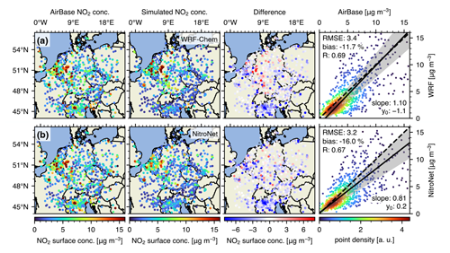
Figure 5Comparison of monthly-mean AirBase NO2 surface observations against simulated surface concentrations from WRF-Chem (a) and NitroNet (b) at the TROPOMI overpass time (May 2019). The AirBase observations were corrected for NOz biases using WRF-Chem model results in panel (a) and NitroNet predictions in panel (b), respectively. The RMSE and intercept are given in units of µg m−3.
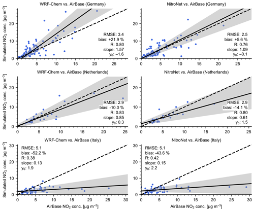
Figure 5 shows a comparison of monthly-mean NO2 surface concentrations from AirBase with the corresponding model results from the time of the TROPOMI overpass. The NOz bias correction described in Sect. 3.5 was applied to the AirBase data using WRF-2019 and NitroNet model results for instruments using the chemiluminescence method with a molybdenum converter. The “difference” plots in Figs. 4 and 5 show a clear correlation, e.g. with regard to western Germany and northern Italy. Nonetheless, different spatial patterns can be identified between NitroNet and WRF-2019: in some model regions (e.g. in western Germany), NitroNet produced smaller errors than WRF-Chem with respect to the VCDs and the surface concentrations. However, the opposite is observed in other regions. For example, NitroNet produced smaller VCD errors but larger surface concentration errors in northern Italy. This demonstrates that filtering the training data based on VCD and PBLH criteria alone may not always lead to better neural network predictions at the surface. Scatter plots for individual countries (Germany, the Netherlands, and Italy) with differing responses to the data filtering (improvement, neutral response, or worsening) can be found in Figs. C4 and C5. This finding is important for the interpretation of the presented results: WRF-Chem produces positive and negative errors in moderate balance, while NitroNet produces similar negative but much smaller positive errors. Accordingly, NitroNet shows a smaller RMSE (3.2 vs. 3.4 µg m−3) but a larger absolute mean bias (−16.0 % vs. −11.7 %). In such a case, the increase in absolute mean bias is obviously not a suitable measure for overall model skill. The slight reduction in the correlation coefficient (R=0.67 vs. R=0.69) escapes this argument but can be considered insignificant.
Figure 6 shows a histogram of the NOz biases in the in situ measurements, computed from modelled PAN and HNO3 mixing ratios according to Lamsal et al. (2008) (see Sect. 3.5). The results obtained from WRF-Chem and NitroNet show values of up to +200 %. We show this figure with the intent of emphasizing that caution is required when using in situ measurements for the training and validation of RCT and machine learning models without a proper correction strategy. As mentioned before, NitroNet is able to reproduce the NOz correction factors of WRF-Chem with a relative precision of ±5 % and no bias. Due to the good agreement between WRF-Chem and NitroNet in this regard, the prediction of the NOz correction factors cannot explain the low biases observed in Fig. 5.
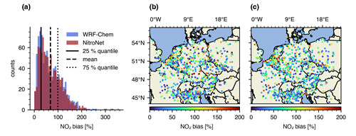
Figure 6Panel (a) presents a histogram, while panels (b) and (c) show geographic distributions of the monthly-mean NOz biases from WRF-Chem and NitroNet, respectively. All panels correspond to the AirBase observations shown in Fig. 5.
The results in this section demonstrate that our training method has had its intended effect: when using filtered data, NitroNet produces NO2 profiles with an overall more realistic magnitude and/or shape than WRF-Chem. Although the improvement in the simulated surface concentrations is rather small, a much stronger improvement in the VCDs is obtained. Even better results are expected from further filtering the training data based on their agreement with the in situ observations. However, this is impossible here as the surface observations are so sparse that too little data would remain for training the neural network.
4.2 Evaluation of NitroNet on unseen data (May 2022)
We now address the validation of NitroNet using completely new input data from the month of May 2022. From hereon, we use NitroNet without any comparison to RCT simulation data, evaluating it over a domain ranging from 44° N to 56° N and from 2° W to 23° E.
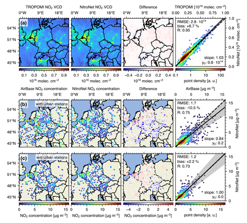
Figure 7Comparison of monthly-mean TROPOMI NO2 VCDs (a) and AirBase surface observations (b) against NitroNet predictions (May 2022). Panel (c) is identical to panel (b) except that AirBase instruments classified as “urban background” have been removed. The RMSE and intercept are displayed in molec. cm−2 for the VCDs and in µg m−3 for the surface concentrations. Note that “w/o” stands for without.
4.2.1 Validation against TROPOMI satellite data and AirBase in situ measurements
Figure 7 shows a comparison of monthly-mean NO2 VCDs from TROPOMI against NitroNet predictions. The computations were conducted as explained in Sect. 4.1. The NitroNet NO2 VCDs show magnitudes, geographical distributions, and errors similar to those from May 2019. However, the results for May 2022 show a lower RMSE (2.8×10¹⁴ vs. 3.8×10¹⁴ ) and an increased mean bias (+6.7 % vs. −8.1 %). This apparent improvement could be purely coincidental: Fig. 4b indicates a slight underestimation of the NO2 VCDs by NitroNet. On the other hand, the NO2 VCDs for May 2019 are on average 18 % higher than those for May 2022. Consequently, NitroNet may overestimate the true VCDs because it attempts to reproduce the approximate magnitudes learned from 2019. If the two effects cancel each other out, this could reasonably explain the smaller VCD errors observed in 2022.
Figure 7b shows a comparison of monthly-mean NO2 surface concentrations from AirBase against NitroNet predictions. NitroNet correctly identifies surface pollution hotspots (e.g. in Paris (France), Essen (Germany), and Hamburg (Germany)) but somewhat underestimates surface NO2 concentrations in various regions of the domain. Compared to May 2019, the results show a smaller mean bias (−10.5 % vs. −16.0 %), a higher correlation coefficient (R=0.75 vs. R=0.67), and a significantly reduced RMSE (1.7 vs. 3.2 µg m−3). A key contribution to these differences is found in the Lombardy region of northern Italy. Here, significant underestimations were observed in 2019, but the corresponding data points are missing entirely for 2022. Inspection of the AirBase metadata reveals that in May 2019, over 92 % of the Italian measurements were flagged as “valid”, 5 % were flagged as “invalid”, and 2 % were flagged as “below the detection limit”. In May 2022, however, only 48 % of the measurements were flagged as valid, 13 % were flagged as invalid, and 39 % were flagged as below the detection limit. Additionally, the total number of Italian instruments was reduced from 320 in 2019 to just 69 in 2022. It remains unclear why these measurements were removed from AirBase.
Another interesting observation is the dependence of NitroNet's low bias on the measuring stations' type. Here, we refer to the entire domain shown in Fig. 7. As explained in Sect. 2.2, we exclusively use background stations throughout our study, based on the argument that accurate modelling of traffic and industrial scenarios is known to require simulations with a much higher resolution (local scale). So far, we have assumed no errors in the classification of the AirBase instruments. However, based on the resolutions of modern emission inventories, the variability in trace gas transport, and the scarce documentation of classification criteria, it can be argued that the category “urban background” is a grey zone within this classification. After all, emission inventories clearly show that urban regions are always affected by traffic emissions. Furthermore, Fig. 7 shows significant low biases in NitroNet's surface predictions but no corresponding low biases in the tropospheric columns. This can partly be attributed to the interpixel variability in the TROPOMI measurements. Surface stations with a large NitroNet bias are possibly located closer to strong traffic emissions and thus are less correlated with the NO2 VCD, which acts as the main model input. We therefore investigated whether the comparison of NitroNet's results to in situ observations would improve by removing the urban background stations, as shown in Fig. 7c. Significant improvements were revealed, manifesting in increased slopes (from 0.84 to 1.00), a lower absolute mean bias (−10.5 % to +2.2 %), and a lower RMSE (1.7 to 1.2 µg m−3). These improvements can be explained either by a tendency of NitroNet to underestimate NO2 concentrations in urban areas or by an ambiguous categorization of the measurements. Due to the lack of information about the classification process, we will omit the urban background stations from our evaluations from hereon.
4.2.2 Validation against FRM4DOAS MAX-DOAS measurements
We now validate the NO2 profiles from NitroNet against MAX-DOAS measurements from the FRM4DOAS dataset with respect to six European locations. A temporal threshold of 60 min is used, meaning that each NitroNet NO2 profile is associated with the average of all colocated MAX-DOAS profiles recorded within 60 min of the corresponding satellite overpass. Averaging kernels are available from the MMF retrieval algorithm and are given as an n×n matrix (A), where n denotes the number of vertical layers in the retrieval. The ith row of A describes the retrieval sensitivity of the concentration value of layer i to the other n layers. An ideal retrieval would be characterized by A=𝟙, where 𝟙 denotes the unity matrix. In practice, the AK matrix diagonal is usually close to unity at the surface but quickly drops below 50 % within the first 1–2 km above ground (see e.g. Fig. C7, which shows the AK matrix of the instrument in Heidelberg, Germany). The AKs are applied to the NitroNet profiles following Rodgers (2000) and thus by computing
where csim denotes the original NitroNet profile and cap represents the assumed a priori profile. The AKs are applied as described when comparing NitroNet to the MMF profiles. MAPA, on the other hand, does not provide AKs.
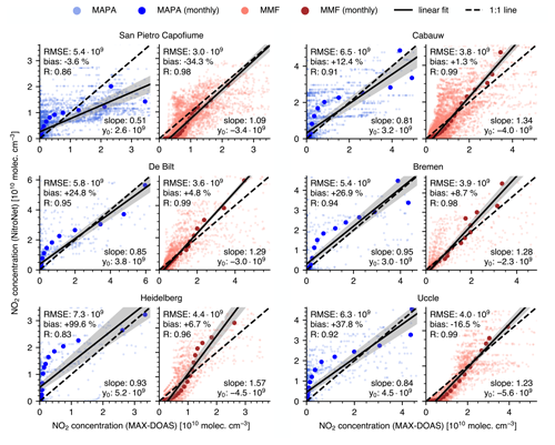
Figure 8Comparison of FRM4DOAS NO2 concentrations against NitroNet predictions (May 2022). MAPA results are shown in blue, and MMF results are shown in red. Faint scatter points represent a one-to-one comparison of NO2 concentration values (i.e. the concentrations of individual profiles). Bold scatter points indicate the monthly-mean NO2 concentrations of the retrieval layers. The RMSE and intercept are displayed in molec. cm−3 and were computed based on the monthly-mean scatter points.
Figure 8 shows the results obtained with this procedure. The faint scatter points (“MAPA” and “MMF” in the legend) represent a one-to-one comparison of NO2 concentration values from NitroNet and MAPA/MMF. The bold scatter points (“MAPA (monthly)” and “MMF (monthly)” in the legend) show the monthly-mean NO2 concentrations of each retrieval layer.
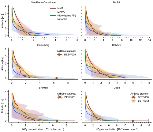
Figure 9Comparison of monthly-mean FRM4DOAS NO2 profiles against NitroNet profiles (May 2022). Monthly standard deviations of the profiles are shown as shaded regions in the background. Where available, colocated AirBase measurements of surface NO2 concentrations within a radius of 5 km are shown at 0 m altitude.
The level of agreement between FRM4DOAS and NitroNet varies depending on the instrument location. NitroNet and MAPA show significant differences in some locations, with biases ranging from −3.6 % (San Pietro Capofiume) to +99.6 % (Heidelberg), RMSE values on the scale of 6×10⁹ molec. cm−3, and correlation coefficients ranging from R=0.86 (San Pietro Capofiume) to R=0.95 (De Bilt). NitroNet and MMF show overall better agreement, with biases ranging from −34.3 % (San Pietro Capofiume) to +8.7 % (Bremen), RMSE values on the scale of 4×10⁹ , and correlation coefficients larger than 0.90. The linear regressions show significantly steeper slopes for MMF than for MAPA but show similar intercepts. MAPA tends to produce higher NO2 concentrations than MMF in the lowest few hundred metres above ground but lower concentrations at higher altitudes. The NitroNet predictions are somewhere in between, resulting in an S-shaped distribution of the scatter markers (see e.g. the comparison to MMF for Heidelberg). The corresponding plots of monthly-mean NO2 profiles can be found in Fig. 9. Additionally, colocated measurements from in situ measurements (within a radius of 5 km) are included in the corresponding plots in Fig. 9. NitroNet shows good agreement with the surface observations (except for the station “BETR012” in Uccle). This is made possible by NitroNet's high vertical resolution at the surface (∼1 m), which is adequate for capturing the steep prevailing concentration gradients. This is not the case for MAPA and MMF because the vertical sampling of FRM4DOAS (∼200 m) is too coarse. Our observations in this regard align well with the findings of Bösch (2018), who presents a detailed comparison of MAX-DOAS measurements and colocated surface observations. The differences between MAPA, MMF, and NitroNet can partly be linked to the models' implementations and limitations: MMF uses a single, fixed NO2 a priori profile for all retrievals, which was obtained from a WRF-Chem simulation in Mexico (Friedrich et al., 2019). However, datasets like our WRF-2019 show strong horizontal variability in NO2 profiles on scales of just a few kilometres. A single a priori profile is therefore not sufficient to fully represent the diversity of profile shapes and magnitudes. Moreover, horizontal gradients also systematically affect the MAX-DOAS profile retrievals. Accordingly, it is not surprising to see larger differences between MMF, MAPA, and NitroNet (without AKs) in regions of reduced sensitivity (small AKs) above 1 km altitude. Application of the AKs reduces the differences significantly in three out of the six locations (De Bilt, Cabauw, and Bremen). MAPA, on the other hand, makes a priori assumptions in the form of a pre-defined profile parametrization. The profiles shown in Fig. 9 are qualitatively similar to those from MAPA's original publication (Beirle et al., 2019), with a strong exponential shape and an optional peak in the second or third layer (San Pietro Capofiume and Cabauw). This could indicate the presence of an elevated NO2 layer. NitroNet is unable to reproduce this profile type, most likely because the training dataset contains very few corresponding examples. As shown in Kuhn et al. (2024), the WRF-Chem model, which provides NitroNet’s training data, also struggles to reproduce elevated layers in some locations. However, the elevated layers are also not reproduced by MMF. In that regard, it is possible that they are falsely produced by an incompatibility between the true NO2 profile and MAPA's profile parametrization (technically a form of model misspecification error). Overall, the differences between MAPA and MMF demonstrate the large uncertainty resulting solely from the choice of retrieval algorithm. Further hard-to-quantify sources of uncertainty (e.g. the influence of horizontal gradients), as well as the low statistical relevance of only using six measurement locations, must also be considered. Within these limitations, the comparison with MAX-DOAS data shows no glaring discrepancies, although it allows for no more than an approximate validation of profile shapes and magnitudes.
4.3 Evaluation of NitroNet in other seasons and regions of the world
Lastly, we present an analysis of NitroNet's ability to generalize to other seasons and regions of the world. The evaluations shown in Sect. 4.2.1 were made for the same region (central Europe) and time of the year (May) on which the neural network was trained. Hence, they represent the least challenging test case. Good generalization to other domains and seasons is not guaranteed and is associated with two challenges. Firstly, the neural network must respond reasonably to fundamentally different input data (e.g. much lower temperatures in winter than in summer). This is controlled by the network's regularization, which we enforce mainly via the winsorization technique described in Sect. 3.4. Secondly, the training data are expected to be “epistemically incomplete”, meaning they do not contain all relevant training examples for other seasons and regions. This is a property of the training set, which we regard as a principal limitation that cannot be resolved in the scope of this article. Nonetheless, it is not implausible that the fundamental relationships between the input and output data, as learned by NitroNet, hold at least partly for other seasons and regions as well.
We first investigate the regional generalization capability of the model using reference data from May 2022. Figure 10 shows a comparison with TROPOMI NO2 VCDs over the United Kingdom (UK; Fig. 10a) and the Mediterranean region of Portugal and Spain (Fig. 10b). The results are overall very similar to those from the central European domain investigated previously. However, Fig. 10b shows significant overestimations of approximately 1015 molec. cm−2 over the southern waterbodies (the Alboran Sea and the Gulf of Cádiz). It is not generally unexpected to see such systematic errors in the predictions of a neural network. The most likely explanation is that the training dataset does not contain enough representative examples of NO2 profiles over water. The water regions in the training set must be assumed to be less representative because, for example, they are pervaded by an unusually high number of shipping routes, which may lead NitroNet to overestimate NO2 over more remote waterbodies. We exclude these pixels from the statistical analysis because they skew the results over the landmasses on which we aim to validate NitroNet in this article. Compared to the central European domain, the RMSE values increase from 2.8×10¹⁴ molec. cm−2 to 3.3×10¹⁴ molec. cm−2 (UK) and 3.1×10¹⁴ molec. cm−2 (Spain and Portugal), while the correlation coefficients decrease from R=0.95 to R=0.92 (UK) and R=0.86 (Spain and Portugal). The mean biases are +12.3 % (UK) and +3.4 % (Spain and Portugal). For context, an RMSE of 5.0×10¹⁴ molec. cm−2, a bias of +18.0 %, and a correlation coefficient of R=0.74 are obtained for the domain of Spain and Portugal if water pixels are included. The statistical analysis of the UK domain, however, is practically unaffected by water pixels.
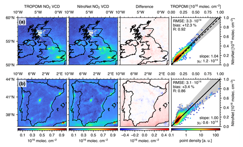
Figure 10As in Fig. 7a but for (a) the UK and (b) Spain and Portugal. Water pixels are shown as grey dots in the right-hand scatter plots and are excluded from the statistical analysis. The RMSE and intercept are displayed in molec. cm−2.
Figure 11 shows a corresponding comparison to AirBase surface observations, in analogy to Fig. 7, including the omission of urban background stations. A version of Fig. 11 including urban stations can be found in Fig. C6. The results are similar: for the UK domain, the RMSE slightly increases from 1.2 to 1.8 µg m−3, and the correlation coefficient significantly decreases from R=0.73 to R=0.45. This is caused by the two outliers in the southeastern corner of the domain and is amplified by the low number of total observations. For the Mediterranean domain, the number of observations is much larger, and the results are overall better, with an RMSE of 1.6 µg m−3 and a correlation coefficient of R=0.71. This demonstrates that NitroNet can generalize to new but qualitatively similar domains with a minor loss of prediction accuracy.
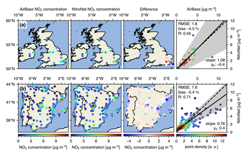
Figure 11As in Fig. 7c but for (a) the UK and (b) Spain and Portugal. The RMSE and intercept are displayed in µg m−3.
NitroNet was also tested on three more distant domains covering the United States (US) West Coast, India, and western China (see Fig. 12). We obtain good agreement for the US West Coast (an RMSE of 2.7×10¹⁴ molec. cm−2, a bias of +2.7 %, and R=0.84). The Indian domain shows stronger correlation but lower accuracy due to significant overestimations (an RMSE of = 8.0×10¹⁴ molec. cm−2, a bias of +41.5 %, and R=0.91). The biggest deviations and weakest correlations are observed over the Chinese domain (an RMSE of 12.6×10¹⁴ molec. cm−2, a bias of +12.5 %, and R=0.70). Here, as shown in Fig. 12c, NitroNet ignores entire pollution hotspot areas in the northern Shanxi and Shaanxi provinces. These regions are known for their strong emissions from coal, steel, chemical, and military industries (see e.g. Peng et al., 2023). China's rapid economic development, combined with its fewer environmental state regulations, makes it plausible that the EDGARv5 emission data from the year 2015 might already be outdated in such locations. Besides, NitroNet may struggle with the differences in atmospheric composition, e.g. the vastly higher aerosol pollution levels that prevail in China (see e.g. Meng et al., 2022). The previously mentioned overestimation over waterbodies is observed in all three domains.
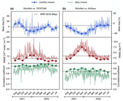
Finally, we investigate the seasonal performance of NitroNet. For this purpose, data covering a whole year (August 2021–July 2022) were processed for the central European domain. The NitroNet predictions were evaluated against TROPOMI and AirBase observations, and time series of the bias, RMSE, and correlation coefficient were computed (see Fig. 13). Shown here are daily-mean values, as well as monthly-mean values, in analogy to the other evaluations presented up to this point. Note that in this context, monthly-mean bias refers to the bias computed on monthly means as opposed to the monthly mean of daily biases (which can be estimated from the daily values shown in Fig. 13). The same holds for the RMSE and the correlation coefficient. Because averaging over multiple days reduces the noisiness of the NitroNet predictions, the monthly-mean RMSE values are smaller, and the correlation coefficients larger, than those for unaveraged data. The mean biases, however, are unaffected by averaging. In the following, we will focus on the monthly means. NitroNet's performance shows a clear seasonal cycle: the mean biases increase during wintertime and reach maximal values of −22.4 % (compared to TROPOMI in January) and −50.1 % (compared to AirBase in December). Likewise, the RMSE increases during wintertime and reaches maximal values of 10.8×10¹⁴ molec. cm−2 (compared to TROPOMI in January) and 6.3 µg m−3 (compared to AirBase in December). The correlation coefficients are on the scale of R≈0.90 (compared to TROPOMI) and R≈0.70 (compared to AirBase), with no conclusive annual cycle. The decrease in model performance in winter is expected due to the reasons discussed earlier. In particular, the oxidative capacity (via hydroxyl and peroxy radicals) is reduced in winter, resulting in increased NO2 lifetimes of more than 20 h, as opposed to 2–6 h in summer (see e.g. Liu et al., 2016; Shah et al., 2020). The results show that without specifically training on wintertime data, NitroNet's predictions for deep winter are only of limited value. Besides the obvious challenge of achieving good generalization from summertime training data to wintertime predictions, higher uncertainties in the input satellite data should also be taken into account in this context (see e.g. Douros et al., 2023). Nonetheless, compared to the typical performance of RCT simulations, NitroNet performs well for the majority of the analysed time series. Compared to WRF-2019, with equivalent filter criteria, the RMSE values of NitroNet's NO2 VCDs and surface concentrations are lower in 9 out of 12 months. It should be noted that the performance of RCT simulations is also expected to drop significantly in wintertime. The scientific literature on the topic is sparse, but a study by Douros et al. (2023) shows that CAMS (an ensemble model consisting of 11 RCT models) produces summertime VCD biases of ∼15 % and wintertime VCD biases of ∼50 % in Europe. In light of such results, NitroNet's seasonal performance on the European domain can be considered competitive compared to most of the recent RCT simulations. Figure C8 shows examples of the comparison between NitroNet and TROPOMI for 2 individual days in summer and winter. In contrast to the monthly-mean comparisons shown previously, the data contain a significant number of gaps (e.g. due to clouds), the correlation is reduced (R≈0.80), and the prediction errors are larger. This is expected since averaging over an entire month of data reduces the statistical noise of the model. Nonetheless, as reflected in Fig. 13, NitroNet's daily performance is still competitive compared to that of WRF-Chem, indicating that it can reasonably be used for unaveraged predictions. A version of Fig. 13 with urban stations included is found in Fig. C9.
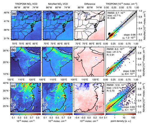
Figure 12As in Fig. 10 but for (a) the US West Coast, (b) India, and (c) western China. The grey scatter markers in panel (a) symbolize entries over water, which were excluded from the statistical analysis.
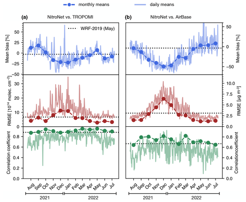
Figure 13Seasonal evaluation of NitroNet over the central European domain against (a) NO2 VCDs from TROPOMI and (b) surface observations from AirBase. The dotted grey line, “WRF-2019 (May)”, indicates the value of the statistical diagnostics (i.e. the mean bias, RMSE, and correlation coefficient) obtained from WRF-2019 for comparison.
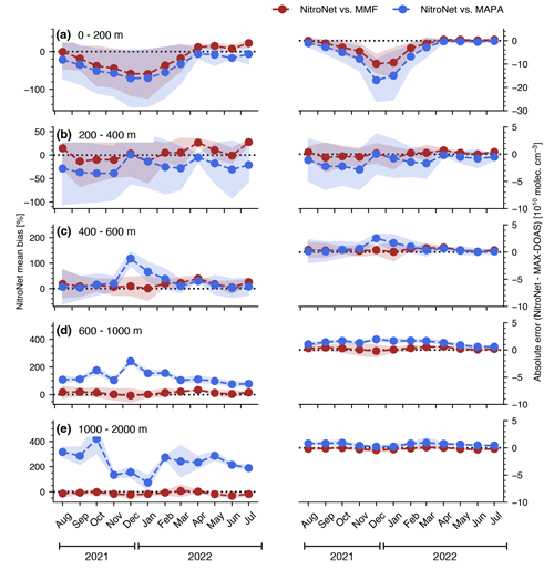
Figure 14Seasonal evaluation of NitroNet against NO2 concentrations from the FRM4DOAS dataset. Shown here are NitroNet's monthly-mean biases and absolute errors averaged over all available MAX-DOAS instruments in the selected altitude ranges: (a) 0–200 m, (b) 200–400 m, (c) 400–600 m, (d) 600–1000 m, and (e) 1000–2000 m.
Figure 14 shows a full-year evaluation of NitroNet against NO2 concentrations from FRM4DOAS in selected altitude ranges. For this analysis, NitroNet’s average bias (left panels) and absolute error (right panels) over all previously shown FRM4DOAS instruments were computed for a full year of data, with either MMF or MAPA used as reference. Each panel of Fig. 14 is restricted to a specific altitude range (0–200 m, 200–400 m, 400–600 m, 600–1000 m, and 1000–2000 m). In the lowest evaluation layer, at 0–200 m, there is particularly good agreement between MAPA and MMF, with NitroNet biases between −70 % and +20 % over the course of the year. Here, a tendency similar to that in Fig. 13 can be observed, with low biases occurring during winter and high biases during summer. The summertime high biases are of a magnitude similar to that of the biases in the comparison with TROPOMI VCDs and AirBase surface measurements (approximately +15 % vs. +23 % and +10 %, respectively). Particularly in the higher layers, the validation against MMF yields far lower mean biases, mostly in the range of −30 % to +30 %, while the validation against MAPA results in larger biases of 100 % at 600–1000 m and 200 % at 1000–2000 m. This is owing to the steeper vertical concentration gradients of the MAPA profiles, due to their assumed profile shape, and aligns well with the profiles shown in Fig. 9. The large relative biases of NitroNet in relation to MAPA might appear concerning at first and should be put into perspective based on the following considerations.
First, it is hard to assess which of the two retrieval algorithms yields more trustworthy results. Although conceptually different, MAPA and MMF both suffer from increasingly poor sensitivity at higher altitudes. This is also the case here, as exemplified by the MMF averaging kernels shown in Fig. C7, which indicate an effective vertical sensitivity of up to 1.5 km in Heidelberg (May 2022). As a consequence, the retrieval results are considerably affected by a priori assumptions. In the case of MMF, an a priori profile is taken from a WRF-Chem simulation over Mexico (see Friedrich et al., 2019), which might be entirely unrepresentative of the central European domain investigated here. Parametrized retrievals, such as MAPA,do not require a priori profiles, which is an advantage in this context. Nonetheless, MAPA still depends on other a priori assumptions, e.g. in the form of the assumed profile shape determined by the choice of parametrization. In particular, the exponential tail of the MAPA profiles at higher altitudes, which is the dominant characteristic here, is prescribed.
Second, computing the relative biases of NitroNet involves dividing the absolute errors by the NO2 concentrations of MMF or MAPA. In the case of MAPA, these can be considerably small (e.g. molec. cm−3 for 1000–2000 m; see Fig. 9 for reference) for the reasons discussed above. Thereby, even moderate absolute errors (see the right-hand panels of Fig. 14) can result in large relative biases. Thus, the assessment of model performance by means of the prediction biases is informative in the lowest three evaluation layers (up to 600 m) but not beyond.
Another important finding from Fig. 14 is that the seasonal trends observed in Fig. 13 are represented in the lowest layer (0–200 m) but not in the higher ones. This indicates that the seasonal biases of NitroNet (and the underlying WRF-Chem training data) might be rooted in the lower regions of the troposphere.
In this article, we have introduced NitroNet, a new deep learning NO2 profile retrieval prototype for TROPOMI. NitroNet is trained on 1 month of RCT simulation data from the WRF-Chem model for central Europe (May 2019). The use of synthetic data allows us to overcome several obstacles associated with the empirical datasets used in other studies. The main benefits of our approach can be summarized as follows:
-
Because measurements of NO2 profiles are still sparse, empirical training data are effectively restricted to surface in situ observations. A synthetic training dataset allows the neural network to learn the prediction of full NO2 profiles instead. These training profiles also cover the spatial domain continuously and might cover scenarios that escape the in situ observations altogether due to the strategic placement of the instruments.
-
The NO2 in situ measurements used in empirical training sets contain a hidden NOz bias of typically >20 % due to cross-sensitivities to atmospheric oxidants. Without access to model data, this bias cannot be corrected and is silently reproduced by other neural networks.
-
The abundance of training data from the RCT simulation allows for the generous dismissal of untrustworthy training examples without running into a data shortage. We can therefore train the neural network on filtered data that have been purged of erroneous example profiles. The neural network can then exceed the prediction quality of the original RCT simulation.
The latter concept of learning from the good examples but dismissing the errors of a data-generating model has been explored in other publications (e.g. Sayeed et al., 2023; Li et al., 2023), although in a somewhat different context. These publications describe the development of synergistic neural-network–RCT combination models, while NitroNet is designed for standalone use as a surrogate model for the computationally expensive and slow RCT simulations. To put this into perspective, using 800 CPUs, it took ∼5 d to produce 1 month of WRF-Chem simulation data, while NitroNet can process the same amount of data in just ∼20 min using 31 GPUs, with obvious operational advantages. Nevertheless, this functionality is limited to the prediction of NO2 profiles, and NitroNet cannot be considered a full replacement for RCT simulations, which can predict the concentrations of many other trace gases and aerosols, as well as meteorological variables.
Our main results were reported in Sect. 4.2 in the form of an extensive evaluation of the NitroNet model. Three observational datasets (NO2 VCDs from TROPOMI, background in situ observations from AirBase, and NO2 profiles from FRM4DOAS) were used as monthly-mean reference data. First, an intercomparison between NitroNet, WRF-Chem, TROPOMI, and AirBase was performed for May 2019. Hereby, the benefits of training the neural network on filtered data were demonstrated. NitroNet showed far better agreement with TROPOMI NO2 VCDs than WRF-Chem did, while the comparison with AirBase surface observations returned similar results for both models. The NOz cross-sensitivities of the in situ measurements were estimated based on modelled PAN and HNO3 mixing ratios, resulting in significant bias correction factors of up to +200 %.
Next, NitroNet was evaluated on previously unseen data from May 2022. The comparison with TROPOMI NO2 VCDs showed a strong correlation of R=0.95, a bias of +6.7 %, and an RMSE of 2.8×10¹⁴ molec. cm−2. The comparison with FRM4DOAS NO2 profiles showed good agreement when using the MMF retrieval algorithm (RMSE molec. cm−3) and slightly worse results when using the MAPA retrieval (RMSE ≈ 6×10⁹ molec. cm−3). The comparison with AirBase surface observations resulted in a correlation of R=0.75, a bias of −10.5 %, and an RMSE of 1.7 µg m−3. By omitting the instruments categorized as urban background, the bias and RMSE were reduced to +2.2 % and 1.2 µg m−3, respectively.
Lastly, the model evaluation was extended to different seasons (August 2021–July 2022 for the central European domain) and regions of the Earth (UK, Spain and Portugal, the US West Coast, India, and China for May 2022). Over the UK, Spain and Portugal, and the US West Coast, NitroNet performed similarly to how it did over the original central European training domain. Over India and China, larger deviations and weaker correlations were found. The strongest differences occurred in the heavily industrialized regions of northern China, where the emission data used as model input might have been outdated. In all domains (except for the UK), NitroNet consistently overestimated the NO2 load over waterbodies by approximately 1015 molec. cm−2. The seasonal analysis revealed stable model performance in spring, summer, and early autumn (March–September) but exhibited significant low biases in surface concentrations of up to −50 % during late autumn and winter (October–February). Part of these underestimations may be attributed to the higher uncertainties in the main model input, the NO2 VCD, during wintertime.
In closing this article, we give an outlook on future improvements and use cases for NitroNet. We will attempt to produce a full year of synthetic training data, possibly in more diverse geographical regions. This will result in more consistent model accuracy across different seasons and regions of the world. In particular, it might also help to resolve the prediction errors over water, which could be useful in addressing some of the outstanding research questions related to NO2 over oceans (e.g. those concerning the contribution of ship emissions and lightning to the lower/upper troposphere). Similarly, NitroNet could benefit from training data with a higher horizontal resolution, which might improve its ability to reproduce more complex NO2 profile shapes, e.g. ones with elevated layers. Until then, NitroNet should be considered a prototype. Furthermore, the inclusion of more data from new instruments will strongly influence the training and validation of future model versions. Here, the most promising outlook is the advent of geostationary satellites, such as the Geostationary Environmental Monitoring Spectrometer (GEMS; see Kim et al., 2020), “Tropospheric Emissions: Monitoring of Pollution” (TEMPO; see Naeger et al., 2021), and Sentinel-4 (see Stark et al., 2013). These will provide hourly resolved NO2 columns, allowing for the implementation of diurnal cycles into our model. The use of more intricate MAX-DOAS retrieval algorithms could allow for better sensitivity to higher layers of the troposphere (see e.g. Schofield et al., 2004, who achieved sensitivity to the stratosphere and upper troposphere with a zenith-sky viewing geometry). NO2 profile observations from cloud slicing (see e.g. Marais et al., 2021) or aircraft measurements (see e.g. Riess et al., 2023; Brenninkmeijer et al., 2007) may be used for further validation of NitroNet at various altitudes. The ongoing efforts in harmonizing observational datasets (see e.g. the GHOST dataset; Bowdalo et al., 2024) will allow for easier model validation at the surface in all regions of the Earth. In particular, they might open up new possibilities for including valuable information from surface in situ measurements into NitroNet. Previous studies have reported on neural networks trained directly on in situ observations (see e.g. Gardner and Dorling, 1999; Kang et al., 2021; Chan et al., 2021; Ghahremanloo et al., 2021; Zhang et al., 2022; Jesemann et al., 2022; Cao, 2023). NitroNet aims to overcome the aforementioned disadvantages associated with empirical training targets by using synthetic training data instead. Nonetheless, information from in situ measurements could be included implicitly by using it as an additional criterion in the data-filtering procedure. This results in significantly smaller training sets because the European in situ observations are sparse compared to the satellite measurements. Such limitations could be overcome by extending the regional model's spatio-temporal domain or through neural network training methods specifically designed for sparse training data (e.g. via data augmentation). Lastly, more complex neural network designs, such as invertible neural networks (INNs; see Ardizzone et al., 2018), or physically informed neural networks (PINNs; see Raissi et al., 2019) may be implemented once the remaining parts of the project are deemed mature enough. This is motivated by recent advancements in machine-learning-based weather forecasting (e.g. the Aurora model, based on vision transformers and encoder–decoder mechanisms; see Bodnar et al., 2024). The NitroNet model can be used for scientific research, such as that concerning the following:
-
a revision of existing studies on near-surface air pollution and the associated effects on human health, with explicit treatment of the NOz biases in in situ measurements;
-
reprocessing of the TROPOMI NO2 columns by replacing the poorly resolved NO2 a priori profiles from the TM5 model (horizontal resolution: 1° × 1°) with the significantly better-resolved NO2 profiles from NitroNet (horizontal resolution: 3.5 km×5.5 km);
-
possibly predicting other trace gas profiles, such as SO2 or HCHO.
Altogether, the combined efforts of machine learning, RCT modelling, and instrumental development hold promising potential for the near future.
The hyperparameter study for NitroNet is based on 300 different model versions. The model configurations were sampled randomly (“random search”; see Bergstra and Bengio, 2012). An overview of the hyperparameters and their respective sampling ranges can be found in Table A1.
Table A1Overview of NitroNet's hyperparameters. ReLU: rectified linear unit. CELU: continuously differentiable exponential linear unit. GELU: Gaussian error linear unit. SELU: scaled exponential linear unit. MSE: mean square error. RMSLE: root mean square logarithmic error.
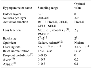
For a full reference of these terms, see Schmidhuber (2015) and Paszke et al. (2019). 1 See the PyTorch documentation (https://pytorch.org/docs/stable/generated/torch.nn.SmoothL1Loss.html). 2 See the PyTorch documentation (https://pytorch.org/docs/stable/generated/torch.optim.AdamW.html). 3 The original range was 0–0.5, but training diverged for runs with a drop-out probability > 0.15. 4 See Sect. 3.3.
Stochastic gradient descent (SGD) was not used because all training runs using SGD diverged. The Adam optimizer was found to be outclassed by Nadam and AdamW early on and was subsequently omitted from the study. Figure A1 shows the results of the hyperparameter study in a parallel coordinate view. The validation MAPE, which is used as a performance metric to compare the model configurations, ranges from ∼10 %–30 %. This demonstrates that a hyperparameter search can potentially improve the neural network's performance by up to a factor of 3, making it an essential step in the development of NitroNet.
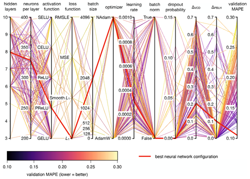
Figure A1Results of the hyperparameter study in a parallel coordinate view. Each hyperparameter is represented by one vertical axis (“hidden layers”, “neurons per layer”, etc.). Each variant of the neural network is represented by a contiguous line that intersects the vertical axes at the network's hyperparameter values. The last vertical axis shows the MAPE achieved for the validation set, which serves as the metric for the selection of the best neural network configuration (lower values are better). The optimal configuration is shown as a thick red line. Note that “batch norm” stands for batch normalization.
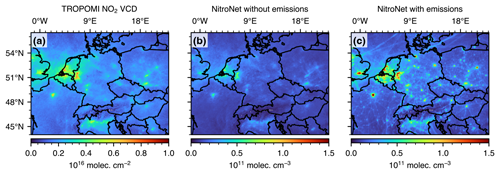
Figure B2Demonstration of the relevance of the emissions feature group. Panel (a) shows the monthly-mean NO2 VCD from TROPOMI (May 2019). Panels (b) and (c) show the corresponding NO2 surface concentrations from NitroNet, with all emissions turned off and on, respectively.
In order to gain more insight into how the neural network of NitroNet operates, a feature relevance analysis was conducted. The goal was to quantify how strongly each input variable contributes to the overall model performance. The standard method involves computing the Shapley scores of the input variables (see Shapley, 1951). The Shapley score of the ith input variable (xi) is defined as
where P denotes the set of all input variables and denotes the set cardinality. Moreover, is a function of choice, which acts as a measure for model performance by comparing the ground truth (ytrue) with the model's predictions (ypred) either by using all input variables (i.e. ) or by omitting the variable xi (i.e. I=S). Omission of the input variable xi is simulated by replacing its values with random samples from the validation set (approximating a sample drawn from the prior probability distribution of xi.). The feature relevance Fi is obtained by normalizing the Shapley scores, i.e. . The following further premises were made:
-
We define
meaning we use a scaled RMSE to measure model performance. The uninformed case (omitting all input variables; I=∅) equates to a model performance of f=0, and the fully informed case (omitting none of the input variables; I=P) equates to a model performance of f=1. Accordingly, all Shapley scores lie in the interval [0, 1].
-
Because the sum in Eq. (B1) iterates over a power set of large cardinality, not all summands can be evaluated. Instead, Ri is approximated by computing random summands of Eq. (B1) until the overall distribution of the feature relevances has converged.
-
Certain input variables are grouped together (e.g. the group “wind” contains all wind speed variables and does not discriminate between the u and v directions).
The feature relevance can also be computed separately for each vertical layer. The resulting feature relevance profiles are shown in Fig. B1. We draw the following conclusions:
-
The NO2 VCD is generally the most important input variable from 0 to 1500 m altitude.
-
The feature relevance of the PBLH peaks at ∼ 1800 m, which corresponds to the average PBLH value in WRF-2019. Because the NO2 profiles show strong gradients at the top of the PBLH, this feature relevance profile shape is expected.
-
The NO2 concentrations above the PBL are known to be low and weakly correlated with satellite observations. Here, the model performance is dominated by the input groups “surface class” and “tropospheric AMF”, which the neural network most likely uses to predict average NO2 profile estimates based on coarse general constraints (e.g. “over water”, “rural land”, and “urban land”).
-
At the surface, there is a tradeoff between the feature relevance of emission data and the NO2 VCD. This confirms that emission data are a valuable addition to NitroNet as they can improve model performance by almost 20 %.
The feature relevance of the emission data is further demonstrated in Fig. B2. Comparing Fig. B2a and b shows that when no emission data are used, NitroNet's prediction of the NO2 surface concentration is essentially proportional to the NO2 VCD. Once emissions are added as input (see Fig. B2c), the distribution of predicted surface concentrations becomes significantly more complex: high values suddenly occur despite the presence of comparably low VCDs (e.g. in the cities of Hamburg and Berlin, Germany), and fine-scale infrastructure, such as car highways connecting cities, becomes visible.
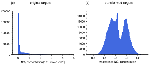
Figure C1Example of the data transformations used during the training of NitroNet. Shown here are histograms of the training targets (NO2 concentrations) at all altitudes before (a) and after (b) the application of a logarithmic data transformation. The transformed targets are unitless.
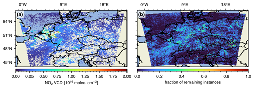
Figure C2Overview of the TROPOMI NO2 VCDs (with recomputed air mass factors) following the application of the data filter described in Sect. 3.3. Panel (a) shows the remaining data, averaged across all orbits from May 2019. Panel (b) shows the remaining fraction of instances in relation to the unfiltered dataset.
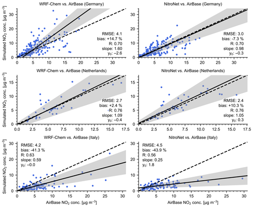
Figure C4Scatter plots of the data shown in Fig. 5, restricted to individual countries (Germany, the Netherlands, and Italy).
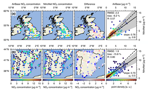
Figure C6As in Fig. 11 but with urban stations included. The RMSE and intercept are displayed in µg m−3.
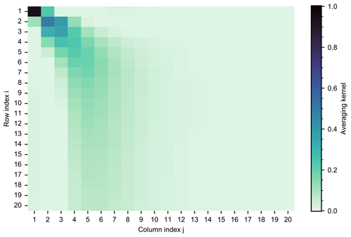
Figure C7Monthly-mean averaging kernel matrix from the FRM4DOAS instrument for Heidelberg (May 2022). The rows and columns are ordered such that index 1 represents the lowest layer of the retrieval, while index 20 represents the highest. Each layer has a vertical extent of 200 m.
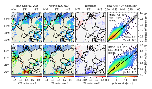
Figure C8As in Fig. 7a but for 1 summer day and 1 winter day. Panel (a) shows data from 5 May 2022. Panel (b) shows data from 5 November 2021.
All data are available from the authors upon reasonable request.
LK developed the research question under the supervision of TW and SB. LK, SO, and AP produced the training data for the neural network. LK wrote the text and produced the remaining content of the article, with all authors contributing by revising it interactively.
At least one of the (co-)authors is a member of the editorial board of Atmospheric Measurement Techniques. The peer-review process was guided by an independent editor, and the authors also have no other competing interests to declare.
Publisher’s note: Copernicus Publications remains neutral with regard to jurisdictional claims made in the text, published maps, institutional affiliations, or any other geographical representation in this paper. While Copernicus Publications makes every effort to include appropriate place names, the final responsibility lies with the authors.
We acknowledge Vinod Kumar for his invaluable help with RCT modelling, which preceded this article. We thank Andreas Richter, Udo Frieß, Ankie Piters, Michel van Roozendael, Alexis Merlaud, Elisa Castelli, and Paolo Pettinari for maintaining the MAX-DOAS instruments and sharing their data within the FRM4DOAS network. The FRM4DOAS project is funded by the European Space Agency (ESA) under contract no. 4000118181/16/I-EF. Data analysis and visualization were performed using the Python programming language, including the libraries “NumPy”, “SciPy”, “pandas”, “Xarray”, “Matplotlib”, and “cartopy”. The neural network for NitroNet was implemented using the PyTorch package.
The article processing charges for this open-access publication were covered by the Max Planck Society.
This paper was edited by Robyn Schofield and reviewed by Robert Ryan and one anonymous referee.
Anderson, G.: Error propagation by the Monte Carlo method in geochemical calculations, Geochim. Cosmochim. Acta, 40, 1533–1538, https://doi.org/10.1016/0016-7037(76)90092-2, 1976. a
Ardizzone, L., Kruse, J., Wirkert, S., Rahner, D., Pellegrini, E. W., Klessen, R. S., Maier-Hein, L., Rother, C., and Köthe, U.: Analyzing Inverse Problems with Invertible Neural Networks, https://doi.org/10.48550/ARXIV.1808.04730, 2018. a
Beckwith, M., Bates, E., Gillah, A., and Carslaw, N.: NO2 hotspots: Are we measuring in the right places?, Atmos. Environ. X, 2, 100025, https://doi.org/10.1016/j.aeaoa.2019.100025, 2019. a
Beirle, S., Dörner, S., Donner, S., Remmers, J., Wang, Y., and Wagner, T.: The Mainz profile algorithm (MAPA), Atmos. Meas. Tech., 12, 1785–1806, https://doi.org/10.5194/amt-12-1785-2019, 2019. a, b, c
Bergstra, J. and Bengio, Y.: Random Search for Hyper-Parameter Optimization, J. Mach. Learn. Res., 13, 281–305, 2012. a, b
Berkhout, A., Gast, L., van der Hoff, G., Swart, D., Hoed, M., and Allaart, M.: Atmospheric NO2 profiles measured with lidar during the CINDI-2 campaign, EPJ Web of Conferences, 176, 10002, https://doi.org/10.1051/epjconf/201817610002, 2018. a
Bieser, J., Aulinger, A., Matthias, V., Quante, M., and van der Gon, H.: Vertical emission profiles for Europe based on plume rise calculations, Environ. Pollut., 159, 2935–2946, https://doi.org/10.1016/j.envpol.2011.04.030, 2011. a
Bodnar, C., Bruinsma, W., Lucic, A., Stanley, M., Brandstetter, J., Garvan, P., Riechert, M., Weyn, J., Dong, H., Vaughan, A., Gupta, J., Thambiratnam, K., Archibald, A., Heider, E., Welling, M., Turner, R., and Perdikaris, P.: Aurora: A Foundation Model of the Atmosphere, Tech. Rep. MSR-TR-2024-16, Microsoft Research AI for Science, https://www.microsoft.com/en-us/research/publication/aurora-a-foundation-model-of-the-atmosphere/ (last access: 21 September 2024), 2024. a
Boersma, K. F., Jacob, D. J., Trainic, M., Rudich, Y., DeSmedt, I., Dirksen, R., and Eskes, H. J.: Validation of urban NO2 concentrations and their diurnal and seasonal variations observed from the SCIAMACHY and OMI sensors using in situ surface measurements in Israeli cities, Atmos. Chem. Phys., 9, 3867–3879, https://doi.org/10.5194/acp-9-3867-2009, 2009. a, b
Bourgeois, I., Peischl, J., Neuman, J. A., Brown, S. S., Allen, H. M., Campuzano-Jost, P., Coggon, M. M., DiGangi, J. P., Diskin, G. S., Gilman, J. B., Gkatzelis, G. I., Guo, H., Halliday, H. A., Hanisco, T. F., Holmes, C. D., Huey, L. G., Jimenez, J. L., Lamplugh, A. D., Lee, Y. R., Lindaas, J., Moore, R. H., Nault, B. A., Nowak, J. B., Pagonis, D., Rickly, P. S., Robinson, M. A., Rollins, A. W., Selimovic, V., St. Clair, J. M., Tanner, D., Vasquez, K. T., Veres, P. R., Warneke, C., Wennberg, P. O., Washenfelder, R. A., Wiggins, E. B., Womack, C. C., Xu, L., Zarzana, K. J., and Ryerson, T. B.: Comparison of airborne measurements of NO, NO2, HONO, NOy, and CO during FIREX-AQ, Atmos. Meas. Tech., 15, 4901–4930, https://doi.org/10.5194/amt-15-4901-2022, 2022. a
Bowdalo, D., Basart, S., Guevara, M., Jorba, O., Pérez García-Pando, C., Jaimes Palomera, M., Rivera Hernandez, O., Puchalski, M., Gay, D., Klausen, J., Moreno, S., Netcheva, S., and Tarasova, O.: GHOST: a globally harmonised dataset of surface atmospheric composition measurements, Earth Syst. Sci. Data, 16, 4417–4495, https://doi.org/10.5194/essd-16-4417-2024, 2024. a
Brenninkmeijer, C. A. M., Crutzen, P., Boumard, F., Dauer, T., Dix, B., Ebinghaus, R., Filippi, D., Fischer, H., Franke, H., Frieβ, U., Heintzenberg, J., Helleis, F., Hermann, M., Kock, H. H., Koeppel, C., Lelieveld, J., Leuenberger, M., Martinsson, B. G., Miemczyk, S., Moret, H. P., Nguyen, H. N., Nyfeler, P., Oram, D., O'Sullivan, D., Penkett, S., Platt, U., Pupek, M., Ramonet, M., Randa, B., Reichelt, M., Rhee, T. S., Rohwer, J., Rosenfeld, K., Scharffe, D., Schlager, H., Schumann, U., Slemr, F., Sprung, D., Stock, P., Thaler, R., Valentino, F., van Velthoven, P., Waibel, A., Wandel, A., Waschitschek, K., Wiedensohler, A., Xueref-Remy, I., Zahn, A., Zech, U., and Ziereis, H.: Civil Aircraft for the regular investigation of the atmosphere based on an instrumented container: The new CARIBIC system, Atmos. Chem. Phys., 7, 4953–4976, https://doi.org/10.5194/acp-7-4953-2007, 2007. a
Bösch, T.: Detailed analysis of MAX-DOAS measurements in Bremen: Spatial and temporal distribution of aerosols, formaldehyde and nitrogen dioxide, Ph.D. thesis, Universität Bremen, http://nbn-resolving.de/urn:nbn:de:gbv:46-00107093-11 (last access: 21 September 2024), 2018. a
Cao, E. L.: National ground-level NO2 predictions via satellite imagery driven convolutional neural networks, Front. Environ. Sci., 11, https://doi.org/10.3389/fenvs.2023.1285471, 2023. a, b
Chan, K. L., Khorsandi, E., Liu, S., Baier, F., and Valks, P.: Estimation of Surface NO2 Concentrations over Germany from TROPOMI Satellite Observations Using a Machine Learning Method, Remote Sens., 13, 969, https://doi.org/10.3390/rs13050969, 2021. a, b
Chowdhury, S., Haines, A., Klingmüller, K., Kumar, V., Pozzer, A., Venkataraman, C., Witt, C., and Lelieveld, J.: Global and national assessment of the incidence of asthma in children and adolescents from major sources of ambient NO2, Environ. Res. Lett., 16, 035020, https://doi.org/10.1088/1748-9326/abe909, 2021. a
Crippa, M., Guizzardi, D., Oreggioni, G., Muntean, M., and Schaaf, E.: EDGARv5.0 Air Pollutant Emissions, Pangaea [data set], https://doi.org/10.1594/PANGAEA.921922, 2020. a
Douros, J., Eskes, H., van Geffen, J., Boersma, K. F., Compernolle, S., Pinardi, G., Blechschmidt, A.-M., Peuch, V.-H., Colette, A., and Veefkind, P.: Comparing Sentinel-5P TROPOMI NO2 column observations with the CAMS regional air quality ensemble, Geosci. Model Dev., 16, 509–534, https://doi.org/10.5194/gmd-16-509-2023, 2023. a, b, c, d, e
Dunlea, E. J., Herndon, S. C., Nelson, D. D., Volkamer, R. M., San Martini, F., Sheehy, P. M., Zahniser, M. S., Shorter, J. H., Wormhoudt, J. C., Lamb, B. K., Allwine, E. J., Gaffney, J. S., Marley, N. A., Grutter, M., Marquez, C., Blanco, S., Cardenas, B., Retama, A., Ramos Villegas, C. R., Kolb, C. E., Molina, L. T., and Molina, M. J.: Evaluation of nitrogen dioxide chemiluminescence monitors in a polluted urban environment, Atmos. Chem. Phys., 7, 2691–2704, https://doi.org/10.5194/acp-7-2691-2007, 2007. a, b
Elshorbany, Y. F., Steil, B., Brühl, C., and Lelieveld, J.: Impact of HONO on global atmospheric chemistry calculated with an empirical parameterization in the EMAC model, Atmos. Chem. Phys., 12, 9977–10000, https://doi.org/10.5194/acp-12-9977-2012, 2012. a
Emmons, L. K., Schwantes, R. H., Orlando, J. J., Tyndall, G., Kinnison, D., Lamarque, J.-F., Marsh, D., Mills, M. J., Tilmes, S., Bardeen, C., Buchholz, R. R., Conley, A., Gettelman, A., Garcia, R., Simpson, I., Blake, D. R., Meinardi, S., and Pétron, G.: The Chemistry Mechanism in the Community Earth System Model Version 2 (CESM2), J. Adv. Model. Earth Syst., 12, 4, https://doi.org/10.1029/2019ms001882, 2020. a
Eskes, H., van Geffen, J., Sneep, M., Apituley, A., and Veefkind, J.: Sentinel-5 precursor/TROPOMI Level 2 Product User Manual Nitrogendioxide, Royal Netherlands Meteorological Institute, https://sentinels.copernicus.eu/web/sentinel/data-products/-/asset_publisher/fp37fc19FN8F/content/sentinel-5-precursor-level-2-nitrogen-dioxide (last access: 21 September 2024), 2019. a, b, c
European Environment Agency: EMEP/EEA air pollutant emission inventory guidebook 2023, Publications Office of the European Environment Agency, https://doi.org/10.2800/795737, 2023. a
European Environment Agency: Air Quality e-Reporting [Data Set], https://www.eea.europa.eu/data-and-maps/data/aqereporting-8 (last access: 10 March 2024), 2024. a, b
Faustini, A., Rapp, R., and Forastiere, F.: Nitrogen dioxide and mortality: review and meta-analysis of long-term studies, European Respiratory Journal, European Respiratory Society (ERS), 44, 744–753, https://doi.org/10.1183/09031936.00114713, 2014. a
Fayt, C., Friedrich, M., and Hendrick, F.: Fiducial Reference Measurements for Ground-Based DOAS Air-Quality Observations, Royal Belgian Institute for Space Aeronomy, https://frm4doas.aeronomie.be/ProjectDir/FRM4DOAS_CCN02_D20_MAXDOAS_Network_Operational_Processing_System_Architecture_Design_Document__v2.0_20210903.pdf (last access: 21 September 2024), 2021. a
Friedrich, M. M., Rivera, C., Stremme, W., Ojeda, Z., Arellano, J., Bezanilla, A., García-Reynoso, J. A., and Grutter, M.: NO2 vertical profiles and column densities from MAX-DOAS measurements in Mexico City, Atmos. Meas. Tech., 12, 2545–2565, https://doi.org/10.5194/amt-12-2545-2019, 2019. a, b, c
Gardner, M. and Dorling, S.: Neural network modelling and prediction of hourly NOx and NO2 concentrations in urban air in London, Atmos. Environ., 33, 709–719, https://doi.org/10.1016/S1352-2310(98)00230-1, 1999. a, b
Ghahremanloo, M., Lops, Y., Choi, Y., and Yeganeh, B.: Deep Learning Estimation of Daily Ground‐Level NO2 Concentrations From Remote Sensing Data, J. Geophys. Res.-Atmos., 126, https://doi.org/10.1029/2021jd034925, 2021. a, b
Grell, G. A., Peckham, S. E., Schmitz, R., McKeen, S. A., Frost, G., Skamarock, W. C., and Eder, B.: Fully coupled “online” chemistry within the WRF model, Atmos. Environ., 39, 6957–6975, https://doi.org/10.1016/j.atmosenv.2005.04.027, 2005. a, b
Guo, J., Zhang, J., Shao, J., Chen, T., Bai, K., Sun, Y., Li, N., Wu, J., Li, R., Li, J., Guo, Q., Cohen, J. B., Zhai, P., Xu, X., and Hu, F.: A merged continental planetary boundary layer height dataset based on high-resolution radiosonde measurements, ERA5 reanalysis, and GLDAS, Earth Syst. Sci. Data, 16, 1–14, https://doi.org/10.5194/essd-16-1-2024, 2024. a
He, K., Zhang, X., Ren, S., and Sun, J.: Delving Deep into Rectifiers: Surpassing Human-Level Performance on ImageNet Classification, https://doi.org/10.48550/ARXIV.1502.01852, 2015. a
Hersbach, H., Bell, B., Berrisford, P., Hirahara, S., Horányi, A., Muñoz-Sabater, J., Nicolas, J., Peubey, C., Radu, R., Schepers, D., Simmons, A., Soci, C., Abdalla, S., Abellan, X., Balsamo, G., Bechtold, P., Biavati, G., Bidlot, J., Bonavita, M., De Chiara, G., Dahlgren, P., Dee, D., Diamantakis, M., Dragani, R., Flemming, J., Forbes, R., Fuentes, M., Geer, A., Haimberger, L., Healy, S., Hogan, R. J., Hólm, E., Janisková, M., Keeley, S., Laloyaux, P., Lopez, P., Lupu, C., Radnoti, G., de Rosnay, P., Rozum, I., Vamborg, F., Villaume, S., and Thépaut, J.-N.: The ERA5 global reanalysis, Q. J. Roy. Meteorol. Soc., 146, 1999–2049, https://doi.org/10.1002/qj.3803, 2020. a
Hönninger, G., von Friedeburg, C., and Platt, U.: Multi axis differential optical absorption spectroscopy (MAX-DOAS), Atmos. Chem. Phys., 4, 231–254, https://doi.org/10.5194/acp-4-231-2004, 2004. a
Ialongo, I., Virta, H., Eskes, H., Hovila, J., and Douros, J.: Comparison of TROPOMI/Sentinel-5 Precursor NO2 observations with ground-based measurements in Helsinki, Atmos. Meas. Tech., 13, 205–218, https://doi.org/10.5194/amt-13-205-2020, 2020. a
Jesemann, A.-S., Matthias, V., Böhner, J., and Bechtel, B.: Using Neural Network NO2-Predictions to Understand Air Quality Changes in Urban Areas – A Case Study in Hamburg, Atmosphere, 13, 1929, https://doi.org/10.3390/atmos13111929, 2022. a, b
Kang, Y., Choi, H., Im, J., Park, S., Shin, M., Song, C.-K., and Kim, S.: Estimation of surface-level NO2 and O3 concentrations using TROPOMI data and machine learning over East Asia, Environ. Pollut., 288, 117711, https://doi.org/10.1016/j.envpol.2021.117711, 2021. a, b
Kerkweg, A. and Jöckel, P.: The 1-way on-line coupled atmospheric chemistry model system MECO(n) – Part 1: Description of the limited-area atmospheric chemistry model COSMO/MESSy, Geosci. Model Dev., 5, 87–110, https://doi.org/10.5194/gmd-5-87-2012, 2012. a
Kim, J., Jeong, U., Ahn, M.-H., Kim, J. H., Park, R. J., Lee, H., Song, C. H., Choi, Y.-S., Lee, K.-H., Yoo, J.-M., Jeong, M.-J., Park, S. K., Lee, K.-M., Song, C.-K., Kim, S.-W., Kim, Y. J., Kim, S.-W., Kim, M., Go, S., Liu, X., Chance, K., Miller, C. C., Al-Saadi, J., Veihelmann, B., Bhartia, P. K., Torres, O., Abad, G. G., Haffner, D. P., Ko, D. H., Lee, S. H., Woo, J.-H., Chong, H., Park, S. S., Nicks, D., Choi, W. J., Moon, K.-J., Cho, A., Yoon, J., kyun Kim, S., Hong, H., Lee, K., Lee, H., Lee, S., Choi, M., Veefkind, P., Levelt, P. F., Edwards, D. P., Kang, M., Eo, M., Bak, J., Baek, K., Kwon, H.-A., Yang, J., Park, J., Han, K. M., Kim, B.-R., Shin, H.-W., Choi, H., Lee, E., Chong, J., Cha, Y., Koo, J.-H., Irie, H., Hayashida, S., Kasai, Y., Kanaya, Y., Liu, C., Lin, J., Crawford, J. H., Carmichael, G. R., Newchurch, M. J., Lefer, B. L., Herman, J. R., Swap, R. J., Lau, A. K. H., Kurosu, T. P., Jaross, G., Ahlers, B., Dobber, M., McElroy, C. T., and Choi, Y.: New Era of Air Quality Monitoring from Space: Geostationary Environment Monitoring Spectrometer (GEMS), B. Am. Meteorol. Soc., 101, E1–E22, https://doi.org/10.1175/bams-d-18-0013.1, 2020. a
Krol, M., Houweling, S., Bregman, B., van den Broek, M., Segers, A., van Velthoven, P., Peters, W., Dentener, F., and Bergamaschi, P.: The two-way nested global chemistry-transport zoom model TM5: algorithm and applications, Atmos. Chem. Phys., 5, 417–432, https://doi.org/10.5194/acp-5-417-2005, 2005. a, b
Kuhn, L., Beirle, S., Kumar, V., Osipov, S., Pozzer, A., Bösch, T., Kumar, R., and Wagner, T.: On the influence of vertical mixing, boundary layer schemes, and temporal emission profiles on tropospheric NO2 in WRF-Chem – comparisons to in situ, satellite, and MAX-DOAS observations, Atmos. Chem. Phys., 24, 185–217, https://doi.org/10.5194/acp-24-185-2024, 2024. a, b, c, d, e, f
Kuik, F., Lauer, A., Churkina, G., Denier van der Gon, H. A. C., Fenner, D., Mar, K. A., and Butler, T. M.: Air quality modelling in the Berlin–Brandenburg region using WRF-Chem v3.7.1: sensitivity to resolution of model grid and input data, Geosci. Model Dev., 9, 4339–4363, https://doi.org/10.5194/gmd-9-4339-2016, 2016. a
Kuik, F., Kerschbaumer, A., Lauer, A., Lupascu, A., von Schneidemesser, E., and Butler, T. M.: Top–down quantification of NOx emissions from traffic in an urban area using a high-resolution regional atmospheric chemistry model, Atmos. Chem. Phys., 18, 8203–8225, https://doi.org/10.5194/acp-18-8203-2018, 2018. a
Lamsal, L. N., Martin, R. V., van Donkelaar, A., Steinbacher, M., Celarier, E. A., Bucsela, E., Dunlea, E. J., and Pinto, J. P.: Ground-level nitrogen dioxide concentrations inferred from the satellite-borne Ozone Monitoring Instrument, J. Geophys. Res.-Atmos., 113, D16, https://doi.org/10.1029/2007JD009235, 2008. a, b, c, d
Lange, K., Richter, A., Schönhardt, A., Meier, A. C., Bösch, T., Seyler, A., Krause, K., Behrens, L. K., Wittrock, F., Merlaud, A., Tack, F., Fayt, C., Friedrich, M. M., Dimitropoulou, E., Van Roozendael, M., Kumar, V., Donner, S., Dörner, S., Lauster, B., Razi, M., Borger, C., Uhlmannsiek, K., Wagner, T., Ruhtz, T., Eskes, H., Bohn, B., Santana Diaz, D., Abuhassan, N., Schüttemeyer, D., and Burrows, J. P.: Validation of Sentinel-5P TROPOMI tropospheric NO2 products by comparison with NO2 measurements from airborne imaging DOAS, ground-based stationary DOAS, and mobile car DOAS measurements during the S5P-VAL-DE-Ruhr campaign, Atmos. Meas. Tech., 16, 1357–1389, https://doi.org/10.5194/amt-16-1357-2023, 2023. a, b
Li, B., Hu, Q., Gao, M., Liu, T., Zhang, C., and Liu, C.: Physical informed neural network improving the WRF-CHEM results of air pollution using satellite-based remote sensing data, Atmos. Environ., 311, 120031, https://doi.org/10.1016/j.atmosenv.2023.120031, 2023. a
Liu, F., Beirle, S., Zhang, Q., Dörner, S., He, K., and Wagner, T.: NOx lifetimes and emissions of cities and power plants in polluted background estimated by satellite observations, Atmos. Chem. Phys., 16, 5283–5298, https://doi.org/10.5194/acp-16-5283-2016, 2016. a
Liu, S., Valks, P., Pinardi, G., Xu, J., Chan, K. L., Argyrouli, A., Lutz, R., Beirle, S., Khorsandi, E., Baier, F., Huijnen, V., Bais, A., Donner, S., Dörner, S., Gratsea, M., Hendrick, F., Karagkiozidis, D., Lange, K., Piters, A. J. M., Remmers, J., Richter, A., Van Roozendael, M., Wagner, T., Wenig, M., and Loyola, D. G.: An improved TROPOMI tropospheric NO2 research product over Europe, Atmos. Meas. Tech., 14, 7297–7327, https://doi.org/10.5194/amt-14-7297-2021, 2021. a, b
Manders, A. M. M., Builtjes, P. J. H., Curier, L., Denier van der Gon, H. A. C., Hendriks, C., Jonkers, S., Kranenburg, R., Kuenen, J. J. P., Segers, A. J., Timmermans, R. M. A., Visschedijk, A. J. H., Wichink Kruit, R. J., van Pul, W. A. J., Sauter, F. J., van der Swaluw, E., Swart, D. P. J., Douros, J., Eskes, H., van Meijgaard, E., van Ulft, B., van Velthoven, P., Banzhaf, S., Mues, A. C., Stern, R., Fu, G., Lu, S., Heemink, A., van Velzen, N., and Schaap, M.: Curriculum vitae of the LOTOS–EUROS (v2.0) chemistry transport model, Geosci. Model Dev., 10, 4145–4173, https://doi.org/10.5194/gmd-10-4145-2017, 2017. a
Marais, E. A., Roberts, J. F., Ryan, R. G., Eskes, H., Boersma, K. F., Choi, S., Joiner, J., Abuhassan, N., Redondas, A., Grutter, M., Cede, A., Gomez, L., and Navarro-Comas, M.: New observations of NO2 in the upper troposphere from TROPOMI, Atmos. Meas. Tech., 14, 2389–2408, https://doi.org/10.5194/amt-14-2389-2021, 2021. a, b, c
Meng, F., Zhang, Y., Kang, J., Heal, M. R., Reis, S., Wang, M., Liu, L., Wang, K., Yu, S., Li, P., Wei, J., Hou, Y., Zhang, Y., Liu, X., Cui, Z., Xu, W., and Zhang, F.: Trends in secondary inorganic aerosol pollution in China and its responses to emission controls of precursors in wintertime, Atmos. Chem. Phys., 22, 6291–6308, https://doi.org/10.5194/acp-22-6291-2022, 2022. a
Menut, L., Bessagnet, B., Briant, R., Cholakian, A., Couvidat, F., Mailler, S., Pennel, R., Siour, G., Tuccella, P., Turquety, S., and Valari, M.: The CHIMERE v2020r1 online chemistry-transport model, Geosci. Model Dev., 14, 6781–6811, https://doi.org/10.5194/gmd-14-6781-2021, 2021. a
Mills, I. C., Atkinson, R. W., Kang, S., Walton, H., and Anderson, H. R.: Quantitative systematic review of the associations between short-term exposure to nitrogen dioxide and mortality and hospital admissions, BMJ Open, https://doi.org/10.1136/bmjopen-2014-006946, 2015. a
Naeger, A. R., Newchurch, M. J., Moore, T., Chance, K., Liu, X., Alexander, S., Murphy, K., and Wang, B.: Revolutionary Air-Pollution Applications from Future Tropospheric Emissions: Monitoring of Pollution (TEMPO) Observations, B. Am. Meteorol. Soc., 102, E1735–E1741, https://doi.org/10.1175/bams-d-21-0050.1, 2021. a
Paszke, A., Gross, S., Massa, F., Lerer, A., Bradbury, J., Chanan, G., Killeen, T., Lin, Z., Gimelshein, N., Antiga, L., Desmaison, A., Kopf, A., Yang, E., DeVito, Z., Raison, M., Tejani, A., Chilamkurthy, S., Steiner, B., Fang, L., Bai, J., and Chintala, S.: PyTorch: An Imperative Style, High-Performance Deep Learning Library, Adv. Neural Info. Process. Syst., 32, 8024–8035, https://proceedings.neurips.cc/paper_files/paper/2019/file/bdbca288fee7f92f2bfa9f7012727740-Paper.pdf (last access: 21 September 2024), 2019. a, b
Pedregosa, F., Varoquaux, G., Gramfort, A., Michel, V., Thirion, B., Grisel, O., Blondel, M., Müller, A., Nothman, J., Louppe, G., Prettenhofer, P., Weiss, R., Dubourg, V., Vanderplas, J., Passos, A., Cournapeau, D., Brucher, M., Perrot, M., and Duchesnay, E.: Scikit-learn: Machine Learning in Python, https://doi.org/10.48550/ARXIV.1201.0490, 2012. a
Peng, S., Giron, C., Liu, G., d’Aspremont, A., Benoit, A., Lauvaux, T., Lin, X., de Almeida Rodrigues, H., Saunois, M., and Ciais, P.: High-resolution assessment of coal mining methane emissions by satellite in Shanxi, China, iScience, 26, 108375, https://doi.org/10.1016/j.isci.2023.108375, 2023. a
Platt, U. and Stutz, J.: Differential Optical Absorption Spectroscopy, Springer Berlin Heidelberg, https://doi.org/10.1007/978-3-540-75776-4, 2008. a, b
Poraicu, C., Müller, J.-F., Stavrakou, T., Fonteyn, D., Tack, F., Deutsch, F., Laffineur, Q., Van Malderen, R., and Veldeman, N.: Cross-evaluating WRF-Chem v4.1.2, TROPOMI, APEX, and in situ NO2 measurements over Antwerp, Belgium, Geosci. Model Dev., 16, 479–508, https://doi.org/10.5194/gmd-16-479-2023, 2023. a
Raissi, M., Perdikaris, P., and Karniadakis, G.: Physics-informed neural networks: A deep learning framework for solving forward and inverse problems involving nonlinear partial differential equations, J. Comput. Phys., 378, 686–707, https://doi.org/10.1016/j.jcp.2018.10.045, 2019. a
Riess, T. C. V. W., Boersma, K. F., Van Roy, W., de Laat, J., Dammers, E., and van Vliet, J.: To new heights by flying low: comparison of aircraft vertical NO2 profiles to model simulations and implications for TROPOMI NO2 retrievals, Atmos. Meas. Tech., 16, 5287–5304, https://doi.org/10.5194/amt-16-5287-2023, 2023. a, b
Rodgers, C. D.: Inverse Methods for Atmospheric Sounding, World Scientific, https://doi.org/10.1142/3171, 2000. a
Ruder, S.: An overview of gradient descent optimization algorithms, https://doi.org/10.48550/ARXIV.1609.04747, 2016. a
Rumelhart, D. E., Hinton, G. E., and Williams, R. J.: Learning representations by back-propagating errors, Nature, 323, 533–536, https://doi.org/10.1038/323533a0, 1986. a
Ruppert, D.: Trimming and Winsorization, Wiley StatsRef: Statistics Reference Online, https://doi.org/10.1002/9781118445112.stat01887, 2014. a
Sayeed, A., Choi, Y., Jung, J., Lops, Y., Eslami, E., and Salman, A. K.: A Deep Convolutional Neural Network Model for Improving WRF Simulations, IEEE T. Neural Netw. Learn. Syst., 34, 750–760, https://doi.org/10.1109/tnnls.2021.3100902, 2023. a
Schmidhuber, J.: Deep learning in neural networks: An overview, Neural Netw., 61, 85–117, https://doi.org/10.1016/j.neunet.2014.09.003, 2015. a
Schofield, R., Connor, B., Kreher, K., Johnston, P., and Rodgers, C.: The retrieval of profile and chemical information from ground-based UV-visible spectroscopic measurements, J. Quant. Spectrosc. Ra., 86, 115–131, https://doi.org/10.1016/S0022-4073(03)00278-4, 2004. a
Shah, V., Jacob, D. J., Li, K., Silvern, R. F., Zhai, S., Liu, M., Lin, J., and Zhang, Q.: Effect of changing NOx lifetime on the seasonality and long-term trends of satellite-observed tropospheric NO2 columns over China, Atmos. Chem. Phys., 20, 1483–1495, https://doi.org/10.5194/acp-20-1483-2020, 2020. a
Shapley, L. S.: Notes on the N-Person Game — II. The Value of an N-Person Game, RAND Corporation, https://doi.org/10.7249/rm0670, 1951. a
Sluis, W. W., Allaart, M. A. F., Piters, A. J. M., and Gast, L. F. L.: The development of a nitrogen dioxide sonde, Atmos. Meas. Tech., 3, 1753–1762, https://doi.org/10.5194/amt-3-1753-2010, 2010. a
Stark, H., Möller, H., Courrèges-Lacoste, G., Koopman, R., Mezzasoma, S., and Veihelmann, B.: The Sentinel-4 mission, its components and implementation, Proceedings of the ESA Living Planet Symposium, Edinburgh, https://ftp.spacecenter.dk/pub/Ioana/papers/s493_2star.pdf (last access: 21 September 2024), 2013. a
Steinbacher, M., Zellweger, C., Schwarzenbach, B., Bugmann, S., Buchmann, B., Ordóñez, C., Prevot, A. S. H., and Hueglin, C.: Nitrogen oxide measurements at rural sites in Switzerland: Bias of conventional measurement techniques, J. Geophys. Res., 112, D11, https://doi.org/10.1029/2006jd007971, 2007. a, b
Su, J., McCormick, M. P., Johnson, M. S., Sullivan, J. T., Newchurch, M. J., Berkoff, T. A., Kuang, S., and Gronoff, G. P.: Tropospheric NO2 measurements using a three-wavelength optical parametric oscillator differential absorption lidar, Atmos. Meas. Tech., 14, 4069–4082, https://doi.org/10.5194/amt-14-4069-2021, 2021. a
Tack, F., Merlaud, A., Iordache, M.-D., Pinardi, G., Dimitropoulou, E., Eskes, H., Bomans, B., Veefkind, P., and Van Roozendael, M.: Assessment of the TROPOMI tropospheric NO2 product based on airborne APEX observations, Atmos. Meas. Tech., 14, 615–646, https://doi.org/10.5194/amt-14-615-2021, 2021. a
Tirpitz, J.-L., Frieß, U., Hendrick, F., Alberti, C., Allaart, M., Apituley, A., Bais, A., Beirle, S., Berkhout, S., Bognar, K., Bösch, T., Bruchkouski, I., Cede, A., Chan, K. L., den Hoed, M., Donner, S., Drosoglou, T., Fayt, C., Friedrich, M. M., Frumau, A., Gast, L., Gielen, C., Gomez-Martín, L., Hao, N., Hensen, A., Henzing, B., Hermans, C., Jin, J., Kreher, K., Kuhn, J., Lampel, J., Li, A., Liu, C., Liu, H., Ma, J., Merlaud, A., Peters, E., Pinardi, G., Piters, A., Platt, U., Puentedura, O., Richter, A., Schmitt, S., Spinei, E., Stein Zweers, D., Strong, K., Swart, D., Tack, F., Tiefengraber, M., van der Hoff, R., van Roozendael, M., Vlemmix, T., Vonk, J., Wagner, T., Wang, Y., Wang, Z., Wenig, M., Wiegner, M., Wittrock, F., Xie, P., Xing, C., Xu, J., Yela, M., Zhang, C., and Zhao, X.: Intercomparison of MAX-DOAS vertical profile retrieval algorithms: studies on field data from the CINDI-2 campaign, Atmos. Meas. Tech., 14, 1–35, https://doi.org/10.5194/amt-14-1-2021, 2021. a
van Geffen, J., Eskes, H., Compernolle, S., Pinardi, G., Verhoelst, T., Lambert, J.-C., Sneep, M., ter Linden, M., Ludewig, A., Boersma, K. F., and Veefkind, J. P.: Sentinel-5P TROPOMI NO2 retrieval: impact of version v2.2 improvements and comparisons with OMI and ground-based data, Atmos. Meas. Tech., 15, 2037–2060, https://doi.org/10.5194/amt-15-2037-2022, 2022. a
van Geffen, J., Eskes, H. J., Boersma, K., and Veefkind, J.: TROPOMI ATBD of the total and tropospheric NO2 data products, Royal Netherlands Meteorological Institute, https://sentinel.esa.int/documents/247904/2476257/Sentinel-5P-TROPOMI-ATBD-NO2-data-products (last access: 21 September 2024), 2022. a
Veefkind, J., Aben, I., McMullan, K., Förster, H., de Vries, J., Otter, G., Claas, J., Eskes, H., de Haan, J., Kleipool, Q., van Weele, M., Hasekamp, O., Hoogeveen, R., Landgraf, J., Snel, R., Tol, P., Ingmann, P., Voors, R., Kruizinga, B., Vink, R., Visser, H., and Levelt, P.: TROPOMI on the ESA Sentinel-5 Precursor: A GMES mission for global observations of the atmospheric composition for climate, air quality and ozone layer applications, Remote Sens. Environ., 120, 70–83, https://doi.org/10.1016/j.rse.2011.09.027, 2012. a, b
Villena, G., Bejan, I., Kurtenbach, R., Wiesen, P., and Kleffmann, J.: Interferences of commercial NO2 instruments in the urban atmosphere and in a smog chamber, Atmos. Meas. Tech., 5, 149–159, https://doi.org/10.5194/amt-5-149-2012, 2012. a, b, c
Visser, A. J., Boersma, K. F., Ganzeveld, L. N., and Krol, M. C.: European NOx emissions in WRF-Chem derived from OMI: impacts on summertime surface ozone, Atmos. Chem. Phys., 19, 11821–11841, https://doi.org/10.5194/acp-19-11821-2019, 2019. a
Volten, H., Brinksma, E. J., Berkhout, A. J. C., Hains, J., Bergwerff, J. B., Van der Hoff, G. R., Apituley, A., Dirksen, R. J., Calabretta‐Jongen, S., and Swart, D. P. J.: NO2 lidar profile measurements for satellite interpretation and validation, J. Geophys. Res.-Atmos., 114, D24, https://doi.org/10.1029/2009jd012441, 2009. a
World Health Organization: WHO global air quality guidelines: particulate matter (PM2.5 and PM10), ozone, nitrogen dioxide, sulfur dioxide and carbon monoxide, https://iris.who.int/handle/10665/345329 (last access: 15 March 2024), 2021. a
Zhang, C., Liu, C., Li, B., Zhao, F., and Zhao, C.: Spatiotemporal neural network for estimating surface NO2 concentrations over north China and their human health impact, Environ. Pollut., 307, 119510, https://doi.org/10.1016/j.envpol.2022.119510, 2022. a, b
Štrumbelj, E. and Kononenko, I.: Explaining prediction models and individual predictions with feature contributions, Know. Inf. Syst., 41, 647–665, https://doi.org/10.1007/s10115-013-0679-x, 2013. a
- Abstract
- Introduction
- Datasets
- NitroNet model description
- Results
- Conclusions, discussion, and outlook
- Appendix A: Hyperparameter study
- Appendix B: Feature relevance analysis
- Appendix C: Additional figures
- Data availability
- Author contributions
- Competing interests
- Disclaimer
- Acknowledgements
- Financial support
- Review statement
- References


