Assessing atmospheric gravity wave spectra in the presence of observational gaps

We present a thorough investigation into the accuracy and reliability of gravity wave (GW) spectral estimation methods when dealing with observational gaps. GWs have a significant impact on atmospheric dynamics, exerting influence over weather and climate patterns. However, empirical atmospheric measurements often suffer from data gaps caused by various factors, leading to biased estimations of the spectral power-law exponent (slope) β. This exponent describes how the energy of GWs changes with frequency over a defined range of GW scales. In this study, we meticulously evaluate three commonly employed estimation methods: the fast Fourier transform (FFT), generalized Lomb–Scargle periodogram (GLS), and Haar structure function (HSF). We assess their performance using time series of synthetic observational data with varying levels of complexity, ranging from a signal with one frequency to a number of superposed sinusoids with randomly distributed wave parameters. By providing a comprehensive analysis of the advantages and limitations of these methods, our aim is to provide a valuable roadmap for selecting the most suitable approach for accurate estimations of β from sparse observational datasets.

1 Introduction

Gravity waves (GWs) are ubiquitous phenomena that play a crucial role in the dynamics of the Earth's atmosphere, where they impact weather and climate patterns (Hines, 1960; Ern et al., 2018). Various sources, including convection, topography, and jet streams, generate these waves (Crowley and Williams, 1987; Fritts, 1989). As they propagate through the atmosphere, they can break and mix with the surrounding atmosphere, redistributing their energy and momentum. This leads to significant changes in the atmospheric thermodynamics and large-scale circulation patterns of the atmosphere, including wind speeds and temperature gradients (Lindzen, 1981; Holton, 1983; Fritts and Alexander, 2003). Observations of these meteorological variables reveal that GWs exist for the most part in the form of a spectrum of superposed waves within a wave packet and occasionally as quasi-monochromatic waves (Maekawa et al., 1984; Eckermann and Hocking, 1989). To understand the physical processes that govern the generation, propagation, and dissipation of these wave packets, it is often useful to examine their spectral properties such as their frequencies, amplitudes, and scales (Axford, 1971; Fritts and VanZandt, 1993).

On that note, VanZandt first introduced the concept of a “universal atmospheric GW spectrum” (VanZandt, 1982). This spectrum facilitated efficient parameterizations of how GWs affect the mean atmospheric state (Narendra Babu et al., 2008). For instance, the spectra of GWs are often used in model parameterization, including source spectra parameterization, Lagrangian spectral parameterization, and subgrid-scale parameterization, enabling the simulation of the dynamics of the middle and upper atmospheres (Beres et al., 2005; Song and Chun, 2008; Houchi et al., 2010). Overall, accurate predictions of GW activity can improve weather forecasting, while they contribute significantly to climate modelling in parameterizing physical processes like turbulence and mixing (Alexander et al., 2002; Smith, 2012; Liu et al., 2014).

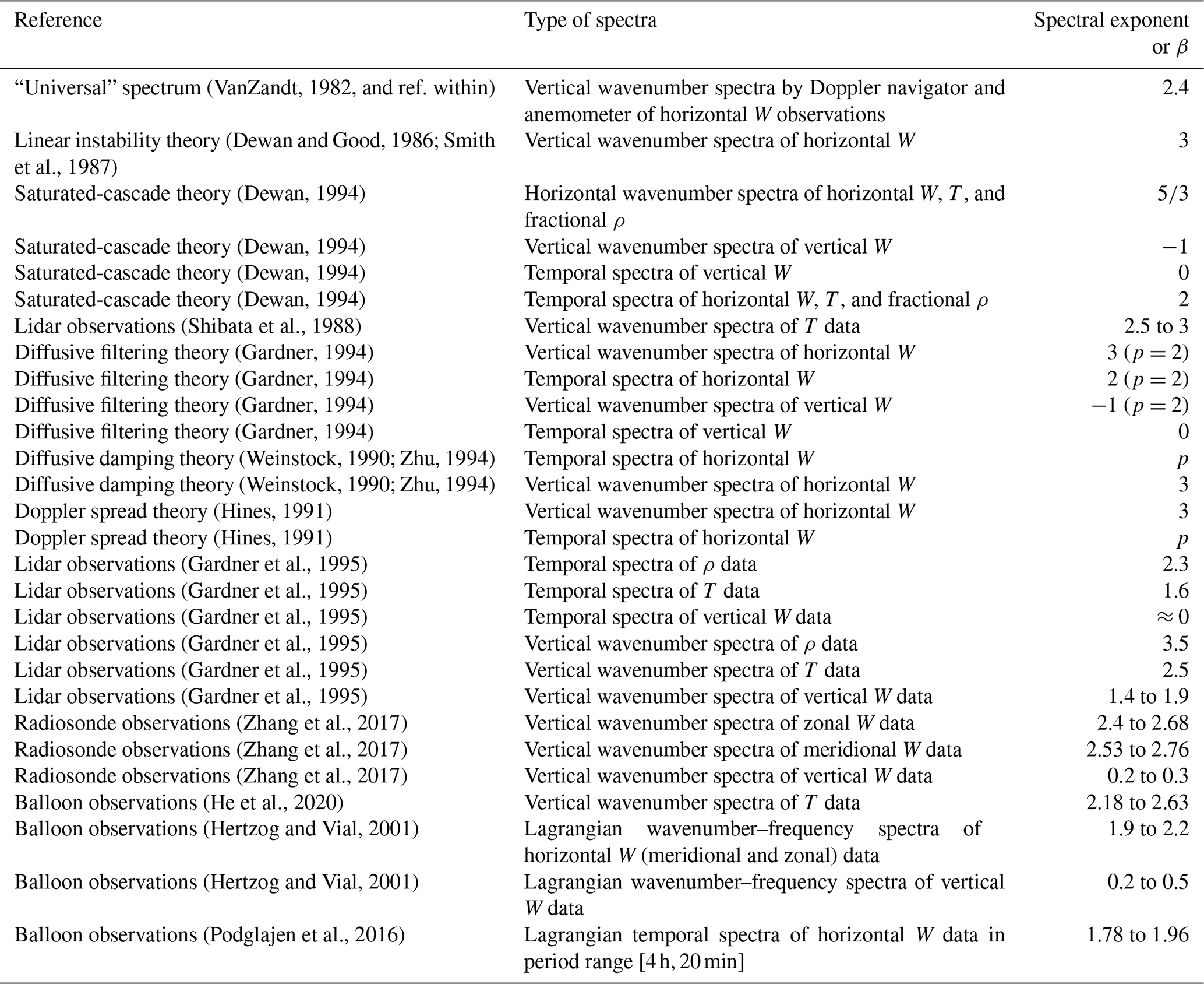
This GW spectrum exhibits a power law scaled by an exponent (or slope) β, which describes the rate at which wave energy changes with its wavenumber (or frequency). The basis for this spectrum for atmospheric GWs is supported not only by a strong foundation in theoretical works (Dewan and Good, 1986; Weinstock, 1990; Hines, 1991; Dewan, 1994; Gardner, 1994), but also in observational studies (Smith et al., 1987; Fritts et al., 1988; Gardner et al., 1995; Nastrom et al., 1997; Zhang et al., 2006, 2017). These values of β depend on not only the type of spectra (e.g. temporal or horizontal, or vertical wavenumber) but also the geophysical variables measured (e.g. temperature, horizontal or vertical wind); see Table A1 for a summary. Thus, an accurate estimation of β is essential to validate different theoretical predictions of GW power spectral densities (PSDs) (Dewan and Grossbard, 2000) and improve climate models and weather forecasts (Lindgren et al., 2020).

Determining β from empirical atmospheric measurements is challenging due to various factors, such as the inevitable presence of data gaps, observational noise, and the finiteness of data length and resolution. Data gaps can occur for numerous reasons, including instrumental errors, data transmission issues (e.g. due to weather conditions like clouds in the case of lidar), and signal interference (in the case of radar). When gaps exist in multiscale time series, data points representing certain frequencies are lost, which distorts the spectra and introduces significant bias into the estimation of β (Brown and Christensen-Dalsgaard, 1990; Rigling, 2012). To minimize the effect of these gaps on the spectra, data-filling schemes are often applied. Though linear interpolation is usually used to fill in these gaps (Meisel, 1978; Lepot et al., 2017), even adaptively implemented interpolators produce artefacts in the time series at low gap percentages (GPs), which contribute additional bias in the spectra (Schulz and Stattegger, 1997; Hall and Aso, 1999). Bias in spectral estimates can also be caused by other relevant sources, such as spectral leakage, steep spectra (β>2), and in-signal components with larger periods than the observed time span T (Klis, 1994).

In this paper, we systematically quantify the advantages and limitations of estimation methods of GW spectra in handling these error sources. We also propose a procedure for selecting unambiguously suitable methods for β estimation. Even though this study is motivated by the analysis of atmospheric GWs, the conclusions and the methods can be generalized to different fields with similar time-series characteristics in other branches of geophysics. Two commonly used methods are considered, namely the fast Fourier transform (FFT) (Cooley and Tukey, 1965) and the generalized Lomb–Scargle periodogram (GLS) (Zechmeister and Kürster, 2009), as well as the fairly recent Haar structure function (HSF) (Lovejoy and Schertzer, 2012). FFT is the standard method to analyse spectra of evenly sampled data. The Lomb–Scargle periodogram (LS) has been used in many studies as the main analysis method (or as a reference) of GW spectra (e.g. Hall and Aso, 1999; Zhang et al., 2006; Guharay and Sekar, 2011; Qing et al., 2014). As far as the authors are aware, HSF has never been used in atmospheric GW studies. Both GLS and HSF are specifically known to handle unevenly sampled data. In an effort to closely mimic real observations of GWs, we simulate time-series data with varied levels of complexity, beginning with a signal with one frequency and increasing in complexity to a superposition of sinusoids with randomly distributed frequencies (and phases).

Previous studies have investigated these spectral methods and others for estimating power-law spectra and compared their performance using synthetic and observed data. For instance, Zhan et al. (1996) found that using FFT of linearly interpolated signals is the best approach to analyse radar wind data at 50 % GP (only for the case of $\mathit{\beta }=\mathrm{5}/\mathrm{3}$) compared to the correlogram and LS. However, a quantitative analysis of the effect of changing β or the GP was not conducted. Similarly, Munteanu et al. (2016) showed that FFT outperforms LS, Z transform, and discrete Fourier transform in estimating β from Venus' magnetic field data, although the effect of changing β was not considered either, since the power-law spectra were not simulated. In contrast, Hébert et al. found that HSF consistently surpassed other methods in estimating β, without the need to interpolate the gapped (simulated palaeoclimate) data for $\mathit{\beta }\in (\mathrm{0},\mathrm{3})$, except in the case of $\mathit{\beta }\in (-\mathrm{1},\mathrm{0})$, where they concluded that LS would be the best option (Hébert et al., 2021). Nonetheless, the impact of altering the GP was not quantitatively presented; instead, the skewness of the gaps' (gamma) distribution was used as a parameter to refer to the irregularity of the time series. These three studies showed that the LS method suffers from significant leakage in the case of power-law spectra, which persists even when multi-taper methods (MTMs) are used.

The rest of the paper is organized as follows: in Sect. 2, we describe the methods used in our study, including a description of FFT, GLS, and HSF. In Sect. 3 we introduce the data simulation procedures. In Sect. 4 we discuss data processing. In Sect. 5 we present the results of our simulations, comparing the performance of these methods in different scenarios. In Sect. 6 we discuss the implications of our findings and provide recommendations for spectral analysis of GW time series with data gaps. Finally, in Sect. 7, we present a summary of our relevant results and conclusions.

2 Spectral methods

2.1 The fast Fourier transform

FFT is the most commonly used method for estimating frequency spectra of evenly sampled data (Cooley and Tukey, 1965). It enables the approximation of a time series sampled from a continuous distribution over discrete time steps, through a series of complex sine and cosine waves with varying frequencies. Under the assumption of a unit sample interval, (forward) FFT converts a time series z_n of length N from its original domain (time or space) into a set of coefficients Z_k in the (temporal or spatial) frequency domain by employing the following relation:

$$\begin{array}{}\text{(1)}& Z_k=\sum _{n=\mathrm{0}}^{N-\mathrm{1}}{z}_n{e}^{-\mathrm{2}\mathit{\pi }ikn/N},k=\mathrm{0},\mathrm{1},\mathrm{\dots },N-\mathrm{1}.\end{array}$$

In our work, FFT will serve as the benchmark spectral estimation method. The expected Fourier transform of a discretized signal is given by the convolution of the true transform and the transform of a Dirac comb window function designating those measurement times (Vanderplas, 2018). In the case of gapped data, the symmetry in the Dirac comb is destroyed, causing the resulting transform to be noisy with incorrect peak positions and heights. Consequently, the true transform of gapped data will not be recoverable. This disadvantage can be bypassed by applying data reconstruction methods such as interpolation, sparse approximation, etc., to approximate the true Fourier transform (Babu and Stoica, 2010). Unfortunately, these reconstruction methods can introduce artefacts into the signal, which depend on the distribution of the gaps and their sizes (Munteanu et al., 2016).

2.2 The generalized Lomb–Scargle periodogram

The GLS periodogram developed by Zechmeister and Kürster (2009) offers a method for estimation of the PSD of unevenly sampled time series. It is a generalization of Lomb's least-squares approach (Lomb, 1976), which is equivalent to the modified Schuster's periodogram (Schuster, 1898; Scargle, 1982) (based on FFT) in the case of evenly sampled data. GLS produces a spectrum by least-squares fitting a model of a weighted sinusoid given by

$$\begin{array}{}\text{(2)}& y\left(t\right)=a\cos \mathit{\omega }t+b\sin \mathit{\omega }t+c\end{array}$$

to the time series at each sampled frequency ω. The offset c compensates for the assumption that the mean of the time series $\stackrel{\mathrm{‾}}{z}$ is equal to the mean of the fit $\stackrel{\mathrm{‾}}{y}$. This floating-mean approach is advantageous, considering that the mean of a periodic signal may change statistically, especially for small N (Ferraz-Mello, 1981). Furthermore, the purpose of using weighted sums is to account for the observational noise for which the original LS does not.

The LS method has often been used to seek dominant periodic frequencies or cycles (Zhang et al., 1993; Pichon et al., 2015; Rao et al., 2017), analyse seasonal changes in significant modulations of GW fields (Beldon and Mitchell, 2010), and estimate the spectral indices β and amplitudes of GW power-law spectra (Hall and Aso, 1999; Zhang et al., 2006; Guharay and Sekar, 2011; Qing et al., 2014). In addition, LS is known as the most efficient method for estimating the variance in both gapped and non-gapped stationary time series with a single periodicity, without the need to fill in missing data (Marinna et al., 2019). In contrast, Vio et al. (2010) found that LS is reliable for analysing neither semi-periodic nor aperiodic signals with non-stationary noise or signals made of more than one wave, without additional steps.

2.3 The Haar structure function

HSF is a mathematical tool used in conducting scaling analysis of signals (Lovejoy and Schertzer, 2012), which is based on the Haar wavelet (Haar, 1910). It is a simple yet powerful method for decomposing a signal x(t) whose power spectral density exhibits a power law, i.e. PSD∝τ^H with a scaling (Hurst) exponent H, over a scale (lag) $\mathit{\tau }=\mathrm{1}/f$, into fluctuations $\mathrm{\Delta }x=x(t+\mathit{\tau })-x\left(t\right)$. The first-order Haar fluctuations ℋ_τ at a lag τ are defined by the following relation:

$$\begin{array}{}\text{(3)}& {\mathcal{H}}_{\mathit{\tau }}\left(x\right(t^{\prime }\left)\right)={\displaystyle \frac{\mathrm{2}}{\mathit{\tau }}}\left|\sum _{t+\frac{\mathit{\tau }}{\mathrm{2}}<t^{\prime }<t+\mathit{\tau }}x\left(t^{\prime }\right)-\sum _{t<t^{\prime }<t+\frac{\mathit{\tau }}{\mathrm{2}}}x\left(t^{\prime }\right)\right|.\end{array}$$

The qth-order structure function S_q(τ) is then obtained as an approximation by ensemble-averaging these fluctuations as follows:

$$\begin{array}{}\text{(4)}& S_{\mathcal{H},q}\left(\mathit{\tau }\right)=\langle {\mathcal{H}}_{\mathit{\tau }}\left(x\right(t\left)\right)\rangle \approx {\mathit{\tau }}^{qH-K\left(q\right)}.\end{array}$$

In the quasi-Gaussian case, the moment scaling function is K(q)≈0, so for the first-order structure function (q=1) only H determines the scaling of mean fluctuations.

A power spectrum which follows a power-law PSD∝τ^β is related to the Hurst exponent by $\mathit{\beta }=\mathrm{1}+qH-K\left(q\right)$; since the power spectral density is a second-order moment, we take q=2. Thus, under our quasi-Gaussian approximation, we re-scaled HSF to a comparable scale to the PSD using the following relation:

$$\begin{array}{}\text{(5a)}& {\displaystyle }& {\displaystyle }{S}_{\mathcal{H},q=\mathrm{1}}\propto {\mathit{\tau }}^H\approx {\mathit{\tau }}^{\frac{\mathit{\beta }-\mathrm{1}}{\mathrm{2}}},\text{(5b)}& {\displaystyle }& {\displaystyle }{S}_{\mathcal{H},q=\mathrm{1}}\cdot {\mathit{\tau }}^{\mathrm{1}/\mathrm{2}}\propto {\mathit{\tau }}^{\mathit{\beta }/\mathrm{2}},\text{(5c)}& {\displaystyle }& {\displaystyle }{S}_{\mathcal{H},q=\mathrm{1}}^{\mathrm{2}}\cdot \mathit{\tau }\propto {\mathit{\tau }}^{\mathit{\beta }}\propto \text{PSD}.\end{array}$$

Despite the term K(2) being fairly small, it is nontrivial in the non-Gaussian case and for higher moments q, and HSF allows for its calculation (Lovejoy and Schertzer, 2012), but this is beyond the scope of this paper. HSF is particularly suitable for estimating the scaling exponent of time series with $H\in (-\mathrm{1},\mathrm{1})$ or $\mathit{\beta }\in (-\mathrm{1},\mathrm{3})$. This range of β values covers the vast majority of atmospheric processes from weather (where τ<10 d and $\mathrm{1}<\mathit{\beta }<\mathrm{3}$) to macroweather (where $\mathrm{10}\mathrm{d}<\mathit{\tau }<\mathrm{10}$–30 years and $-\mathrm{1}<\mathit{\beta }<\mathrm{1}$) systems. HSF also possesses the advantage of handling unevenly sampled data, which is a consequence of the fact that it is computed by taking the mean of absolute fluctuations (Lovejoy, 2014). Nevertheless, HSF is not employed to estimate the frequency of a wave or its amplitude, since it only measures how much frequency components contribute to the total variance. The Python code implementation of HSF is readily accessible (Mossad, 2023) and was derived from the R code originally developed by Raphaël Hébert (Hébert, 2021).

3 Data simulation

In this section, we present the simulation procedures used to generate time series similar to actual GWs measurements. In measurements, GWs can exhibit various behaviours, ranging from superposed waves within wave packets with multiple frequencies, amplitudes, and phases to more coherent quasi-monochromatic waves (Maekawa et al., 1984; Eckermann and Hocking, 1989; Sica and Russell, 1999). In Sect. 3.1, we simulate signals with each having one frequency to mimic quasi-monochromatic waves, by which the goal is to accurately estimate the correct frequency and amplitude of each signal. In Sect. 3.2, however, we simulate time series composed of a superposition of waves with random frequencies and power-law amplitudes. The exponents/slopes β of their power-law spectra are used to assess the bias in the spectral-analysis methods. While our simulation adopts a simplified linear saturation theory approach through the superposition of sine waves (Dewan and Good, 1986; Smith et al., 1987), we acknowledge that other explanations for the spectral character of GWs exist, including “nonlinear damping” (Weinstock, 1982, 1990; Gardner, 1994), “Doppler spreading” (Hines, 1991), “saturated-cascade similitude” (Dewan, 1994), and high-Reynolds-number “stratified turbulence” (Pinel and Lovejoy, 2014); see Table A1 for more details.

By analysing both simulations, we can determine the accuracy of each of the methods at different levels of signal complexity and identify potential limitations and sources of error in the analysis of GWs spectra. Random gaps are then introduced to resemble observational gaps for both simulations. The units and values of the variables used in this simulation have been chosen to represent average values or ranges characteristic of typical GW time series.

3.1 Single-frequency signal simulation

Quasi-monochromatic GWs can be observed under specific conditions where a single frequency dominates other components (Muraoka et al., 1988; Swenson et al., 1999). This kind of GW can be approximated as an evenly sampled single sinusoid $x\left(t\right)=A\sin (\mathrm{2}\mathit{\pi }ft+\mathit{\phi })$, with a known frequency f, phase shift φ, and amplitude A, at time t. For both simulations, the time resolution Δt is 5 min with a total span of T=6 h, as this resolution and this duration align with the average values of lidar measurements commonly used in atmospheric studies (Gardner et al., 1995; Gerding et al., 2008). As a result, the number of points N in each signal is equal to $\frac{T}{\mathrm{\Delta }t}=\mathrm{72}$. Each simulated sinusoid has an amplitude of A=4 K and a randomly chosen frequency f from the set $\mathrm{1}/\mathit{\{}\mathrm{6},\mathrm{3},\mathrm{1.5},\mathrm{1},\mathrm{0.5},\mathrm{1}/\mathrm{3}\mathit{\}}$ [h⁻¹]. Changing the frequency serves as a test to examine whether the bias in the methods is frequency-dependent. The phase shift φ is also randomly chosen from a uniform distribution within the interval [0,2π].

The amplitude of the time series is equivalent to the estimated height of the main peak in the spectrum. It is computed from the FFT coefficients (Eq. 1) as $A_{\text{FFT}}={max}_k\left(\frac{\mathrm{2}\left|Z_k\right|}{N}\right)$ and from the GLS fit coefficients (Eq. 2) as $A_{\text{GLS}}={max}_k\left(\sqrt{a_k^{\mathrm{2}}+b_k^{\mathrm{2}}}\right)$. The frequency of that peak f_k corresponds to the estimated frequency of the signal. As a metric for the accuracy of estimation of the true values of frequencies and amplitudes, we used the relative bias given by

$$\begin{array}{}\text{(6)}& \text{relative bias}={\displaystyle \frac{\text{value estimated}-\text{value expected}}{\text{value expected}}}.\end{array}$$

Since real data are susceptible to observational noise, it is crucial to consider the case where white noise is added to the simulated signal as a random variable r(t) from a standard normal distribution. Here, the signal-to-noise ratio is defined by $\text{SNR}=A^{\mathrm{2}}/\mathrm{2}{\mathit{\sigma }}_r^{\mathrm{2}}$, where ${\mathit{\sigma }}_r^{\mathrm{2}}$ is the noise variance (Horne and Baliunas, 1986). To strike an appropriate balance between capturing meaningful noise characteristics and minimizing low SNR bias, an average SNR value of 8 is chosen for this simulation.

3.2 Spectral power-law simulation

As reported before (see Table A1), the spectra of GWs are characterized by a power law; i.e. $\text{PSD}\propto \mathrm{1}/f^{\mathit{\beta }}$ (in the case of spatial data, $\text{PSD}\propto \mathrm{1}/(k,l,m{)}^{\mathit{\beta }}$, where k, l, and m are horizontal and vertical wavenumbers). On that account, we are interested in estimating the value of β of simulated time series whose spectra would have $\mathit{\beta }\in \mathit{\{}-\mathrm{1},\mathrm{0},\mathrm{1},\mathrm{5}/\mathrm{3},\mathrm{2},\mathrm{2.5},\mathrm{3}\mathit{\}}$ and comparing it with the true value. The simulated evenly sampled time series x(t) consists of a sum of M sinusoids, each with frequency f_i and power-law amplitudes $A_i=f_i^{-\mathit{\beta }}$, as follows (Rice, 1944; Billah and Shinozuka, 1990; Kirchner, 2005):

$$\begin{array}{}\text{(7)}& \begin{array}{rl}x\left(t\right)& \sim \sum _i^M\sqrt{A_i}\sin (\mathrm{2}\mathit{\pi }{f}_{i}t+{\mathit{\phi }}_i)\\ & =\sum _i^M\left(f_i{)}^{-\mathit{\beta }/\mathrm{2}}\sin \right(\mathrm{2}\mathit{\pi }\left(f_i\right)t+{\mathit{\phi }}_i).\end{array}\end{array}$$

We used for our simulation M=35 for each time series. It is driven by the objective of reconciling the inclusion of a minimum of 20 waves based on observational (Sica and Russell, 1999) and modelling (Dewan, 1994; Hamilton, 1997) suggestions while simultaneously incorporating a sufficiently large number of waves to mitigate random spectral errors (Keisler and Rhyne, 1976; Shinozuka, 2005). This approach enables the demonstration of the power-law spectrum without the need for excessive averaging. The phase shifts φ_i are also randomly chosen from a uniform distribution within the interval [0,2π]. The frequencies f_i are statistically independent, uniformly distributed random values, selected within the range $\left[\frac{\mathrm{1}}{T},\frac{\mathrm{1}}{\mathrm{2}\mathrm{\Delta }t}\right]=\left[\frac{\mathrm{1}}{\mathrm{6}\mathrm{h}},\frac{\mathrm{1}}{\mathrm{10}\min }\right]$. Hence, the time series is composed of non-harmonic components and there are no favoured frequencies, which is a better approximation of atmospheric GWs than an idealistic case where frequencies are only integer multiples of a fundamental frequency. Here, x(t) is proportional to the square root of the amplitudes A_i, since β is estimated from PSD-normalized spectra, which are the squared modulus of the amplitudes.

The PSD is obtained by FFT using the relation $\frac{\mathrm{2}{Z}_k{Z}_k^{*}\mathrm{\Delta }t}{N}$, where $Z_k^{*}$ is the complex conjugate of Z_k. This definition is equivalent to the GLS spectrum $\frac{N\left|a_k^{\mathrm{2}}+b_k^{\mathrm{2}}\right|\mathrm{\Delta }t}{\mathrm{2}}$ of evenly sampled data. HSF is however normalized according to Eq. (5c) to estimate a comparable scale to the PSD. The bias in β estimation is defined for this simulation as

$$\begin{array}{}\text{(8)}& \mathit{\beta }\text{bias}=\text{value estimated}-\text{value expected}.\end{array}$$

3.3 Gap simulation

After creating a time series with the desired spectral properties, gaps are introduced by randomly removing data points (except both endpoints), assuming that all data points are equally likely to be removed (i.e. a uniform distribution). Based on the simulated GP p in the data, an integer number of random points $N_G=\frac{N\cdot p}{\mathrm{100}}$ is removed. Thus, a 0 % GP means that no points were removed, while a 50 % GP means that 36 points were randomly removed, since N=72. To assess the dependence of bias in spectral-analysis methods on the gaps, we conducted simulation runs spanning GPs ranging from 0 % to 90 % in increments of 10 % for each time series analysed. Each of these simulation runs was repeated 1000 times at each GP increment to ensure the statistical significance of our results, since the frequencies, phases, and gaps are randomized. Then we computed the average values of the estimated amplitude and period (for the single-frequency signal simulation) and β (for the spectral power-law simulation).

4 Processing steps

Before applying spectral methods to the generated time series from the simulations in Sect. 3, the following steps are taken:

• The time series is first interpolated using the original time step of 5 min; this is only necessary for FFT.

• The mean of the signal $\stackrel{\mathrm{‾}}{z}$ is subtracted to account for the zero-frequency component of the Fourier transform Z₀.

When computing the spectrum for a time step Δt, the frequency grids of all methods are defined as follows:

• The frequency range spans from $\frac{\mathrm{1}}{T}$ to $\frac{\mathrm{1}}{\mathrm{2}\mathrm{\Delta }t}$.

• The frequency spacing is given by $\mathrm{\Delta }f=\frac{\mathrm{1}}{T}$.

In the presence of gaps where Δt is not constant, the Nyquist frequency is then defined as follows:

• $f_{\text{Ny}}=\frac{\mathrm{1}}{\mathrm{2}p}$, where p is the largest value that allows $t_i=t_{\mathrm{0}}+n_{i}p$ to be possible for all t_i values, and n_i comprises integers (Eyer and Bartholdi, 1999). This value corresponds to the same Nyquist frequency as that of our non-gapped data, which is 0.1 min⁻¹.

• This approach is more appropriate for GLS and HSF than applying a “pseudo-Nyquist” limit based on an average or a minimum value of Δt (Scargle, 1982; Vanderplas, 2018).

To estimate β, the spectra are fitted by taking the following steps:

• A maximum likelihood estimator (MLE) is employed to determine the fit parameter β (Duvall and Harvey, 1986).

• The MLE fit involves minimizing the negative log-likelihood function −ln L(O) of observations O_i at frequency f_i using the equation

  $$\begin{array}{}\text{(9)}& -\ln L\left(O\right)=\sum _{i=\mathrm{1}}^n\ln \langle O_i\rangle +{\displaystyle \frac{O_i}{\langle O_i\rangle }},\end{array}$$

  where 〈O_i〉 refers to the power-law model $c\left(\frac{\mathrm{1}}{f^{\mathit{\beta }}}\right)$ being fitted, with c as a normalization coefficient.

• The MLE fit is recommended over least-squares regression because the latter assumes a Gaussian distribution of periodogram residuals, leading to a biased estimate of β (Clauset et al., 2009).

5 Results

5.1 Single-frequency signal

First, we show an example of the time series generated by the simulation described in Sect. 3.1, which consists of a 0.5 h wave in a 6 h time series. As can be seen in Fig. 1a, in the absence of gaps, an accurate estimation of the 4 K amplitude and the 0.5 h period of this signal is acquired by both GLS and FFT. In addition, the spectra obtained by FFT and GLS are (as expected) equivalent in the case of evenly sampled data (Scargle, 1982). When the random gaps replace 50 % of the data points, a significant difference between the amplitude spectra is observed; see Fig. 1b. Both methods still provide an accurate estimate of the signal's period. Linear interpolation of the 50 % gapped signal preserves the structure of the wave but loses some of the high-frequency components, which leads to a significant underestimation of the amplitude by 43 % in the FFT spectrum. In contrast, the amplitude of the highest peak in the GLS spectrum is not affected by the gaps and has not changed from the expected value.

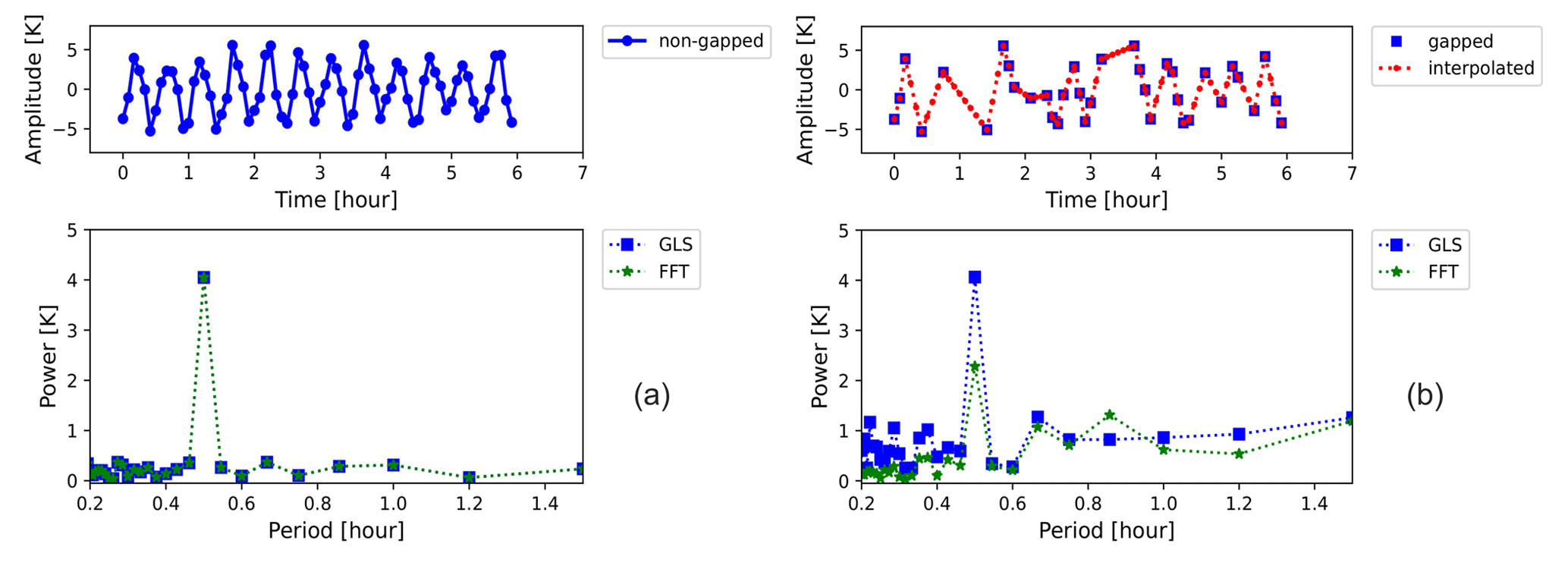
Figure 1 Time series of a 0.5 h wave in a 6 h observation time generated according to Sect. 3.1. Panel (a) shows the time series (upper left) and its temporal amplitude spectrum (lower left) in the absence of gaps. Panel (b) shows the time series (upper right) and its temporal amplitude spectrum (lower right) after the addition of a number of random gaps equal to 50 % of the total data length.

When comparing average relative period bias for different simulation periods, Fig. 2a shows that GLS demonstrates no period bias below 80 % GP and a negligible bias beyond (within ±20 % deviation interval). Figure 2b shows, contrarily, that the smaller the simulated period of the signal, the more FFT overestimates it at GPs larger than 40 %. This is due to linear interpolation replacing the removed high-frequency components with lower-frequency ones, which eventually dominate as the GP gradually increases. To put these results in perspective, at 70 % GP, FFT inaccurately determines the period of a 0.5 h wave as 2.93 h (i.e. overestimates it by 486 %). Given that there are quite few data points left in the time series at 70 % GP, it is expected that FFT is not able to recover the correct period; however, GLS is still capable of obtaining the exact value of the period (i.e. an error of 0 %). Not only is GLS a much better estimator of the period on average, but also since its standard deviation remains trivially small until 80 % GP, it is a more reliable choice on a case-by-case basis.

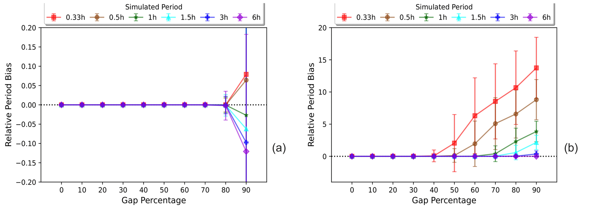
Figure 2 Comparison of relative period bias (Eq. 6) as a function of the gap percentage for GLS (a) and FFT (b), here shown for each simulated period (frequency). The bias is estimated from the average estimated values of the periods, and its standard deviation is scaled accordingly. Note that the y axis (relative period bias) is limited between $[-\mathrm{0.2},\mathrm{0.2}]$ for GLS and $[-\mathrm{4},\mathrm{20}]$ for FFT. This shows how extremely different the accuracy of each method is.

Similarly, FFT's amplitude bias experiences clear dependency on the frequency of the signal, while GLS demonstrates a negligible amplitude bias at GPs below 80 %; see Fig. 3. In particular, the results show that the mean estimated amplitude from the FFT spectrum deviates exponentially from the expected value as the frequency of the signal increases, even at gap percentages below 50 %. In addition, the standard deviation of amplitude estimation by GLS increases as the GP increases, although it remains within a ±10 % deviation interval up to 80 % GP. On the contrary, the standard deviation of amplitude estimation by FFT significantly increases as both the frequency of the signal and the GP increase, implying that FFT is more inconsistent and highly sensitive to missing data, especially for high-frequency signals.

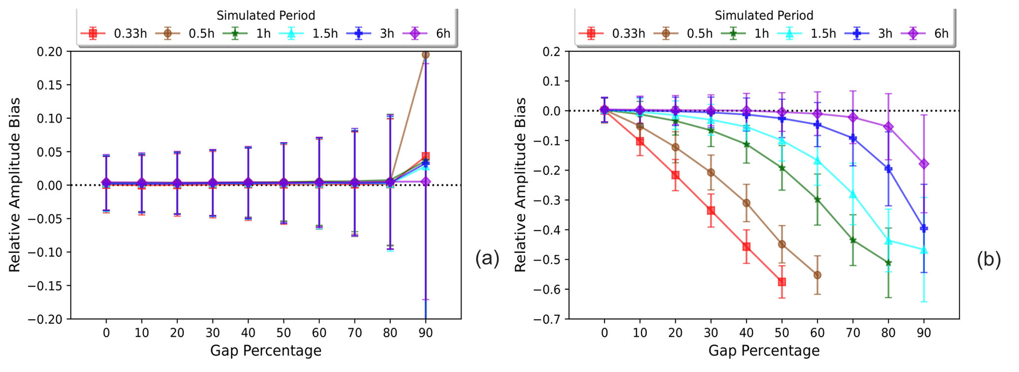
Figure 3 Comparison of relative amplitude bias (Eq. 6) as a function of the gap percentage for GLS (a) and FFT (b), here shown for each simulated period (frequency). According to Fig. 2b, past a certain GP threshold, the highest peak in the FFT spectrum does not belong to the true frequency but to meaningless interpolation noise. For this reason, the amplitude bias reported in Fig. 3 is limited by relative period bias<3, since amplitude values beyond this threshold should not be relied upon. Note that the upper and lower limits of the y axis are different for each method as well.

Overall, GLS provides a more robust estimation of the period and amplitude of gapped time series, while FFT's performance is simultaneously dependent on the GP and frequency of the signal.

5.2 Spectral power-law signal

A time-series example is shown in Fig. 4 to illustrate the complexity of a signal produced according to Sect. 3.2 for β=2, showcasing the signal before and after the introduction of gaps. As the percentage of gaps in the data increases, the impact on the spectral components varies depending on their frequency range. High-frequency components (rapid fluctuations over short periods) are most vulnerable when data are being removed. Subsequently, the lower-frequency components (slow variations over longer periods) follow, exhibiting greater resilience to data gaps. In essence, a considerably greater number of gaps are required to significantly affect the estimation of the latter. A distorted spectrum of this time series can be seen, which is a result of the limited sample length and resolution (Roberts et al., 1987). In addition, as the signal comprises numerous waves with random frequencies, the presence of closely spaced frequencies leads to the emergence of complex and broad peaks in the spectrum (Horne and Baliunas, 1986; Dewan and Grossbard, 2000).

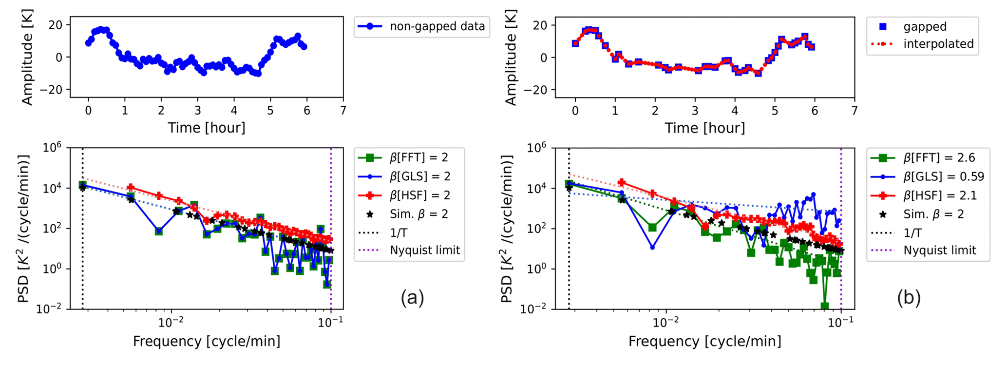
Figure 4 A time-series example (upper left and right) generated by the spectral power-law simulation (according to Sect. 3.2) with a spectral exponent of β=2 within a 6 h observation time, before (a) and after (b) the addition of 50 % gaps. The estimated power spectral densities of both non-gapped and gapped time series are shown in the lower left and right. Here, both x and y axes in the spectra figures were log-scaled so that a linear function can be identified. The dotted lines (in red, green, and blue) represent the fits of the PSD of each method.

In the absence of gaps, the true value of β is accurately estimated from the spectra of all methods (see Fig. 4a). However, after removing 50 % of the data points (Fig. 4b), the estimated spectrum by HSF remains relatively unaltered, while the GLS and FFT spectra diverge. The overestimation of β (bias=0.6) by FFT is due to the amplitudes of high-frequency components being underestimated, which is a result of the interpolation (Schulz and Stattegger, 1997; Hall and Aso, 1999). This overestimation of β can also be explained by the fact that these interpolated (high-frequency) components contribute locally by β=3 to the overall slope of the spectrum, which results in positive bias when the true β is less than 3 (Lovejoy, 2014). In the case of HSF, where no interpolation of the signal is done, an even smaller bias (0.1) results. In contrast, the true power law can be seen for the first few low frequencies in the GLS spectrum; then it starts to flatten at intermediate and high frequencies with a substantial bias of −1.41. This occurs because the lack of data points constrains the least-squares fit by GLS, which leads to the interpolation of power at these frequencies (i.e. a flat line).

For a statistically significant picture, we show the distributions of estimated β values from 1000 simulation runs in Fig. 5. In the non-gapped case (see Fig. 5a), the distributions of all methods overlap within a small standard-deviation range of ±0.2 around β=2. In contrast, we see that gaps cause the estimated β values from the FFT spectra to shift their distribution to higher values around β=2.3 in Fig. 5b, while the distribution of GLS becomes narrower and is diverted far below the expected value of 2. The mean of estimated β values from HSF spectra is clearly the closest to both the true value and its mean in the absence of gaps, which shows consistency and less sensitivity to the gaps. It is worth noting that the distributions in Fig. 5a show that even in the absence of gaps, estimated β lies mostly within the range of [1.5,2.5] and not exactly at 2, as single spectra are distorted without averaging. It is also important to mention that the results of the bias are almost identical whether β is estimated from averaging power-law exponents of single spectra or it is estimated from fitting an averaged spectrum.

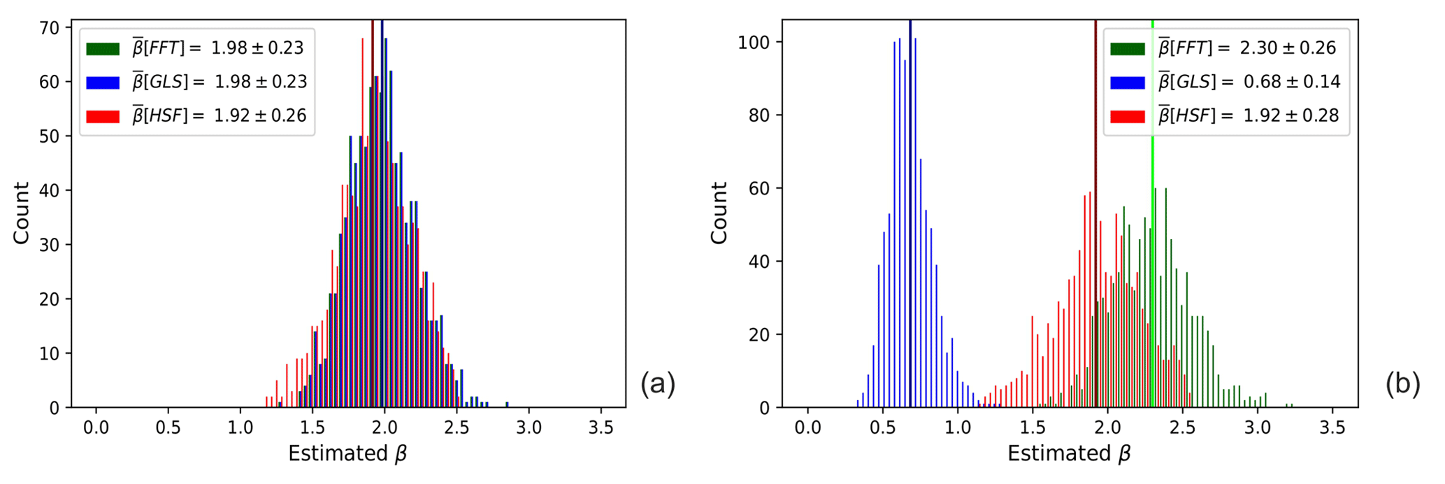
Figure 5 Histograms of the estimated β values from 1000 spectra of time series generated by the spectral power-law simulation (according to Sect. 3.2) before (a) and after (b) the addition of 50 % gaps. The simulated spectral exponent was β=2, and each time series had a 6 h observation span. The vertical lines in the histograms of the gapped case refer to the mean estimated values of β by each method.

To further explore the behaviour of the bias under different conditions, we evaluated the effect of changing the simulated value of β on the estimation bias (see Fig. 6). At 0 % GP, all methods show no bias, except for β>2 and $\mathit{\beta }=-\mathrm{1}$, where there is an apparent deviation. The first deviation is expected because the more β is larger than 2, the more the spectrum suffers from “low-frequency leakage” due to the finite length of the time series (Klis, 1994; Schulz and Mudelsee, 2002). The other case of small deviation takes place on the opposite end of the spectral slope range ($\mathit{\beta }=-\mathrm{1}$), where high frequencies dominate. The power at these frequencies is quite easily aliased, hence underestimated, as they are the closest to the Nyquist limit. These deviations do not mean that spectra of $\mathit{\beta }=-\mathrm{1}$ or β>2 cannot be obtained but that on average, they are very likely to be misestimated.

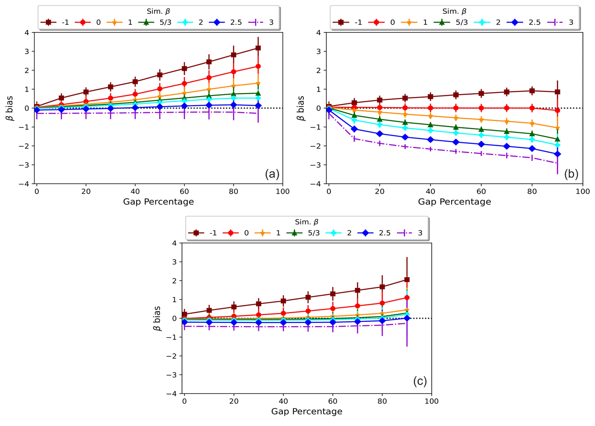
Figure 6 Comparison of the bias in the mean β estimates obtained from FFT (a), GLS (b), and HSF (c) as a function of the gap percentage. The results of each method are shown for spectra with power-law exponents $\mathit{\beta }\in \mathit{\{}-\mathrm{1},\mathrm{0},\mathrm{1},\mathrm{5}/\mathrm{3},\mathrm{2},\mathrm{2.5},\mathrm{3}\mathit{\}}$.

In the instance of gapped time series, our results show that as the GP increases, the biases in the estimated exponent also became more pronounced for all three methods. Similarly to the non-gapped situation, GLS demonstrates an exceptional efficiency in estimating flat spectra where β=0 with a negligible bias. This is a consequence of the absence of frequency dependency in a flat spectrum, which renders the gaps irrelevant in terms of introducing bias, since the GLS spectrum is already flat. As β increases (indicating a steeper decline in power with increasing frequency) and the percentage of gaps in the data increases, the bias in the GLS spectrum becomes more prominent. For instance, in the case of β transitioning from 1→3 where power is skewed towards low frequencies, gaps cause GLS to mistakenly assign excessive power at the missing high frequencies, ultimately resulting in a steady underestimation of β. In contrast, when $\mathit{\beta }=-\mathrm{1}$, high-frequency components dominate low-frequency ones. Consequently, there is a loss of power at these high frequencies as the gaps disrupt their sampling. This loss of power causes the GLS method to overestimate β, mirroring the GLS bias observed when β=1.

In similar fashion, both FFT and HSF demonstrate a relatively constant bias for β=3 of approximately −0.3 at all GPs. However, as β decreases from $\mathrm{2}\to -\mathrm{1}$, their biases monotonically increase as the GP increases. Nevertheless, HSF shows substantially less bias than FFT when the GP exceeds 10 %. The FFT bias is attributed to the established interpolation effects. Therefore, as more data points are interpolated, the FFT spectrum progressively underestimates the amplitude of the high frequencies. This underestimation results in the bias being positive for all β values, except β=3, where leakage causes FFT to overestimate these frequencies. Overall, averaging β values from single spectra is a good measure of the expected value because of their low standard deviation except at very high GPs.

In light of the aforementioned considerations, it can be argued that the FFT technique demonstrates competence in generating accurate spectral estimations for non-gapped time series. Nevertheless, it encounters challenges as the data incorporate an increasing number of gaps, necessitating interpolation techniques which introduce inherent biases. Meanwhile, HSF is demonstrated to be a particularly reliable approach for analysing GW time series with spectral power-law exponents $\mathit{\beta }\in \mathit{\{}\mathrm{1},\mathrm{5}/\mathrm{3},\mathrm{2},\mathrm{2.5},\mathrm{3}\mathit{\}}$ and in between. Its performance, however, exhibits limitations primarily in cases where the spectrum of a time series possesses a power-law exponent β<1. Notably, such occurrences have only been observed and predicted within measurements of vertical wind time series, as indicated in Table A1. One can reasonably anticipate that spectra falling within the range of β values between 1 and 3 will be prevalent across the majority of atmospheric time series.

Conversely, the GLS method yields similarly favourable outcomes, particularly for time series whose spectra are flat and high-frequency-dominated, so that it even surpasses the accuracy of HSF when β possesses values between −1 and 0. Nonetheless, the GLS method exhibits an increasing bias as the value of β increases beyond 0, rendering it a less certain choice for timescales extending beyond a few hours, which commonly occur in the context of atmospheric gravity waves. Clearly, the consistent and overall impeccable GLS performance in estimating periods and amplitudes of signals with single frequencies does not seem to translate to universally resolving the level of superposition of many random periodicities with power-law amplitudes.

6 Discussion

6.1 Low-frequency leakage

The problem of power leakage from low frequencies into higher ones arises as a result of the constrained frequency range, which itself is limited by the observed time span T. This leakage takes place not only in the case of spectra with β>2, but also in the spectra of time series with periods longer than T. GWs can often have these kinds of periods longer than the simulated time span of 6 h, and normally these periods are not resolved. Thus, we also quantitatively tested the effect of these long periods on the estimated spectra by adding three extra waves of 8, 10, and 12 h periods into the simulated time series. Two cases were examined, one where each of the three waves has an amplitude equivalent to the lowest-frequency component in each simulation. In another case, we scaled their amplitudes by the same power-law exponent β as all frequencies in the simulation.

In both cases, longer-than-T periods produced quite similar effects on the spectra, with a substantial positive bias observed for all signals with β<2 and a significant negative bias for β>2, even in the absence of gaps. For instance, Fig. 7a and b show an example of this leakage in averaged spectra for β=3, without and with the extra waves. A common feature of both cases is the spectral power being excessively concentrated at the lowest frequencies. When the extra long waves are added, the leakage becomes more drastic for GLS and FFT, and their absolute biases of β increase. In contrast, HSF is less affected by these long periods compared to FFT and GLS. This effect of longer-than-T waves in the time series resembles that of trends, which contribute to the spectral shape with a power-law exponent β=2 (Klis, 1994).

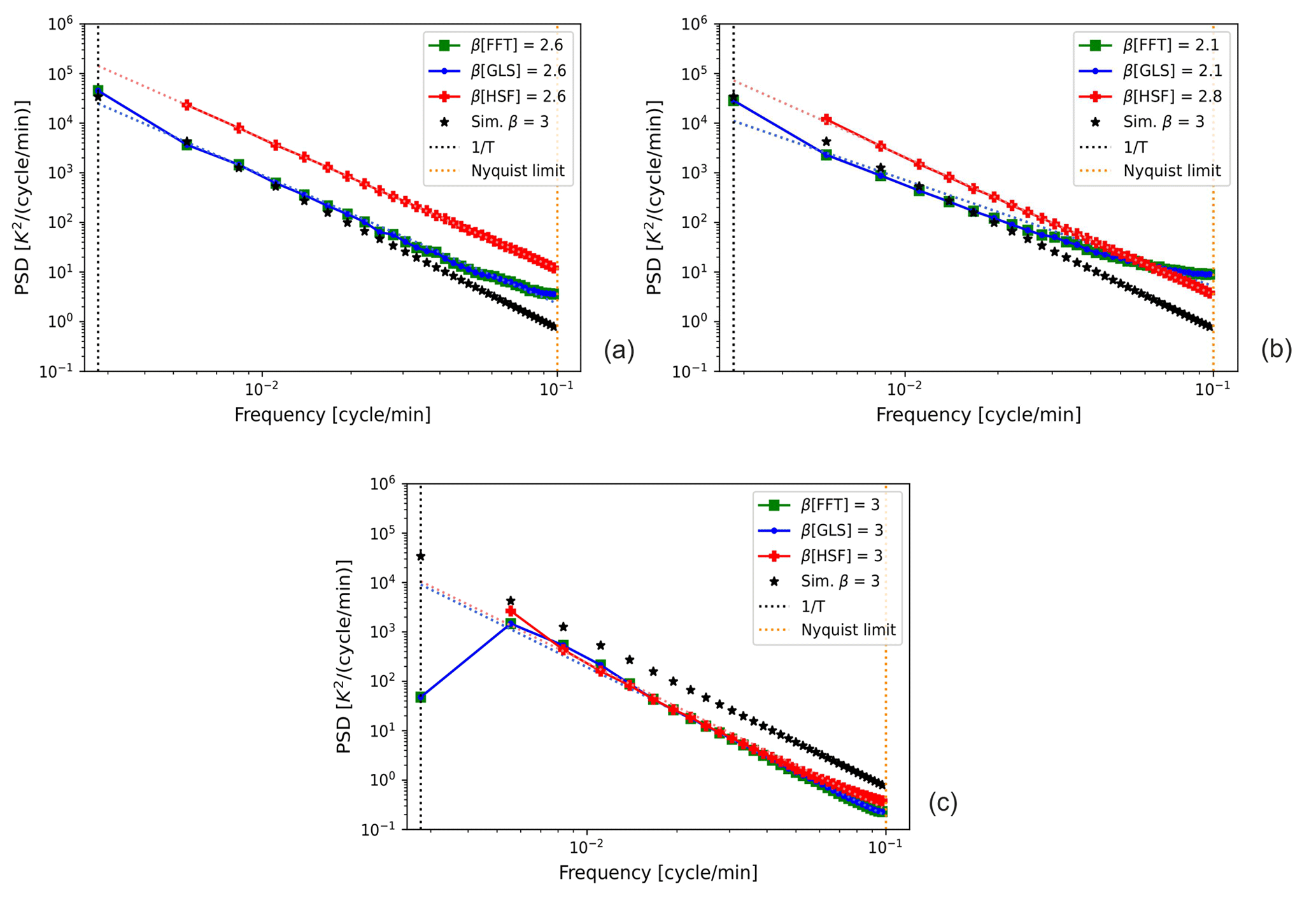
Figure 7 Averaged temporal spectra of non-gapped time series generated by the spectral power-law simulation with a spectral exponent of β=3 within a 6 h observation time: (a) non-prewhitened, without extra long waves; (b) non-prewhitened, after the addition of three extra waves with frequencies lower than $f=\mathrm{1}/T$ (particularly 8, 10, and 12 h) to the simulation; and (c) the postdarkened spectra of the prewhitened time series with extra waves. Here, both axes were also log-scaled so that a linear function can be identified. The dotted lines (in red, green, and blue) represent the fits of the PSD of each method.

While a weighted fit of the spectra can reduce the bias, it does not fully rectify the problem of leakage; it also requires a smoothed spectrum and may be confounded by other biases from observational noise, gaps, or method inefficiencies. One approach to counteract this leakage from unresolved low-frequency power is based on “prewhitening” the time series and then “postdarkening” the spectra (Blackman and Tukey, 1958). Prewhitening is a technique to decorrelate the time series (reduce its autocorrelation close to that of a white noise signal) before calculating the PSD (Keisler and Rhyne, 1976; Dewan and Grossbard, 2000; Guharay and Sekar, 2011). This step serves to decrease the rate of change in PSD(f) with frequency f; hence, the distribution of the power is more even. The prewhitened time series is obtained by the means of first differencing, where each data point is subtracted from its successive one; i.e. $\mathrm{\Delta }x\left(t\right)=x\left(t\right)-x(t-\mathrm{\Delta }t)$. By doing this, the contribution of the mean becomes negligible and trends are transformed into constants (Bieber et al., 1993). The spectrum of this prewhitened series Δx(t) is related to the original spectrum of x(t) by

$$\begin{array}{}\text{(10)}& {\text{PSD}}_{x\left(t\right)}\left(f\right)={\displaystyle \frac{{\text{PSD}}_{\mathrm{\Delta }x\left(t\right)}\left(f\right)}{\mathrm{2}(\mathrm{1}-\cos (\mathrm{2}\mathit{\pi }f\mathrm{\Delta }t\left)\right)}}.\end{array}$$

This factor 2(1−cos (2πf_nΔt)) is derived from the Fourier transform of the autocorrelation function of Δx(t) and is used to compensate for the prewhitening process (Houbolt et al., 1964). This compensation postdarkens (recolours) the resulting spectrum. Note that the spectrum of the prewhitened series Δx(t) should be smoothed first using a Hann window to suppress the random fluctuations before postdarkening.

In Fig. 7c, we present the postdarkened spectra after prewhitening the time series for β=3. This approach completely cancels out the bias in all methods for both cases. This confirms the effectiveness of the prewhitening and postdarkening method in correcting the leakage problem. However, this approach is not a perfect solution, since it may introduce additional bias for less steep spectra (where β<1) which do not suffer from leakage. When the spectrum is constant in the low-frequency part, the prewhitening process might cause it to be distorted as well.

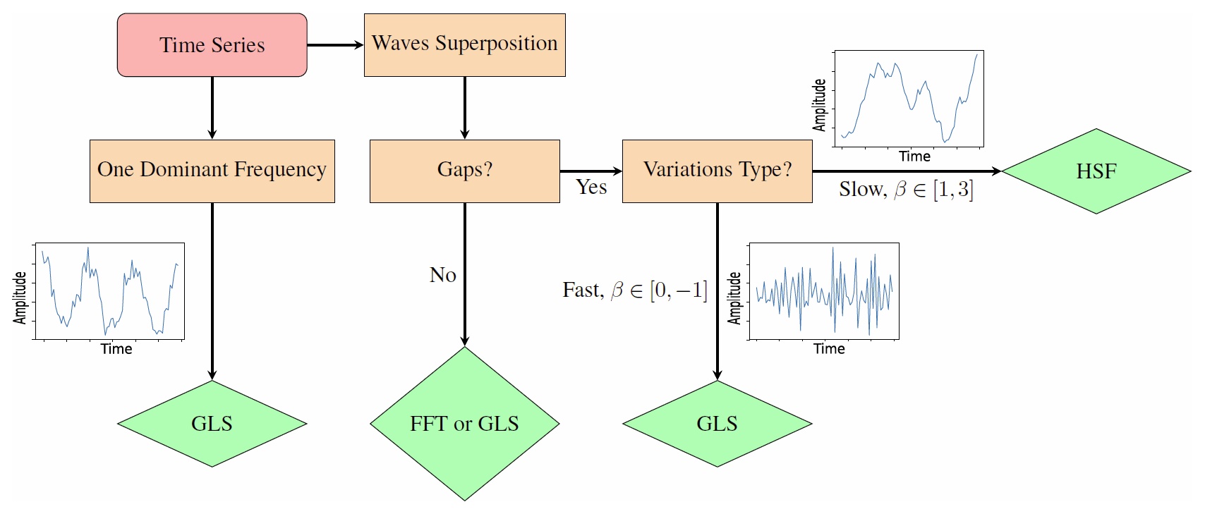
6.2 Method selection procedure

The spectral analysis of GW time-series data is a complex task that requires careful consideration of various factors. Based on our simulation results, we propose a flowchart (see Fig. 8) that outlines a practical guide for selecting appropriate spectral estimation methods for GW studies, taking into account the characteristics of the observed data such as their complexity and percentage of gaps in them. From the flowchart, it is clear that there are recognizable differences between the patterns of the time series of superposed waves and signals with one frequency. Even within the former classification, the anti-persistent time series whose spectra have $\mathit{\beta }\in [\mathrm{0},-\mathrm{1}]$ are still differentiable from those long-range-dependent ones where $\mathit{\beta }\in [\mathrm{1},\mathrm{3}]$. It is also safe to say that theoretical predictions of GW spectra with $\mathit{\beta }\in [\mathrm{0},-\mathrm{1}]$ exist only for measurements of vertical wind time series (see Table A1). Otherwise, $\mathit{\beta }\in [\mathrm{1},\mathrm{3}]$ spectra should be expected for the vast majority of atmospheric time series. Note that, even in the absence of gaps in the signal, caution must be taken if the estimated β is approximately equal to or less than 2. If it is, then it can be an accurate estimation or caused by one of the systematic errors such as interpolation or longer-than-T variations.

Figure 8 Recommended procedure for estimating power spectra of gravity wave time series.

7 Conclusions

The domain of observational analyses, especially in atmospheric physics, is vast and complex. The intrinsic nature of these measurements requires precision, reliability, and adaptability of analytical methods to extract meaningful insights. Observational gaps due to instrument failures or adverse conditions are also common in atmospheric physics. Our research on synthetic atmospheric gravity wave (GW) time series offers a comprehensive overview of different spectral estimation methods, shedding light on their strengths and limitations. The methods compared in this study are the fast Fourier transform (FFT) (which requires interpolation of gaps) and the generalized Lomb–Scargle method (GLS) and the Haar structure function (HSF) (both which can handle unevenly sampled data without interpolation). Their performance is assessed by evaluating whether the output spectra of simulated time series (with known a priori features and gap distributions) match the input parameters of the data, including the frequency, amplitude, and spectral slope. Building on our findings, we propose the following recommendations:

Determination of the time-series nature. Initially, the series is assessed to determine if it represents a pattern of a signal with one frequency. If it does, the analysis proceeds directly to using the GLS method, especially if the time series contains gaps and/or demonstrates rapid variations. Rather than interpolating these gaps to use FFT, which alters the data's characteristics, GLS offers far more accurate spectral estimates.

Evaluation of data gaps. For more complex series, particularly those characterized by a superposition of waves or the power-law spectrum, the data are first assessed for observational gaps. The presence of such gaps profoundly affects the accuracy of traditional spectral-analysis methods like FFT. If variations are rapid (i.e. the slope of that power-law spectrum β is in the range $[-\mathrm{1},\mathrm{0}]$), the series is again subjected to the GLS method. However, for slower variations such as the vast majority of atmospheric measurements, represented by a β value in the range of [1,3], the HSF method is consistently the least biased.

Mitigate low-frequency leakage. When the spectra of the time series with slow variations are analysed (even in the absence of gaps), it should be investigated whether low-frequency leakage takes place. Finite time series, very steep spectra, and waves with periods longer than the observed time span cause this kind of leakage. All tested methods, to varying extents, struggled with this leakage from unresolved low-frequency power, leading to biases in estimating the spectral slope β. Thus we recommend cautiously applying the approach of prewhitening the time series and postdarkening the spectrum to address this problem. Prewhitening can be actualized by first-differencing the series, which renders its spectrum close to that of white noise. Subsequently, postdarkening the spectrum is required to compensate for the prewhitening process via division by a frequency-dependent factor. Nevertheless, depending on the characteristics of the analysed time series, further steps (e.g. windowing) might be necessary to help counter other causes of leakage.

These sequential decisions highlight the importance of tailoring analysis methods to the characteristics of the data at hand. Employing a one-size-fits-all method can result in biased spectra, which are especially critical in GW parameterizations in all atmospheric models. Our recommendations, grounded in rigorous research on synthetic gravity wave time series, aim to guide researchers in making informed decisions, ensuring the accuracy of spectral results and advancing our understanding of the dynamics of the atmosphere.

Appendix A

(VanZandt, 1982, and ref. within)(Dewan and Good, 1986; Smith et al., 1987)(Dewan, 1994)(Dewan, 1994)(Dewan, 1994)(Dewan, 1994)(Shibata et al., 1988)(Gardner, 1994)(Gardner, 1994)(Gardner, 1994)(Gardner, 1994)(Weinstock, 1990; Zhu, 1994)(Weinstock, 1990; Zhu, 1994)(Hines, 1991)(Hines, 1991)(Gardner et al., 1995)(Gardner et al., 1995)(Gardner et al., 1995)(Gardner et al., 1995)(Gardner et al., 1995)(Gardner et al., 1995)(Zhang et al., 2017)(Zhang et al., 2017)(Zhang et al., 2017)(He et al., 2020)(Hertzog and Vial, 2001)(Hertzog and Vial, 2001)(Podglajen et al., 2016)

Table A1 Comparison of theoretical predictions and selected observed values of the power-law exponent β of GW spectra. Here T refers to temperature, W is wind, and ρ is density.