the Creative Commons Attribution 4.0 License.
the Creative Commons Attribution 4.0 License.
 | 31 Jan 2024
The EarthCARE mission: science data processing chain overview
Michael Eisinger
Fabien Marnas
Kotska Wallace
Takuji Kubota
Nobuhiro Tomiyama
Yuichi Ohno
Toshiyuki Tanaka
Eichi Tomita
Tobias Wehr
Dirk Bernaerts
The Earth Cloud Aerosol and Radiation Explorer (EarthCARE) is a satellite mission implemented by the European Space Agency (ESA) in cooperation with the Japan Aerospace Exploration Agency (JAXA) to measure vertical profiles of aerosols, clouds, and precipitation properties together with radiative fluxes and derived heating rates. The data will be used in particular to evaluate the representation of clouds, aerosols, precipitation, and associated radiative fluxes in weather forecasting and climate models.
The satellite embarks four instruments: the ATmospheric LIDar (ATLID), the Cloud Profiling Radar (CPR), the Multi-Spectral Imager (MSI), and the Broadband Radiometer (BBR). The science data acquired by the four satellite instruments are processed on ground. Calibrated instrument data – level 1 data products – and retrieved geophysical data products – level 2 data products – are produced in the ESA and JAXA ground segments. This paper provides an overview of the data processing chains of ESA and JAXA and explains the instrument level 1 data products and main aspects of the calibration algorithms. Furthermore, an overview of the level 2 data products, with references to the respective dedicated papers, is provided.
- Article
(2074 KB) - Full-text XML
- BibTeX
- EndNote


The Intergovernmental Panel on Climate Change (IPCC, 2023) has recognised the following:
While major advances in the understanding of cloud processes have increased the level of confidence and decreased the uncertainty range for the cloud feedback by about 50 % compared to AR5, clouds remain the largest contribution to overall uncertainty in climate feedbacks (high confidence).
The Earth Cloud Aerosol and Radiation Explorer (EarthCARE) mission will allow scientists to address this uncertainty, enabling a direct verification of the impact of clouds and aerosols on atmospheric heating rates and radiative fluxes. The collection of global cloud, aerosol, and precipitation profiles, along with co-located radiative flux measurements, will be used to evaluate their representation in weather forecast and climate models, with the objective to improve parameterisation schemes. EarthCARE is an ESA Earth Explorer mission that is being carried out in a collaboration with JAXA, which is providing one of the instruments. A mission overview by Wehr et al. (2023) describes the mission, its science objectives, observational requirements, and ground and space segments, including the instruments. EarthCARE will fly in a sun-synchronous, low-Earth orbit, with a mean local solar time of 14:00 ±5 min and a 25 d repeat cycle. It will fly at a rather low altitude (around 400 km) in order to maximise performance of the active instruments with respect their power needs. The satellite embarks four instruments: the ATmospheric LIDar (ATLID), the Cloud Profiling Radar (CPR), the Multi-Spectral Imager (MSI), and the Broadband Radiometer (BBR). The UV lidar, equipped with a high-spectral-resolution receiver and depolarisation measurement channel, will measure vertical profiles of aerosols and thin clouds and allow for classification of aerosol types. The highly sensitive 94 GHz (W-band) cloud radar will provide measurements of clouds and precipitation. Its sensitivity partly overlaps with the lidar, but its signal can penetrate through, or deep into, the cloud, beyond where the lidar signal attenuates. Furthermore, it has Doppler capability, allowing measurement of the vertical velocity of cloud particles. The imager has four solar and three thermal channels that will provide across-track swath information on clouds and aerosols and facilitate construction of 3-dimensional (3D) cloud–aerosol–precipitation scenes for radiative transfer calculations. The Broadband Radiometer measures solar and thermal radiances in three fixed viewing directions, along the flight track, which will be used to derive top-of-atmosphere flux estimates. ATLID and CPR data will be used to calculate atmospheric heating rates and radiative fluxes, using 1-dimensional (1D) and 3D radiative transfer models, the results of which can be compared against the flux estimated from EarthCARE Broadband Radiometer measurements.
Science data acquired by the instruments will be processed in ground segments in Europe and Japan. For an overview of the ESA and JAXA ground segments, including data dissemination, product latency (timeliness), and product levels, refer to Sect. 8.1 and 8.2 in Wehr et al. (2023). The two ground segments produce four level 1 instrument data streams containing calibrated and geolocated instrument measurements and a large number of geophysical data products (level 2 products).
These will take advantage of the synchronous data from multiple instruments, as well as use a dedicated, auxiliary stream of meteorological data provided by the European Centre for Medium-Range Weather Forecasts (ECMWF). The data products cover, for example, target classifications, vertical profiles of microphysical properties of ice, mixed and liquid clouds, particle fall speed, precipitation parameters, and aerosol types. This paper gives an overview of the processing chain development; the scientific data products; and their retrieval algorithms, simulation, and testing. Section 2 provides an overview of the processing chains at ESA and JAXA, which are defined in production models. The product naming and format are explained as well. Section 3 is dedicated to the level 1 data processors and products for the four EarthCARE instruments. Section 4 describes the auxiliary data processors and products, which make use of meteorological data from ECMWF and provide a common spatial grid for synergistic processors. Section 5 describes the level 2 processors and products, developed in Europe, Japan and Canada. Section 6 gives an overview of the development that has been undertaken for the processing chain, end-to-end simulator (E3SIM), generation and use of test data sets, and some of the lessons that have been learnt.
2.1 Overview
Instrument data are transmitted in Instrument Source Packets (ISPs), from the satellite to ground, via the satellite's X-band antenna, and enter the ESA Payload Data Ground Segment (PDGS). PDGS initial processing takes ISPs and puts them into a consecutive time sequence in an individual level 0 product for each of the four instruments, annotated with ancillary data. The instrument level 1 processors (Sect. 3), also called EarthCARE Ground Processors (ECGPs), take as their input these level 0 products and create level 1b products that are fully calibrated and geolocated instrument science measurements on the native instrument grid for CPR, ATLID, MSI, and the BBR single-pixel product. The nominal BBR product is integrated 10 km along track. Additionally, an MSI level 1c product is produced, with interpolation to a spatial grid common to all MSI bands.
ATLID, MSI, and BBR level 1 products are generated at the ESA PDGS and then shared with the JAXA ground segment. The CPR level 0 product is sent by the ESA PDGS to the JAXA ground segment, where it is processed into the CPR level 1 product, which is then shared with the ESA PDGS. This means that at the end of the level 1 processing step, level 1 products for the four instruments are available at both ground segments, as inputs to the two level 2 processing chains at ESA and JAXA (Sect. 5). These chains are almost independent, with the exception that ESA provides the BBR level 2b products for use at the end of the JAXA processing chain. Level 2 products are shared between agencies as well, which means all EarthCARE data products will be disseminated to users by both agencies, independent of where they were produced.
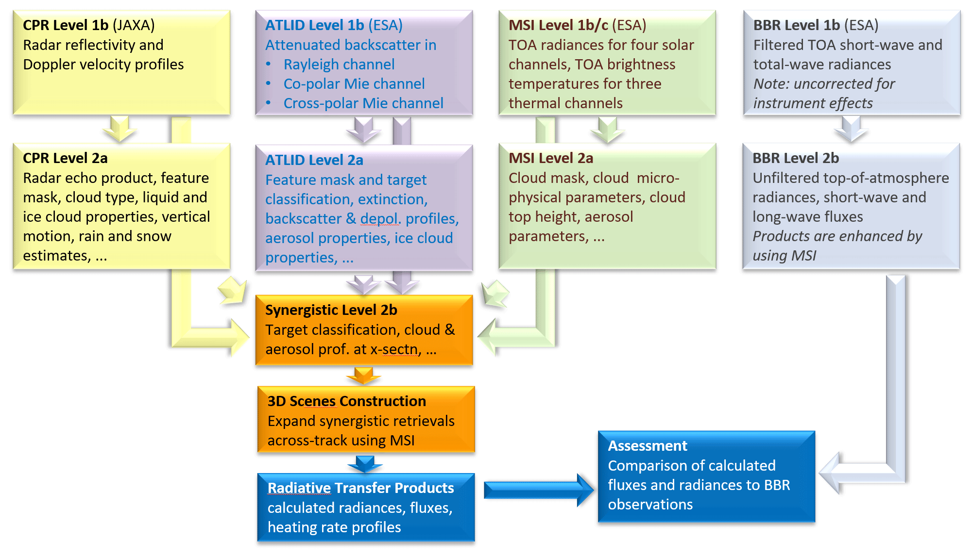
Figure 1Schematic overview of the EarthCARE processing chain. Level 1 processing is shared between ESA and JAXA according to their instrument responsibilities: ATLID, BBR, and MSI level 1 at ESA and CPR level 1 at JAXA. ESA and JAXA run their level 2 processing chains independently.
Figure 1 outlines the overall processing flow from level 1, via the single-instrument level 2a products to the level 2b products, combining measurements from two or more instruments. The main parameters at each processing step are indicated. Cloud and aerosol parameters are derived combining measurements from ATLID, MSI, and BBR and then used as input to radiative transfer models to derive top-of-atmosphere radiances and fluxes which are – at the end of the processing chain – compared to the radiances and fluxes derived from BBR measurements; see Wehr et al. (2023) (Sect. 5.4) and Barker et al. (2024).
Additionally, there are two auxiliary products (Sect. 4). These are ECMWF meteorological fields limited to the EarthCARE swath and a spatial grid shared by all instruments (“Joint Standard Grid”). These products are generated by the PDGS and shared with JAXA. They are used in both ESA and JAXA processing chains.
2.2 Product conventions and format
2.2.1 Product conventions
For ESA products and processors, each data product name and each processor name consist of two parts, connected by a hyphen: up to four letters XXXX, indicating the instrument, and up to three letters YYY, indicating the product content, XXXX-YYY. For most products, XXXX refers to one or more of the four EarthCARE instruments (A for ATLID, C for CPR, M for MSI, B for BBR). For example, the level 2a product A-FM refers to the feature mask (FM) derived from ATLID (A). The level 2b product AC-TC is the target classification (TC) derived from ATLID (A) and CPR (C). Auxiliary data products X-MET and X-JSG (Sect. 4) do not use any instrument measurements, so they use X instead of an instrument identifier.
JAXA data products are referenced by their product identifiers that are composed of two parts, separated by an underscore (e.g. CPR_CLP). The first two or three letters indicate the instruments used in the product (CPR = CPR, ATL = ATLID, MSI = MSI, AC = ATLID-CPR, ACM = ATLID-CPR-MSI, AM = ATLID-MSI, ALL = four sensors), and the latter three letters indicate the geophysical content of the product (e.g. CLP for cloud properties and RAD for radiation).
Parameters and dimensions within the data products follow a common set of conventions, which aim to harmonise naming across products and to make the names as self-explanatory and descriptive as possible. This means they can be rather long, as acronyms (apart from the instrument names) are avoided. The maximum length of a parameter name has been set to 63 characters. Other conventions concern the use of units and of certain standard suffixes, such as “flag” for a parameter that can only assume the values 0 and 1.
2.2.2 Product format
EarthCARE level 1 and level 2 data products will be provided as NetCDF-4/HDF5 files. This format has been selected as it is widely used in the community and is self-describing. Furthermore, a large number of software tools and libraries are available to read this format. Products use internal data compression, and each product covers one frame ( orbit or about 5000 km along track).
2.3 ESA processing chain
The complete set of ESA data products, and JAXA's CPR level 1b product, is generated according to the ESA EarthCARE Production Model, depicted in Fig. 2. The overall processing logic outlined in Fig. 1 can still be recognised in this detailed diagram. It includes level 0, level 1 and level 2 data products, as well as auxiliary and supporting data products. The processing chain is run at the PDGS, with two exceptions: the CPR level 1b product (Sect. 3.2) is generated in the JAXA ground segment using a data processor developed by JAXA, and the X-MET data product (Sect. 4.1) is produced at ECMWF using a data processor developed by ESA.
Every data product is produced by a processor. A processor is executable code implementing an algorithm which produces one or more data products. If a processor produces only one data product, the name of the processor and the name of the data product are the same. For example, the C-CLD processor produces only the C-CLD data product, and the A-FM processor produces only the A-FM data product. If a processor produces more than one data product, then it has a name different from the products. For example, the A-PRO processor produces the data products A-AER, A-ICE, A-TC, and A-EBD. Figure 2 gives an overview of all ESA processors and data products. Their interdependencies are shown as arrows, except for meteorological fields X-MET and Joint Standard Grid X-JSG where symbols – cloud and grid symbols, respectively – indicate their use in a data processor. If several data products are produced by one processor, this is indicated by a solid line around the respective data products, with the name of the processor given, for example, C-PRO and A-PRO. If a processor produces only one data product, the processor name is not explicitly indicated in the production model, as it is the same as the data product's name. For the data product user, the name of the processor is, however, not relevant. All data products can be fully identified by their data product name only.
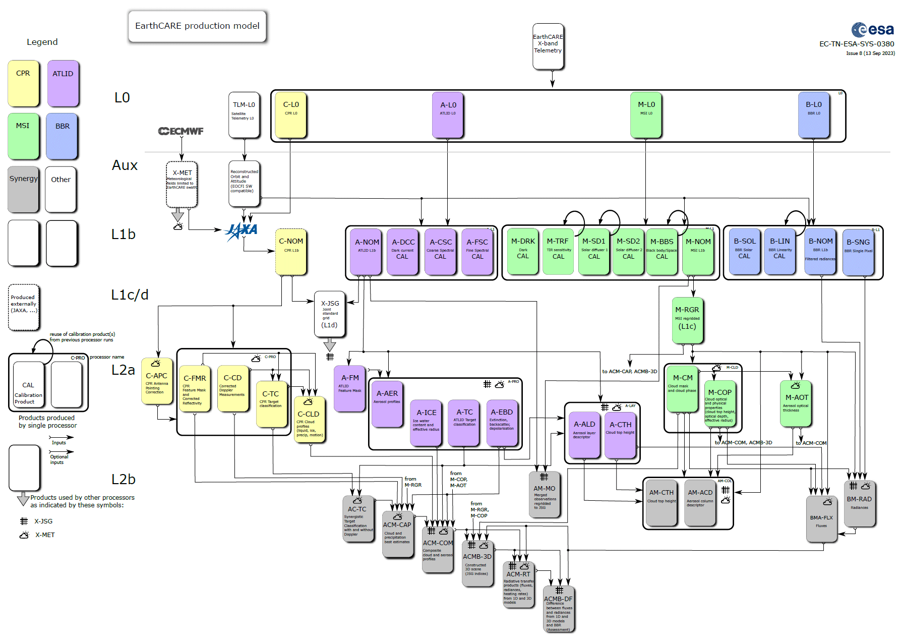
Figure 2The ESA EarthCARE Production Model (version 8, 13 September 2023) shows all ESA data products and the CPR level 1b product (C-NOM), which is produced by JAXA. Level 1 products (L1b, L1c/d) and auxiliary (Aux) products are described in Sects. 3 and 4. Level 2 products (L2a, L2b) and their retrieval algorithms are described in this AMT special issue according to Table 1 (L2a) and Table 3 (L2b).
The PDGS performs an instrument data calibration and monitoring function at the Instrument Calibration and Monitoring Facility (ICMF). Data, generally at level 1, from routine on-orbit calibrations of the three European instruments are plotted and reviewed at pre-specified intervals, in order to assess whether it is necessary to, for instance, modify a parameter – or a set of parameters – in the Calibration and Characterisation Database (CCDB) or perform an additional calibration. During the mission's operating phase (phase E2), data quality will also be monitored by a team, called the EarthCARE Data Innovation and Science Cluster (DISC), with members from ESA and the science user community, that assesses the geophysical data products. The PDGS is also responsible for mission planning, including for instrument calibration activities.
2.4 JAXA processing chain
The Production Model for JAXA products is illustrated in Fig. 3, showing the flow of the processors/algorithms from level 1 to level 2 products. Level 2 (L2) is categorised into level 2a and level 2b with the same definition as ESA products; level 2a products are those retrieved from a single instrument, while level 2b products are those derived from multiple instruments.
JAXA data products are categorised into two groups: Standard Products and Research Products. All products fall into one of the two categories, depending on the maturity of their algorithm development. Standard Products (Research Products) are indicated in solid-line (dashed-line) boxes in Fig. 3, respectively. JAXA data products are classified as Standard Products or Research Products.
-
JAXA Standard Products have the following characteristics:
-
Algorithms are relatively mature and have heritage from past studies.
-
They are strongly promoted to be developed and released.
-
They are processed in the JAXA Mission Operation System and released from the JAXA G-Portal website (https://www.gportal.jaxa.jp, last access: 22 January 2024), together with the standard products of other JAXA Earth observation satellite missions.
-
-
JAXA Research Products have the following characteristics:
-
Algorithms are new research developments that are challenging, yet scientifically valuable.
-
They are promoted to be developed and released.
-
They are processed and released from the JAXA Earth Observation Research Center (https://www.eorc.jaxa.jp/EARTHCARE/index.html, last access: 22 January 2024) and/or Japanese institutes/universities.
-
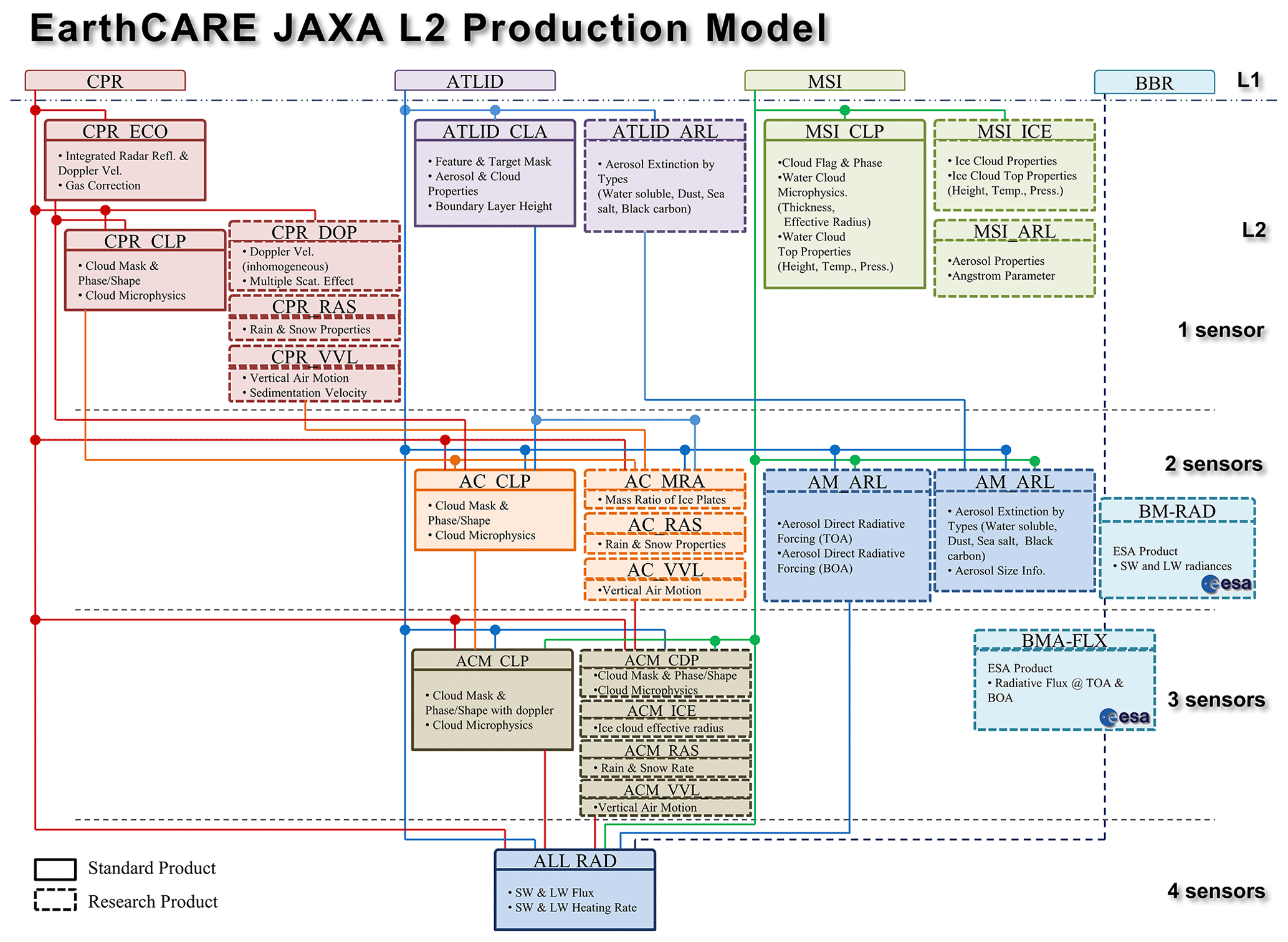
There are two categories of EarthCARE level 1 data products: nominal products, which contain calibrated instrument signals and are widely disseminated, and calibration products, which are used to optimise instrument settings, to monitor instrument performance, and to update calibration coefficients as needed. All this contributes to the calibration of the nominal products, which are fully calibrated, self-standing products. Calibration products are only disseminated to selected expert users.
This section, together with Sect. 5 of the companion paper by Wehr et al. (2023), provides the primary source of information on level 1 processing and calibration algorithms for EarthCARE.
3.1 ATLID
The high-spectral-resolution lidar, ATLID, will measure vertically resolved profiles of atmospheric and ground-backscattered optical power in three instrument channels.
-
Mie co-polar channel. The backscattered signal, co-polarised with respect to laser transmission, is received within the transmission bandwidth of the high-spectral-resolution etalon. Most of the backscatter from particles ends up in this channel, due to their narrow spectral broadening (small Doppler effect due to their slow movement).
-
Rayleigh co-polar channel. The backscattered signal, co-polarised with respect to laser transmission, is reflected by the high-spectral-resolution etalon. Most of the backscatter from molecules ends up in this channel, due to wider spectral broadening of the Rayleigh lines (large Doppler effect due to their fast movement).
-
Cross-polar channel. The total backscattered signal (Mie + Rayleigh) is cross-polarised with respect to laser transmission.
In order to increase the signal-to-noise ratio, it is possible to integrate two (or more) consecutive laser shots on board the ATLID instrument.
The ISPs generated by ATLID contain the measurement data as well as ancillary data such as the number of accumulated laser shots, instrument mode, time information, laser frequency, laser energy, detector saturation, and efficiency of the co-alignment loop. ISPs are transmitted from the satellite to the PDGS, where the level 0 data product is generated.
At level 0, the signal in each channel is a combination of each component of the atmospheric signals via several crosstalk effects:
-
Mie spectral crosstalk χ, the pollution of the Rayleigh channel by the Mie channel;
-
Rayleigh spectral crosstalk ϵ, the pollution of the Mie channel by the Rayleigh channel; and
-
polarisation crosstalk ψ∥ and ψ⟂, respectively, the pollution of the cross-polar channel by the co-polar channels and the co-polar channel by the cross-polar channels.
The ATLID level 0 products are ingested by the ATLID ECGPs which will process them and output the nominal as well as the calibration level 1 products. The nominal output products contain the range-corrected attenuated backscatter profiles.
The main step of the ECGP processing is to correct the acquired instrumental signals from this crosstalk effect, as well as to correct for the radiometric sensitivity of each channel, to retrieve range-corrected attenuated backscatter. This can be expressed with the following equation:
where N…(z) denotes the instrument signals per channel after radiometric pre-calibration, M is the 3×3 matrix of crosstalk correction coefficients, K is the diagonal 3×3 matrix containing the lidar constants for each channel, R(z) is the range for each altitude z, and is the range-corrected attenuated backscatter.
The level 1 processor uses instrument calibration data and algorithm settings from the CCDB. The CCDB is initially populated with data from ATLID on-ground characterisation and calibration. During flight it will be modified when necessary, updating some parameters on the basis of on-orbit calibrations. The frequency of a parameter update extends from almost-fixed – for a number of on-ground characterised parameters – to regularly updated – for the outputs of the in-flight calibrations.
The ATLID modes of operation supported by the ECGPs consist of the nominal lidar measurements interspersed with different calibration operations:
-
FSC (fine spectral calibration) consists of a fine frequency tuning of the laser around the current operational laser frequency, in order to minimise the spectral crosstalk on the Rayleigh channel. The optimal frequency is then selected for nominal measurements, performed once a week.
-
DCC (dark current calibration) consists of measuring the frequency-resolved dark current on each channel, by measuring the detector signals while the laser emitter is shut off, performed once a month.
-
CSC (coarse spectral calibration) consists of tuning the frequency of the laser emitter by relatively large frequency increments, in order to minimise the spectral crosstalk on the Rayleigh channel. A set of four to five optimal frequencies are chosen. The choice of the frequency is then done offline with respect to other instrumental criteria, performed at the beginning of life and if needed, for instance, due to a change of the instrument redundancy chain.
The frequency of calibration operations is indicative only and might have to be adjusted after launch, depending on instrument stability.
The complete list of ATLID level 1b products is now detailed.
-
A-NOM. The nominal ATLID level 1b data products contain geolocated, calibrated, range-corrected attenuated backscatter signal profiles, along with associated errors and with intermediate products from the processing: raw signals, signals after offset removal, signals after background removal, energy-normalised signals, and relative signals after crosstalk correction.
-
A-FSC. The fine-spectral-calibration products contain the optimal frequency and associated crosstalk, as well as quality criteria and intermediate products: geolocation of the samples, raw signals, and retrieved spectral crosstalk for each frequency setting.
-
A-DCC. The dark-current-calibration products contain dark-signal non-uniformity maps for the three channels and associated errors and quality criteria, as well as intermediate products: geolocation of the samples, raw signals, and offset as a function of the vertical sample for each channel.
-
A-CSC. The coarse-spectral-calibration products contain the frequency of each selected point in the optimal range (four to five in total), associated crosstalk, and intermediate products: geolocation of the samples, raw signals, and retrieved spectral crosstalk for each frequency setting.
The following sections describe the processing sequence.
3.1.1 Identification and counting of measurement data packets
Using flags raised by the ATLID instrument, the level 1 processor identifies the packets that contain invalid raw data. The packets are accepted with respect to several criteria: instrument mode, emitted beam quality (spectral emission quality), laser beam steering control loop status (indicating co-alignment between emitter and receiver), and detection health (background and signal saturation).
3.1.2 Geolocation
- 1.
Range evaluation location. Range information gives the distance from the receiver for each echo sample. Range computations are independent of instrument mode and do not use the measurement data stream; they rely only on the integration time and accumulation factor for the high-resolution (altitude 0 to 20 km) and low-resolution (altitude 20 to 40 km) part of the echo signal and the computer clock.
- 2.
Sample geolocation. Satellite position, altitude, and pointing data allow geolocation of atmospheric echoes to be performed. Satellite attitude and orbital information as a function of time, as well as instrument pointing (line of sight) information, is provided in input files to the software that will compute the following steps for each profile time stamp:
-
determination of position and attitude from the time stamp,
-
computation of line-of-sight targets,
-
computation of geodetic coordinates of samples.
-
- 3.
Calculation of atmospheric parameters associated with the samples. The geolocation information, atmospheric temperature, and pressure are attributed to each sample by spatial interpolation of the ECMWF forecast data contained in the X-MET product. Besides delivering this information in the output product, these variables are used to calculate the effective Mie spectral crosstalk (contamination from the Rayleigh channel into the Mie channel) as the broadening of the Rayleigh backscatter depends on temperature and pressure.
3.1.3 Radiometric pre-processing
- 1.
Detector voltage offset correction. The signal offsets are continuously assessed and updated from the raw data. These offsets come from the last analogue stage in the ATLID detection chain and are very slowly varying perturbations of the detection signal, linked to laser transmitter thermal drifts. These offsets are evaluated in the first samples, before echo acquisition, and subtracted from the measurement.
- 2.
Correction of dark-signal non-uniformity. In this step, the dark signal is subtracted from the science data. The sample-resolved dark-signal non-uniformity maps per channel are extracted from the last maps contained in the CCDB, i.e those produced during the last dark-current-calibration (DCC) sequence.
- 3.
Background subtraction. The background solar radiation needs to be subtracted from the atmospheric profiles. To do so, the background is measured just before the first and after the last echo acquisition for each profile. A linear interpolation of both measurements is performed to retrieve the background level in each vertical echo sample during acquisition. The background is then subtracted for each sample.
- 4.
Laser energy normalisation. In order to mitigate the impact of laser energy fluctuation, a normalisation is performed. For this purpose, two reference energy levels are contained in the CCDB: a threshold energy and a reference energy. This normalisation is performed in two steps: (a) the mean energy over the accumulated shots is compared to the threshold energy, and the profile is discarded if it is lower than the threshold, and (b) for the processed data, each profile is normalised by the reference energy.
3.1.4 Crosstalk management
- 1.
Crosstalk analysis. There are a number of crosstalk parameters that should be considered: spectral crosstalk that is contamination of the Mie channel into the Rayleigh channel, and vice versa, and polarisation crosstalk that is contamination between the co- and cross-polar channels. The objective of spectral crosstalk calibration is to compute crosstalk parameters that enable us to retrieve, up to an absolute constant factor, Mie and Rayleigh scattering profiles from corrected raw signals delivered by the instrument. Absolute lidar constants, computed from on-ground absolute calibration processing, must then be used to retrieve the input signal. Relevant information is contained in the CCDB. The initial crosstalk parameters are also computed on-ground during a specific calibration stage. In-flight calibration is carried out constantly during the measurement mode. This is performed in two successive steps:
- a.
Rayleigh spectral crosstalk (contamination from the Mie into the Rayleigh channel). The baseline method for inferring the Rayleigh crosstalk value is to use ground echoes that can be assimilated as pure Mie signals, such as from deserts or ice. Over these target areas, the signals of the Rayleigh and Mie channels are averaged to reach a sufficient signal-to-noise ratio. The crosstalk value is then inferred by computing the ratio of Rayleigh and Mie channels. In order to increase the number of potential calibration measurements, dense clouds are also used as determination targets. The method is based on iteratively determining the crosstalk value leading to the smoothest path for the Rayleigh signal within the cloud. The crosstalk values are then interpolated along track from these two series of anchor points.
- b.
Mie spectral crosstalk (contamination from Rayleigh into the Mie channels). The method to infer the Mie crosstalk value relies on computing the ratio between signals after radiometric pre-processing on the Mie channel and Rayleigh channel for high atmospheric layers (typically, samples higher than 30 km of altitude). We assume that at these high altitudes, only Rayleigh scattering occurs; i.e. we have a pure Rayleigh spectrum. These signals are averaged along a determined number of samples along track, called the estimation window, to reach a sufficient signal-to-noise ratio. The Mie crosstalk is a quantity which varies with altitude, since molecular broadening is temperature (T) and pressure (p) dependent: if the width of the Rayleigh signal varies with the atmospheric conditions, the proportion of Rayleigh signal contaminating the Mie channel will then vary accordingly. To take that effect into account, the crosstalk is first estimated at a reference altitude at which a reference temperature is estimated, and the variation of the crosstalk along the vertical axis is then computed from a 2D (T, p) look-up table as a function of the temperature and pressure profiles interpolated from the X-MET product for each shot. The crosstalk values are finally interpolated from the values determined in each estimation window. Following the same approach, the Rayleigh and Mie channel lidar constants are determined in each window.
- a.
- 2.
Channel demultiplexing. This part of the processing consists of three successive steps:
- a.
Construction of the vertical profile of Mie crosstalk value. This is based on the Mie crosstalk value inferred at the preceding step, and its associated temperature, as well as the temperature-dependent variation law and the interpolated temperatures of each vertical sample.
- b.
Construction of the correction matrix for each sample. Coefficients are combinations of spectral crosstalk coefficients, polarisation crosstalk (provided in CCDB), and lidar constants.
- c.
Computation of the crosstalk-corrected signals on the three channels and associated errors.
- a.
- 3.
Physical conversion. The purpose of this processing is to retrieve pure, range-corrected attenuated backscatter products. Lidar absolute constants are applied to retrieve the absolute signals from spectral-crosstalk-corrected instrument signals and associated error products.
3.2 CPR
The CPR is a 94 GHz (W-band) cloud radar with Doppler capability that will provide cloud profiles, rain estimates, and particle vertical velocity. CPR level 0 products are delivered from the ESA PDGS to JAXA's EarthCARE mission operation system. There they are processed by the CPR level 1b processor, which turns the raw data in engineering units into calibrated parameters, such as received echo power and Doppler velocity, stored in level 1b data products. Geolocation, quality information, and error descriptors are added to the level 1b products as well.
CPR level 1b products contain the received echo power, radar reflectivity factor, normalised surface scattering cross section, Doppler velocity, spectrum width, and data quality flags. Gaseous-attenuation-corrected radar reflectivity factors, unfolded Doppler velocities, and various cloud microphysical parameters are not included in level 1b. They are generated at level 2a and 2b, as described in Sect. 5. CPR level 1b products include data from three CPR observation modes: nominal observation mode, contingency mode, and external calibration mode. Where no measurement data are available, such as outside the observation ranges, this is indicated by fill values in the product. The following subsections provide an overview of the CPR level 1b data processing.
3.2.1 Received echo power and radar reflectivity factor
The received echo power Pr is converted from the log detector output of CPR level 0 data. It is integrated on board the CPR instrument with about 500 m horizontal length on orbit. The mean Pr is calculated from division by the number of integrated echoes. It is calibrated using the receiver temperature and calibration load data (hot and normal). The received echo power is distributed before noise power subtraction, in consideration of horizontal integration in level 2 processing. The vertical sampling window extends from 1 km below the ellipsoid model surface (WGS 84) to 16, 18, or 20 km above the ellipsoid surface for normal observation mode, depending on the selected observation mode. The radar reflectivity factor Z is calculated from the received echo power Pr.
3.2.2 Normalised surface scattering radar cross section (NRCS)
The normalised surface scattering radar cross section (NRCS) is the normalised radar reflectivity which corresponds to the land or ocean surface range. Land and ocean surface ranges are inferred by the surface estimation algorithm described in Sect. 3.2.4.
3.2.3 Doppler velocity
Doppler velocities represent vertical movements of echoes if the beam direction of the CPR is precisely nadir. The Doppler velocity is derived from the IQ (in-phase/quadrature) detector output in the CPR level 0 data. This detector allows the determination of the echo phase angle ϕ from the ratio of the real and imaginary parts of pulse-pair covariance coefficients. A phase change ϕ0 of the transmit pulse, measured from the leak signal to the CPR receiver during transmit, is used to correct the echo phase angle ϕ. Also, a phase correction ϕsat, from the satellite speed contamination to the radar beam direction Vsat, is derived from ancillary data (satellite velocity, attitude, beam direction). Vsat is calculated as the dot product of the satellite velocity vector and the unit vector of the CPR beam direction.
The Doppler velocity V is calculated as follows, using the phase angle ϕ, wavelength λ, and pulse repetition frequency (PRF):
The maximum unambiguous Doppler velocity Vmax (Nyquist velocity) is defined as follows:
Finally, the vertical Doppler velocity within −Vmax and +Vmax is derived. Velocity unfolding and correction of the non-uniform beam filling effect is performed in the level 2 processing (Sect. 5).
3.2.4 Surface estimation
The surface echo range is important for the higher-level CPR algorithms. In level 1b, the surface echo range bin is determined using the received echo power profile with the help of the digital elevation model information. Also, the exact location of the surface within a pulse is calculated. In the presence of drizzle and/or rainfall, CPR data suffer attenuation, and the surface echo may disappear in heavy-rainfall cases. This processing produces both the range bin information of the surface and the quality flag of the surface estimation.
3.3 MSI
The MSI embarks two cameras: the four-channel VNS camera spanning visible, near-infrared, and two shortwave infrared bands and the thermal infrared (TIR) camera with channels covering three TIR bands. These cameras produce the ISPs that are transmitted to the PDGS and processed to level 0 data. MSI level 1 processor ingests the MSI level 0 product, along with data stored in MSI CCDB, to produce a number of products:
-
M-NOM – the nominal level 1b data product with radiometrically calibrated imagery and auxiliary support data/quality metrics, including solar irradiance data;
-
M-RGR – the nominal level 1c data product with radiometrically calibrated imagery, co-registered to a fixed band (default: band 8 = TIR band 2), and auxiliary support data/quality metrics, including solar irradiance data;
-
M-DRK – containing all calibration products generated from VNS camera dark views;
-
M-SD1 and M-SD2 – containing all calibration products generated from VNS camera solar diffuser views (differentiated according to the diffuser used);
-
M-BBS – containing all calibration products generated during both the TIR cold-space and TIR calibration black-body views, which includes image statistics, auxiliary parameter statistics and also instrument status flags;
-
M-TRF – containing statistical measurements of ancillary parameters that are involved in TIR sensitivity corrections, the data of which form the references against which small deviations are assessed following each TIR calibration used for monitoring for any long-term drifts.
3.3.1 Pre-processing
Data from both TIR and VNS channels have already been flat-fielded in the Instrument Control Unit on orbit, via subtraction of an offset that is collected during a regular on-orbit calibration. The flat field compensates for detector dark current and gain. Initial scrutiny routines in the processor check the validity of the data stream, for instance, for continuous error-free data and transmission, valid health flags, the correct number of channels, and sequence counts. Data from the TIR camera's three spectral channels must contain at least 19 ground lines of data, which is the time delay integration (TDI) period for which the camera was calibrated on ground and which will be employed on orbit and a channel obtained from reference areas on the 2-dimensional (2D) detector. Some supplementary data are contained in a TIR auxiliary channel. The processor algorithms are required to cover a complete TDI summing period in order to implement corrections that use an average over reference area data. Discrete, VNS data channels can be processed independently of each other.
Processing MSI data also requires valid and continuous data over several seconds. The timing data from each ground line should differ from the previous one by the ground line period of 63 ms. Valid Instrument Control Unit (ICU) auxiliary data must be available. If the data pass validity checks, then processing commences via one of three streams, VNS processing, TIR processing, or ICU auxiliary processing for the associated house-keeping telemetry.
3.3.2 VNS processing stream
VNS data have been corrected on orbit for gross offsets via the flat-fielding that is applied in the ICU. Pre-processing first inverts the image contrast because unprocessed VNS signals decrease as light levels increase. The channel data are subtracted from a display offset that is stored in the CCDB; by default it is the same for all four channels. An average is then calculated over the wing pixel elements for each channel, these being non-illuminated pixels at both sides of each channel's 384-pixel wide, linear detector array. For each channel, its wing element average signal is subtracted from every pixel sample to compensate for detector dark offset drift and row-correlated noise. Thus four streams of VNS data in binary units are generated, each of width 384 pixels (which includes the wing pixels), to which a line-specific quality metric and detector temperature (both from ICU auxiliary data) and the wing sum are attached (as computed). The four channel wing-average signals are also made available to the ICMF, for monitoring the health of the VNS detectors, where the average signal can be correlated against the detector temperature recorded in the ancillary data.
The four streams of VNS data are then radiometrically calibrated into spectral radiance values, with output expressed in . Appropriate radiance sensitivity data are selected from the CCDB. Conversion is a linear scaling operation using band-specific and column-specific coefficients from the CCDB that cover all the illuminated columns of VNS data. Each illuminated element in a stream of VNS data is multiplied by the calibration factor from the appropriate calibration factor array. The conversion to spectral radiance must be performed before any re-sampling or interpolation involved with, for example, re-sampling or re-mapping. The radiometric calibration must also be performed before any of the processing that is associated with a VNS on-orbit calibration (every 16 orbits).
Calibration data are monitored, such that detector degradation and reduction in optical transmission can be compensated. Correction factors for each pixel element in each band (a gain factor), based upon observations collected during the daily VNS on-orbit calibration, will be updated periodically as part of the ICMF activity. The calibration maintenance gain factors form part of a dedicated parameter set that is utilised by the ECGPs.
VNS dark-view calibration. This is collected with the aperture shut during the daily VNS calibration and upon any VNS DAY procedure, which occurs following the dark side, where VNS imagery is not collected. Radiance statistics are collected, including average signal and temporal noise in each detector element and the associated detector temperatures, and form the calibration product M-DRK.
VNS solar-view calibration. This is collected at the daily VNS calibration view of the solar illuminated diffuser. The mean solar irradiance and its standard deviation, accumulated for each illuminated column in each VNS band over the entire solar exposure, as well as the solar signal-to-noise ratio, are collected and stored in the calibration product M-SD1 or M-SD2, according to which diffuser was exposed. Data from the CCDB describing the scattering function of the diffuser as a function of detector column, and the solar illumination angles, are used to derive this product.
3.3.3 TIR processing stream
The TIR data stream is recovered from the 2D TIR detector over a 384 column line width. Source channels 5 to 7 are allocated to the three TIR spectral channels, source channel 8 is allocated to a reference area data that is summed column-wise from 38 detector reference rows, and channel 9 is dedicated to auxiliary data. The packets received from the three spectral channels have already been subjected to TDI processing on orbit (summing over several detector lines), so that each pixel represents a spatial average over the last 19 ground lines. The reference area data have not been subjected to TDI but are only summed spatially over the 38 detector reference rows; it is used to correct for detector noise and small thermal drifts in the relay lens structure that is viewed by the detector reference areas, over the time period of the TDI processing.
A TIR display offset, stored in the CCDB, is first subtracted from each column in the ground line (including reference areas). At each new ground line a column correction must then be applied to the data from each spectral channel, using the reference area data. To this end, at each ground line, the reference channel (which is the sum over 38 detector rows) is stored in a buffer with 19 entries. The reference area temporal average is then computed for each column in the ground line, being the sum of reference area signal in that detector column over the last 19 buffer entries, leading to a vector with 384 samples. The column correction is applied to each TIR band element, subtracting the reference area signal in that column, with scaling for the difference of the single spectral band ground line versus the 38 lines in the reference area.
After column correction an offset correction is applied, associated with the cold-space mirror that is used for calibration dark views. In case the ICMF has noticed a degradation associated with instrument sensitivities to certain parameters described below, then sensitivity corrections could also be applied. The signal is then converted to brightness temperature measured in Kelvin, according to band and column specific gain factors stored as look-up table in the CCDB.
TIR blackbody calibration. The gain factors used to convert TIR signal to brightness temperature should result in a calibration blackbody signal level that is in agreement with the temperature of the calibration blackbody that is very accurately measured by precision thermometry during the daily on-orbit calibration. An initial set of gain factors is stored in the CCDB, measured during the ground calibration campaign. The ICMF monitors the TIR transmission in each band and, if needed, generates a new, time-stamped correction factor to be applied to all subsequent processing. The data product from the calibration is M-BBS, and it is used to generate the TIR gain correction factor.
TIR cold-space view calibration. Cold-space view statistics are collected during each daily, on-orbit calibration and will be monitored at the ICMF. The cold-space-mirror offset correction that is applied to TIR data uses an array of column-specific offsets stored in the CCDB. A number of offset files have been generated, based on measurements made during the ground calibration campaign along with calculations that consider a slow degradation of the mirror. Contamination of the cold-space mirror used for the calibration dark view would cause a gradual signal drift. If it is judged to be too large, then a drift can be compensated for by selection of one of the alternative offset parameter files, in order to restore the correct baseline. The data product from the calibration is M-BBS, and it is used to generate the associated TIR cold-space-mirror offset factor.
Sensitivity corrections. During the TIR on-ground calibration, the sensitivity of the TIR camera to small perturbations of six parameters was tested, being TIR detector temperature, two TIR bias voltages that relate to gain and offset settings, TIR relay lens temperature, TIR bench temperature, and TIR cover temperature. The calibration involved modifying each of these parameters from the nominal setpoint and measuring the camera response to hot and cold targets, in order to measure the offset and gain components at each detector column. Various TIR camera control systems (thermal, electrical, software) should prevent unacceptable deviations of these parameters; however, the processor will flag if any parameter exceeds its limit. Statistical measurements of relevant ancillary telemetry collected during cold space views is stored in the M-TRF data product. The ICMF has the option to activate sensitivity corrections as additional gain and offset parameters, computed using TIR calibration data; however the initial processor configuration does not apply any sensitivity corrections. In case it is required that sensitivity corrections are activated, they are applied line by line to the column-corrected TIR image data using sensitivity vectors and ancillary parameters from the current line and last TIR calibration.
TIR temperature–radiance and radiance–temperature transforms. Any interpolation operation on TIR data, for instance, for co-registration to level 1c, must be applied to radiance values, never to TIR brightness temperature, and the CCDB contains the associated look-up tables. One set of look-up tables contains band-specific tables relating the TIR brightness temperature to radiance, for each of the three bands, at a resolution one-tenth of the best-case noise-equivalent differential temperature (NEdT). The band-specific inverse transformation tables for radiance to brightness temperature conversions are also supplied. The conversion tables should only be applied to radiometrically calibrated data.
3.4 BBR
The BBR is a radiometer that will measure the total wave (TW) and reflected shortwave (SW) radiation from the Earth scene, from which information concerning the emitted longwave (LW) is also derived. It collects data in three directions, forward, nadir and aft along track, via three different telescopes. A chopper drum with four apertures, two of which house 2 mm thick, curved, quartz filters for blocking the longwave radiation (i.e. to transmit the shortwave radiation only), rotates continuously around the telescopes, chopping the signal onto the detectors through the sequence SW, drum skin, TW, and drum skin, etc.
A calibration target drum rotates around the chopper drum. The different calibration targets are hot and cold blackbodies, a sun diffuser, three folding mirrors, and the telescope baffles. The folding mirrors' function is to be able to observe the diffuser from each telescope. Approximately every 80 s, the telescopes' views are directed onto a hot or cold blackbody. SW calibration is performed every 2 months, by accumulating views of the sun illuminated diffuser over approximately 30 orbits. Monitor photodiodes in the telescope baffles allow ageing of the visible calibration system (VisCal) to be assessed.
The level 1 processing provides filtered radiances over various geographical scales within two products that are described below. However, the user is advised that these products are not directly suitable for science applications because the instrument effects are not fully removed. Instead, it is recommended to use the “unfiltered” level 2b product BM-RAD; see Sect. 5.2.1 and Velázquez Blázquez et al. (2023).
-
B-NOM. The nominal BBR products are averaged over various geographical scales:
-
standard product, averaged over 10 km along track and 10 km across track using a trapezoidal weighting function of the individual, pixel-level point distribution functions (PDFs);
-
small product, averaged over 10 km along track and 5 km across track using a rectangular weighting function of the PDFs, the across-track integration distance being configurable;
-
full product, averaged over 10 km along track and over the full range of the product across track.
-
-
B-SNG. The single-pixel product provides the filtered radiance at the pixel resolution.
The ECGP algorithm has three processing steps. Step 1 operates on the incoming ISPs, encapsulated as the level 0 product. Step 2 combines the incoming per-telescope data with the correct gains and offsets to apply derived from the calibration sequences. Two ageing (calibration) products are output from this stage:
-
B-SOL. The BBR solar calibration data product is a collection of the SW ageing views over time.
-
B-LIN. The BBR linear calibration data product is a collection of the measured gain (and offset) while viewing the blackbodies during a linearity check.
Step 3 takes each data stream (one per telescope) and performs the radiometric corrections and the various spatial summations to generate the measurement level 1 products: B-NOM and B-SNG. These three steps are described further hereafter.
3.4.1 Marshalling
In this context, “marshalling” means rearranging data in preparation for processing. The processed ISPs from BBR are arranged in the level 0 chronologically with 24 acquisitions (8 per telescope), per ISP. This stage takes the level 0 product and rearranges the data as an acquisition stream per telescope. At this stage, the relevant housekeeping and satellite information is added to the data. The sequence is as follows:
-
Output an intermediate file per ISP containing the measured resistance temperatures (using current/temperature look-up tables) per telescope, along with black-bodies and instrument temperatures.
-
For the quality check, check if a corrupted flag has been raised or if data are insufficient within one ISP (reject if so). An additional flag is potentially raised per pixel based on the generated voltage quality check (to highlight high contrast scenes at pixel level).
-
Annotate the ISP with the exposure type derived from the calibration drum position, to designate the total wave, shortwave, or a view of the drum inner surface (if the position differs for two successive acquisitions, then the drum is considered as moving for the first acquisition, which is flagged as invalid).
-
Annotate the ISP with the spacecraft position and pointing observation.
-
Generate an intermediate file of telescope (i.e. three files) data based on the incoming values.
-
Generate an intermediate file of the output values of the monitoring photodiodes, when relevant (i.e when a visible calibration is performed), along with the concerned telescope.
3.4.2 Radiometric calibration
At this stage, the incoming per-telescope data are combined with the gains and offsets to apply, derived from the calibration sequences. The geolocations are also added. Preliminary radiometric corrections are performed, and the two calibration products are generated at this stage.
-
Chopper subtraction. The background radiation generated by the chopper drum is subtracted from the voltage measured for each acquisition.
-
Geolocation. The first operation is to create the ground positions (along track) representing the pixel barycentres. This is derived from the spacecraft attitude data by computing the intersection of the line of sight. Secondly the ground coordinates are derived for each of the measurement pixels. Finally these are also translated into along-track and across-track coordinates with respect to the barycentre ground track. All this information is added to the telescope data.
-
Gain calculation. This calibration processing is performed on a telescope-by-telescope basis. It consists of determining the gains and offsets for the TW and SW channels for each telescope. For a given calibration sequence, typically four measurements (two TW and two SW) of each internal blackbody (hot and cold) are performed. After averaging over the available measurements in the sequence, two values are derived, namely, the voltages' TW and SW for each blackbody (these values are corrected from the dark current). The radiance of each blackbody is then interpolated in a two-dimensional look-up table (dependent on blackbody and telescope temperatures) using the intermediate file created during the marshalling stage. Offsets for SW and TW channels are directly given by the voltages measured for the cold blackbody. The TW gain is given by the ratio of the difference of voltage for the hot and cold blackbody and the difference of radiance for the two blackbodies. Finally, the SW gain is obtained by multiplication of the TW gain by the SW gain ratio (value is extracted from the CCDB). This ratio is first characterised on ground but is affected by the ageing of the quartz filter. For this reason it is regularly updated during the solar measurement (VisCal). These calibration values are stored in the B-LIN, which is produced at this stage.
-
Output B-SOL. This stage parses the telescope file to generate the calibration file corresponding to the SW calibration position (once per orbit), which contains acquisition time, sun position, signal levels on the three telescopes (both when the SW filter is in place and not), gains and offsets information, and quality information. These data are used, following careful inspection by the ICMF, to assess if there is any ageing of the SW spectral response. If this is the case, the SW gain ratio parameter will be modified accordingly.
3.4.3 Integrate and create products
For the B-NOM product, the following processing sequence is applied: first a list of product barycentres is produced at 1 km intervals along track. Then, for the three different resolutions of the product (standard, small, full), it is determined from the along-track dimension which pixels are to be integrated in the product. Conversion of along track/across track into geodetic latitude/longitude is also performed. Depending on the associated weighting function (which in turn depends on the product resolution), a weight is then associated with each individual pixel. After correction of the offset and the gain for each channel (TW and SW), the integration of the weighted product is performed over the pre-determined area for each resolution. The LW radiances are then derived from the subtraction of the SW radiances from the TW ones, keeping in mind the differential gain of the channels.
For the B-SNG product, the gain- and offset-corrected radiances are provided at pixel level and for the TW and SW channels (no LW radiances are derived).
The two auxiliary data products described in this section are used by most processors in the EarthCARE processing chains, both at ESA and at JAXA.
4.1 X-MET: meteorological fields for the EarthCARE swath
The X-MET processor generates the EarthCARE meteorological product, X-MET, using meteorological fields selected from output of the ECMWF Integrated Forecasting System in its highest resolution (HRES) configuration and subsetting them to the EarthCARE swath, while keeping them on the original model grid. This reduces the data volume significantly as compared to using global meteorological fields (reduction by a factor 20) or as compared to interpolation to EarthCARE instrument grids or the EarthCARE Joint Standard Grid.
The X-MET product format is compliant with the generic EarthCARE product format and EarthCARE metadata conventions. It includes several derived parameters, such as tropopause height, both for the World Meteorological Organisation (WMO) and CALIPSO definitions, and wet bulb temperature. The X-MET swath is based on the EarthCARE ideal orbit and includes an allowance for the dead band, within which the actual orbit is maintained.
X-MET products are generated four times per day, according to the production schedule of ECMWF Early Delivery data, by its Integrated Forecast System (IFS). Each production run covers about 20 hourly forecasts, which, considering EarthCARE orbit granularity, corresponds to 104 X-MET products per run. This generally results in multiple X-MET products being available for any selected time.
Horizontal grid. Parameters are provided on ECMWF model grid points, which is a reduced Gaussian grid. ECMWF uses an octahedral grid, with a resolution between 8 and 10 km, and a total number of 6.59 million grid points. However, only grid points within a 330 km swath around the EarthCARE ground track are included in X-MET, leading to about 26 900 grid points per frame.
Vertical grid. Pressure and geometric altitude on model levels are provided in X-MET for each point of the horizontal grid, which enables interpolation/conversion from model levels to pressure or altitude coordinates. Unlike other EarthCARE data products, which have the lowest altitude level at or below the Earth reference ellipsoid independent of the topography, for X-MET, the lowest altitude level is the actual surface level; i.e. it follows the topography.
Should the ECMWF model resolution change in the future, X-MET will follow; i.e. it will always be provided at the original model resolution.
Grid point coordinates (latitude, longitude, altitude) are provided within the X-MET product. Parameters in X-MET are interpolated linearly between two adjacent forecasts (or the analysis and the first forecast) to a representative EarthCARE sampling time (mid-time of the frame). The temporal sampling of the forecasts between which this interpolation takes place is 1 h. As X-MET contains data interpolated in time to the EarthCARE sampling time, processors using X-MET do not need to interpolate in time, only in space. Relevant times are reported in the Specific Product Header.
The X-MET processor runs inside a Kubernetes cluster on a platform provided at ECMWF, with access to the output from their HRES model. It will be managed and monitored by ECMWF, whilst the pods – containers with shared storage and network resources, used to transfer the X-MET product – will be managed by the PDGS.
4.2 X-JSG: the Joint Standard Grid
This processor creates the EarthCARE Joint Standard Grid product, X-JSG, from the geolocation in ATLID and CPR level 1b products. X-JSG contains the common spatial grid used across instruments in EarthCARE level 2 processing, called Joint Standard Grid, and a number of additional geolocation parameters widely used in level 2 processing: a land flag, terrain elevation, solar angles, viewing angles and some index and count parameters. X-JSG itself does not contain any instrument observation data. It ensures that the data from radar, lidar, and multispectral imagers can be collocated such that they are observing the same column of the atmosphere. The X-JSG level 1d grid product consists of two 2D grids, together defining a 3D grid that follows the EarthCARE track. This is shown in Fig. 4. X-JSG is constructed by combining the following:
-
the CPR horizontal grid along track (combining two CPR pixels for every JSG pixel, or approximately 1 km);
-
the ATLID vertical grid; and
-
a fixed 1 km × 1 km grid to extend the grid across track to cover the complete MSI swath, the grid being oriented in the directions along and across track, not in latitude and longitude.
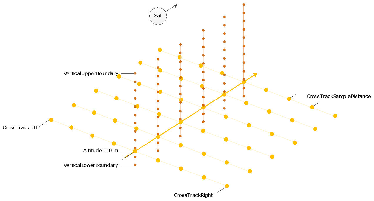
Figure 4The Joint Standard Grid X-JSG is defined by a horizontal grid with dimensions along track and across track, shown in yellow, and a vertical grid with dimensions along track and vertical, shown in orange. This is a schematic depiction with a lower number of grid points in each dimension than in the actual grid. The actual horizontal grid is somewhat more irregular due to the CPR sampling. There is somewhat larger grid spacing along track every seventh along-track pixel. Figure courtesy of X-JSG team at S[&]T (NO).
In the case that either CPR or ATLID measurement data are not available, the X-JSG processor falls back to a contingency solution. This is implemented, for instance, during instrument calibration modes. In such instances the grid will be constructed without the respective instrument, using a similar but fixed sampling. In the case of non-availability of both CPR and ATLID measurement data for a complete frame, no JSG will be produced. However, in such instances, synergistic retrievals, without measurements from the active sensors, are not required. The horizontal grid point locations define the X-JSG pixel centres. Pixels across track, for a given along-track position, share the same vertical grid. The vertical grid is specified for each grid point along track, as the position of the vertical grid points varies along track due to the dynamic adaptation of the ATLID range to the satellite height, combined with a finite step size for the range.
Along track. The spatial extent of the along-track grid is equal to a frame ( orbit), which is the granularity of all EarthCARE products. The CPR creates profile groups of 14 CPR profiles, between which there is larger spacing, which results in groups of seven X-JSG pixels. The nominal X-JSG grid is irregular due to this way of CPR sampling. In the case of no CPR measurement data, X-JSG will use a fixed 1000 m horizontal grid point distance (configurable).
Across track. Configuration parameters define a fixed 1 km grid sampling and the extent to the left and right of the ground track, selected based on MSI sampling and swath size.
Vertical. The vertical grid point distance is defined by ATLID vertical sampling, which is about 103 m up to an altitude of 20 km and about 500 m above this altitude. The lower and upper boundaries of the vertical grid are set via configuration parameters. In the case of no ATLID measurement data, a vertical grid is created with two possible vertical grid point sample distances, high resolution at 100 m sample distances and low resolution at 500 m vertical sample distances. The high- and low-resolution sample distances, as well as the altitude boundary of these sampling regions, are configurable.
This product facilitates the application of synergistic (level 2b) classification and retrieval algorithms as well as the synergistic use of a number of single-instrument (level 2a) products. It is closely linked to the merged observations product (AM-MO) which directly uses the JSG definition in order to produce a file containing co-located observations.
EarthCARE level 2 data products include a comprehensive range of geophysical parameters related to aerosols, clouds, precipitation, and radiation. Wehr et al. (2023) (Sect. 8.3) give an overview of the ESA and JAXA level 2a/level 2b data products containing retrieved aerosol, cloud, precipitation, and radiation parameters and supporting science activities. In this section we provide brief descriptions of all level 2 data products and references to corresponding publications which contain detailed information about the products, retrieval algorithms and their verification and validation. Tables 1 and 2 list all ESA and JAXA level 2a (L2a) data products, i.e. data products derived from one EarthCARE instrument only, along with the reference for their detailed description. Data products synergistically retrieved from more than one EarthCARE instrument are referred to as level 2b (L2b) data products. Inputs to level 2b processors may be level 1b/c/d data products as well as level 2a and other level 2b data products. Tables 3 and 4 list all ESA and JAXA level 2b data products, including their respective reference. All products listed in Tables 1 and 3 are operationally produced by the ESA PDGS. For products listed in Tables 2 and 4, Standard Products are operationally produced by the JAXA Satellite Applications and Operations Center (SAOC), while Research Products are products by JAXA Earth Observation Research Center (EORC) and/or Japanese institutes/universities. All products will be made available to users usually not later than 48 h after sensing.
While not part of the ESA or JAXA data products, the development of a cloud climate product processor for ATLID is relevant in this context. It is designed with the purpose of making ATLID cloud observations directly available for climate applications (Feofilov et al., 2023).
5.1 Single-instrument (level 2a) processors and products
5.1.1 ESA single-instrument processors and products
ESA data products generated from measurements of a single instrument are listed in Table 1. There is no BBR level 2a product, as scene information from the MSI is required to derive radiances and fluxes from BBR. Level 2a products are usually provided at instrument resolution or multiples thereof, ATLID and CPR on a vertical “curtain” (dimensions: along track and altitude) and MSI on a horizontal “swath” (dimensions: along track and across track).
Kollias et al. (2023)Kollias et al. (2023)Irbah et al. (2023)Mroz et al. (2023)van Zadelhoff et al. (2023a)Donovan et al. (2024)Donovan et al. (2024)Irbah et al. (2023)Donovan et al. (2024)Donovan et al. (2024)Wandinger et al. (2023)Wandinger et al. (2023)Hünerbein et al. (2023b)Hünerbein et al. (2023a)Docter et al. (2023)Table 1References of all ESA level 2a products and their retrieval algorithms shown in the ESA Production Model, Fig. 2.
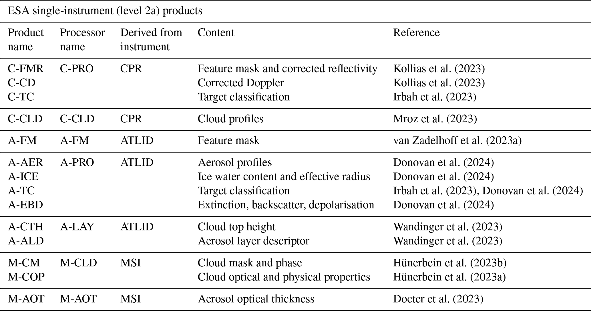
For each of the active instruments, ATLID and CPR, two classification products are produced, a feature detection mask that provides areas of significant return (A-FM and C-FMR) and a target classification that identifies various classes of hydrometeors and aerosols (A-TC and C-TC). Radar reflectivities, corrected for gaseous attenuation and non-uniform beam filling (also in C-FMR), and Doppler velocities, corrected for antenna mispointing, non-uniform beam filling, and velocity folding (C-CD), are used to derive vertical profiles of cloud and precipitation microphysical parameters (C-CLD). The primary ATLID level 2a product contains vertical profiles of extinction, backscatter, and depolarisation (A-EBD). This is the starting point for further ATLID products covering aerosol profiles (A-AER), ice cloud profiles (A-ICE), and layer information for clouds (A-CTH) and aerosols (A-ALD).
Level 2 processing for MSI also starts with a classification product (M-CM). This contains the cloud flag (i.e., cloud mask), cloud phase, and cloud type. In a second step, cloud optical and physical properties, namely cloud optical thickness, effective radius, and top height, are derived (M-COP), as well as aerosol optical thickness (M-AOT).
5.1.2 JAXA single-instrument processors and products
JAXA data products generated from measurements of a single instrument are listed in Table 2.
Hagihara et al. (2021)Hagihara et al. (2010)Kikuchi et al. (2017)Okamoto et al. (2010, 2024b)Sato and Okamoto (2011)Nishizawa et al. (2019, 2024)Hagihara et al. (2010)Yoshida et al. (2010)Okamoto et al. (2024a)Nakajima et al. (2019)Wang et al. (2023)Hagihara et al. (2021, 2023)Sato et al. (2009, 2024)Sato et al. (2009, 2024)Nishizawa et al. (2008, 2011)Letu et al. (2016, 2018)Yoshida et al. (2018)Table 2References of all JAXA level 2a products and their product category shown in the JAXA Production Model, Fig.3.
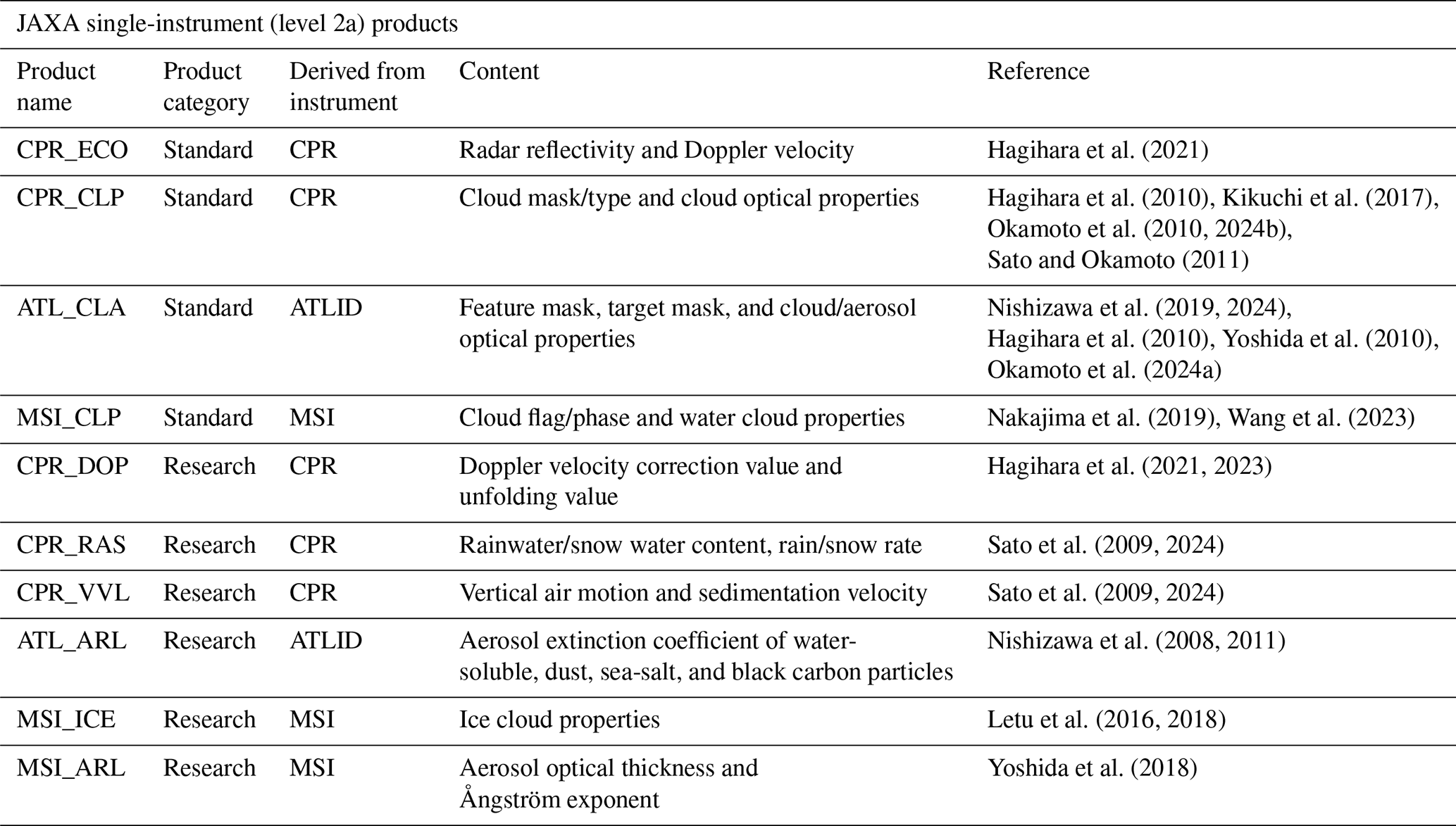
CPR_ECO, CPR_DOP, CPR_CLP, CPR_RAS, and CPR_VVL are the CPR level 2a products. CPR_ECO contains the radar reflectivity and Doppler velocity horizontally integrated over 1 and 10 km. The radar reflectivity is corrected for clutter echo and gas attenuation, and an unfolding correction is applied to the Doppler velocity. CPR_DOP provides the corrected Doppler velocity. Inhomogeneity and unfolding corrections are applied, in addition to the corrections for Doppler velocity performed in CPR_ECO. CPR_CLP contains the cloud mask, cloud particle type, and cloud microphysics, which are derived mainly from the radar reflectivity. CPR_RAS provides parameters related to rain and snow, such as rainwater content, snow water content, ratio rate, and snow rate. It also contains attenuation-corrected radar reflectivity. Two types of rainwater content and snow water content, calculated with and without Doppler velocity, are available. CPR_VVL contains the vertical air motion in cloud regions and the sedimentation velocity of cloud particles.
ATL_CLA and ATL_ARL are the ATLID level 2a products. ATL_CLA provides a target classification for each ATLID observation grid point and optical properties of cloud and aerosol, such as extinction coefficient, backscatter coefficient, lidar ratio, and depolarisation ratio. It also contains the planetary boundary layer height. ATL_ARL includes extinction coefficients for four aerosol components (dust, black carbon, sea-salt, and water-soluble particles). MSI_CLP, MSI_ICE, and MSI_ARL are the MSI level 2a products. MSI_CLP provides the cloud product derived from MSI, including cloud flag and phase information and water cloud properties, such as effective radius and optical thickness. Furthermore, cloud top temperature, pressure, and height are provided. MSI_ICE includes ice cloud properties such as optical thickness; effective radius; and cloud top temperature, pressure, and height. MSI_ARL provides aerosol optical thickness and the Ångström exponent derived from MSI. The Ångström exponent is only available over ocean.
5.2 Synergy (level 2b) processors and products
5.2.1 ESA synergy processors and products
ESA data products generated from measurements of two or more EarthCARE instruments are listed in Table 3. Level 2b products are usually provided on the Joint Standard Grid described in Sect. 4.2.
Haarig et al. (2023)Haarig et al. (2023)Velázquez Blázquez et al. (2023)Velázquez Blázquez et al. (2024)Irbah et al. (2023)Mason et al. (2023b)Cole et al. (2023)Qu et al. (2023a)Cole et al. (2023)Barker et al. (2024)Table 3References of all ESA level 2b products and their retrieval algorithms shown in the ESA Production Model, Fig. 2.
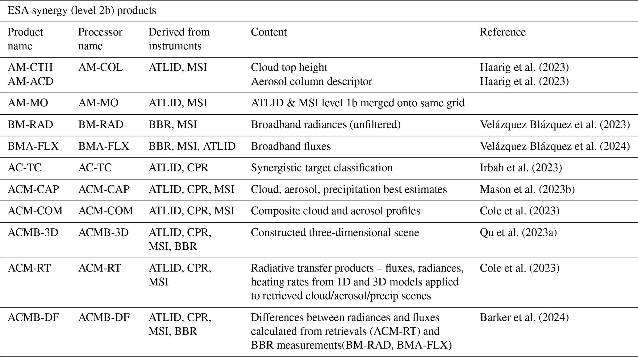
The single-instrument target classifications (A-TC and C-TC) are used to derive a synergistic target classification (AC-TC). Synergistic ATLID–MSI layer products are generated for clouds (AM-CTH) and aerosols (AM-ACD). The primary synergy product for cloud, aerosol and precipitation parameters is ACM-CAP, which uses an optimal estimation scheme. In addition, and as a backup for ACM-CAP, a simpler synergy product ACM-COM contains a best estimate of cloud and aerosol profiles based on a composite of level 2a products. As preparation to the radiative transfer calculations, a 3D scene is constructed, finding nadir pixels that match off-nadir pixels in MSI radiance (ACMB-3D). In this way, the cloud, aerosol, and precipitation fields from ACM-CAP (or as a backup, from ACM-COM) can be extended out to 15 km across track and used in 1D and 3D radiative transfer models to derive broadband radiances, fluxes, and heating rate profiles (ACM-RT). Broadband radiances (BM-RAD) and fluxes (BMA-FLX) are also derived directly from BBR measurements. In a final assessment step (ACMB-DF), broadband radiances and fluxes from radiative transfer models are compared to the ones from BBR.
5.2.2 JAXA synergy processors and products
JAXA data products generated from measurements of two or more EarthCARE instruments are listed in Table 4.
Okamoto et al. (2007, 2008, 2010)Hagihara et al. (2010)Kikuchi et al. (2017)Sato and Okamoto (2011)Okamoto et al. (2024b)Oikawa et al. (2013, 2018)Okata et al. (2017)Yamauchi et al. (2024)Sato et al. (2009, 2024)Sato et al. (2024)Sato et al. (2009, 2024)Kudo et al. (2016)Oikawa et al. (2013, 2018)Okamoto et al. (2024b)Okamoto et al. (2024b)Okamoto et al. (2024b)Okamoto et al. (2024b)Table 4References of all JAXA level 2b products and their retrieval algorithms shown in the JAXA Production Model, Fig. 3.
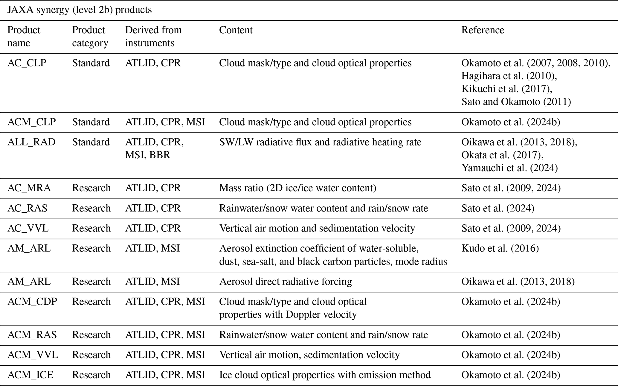
The primary synergy products for cloud and aerosol parameters are AC_CLP and ACM_CLP. AC_CLP is estimated using CPR and ATLID measurements and provides similar parameters as CPR_CLP; however, the number of grids with valid values increases compared with CPR_CLP because AC_CLP is derived from both CPR and ATLID, which have different sensitivity for thin and deep clouds. ACM_CLP is estimated using CPR, ATLID, and MSI and provides similar parameters to CPR_CLP. In addition, liquid water path and ice water path are available in ACM_CLP. Besides AC_CLP and ACM_CLP, there are several other synergy products for cloud, aerosol, and precipitation parameters. ACM_CDP utilises the Doppler velocity measured by the CPR and contains cloud mask, cloud particle type, liquid/ice water path, and cloud microphysics derived from ATLID, CPR, and MSI data. AC_MRA contains two types of mass ratio of horizontally oriented ice crystals (HOIC or 2D ice) to ice water content. One is derived with Doppler velocity and the other without Doppler velocity. AC_RAS provides rainwater content, snow water content, rain rate, and snow rate, derived from both CPR and ATLID data. Two types of rainwater content and snow water content, with and without Doppler velocity, are available. ACM_RAS contains the same parameters as AC_RAS, but ACM_RAS is derived from the three sensors ATLID, CPR, and MSI. AC_VVL provides information related to atmospheric vertical motion estimated with CPR and ATLID data. The parameters of vertical air motion and sedimentation velocity are included. ACM_VVL contains the same parameters as AC_VVL, but ACM_VVL is derived from the three sensors of ATLID, CPR, and MSI. ACM_ICE contains the effective radius and optical thickness of ice cloud, derived with the emission method called the multi-wavelength and multi-pixel (MWP) method. Radiative fluxes and heating rates are contained in ALL_RAD for both shortwave and longwave regions, derived with 1D plane-parallel radiative transfer simulations. AM_ARL provides extinction coefficients of each aerosol type (dust, black carbon, sea-salt, and water-soluble particles) and mode radii for aerosol fine and coarse modes. Aerosol direct radiative forcing at the top of the atmosphere and bottom of the atmosphere is also included.
6.1 End-To-End Simulator E3SIM
Development and testing of the processors at ESA were made possible using a dedicated EarthCARE End-to-End Simulator (E3SIM, Fig. 5). Test data, consisting of input scene files that describe the physical properties, were assembled by assimilation of data from many sources. Forward models were used to operate on the input scene files and generate the expected input to each of the instruments, with instrument models to simulate the engineering data that would be output from the instruments and transmitted to the ground. The level 0, level 1, and level 2 processors could then be used to generate the corresponding data products, which need to be compared against the input data. The E3SIM is optimised for producing small amounts of highly representative data to be used in algorithm development. It is not meant to be used for routine operational generation of data products.
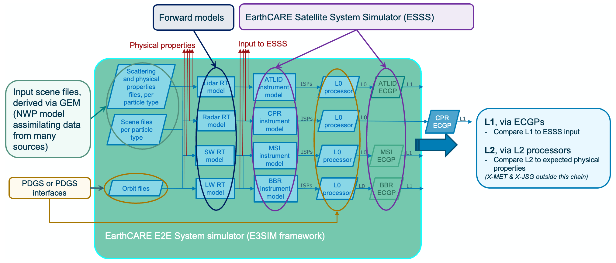
Figure 5Simulation chain developed for the EarthCARE processors development. RT: radiative transfer. SW: shortwave. LW: longwave. NWP: numerical weather prediction. E2E: End to End. ECGP: EarthCARE Ground Processor.
E3SIM consists of the simulator framework, which allows us to configure and run simulations of the complete processing chain or any part of the chain (down to individual processor runs), and the individual processor modules that are plugged into the simulator. Processors are connected to each other via their products, and outputs of one processor in the chain are inputs to one or more processors further down in the chain. The EarthCARE production model (Fig. 2) is implemented via “task tables”, which describe the inter-dependencies between processors in a general way. From these, “job orders” are generated as the basis for specific production runs, listing all required input data for a given run. This interface is the same as the one used by the operational PDGS, simplifying the development and testing as the processors only have to support a single interface.
6.2 Test data sets
The E3SIM was used to generate a number of test data sets for the processor development. Test data for level 1 processor verification used scenarios from the EarthCARE system requirements wherever possible. These typically cover the extremes of dynamic ranges, from detection limit to saturation. Level 2 processors used a wide range of input scenes, from simple synthetic scenes in the early stages of development, via scenes based on campaign data and satellite measurements, specifically the A-train instruments CloudSat, CALIPSO, and MODIS, to the three science reference frames, Halifax, Baja, and Hawaii, based on the Canadian numerical weather prediction model, GEM. This data set and its generation are described in detail by Qu et al. (2023b) and Donovan et al. (2023). It covers a wide range of cloud and aerosol scenes and was used extensively in the development, verification, and inter-comparison (Mason et al., 2023a) of the EarthCARE level 2 processors.
A data set from a global storm-resolving simulation, and its use in the global evaluation of CPR Doppler velocity errors, is described by Roh et al. (2023) and Hagihara et al. (2023).
6.3 Collaborative development
The large number of data processors and processor developers, and the complex production model with its many inter-dependencies, required an efficient setup for enabling collaboration between developers, sharing code and information, and testing and managing software problems. We used a highly integrated, collaborative software development environment, based on a mix of proprietary and open-source tools such as Atlassian Confluence for sharing information and minutes of meetings, Atlassian Jira for reporting software problems and planning work, gitea as a code repository, Jenkins for running automated tests, and MinIO as a test data repository.
6.4 Lessons learnt
After more than 15 years of developing the EarthCARE processing system at ESA, it is useful to look back and reflect on what could have been done better and what worked well.
We found that it is important to systematically build up the end-to-end simulation chain and keep it consistent along the way. Interfaces and reference software environments should be defined and documented very early. It is useful not to develop everything in parallel from the start but instead to build a single chain first (preferably the one for the “simplest” instrument) and then review what can be improved, feed that into general requirements, and apply the lessons learned to remaining chains (which can then be done in parallel). Interfaces need to be standardised and defined early, and level 1 processors need to be connected to the level 2 processing chain early, allowing sufficient time for feedback from the level 2 developments to the level 1 algorithms. Instrument calibration data will always be available relatively late in the development process; therefore it is important to have good proxies for these data available early and to update them systematically as new information about instrument performance becomes available.
Consistency of the simulation and processing chain (including input data) should be verified regularly. Fundamental changes in the processing chain at a late stage of the development must be avoided. If they do happen, they must include a corresponding adaptation of other parts of the chain to keep it consistent (example: level 1 processor update might require an instrument simulator update).
Expertise and developments should be organised “vertically” along instrument processing chains (e.g. ATLID, CPR) rather than “horizontally” along processing levels (e.g. instrument simulator, level 1 processor). This is to account for strong interdependencies between processors along instrument processing chains (“vertically”) which require close interaction of the involved experts, specifically instrument developers and level 2 processor developers, particularly for active instruments where instrument expertise and geophysical expertise need to be combined in order to achieve the best possible calibration of the instrument and its level products. Consistency across instruments (“horizontally”) is important as well but can and should be organised and monitored separately.
Test data sets should be systematically built up and curated in a dedicated and not to be underestimated effort along the development. Rigorous configuration control is required for test data sets (including the CCDB), making them fully traceable. Test data set limitations (examples: simplistic assumptions made when generating the data set, format non-compliances, undefined parameters in the data product, non-usability for a certain purpose) should be documented at every development step. Test data should contain (i) synthetic, simple test data sets, allowing simple verification and code debugging along the development process; (ii) data sets using actual instrument data (in particular for internal calibration modes); (iii) state-of-the art simulated scientific data sets covering at least one orbit; and (iv) long data sets (up to a full repeat cycle) for ground-segment verification and pre-launch rehearsals.
Master repositories should be used for code, test data, and documentation. The same item should not be stored in multiple places (other than synchronised repositories for backup).
Level 2 processor developers should be involved early in the level 1 algorithm/product verification, with bread-boarding of critical modules. Development contracts should be short (not longer than 2.5 years) to keep flexibility. Agile software developments, whereby working code is frequently delivered and discussed, and requirements are allowed to evolve, worked very well for EarthCARE. All delivered code needs to be used immediately, regularly, and by as many people as possible, so issues can be identified and fixed early, while software developers are still familiar with the code.
We found that it worked well to have a set of general requirements and conventions across all processors, to have a common reference software environment for all processors, and to limit allowed programming languages to the absolute minimum (for EarthCARE: C/C++/Fortran); this simplified the maintenance. Strict processor runtime requirements turned out to be very useful, forcing developers to optimise runtime. We had an efficient setup of software support to the scientific level 2 processor developers, and the collaborative environment described in the previous section helped to coordinate the development in an efficient way.
We have presented an overview of the EarthCARE processors development, encompassing processors developed by teams in Europe, Japan, and Canada. These will facilitate exploitation of the four instruments embarked on the EarthCARE satellite, which will fly in a sun-synchronous, low-Earth orbit with a mean local solar time of 14:00 ±5 min. As well as the single instrument products available at level 1 and level 2, a comprehensive set of multiple-instrument, synergistic, level 2 data products will retrieve aerosol, cloud, precipitation, and radiation parameters. A Joint Standard Grid is generated and used to ensure that radar, lidar, and multispectral image data are collocated such that the same column of the atmosphere is viewed. An auxiliary product contains a subset of meteorological fields from an ECMWF atmospheric model that covers the EarthCARE swath.
Testing of the processing chain at ESA has made use of a dedicated End-to-End Simulator, called E3SIM, and special test data sets that were generated from data assimilated from multiple sources. E3SIM incorporates forward models and instrument simulators to generate the signals expected in Instrument Source Packets. The ISPs are ingested into the processor chain, and outputs can be compared against the input data. A description of the collaborative development used in the processing chain development was presented as well as the lessons learnt.
An overview was given of the EarthCARE product format and conventions, as well as a short summary of the different products' contents and references to the dedicated papers that describe their algorithm and content in more detail. All EarthCARE data products will be available from both ESA and JAXA websites.
EarthCARE will allow scientists to evaluate the representation of cloud, aerosol, precipitation, and radiative flux in weather forecast and climate models, with the objective to improve parameterisations and, in particular, address uncertainties in cloud processes.
For EarthCARE product names (acronyms containing a hyphen or underscore), see Tables 1 to 4.
| ATLID | Atmospheric lidar |
| BBR | Broadband Radiometer |
| CALIPSO | Cloud-Aerosol Lidar and Infrared Pathfinder Satellite Observations |
| CCDB | Calibration and Characterisation Database |
| CERES | Clouds and Earth's Radiant Energy System |
| CPR | Cloud Profiling Radar |
| CSC | Coarse spectral calibration |
| DCC | Dark-current calibration |
| E3SIM | EarthCARE End-to-End Simulator |
| ECGP | EarthCARE Ground Processor |
| ECMWF | European Centre for Medium-Range Weather Forecasts |
| EORC | Earth Observation Research Center |
| FSC | Fine spectral calibration |
| GEM | Global Environmental Multiscale Model |
| HOIC | Horizontally oriented ice crystals |
| HRES | High resolution |
| ICMF | Instrument Calibration and Monitoring Facility |
| ICU | Instrument Control Unit |
| IFS | Integrated Forecast System |
| ISP | Instrument Source Packet (or Instrument Science Packet) |
| JSG | Joint Standard Grid |
| MODIS | Moderate Resolution Imaging Spectroradiometer |
| MSI | Multi-Spectral Imager |
| MWP | Multi-wavelength and multi-pixel |
| NEdT | Noise-equivalent differential temperature |
| NRCS | Normalised (surface scattering) radar cross section |
| NWP | Numerical weather prediction |
| Point distribution function | |
| PDGS | Payload Data Ground Segment |
| PRF | Pulse repetition frequency |
| SAOC | Satellite Applications and Operations Center |
| TDI | Time delay integration |
| TIR | Thermal infrared |
| VNS | Visible near-infrared shortwave-infrared |
| WGS | World Geodetic System |
| WMO | World Meteorological Organization |
This overview paper refers generally to software code for level 2 processors and for atmospheric models that have been used to prepare data and simulations. The references for software repositories can be found in each of the dedicated papers that are contained within this special issue on EarthCARE level 2 algorithms and data products. The EarthCARE level 2 demonstration products from simulated scenes are available at https://doi.org/10.5281/zenodo.7117115 (van Zadelhoff et al., 2023b).
ME prepared the manuscript and processing chain and development sections. FM described the ATLID and BBR instrument and level 1 processors. KW introduced the mission and described the MSI instrument and level 1 processor and the auxiliary processors. TK described the CPR instrument and level 1 processor, with contributions from NT and YO. TT described the JAXA level 2 processing chain. TW contributed to the science background and data product overview. DB, the ESA EarthCARE Project Manager, and ET, the JAXA Project Manager, provided overall guidance on the technical and programmatic context.
The contact author has declared that none of the authors has any competing interests.
Publisher’s note: Copernicus Publications remains neutral with regard to jurisdictional claims made in the text, published maps, institutional affiliations, or any other geographical representation in this paper. While Copernicus Publications makes every effort to include appropriate place names, the final responsibility lies with the authors.
This article is part of the special issue ”EarthCARE level 2 algorithms and data products”. It is not associated with a conference.
We would like to recognise the industrial partners working on the satellite, payload and level 1 processors, led by the satellite prime, Airbus Defence and Space (Germany), with instrument teams at NEC (Japan), SSTL (UK), Airbus Defence and Space (France), Thales Alenia Space (UK), and level 1 processors development and auxiliary processors development supported by GMV (UK) and S[&]T (NO) respectively. We thank the teams of scientists at several institutions in Europe, Japan, and Canada that have developed EarthCARE level 2 processors and products, as well as at the ECMWF. Special thanks are given to members of the Joint Mission Advisory Group, which advises ESA and JAXA on science aspects of the mission, as well as to the principal investigators and project scientists of NASA missions CloudSat and CALIPSO and the CERES instrument for their long-standing support and advice. We would also like to thank colleagues at ESA, JAXA, and NICT and particularly remember our friend and colleague Tobias Wehr, EarthCARE mission scientist, who passed away suddenly and unexpectedly in 2023, after more than a decade of support of the mission.
This paper was edited by Ulla Wandinger and reviewed by three anonymous referees.
Barker, H. W., Cole, J. N. S., Qu, Z., Villefranque, N., Hogan, R., and Mason, S.: Radiative closure assessment of retrieved cloud and aerosol properties for the EarthCARE mission: the ACMB-DF product, Atmos. Meas. Tech., in preparation, 2024. a, b
Cole, J. N. S., Barker, H. W., Qu, Z., Villefranque, N., and Shephard, M. W.: Broadband radiative quantities for the EarthCARE mission: the ACM-COM and ACM-RT products, Atmos. Meas. Tech., 16, 4271–4288, https://doi.org/10.5194/amt-16-4271-2023, 2023. a, b
Docter, N., Preusker, R., Filipitsch, F., Kritten, L., Schmidt, F., and Fischer, J.: Aerosol optical depth retrieval from the EarthCARE Multi-Spectral Imager: the M-AOT product, Atmos. Meas. Tech., 16, 3437–3457, https://doi.org/10.5194/amt-16-3437-2023, 2023. a
Donovan, D. P., Kollias, P., Velázquez Blázquez, A., and van Zadelhoff, G.-J.: The generation of EarthCARE L1 test data sets using atmospheric model data sets, Atmos. Meas. Tech., 16, 5327–5356, https://doi.org/10.5194/amt-16-5327-2023, 2023. a
Donovan, D. P., van Zadelhoff, G.-J., and Wang, P.: The EarthCARE lidar cloud and aerosol profile processor: the A-AER, A-EBD, A-TC and A-ICE products, Atmos. Meas. Tech., submitted, 2024. a, b, c, d
Feofilov, A. G., Chepfer, H., Noël, V., and Szczap, F.: Incorporating EarthCARE observations into a multi-lidar cloud climate record: the ATLID (Atmospheric Lidar) cloud climate product, Atmos. Meas. Tech., 16, 3363–3390, https://doi.org/10.5194/amt-16-3363-2023, 2023. a
Haarig, M., Hünerbein, A., Wandinger, U., Docter, N., Bley, S., Donovan, D., and van Zadelhoff, G.-J.: Cloud top heights and aerosol columnar properties from combined EarthCARE lidar and imager observations: the AM-CTH and AM-ACD products, EGUsphere [preprint], https://doi.org/10.5194/egusphere-2023-327, 2023. a, b
Hagihara, Y., Okamoto, H., and Yoshida, R.: Development of a combined CloudSat-CALIPSO cloud mask to show global cloud distribution, J. Geophys. Res., 115, D00H33, https://doi.org/10.1029/2009JD012344, 2010. a, b, c
Hagihara, Y., Ohno, Y., Horie, H., Roh, W., Satoh, M., Kubota, T., and Oki, R.: Assessments of Doppler Velocity Errors of EarthCARE Cloud Profiling Radar Using Global Cloud System Resolving Simulations: Effects of Doppler Broadening and Folding, IEEE T. Geosci. Remote, 60, 1–9, 2021. a, b
Hagihara, Y., Ohno, Y., Horie, H., Roh, W., Satoh, M., and Kubota, T.: Global evaluation of Doppler velocity errors of EarthCARE cloud-profiling radar using a global storm-resolving simulation, Atmos. Meas. Tech., 16, 3211–3219, https://doi.org/10.5194/amt-16-3211-2023, 2023. a, b
Hünerbein, A., Bley, S., Deneke, H., Meirink, J. F., van Zadelhoff, G.-J., and Walther, A.: Cloud optical and physical properties retrieval from EarthCARE multi-spectral imager: the M-COP products, EGUsphere [preprint], https://doi.org/10.5194/egusphere-2023-305, 2023a. a
Hünerbein, A., Bley, S., Horn, S., Deneke, H., and Walther, A.: Cloud mask algorithm from the EarthCARE Multi-Spectral Imager: the M-CM products, Atmos. Meas. Tech., 16, 2821–2836, https://doi.org/10.5194/amt-16-2821-2023, 2023b. a
IPCC: Climate Change 2021 – The Physical Science Basis: Working Group I Contribution to the Sixth Assessment Report of the Intergovernmental Panel on Climate Change, edited by: Masson-Delmotte, V., Zhai, P., Pirani, A., Connors, S. L., Péan, C., Berger, S., Caud, N., Chen, Y., Goldfarb, L., Gomis, M. I., Huang, M., Leitzell, K., Lonnoy, E., Matthews, J. B. R., Maycock, T. K., Waterfield, T., Yelekçi, O., Yu, R., and Zhou, B., Cambridge University Press, Cambridge, United Kingdom and New York, NY, USA, https://doi.org/10.1017/9781009157896, 2023. a
Irbah, A., Delanoë, J., van Zadelhoff, G.-J., Donovan, D. P., Kollias, P., Puigdomènech Treserras, B., Mason, S., Hogan, R. J., and Tatarevic, A.: The classification of atmospheric hydrometeors and aerosols from the EarthCARE radar and lidar: the A-TC, C-TC and AC-TC products, Atmos. Meas. Tech., 16, 2795–2820, https://doi.org/10.5194/amt-16-2795-2023, 2023. a, b, c
Kikuchi, M., Okamoto, H., Sato, K., Suzuki, K., Cesana, G., Hagihara, Y., Takahashi, N., Hayasaka, T., and Oki, R.: Development of algorithm for discriminating hydrometeor particle types with a synergistic Use of CloudSat and CALIPSO, J. Geophys. Res.-Atmos., 122, 11022–11044, 2017. a, b
Kollias, P., Puidgomènech Treserras, B., Battaglia, A., Borque, P. C., and Tatarevic, A.: Processing reflectivity and Doppler velocity from EarthCARE's cloud-profiling radar: the C-FMR, C-CD and C-APC products, Atmos. Meas. Tech., 16, 1901–1914, https://doi.org/10.5194/amt-16-1901-2023, 2023. a, b
Kudo, R., Nishizawa, T., and Aoyagi, T.: Vertical profiles of aerosol optical properties and the solar heating rate estimated by combining sky radiometer and lidar measurements, Atmos. Meas. Tech., 9, 3223–3243, https://doi.org/10.5194/amt-9-3223-2016, 2016. a
Letu, H., Ishimoto, H., Riedi, J., Nakajima, T. Y., C.-Labonnote, L., Baran, A. J., Nagao, T. M., and Sekiguchi, M.: Investigation of ice particle habits to be used for ice cloud remote sensing for the GCOM-C satellite mission, Atmos. Chem. Phys., 16, 12287–12303, https://doi.org/10.5194/acp-16-12287-2016, 2016. a
Letu, H., Nagao, T. M., Nakajima, T. Y., Riedi, J., Ishimoto, H., Baran, A. J., Shang, H., Sekiguchi, M., and Kikuchi, M.: Ice cloud properties from Himawari-8/AHI next-generation geostationary satellite: Capability of the AHI to monitor the DC cloud generation process, IEEE T. Geosci. Remote, 57, 3229–3239, 2018. a
Mason, S. L., Cole, J. N. S., Docter, N., Donovan, D. P., Hogan, R. J., Hünerbein, A., Kollias, P., Puigdomènech Treserras, B., Qu, Z., Wandinger, U., and van Zadelhoff, G.-J.: An intercomparison of EarthCARE cloud, aerosol and precipitation retrieval products, EGUsphere [preprint], https://doi.org/10.5194/egusphere-2023-1682, 2023a. a
Mason, S. L., Hogan, R. J., Bozzo, A., and Pounder, N. L.: A unified synergistic retrieval of clouds, aerosols, and precipitation from EarthCARE: the ACM-CAP product, Atmos. Meas. Tech., 16, 3459–3486, https://doi.org/10.5194/amt-16-3459-2023, 2023b. a
Mroz, K., Treserras, B. P., Battaglia, A., Kollias, P., Tatarevic, A., and Tridon, F.: Cloud and precipitation microphysical retrievals from the EarthCARE Cloud Profiling Radar: the C-CLD product, Atmos. Meas. Tech., 16, 2865–2888, https://doi.org/10.5194/amt-16-2865-2023, 2023. a
Nakajima, T. Y., Ishida, H., Nagao, T. M., Hori, M., Letu, H., Higuchi, R., Tamaru, N., Imoto, N., and Yamazaki, A.: Theoretical basis of the algorithms and early phase results of the GCOM-C (Shikisai) SGLI cloud products, Progress in Earth and Planetary Science, 6, 1–25, 2019. a
Nishizawa, T., Sugimoto, N., Matsui, I., Shimizu, A., Tatarov, B., and Okamoto, H.: Algorithm to retrieve aerosol optical properties from high-spectral-resolution lidar and polarization Mie-scattering lidar measurements, IEEE T. Geosci. Remote, 46, 4094–4103, 2008. a
Nishizawa, T., Sugimoto, N., Matsui, I., Shimizu, A., and Okamoto, H.: Algorithms to retrieve optical properties of three component aerosols from two-wavelength backscatter and one-wavelength polarization lidar measurements considering nonsphericity of dust, J. Quant. Spectrosc. Ra., 112, 254–267, 2011. a
Nishizawa, T., Kudo, R., Higure, A., Oikawa, E., and Hajime, O.: Aerosol and Cloud Retrieval Algorithms Using EarthCARE Satellite-borne Lidar Data, J. Remote Sensing Society of Japan, 39, 215–224, https://doi.org/10.11440/rssj.39.215, 2019 (in Japanese). a
Nishizawa, T., Kudo, R., Oikawa, E., Higurashi, A., Jin, Y., Takakura, S., Sugimoto, N., Fujikawa, M., Sato, K., and Okamoto, H.: Retrieval of aerosol optical properties from the EarthCARE high-spectral resolution lidar measurements, Atmos. Meas. Tech., in preparation, 2024. a
Oikawa, E., Nakajima, T., Inoue, T., and Winker, D.: A study of the shortwave direct aerosol forcing using ESSP/CALIPSO observation and GCM simulation, J. Geophys. Res.-Atmos., 118, 3687–3708, 2013. a, b
Oikawa, E., Nakajima, T., and Winker, D.: An evaluation of the shortwave direct aerosol radiative forcing using CALIOP and MODIS observations, J. Geophys. Res.-Atmos., 123, 1211–1233, 2018. a, b
Okamoto, H., Nishizawa, T., Takemura, T., Kumagai, H., Kuroiwa, H., Sugimoto, N., Matsui, I., Shimizu, A., Emori, S., Kamei, A., and Nakajima, T.: Vertical cloud structure observed from shipborne radar and lidar: Midlatitude case study during the MR01/K02 cruise of the research vessel Mirai, J. Geophys. Res., 112, D08216, https://doi.org/10.1029/2006JD007628, 2007. a
Okamoto, H., Nishizawa, T., Takemura, T., Sato, K., Kumagai, H., Ohno, Y., Sugimoto, N., Shimizu, A., Matsui, I., and Nakajima, T.: Vertical cloud properties in the tropical western Pacific Ocean: Validation of the CCSR/NIES/FRCGC GCM by shipborne radar and lidar, J. Geophys. Res.-Atmos., 113, D24213, https://doi.org/10.1029/2008JD009812, 2008. a
Okamoto, H., Sato, K., and Hagihara, Y.: Global analysis of ice microphysics from CloudSat and CALIPSO: Incorporation of specular reflection in lidar signals, J. Geophys. Res.-Atmos., 115, D22209, https://doi.org/10.1029/2009JD013383, 2010. a, b
Okamoto, H., Sato, K., Oikawa, E., Hagihara, Y., Shaik, A., and Nishizawa, T.: Cloud mask and particle type classification using EarthCARE CPR and ATLID, Atmos. Meas. Tech., in preparation, 2024a. a
Okamoto, H., Sato, K., Oikawa, E., Ishimoto, H., Ohno, Y., Horie, H., Hagihara, Y., Nishizawa, T., Kudo, R., Higurashi, A., Jin, Y., Nakajima, T. Y., Wang, M., Roh, W., Satoh, M., Suzuki, K., Kubota, T., Tanaka, T., Yamauchi, A., Sekiguchi, M., and Nagao, T. M.: Overview of EarthCARE JAXA Level 2 algorithms, Atmos. Meas. Tech., in preparation, 2024b. a, b, c, d, e, f
Okata, M., Nakajima, T., Suzuki, K., Inoue, T., Nakajima, T., and Okamoto, H.: A study on radiative transfer effects in 3-D cloudy atmosphere using satellite data, J. Geophys. Res.-Atmos., 122, 443–468, 2017. a
Qu, Z., Barker, H. W., Cole, J. N. S., and Shephard, M. W.: Across-track extension of retrieved cloud and aerosol properties for the EarthCARE mission: the ACMB-3D product, Atmos. Meas. Tech., 16, 2319–2331, https://doi.org/10.5194/amt-16-2319-2023, 2023a. a
Qu, Z., Donovan, D. P., Barker, H. W., Cole, J. N. S., Shephard, M. W., and Huijnen, V.: Numerical model generation of test frames for pre-launch studies of EarthCARE's retrieval algorithms and data management system, Atmos. Meas. Tech., 16, 4927–4946, https://doi.org/10.5194/amt-16-4927-2023, 2023b. a
Roh, W., Satoh, M., Hashino, T., Matsugishi, S., Nasuno, T., and Kubota, T.: Introduction to EarthCARE synthetic data using a global storm-resolving simulation, Atmos. Meas. Tech., 16, 3331–3344, https://doi.org/10.5194/amt-16-3331-2023, 2023. a
Sato, K. and Okamoto, H.: Refinement of global ice microphysics using spaceborne active sensors, J. Geophys. Res.-Atmos., 116, D20202, https://doi.org/10.1029/2011JD015885, 2011. a, b
Sato, K., Okamoto, H., Yamamoto, M. K., Fukao, S., Kumagai, H., Ohno, Y., Horie, H., and Abo, M.: 95-GHz Doppler radar and lidar synergy for simultaneous ice microphysics and in-cloud vertical air motion retrieval, J. Geophys. Res.-Atmos., 114, D03203, https://doi.org/10.1029/2008JD010222, 2009. a, b, c, d
Sato, K., Okamoto, H., Nishizawa, T., Ishimoto H., and Nakajima, T.: Cloud and precipitation microphysics retrievals from EarthCARE CPR, ATLID and MSI, Atmos. Meas. Tech., in preparation, 2024. a, b, c, d, e
van Zadelhoff, G.-J., Donovan, D. P., and Wang, P.: Detection of aerosol and cloud features for the EarthCARE atmospheric lidar (ATLID): the ATLID FeatureMask (A-FM) product, Atmos. Meas. Tech., 16, 3631–3651, https://doi.org/10.5194/amt-16-3631-2023, 2023a. a
van Zadelhoff, G.-J., Barker, H. W., Baudrez, E., Bley, S., Clerbaux, N., Cole, J. N. S., de Kloe, J., Docter, N., Domenech, C., Donovan, D. P., Dufresne, J.-L., Eisinger, M., Fischer, J., García-Marañón, R., Haarig, M., Hogan, R. J., Hünerbein, A., Kollias, P., Koopman, R., Madenach, N., Mason, S. L., Preusker, R., Puigdomènech Treserras, B., Qu, Z., Ruiz-Saldaña, M., Shephard, M., Velázquez-Blazquez, A., Villefranque, N., Wandinger, U., Wang, P., and Wehr, T.: EarthCARE level-2 demonstration products from simulated scenes, Zenodo [data set], https://doi.org/10.5281/zenodo.7117115, 2023b. a
Velázquez Blázquez, A., Baudrez, E., Clerbaux, N., and Domenech, C.: Unfiltering of the EarthCARE Broadband Radiometer (BBR) observations: the BM–RAD product, Atmos. Meas. Tech. Discuss. [preprint], https://doi.org/10.5194/amt-2023-170, in review, 2023. a, b
Velázquez Blázquez, A., Baudrez, E., Clerbaux, N., Domenech, C., Madenach, N., Marañón, R. G., and Salas Molar, C.: Retrieval of top-of-atmosphere fluxes from combined EarthCARE lidar, imager and broadband radiometer observations: the BMA-FLX product, Atmos. Meas. Tech., in preparation, 2024. a
Wandinger, U., Haarig, M., Baars, H., Donovan, D., and van Zadelhoff, G.-J.: Cloud top heights and aerosol layer properties from EarthCARE lidar observations: the A-CTH and A-ALD products, Atmos. Meas. Tech., 16, 4031–4052, https://doi.org/10.5194/amt-16-4031-2023, 2023. a, b
Wang, M., Nakajima, T. Y., Roh, W., Satoh, M., Suzuki, K., Kubota, T., and Yoshida, M.: Evaluation of the spectral misalignment on the Earth Clouds, Aerosols and Radiation Explorer/multi-spectral imager cloud product, Atmos. Meas. Tech., 16, 603–623, https://doi.org/10.5194/amt-16-603-2023, 2023. a
Wehr, T., Kubota, T., Tzeremes, G., Wallace, K., Nakatsuka, H., Ohno, Y., Koopman, R., Rusli, S., Kikuchi, M., Eisinger, M., Tanaka, T., Taga, M., Deghaye, P., Tomita, E., and Bernaerts, D.: The EarthCARE mission – science and system overview, Atmos. Meas. Tech., 16, 3581–3608, https://doi.org/10.5194/amt-16-3581-2023, 2023. a, b, c, d, e
Yamauchi, A., Suzuki, K., Oikawa, E., Sekiguchi, M., and Nagao, T. M.: Description and validation of the Japanese algorithms for radiative flux and heating rate products with all four EarthCARE instruments, Atmos. Meas. Tech., in preparation, 2024. a
Yoshida, M., Kikuchi, M., Nagao, T. M., Murakami, H., Nomaki, T., and Higurashi, A.: Common retrieval of aerosol properties for imaging satellite sensors, J. Meteorol. Soc. Jpn., Ser. II, 96B, 193–209, https://doi.org/10.2151/jmsj.2018-039, 2018. a
Yoshida, R., Okamoto, H., Hagihara, Y., and Ishimoto, H.: Global analysis of cloud phase and ice crystal orientation from Cloud-Aerosol Lidar and Infrared Pathfinder Satellite Observation (CALIPSO) data using attenuated backscattering and depolarization ratio, J. Geophys. Res.-Atmos, 115, D00H32, https://doi.org/10.1029/2009JD012334, 2010. a
- Abstract
- Introduction
- Processing chains
- Level 1 data processors and products
- Auxiliary data (level 1d) processors and products
- Level 2 data processors and products
- Development of the EarthCARE processing chain
- Conclusions
- Appendix A: List of acronyms
- Code and data availability
- Author contributions
- Competing interests
- Disclaimer
- Special issue statement
- Acknowledgements
- Review statement
- References