Long-term aerosol particle depolarization ratio measurements with HALO Photonics Doppler lidar

It has been demonstrated that HALO Photonics Doppler lidars (denoted HALO Doppler lidar hereafter) have the capability for retrieving the aerosol particle depolarization ratio at a wavelength of 1565 nm. For these lidars operating at such a long wavelength, the retrieval quality depends to a large degree on an accurate representation of the instrumental noise floor and the performance of the internal polarizer, whose stability has not yet been assessed for long-term operation. Here, we use 4 years of measurements at four sites in Finland to investigate the long-term performance of HALO Doppler lidars, focusing on aerosol particle depolarization ratio retrieval. The instrumental noise level, represented by noise-only signals in aerosol- and hydrometeor-free regions, shows stable performance for most instruments but clear differences between individual instruments. For all instruments, the polarizer bleed-through evaluated at liquid cloud base remains reasonably constant at approximately 1 % with a standard deviation of less than 1 %. We find these results to be sufficient for long-term aerosol particle depolarization ratio measurements and proceed to analyse the seasonal and diurnal cycles of the aerosol particle depolarization ratio in different environments in Finland, including in the Baltic Sea archipelago, a boreal forest and rural sub-arctic. To do so, we further develop the background correction method and construct an algorithm to distinguish aerosol particles from hydrometeors. The 4-year averaged aerosol particle depolarization ratio ranges from 0.07 in sub-arctic Sodankylä to 0.13 in the boreal forest in Hyytiälä. At all sites, the aerosol particle depolarization ratio is found to peak during spring and early summer, even exceeding 0.20 at the monthly-mean level, which we attribute to a substantial contribution from pollen. Overall, our observations support the long-term usage of HALO Doppler lidar depolarization ratio measurements, including detection of aerosols that may pose a safety risk for aviation.

1 Introduction

Information on the aerosol vertical distribution in the atmosphere is vital for many applications. For instance, the direct radiative effects of aerosols can be quite different if the aerosol layer is situated above a cloud layer rather than within the boundary layer, while aerosol indirect radiative effects occur only if aerosols are immersed within the cloud (IPCC, 2021). The impact of aerosol on clouds and the radiative balance of the Earth are among the largest uncertainties in our understanding (IPCC, 2021). Air quality and associated adverse health effects (Di et al., 2017) are determined by surface concentrations, which, however, are strongly affected by the vertical structure of the boundary layer (Kanawade et al., 2020; Wang et al., 2020). Finally, from an aviation point of view, high-resolution profiles of aerosol vertical distribution could play a crucial role in mitigating the impact of hazardous aerosol emissions (Hirtl et al., 2020).

Aerosol vertical profiles can be observed with a number of different methods, such as in situ instruments mounted on different platforms including research and commercial aircraft (Johnson et al., 2008; Pratt and Prather, 2010), tethered balloons (Rankin and Wolff, 2002; Hara et al., 2013; Creamean et al., 2021), hot-air balloons (Petäjä et al., 2012), zeppelin (Rosati et al., 2016) and UAVs (Brus et al., 2021; Mamali et al., 2018). Comprehensive aerosol properties can be obtained from in situ measurements (mass, size distribution and chemical composition), but the capabilities of the chosen platform limit the temporal resolution at which profiles can be obtained as well as the vertical extent of the profiling. On the other hand, active remote sensing with lidar only retrieves the optical properties of aerosol but is capable of continuous observations of the vertical structure of the atmosphere. Space-borne lidars such as CALIPSO (Cloud-Aerosol Lidar and Infrared Pathfinder Satellite Observation; Winker et al., 2009) cover the globe but with low temporal and spatial resolutions due to their very narrow swath. Airborne lidars, such as HSRL-1 (High Spectral Resolution Lidar) built and operated by NASA Langley Research Center (Hair et al., 2008), provide good spatial coverage but are costly and only able to operate for a relatively short period at a time. A combination of temporal and spatial coverage can be achieved through ground-based networks of lidars, such as EARLINET (European Aerosol Research Lidar Network; Pappalardo et al., 2014) and Finland's ground-based remote-sensing network (Hirsikko et al., 2014). These lidar networks enable the monitoring in real-time of the aerosol vertical profiles in different environments across a large area. Consequently, they facilitate the detection of elevated aerosol layers and the investigation of long-term vertical atmospheric properties.

In active remote sensing, one of the most important parameters for characterizing aerosol is the particle depolarization ratio (denoted as δ), which is the ratio of the co-polar and cross-polar signals backscattered from aerosol. This parameter is used to distinguish between spherical and non-spherical particles (Burton et al., 2012; Mamouri and Ansmann, 2016; Baars et al., 2017) and is therefore essential in differentiating aerosol types (Illingworth et al., 2015) such as smoke, dust, marine and ash. Typically, the δ of aerosol is measured at shorter wavelengths such as at 355, 523, 532, 694, 710 or 1064 nm (Murayama et al., 2001; Sassen, 2002; Engelmann et al., 2016; Baars et al., 2016). This study is conducted using data from HALO Doppler lidars at 1565 nm, which is a relatively new addition to the suite of wavelengths used for the δ of aerosol retrieval (Vakkari et al., 2021).

HALO Doppler lidars (Pearson et al., 2009) are the core remote sensing instruments in the Finnish ground-based remote sensing network. In this study, we analysed data from these instruments at four different locations in the network from 2016 to 2019. Liquid clouds were identified, and the δ at liquid cloud base was collected to derive the depolarization bleed-through (Vakkari et al., 2021) and its temporal evolution for five different HALO Doppler lidar instruments. In addition, the stability of every HALO Doppler lidar in the network was also assessed through the time series of the signal-to-noise ratio in aerosol- and hydrometeor-free regions. Furthermore, an aerosol identification algorithm was created to enable the separation of aerosol and hydrometeors, similar to the Cloudnet algorithm (Illingworth et al., 2007; Tukiainen et al., 2020), but based only on one instrument. The algorithm was used to extract the δ in the aerosol region (δ of aerosol) at all locations and, subsequently, the overall statistics of the δ of aerosol at 1565 nm in Finland across 4 years. These statistics can improve aviation safety by providing a baseline of the δ of aerosol at this wavelength so that potentially hazardous layers such as smoke and volcanic ash can be separated from the natural aerosol more easily.

2 Materials and methods

2.1 HALO Doppler lidar

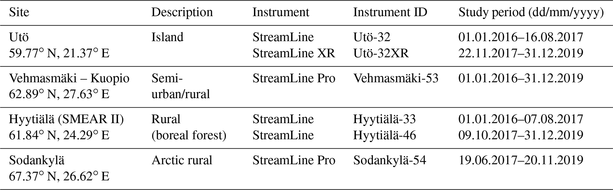
The Finnish remote sensing network deploys HALO Doppler lidars in several measurement stations across Finland (Hirsikko et al., 2014). This study uses data from Utö, Hyytiälä, Vehmasmäki and Sodankylä (Fig. 1). Each location has a different environment, enabling comparisons between both urban and rural, as well as marine, continental, and sub-arctic regions. Detailed descriptions and the study period for each location are shown in Table 1.

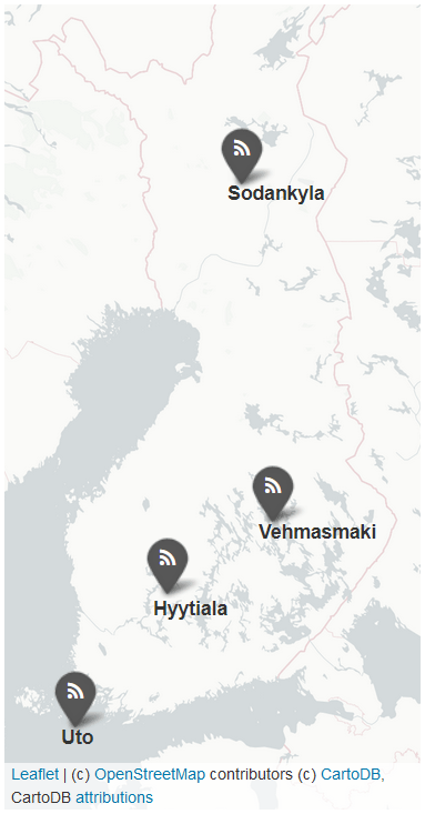
Figure 1 Locations of the instruments across Finland.

Table 1 Description of instrument locations.

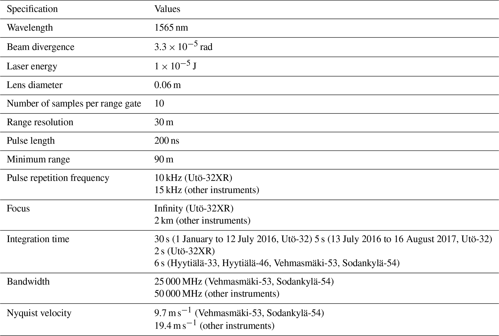
The HALO Photonics StreamLine Doppler lidars (denoted HALO Doppler lidars), operated by the Finnish Meteorological Institute, are 1565 nm pulsed Doppler lidars transmitting linearly polarized light and equipped with heterodyne detectors that can switch between recording the return in two channels parallel and orthogonal with respect to the transmitted polarization (Pearson et al., 2009), termed co-polar (parallel) and cross-polar (orthogonal). These lidars are fibre optic systems, utilizing solid-state lasers, and are capable of operating continuously for a long period of time (Harvey et al., 2013). In addition, these systems conform to eye-safety requirements as they operate at high-pulse repetition and low-pulse energy mode with a 1565 nm laser (Pearson et al., 2009).

Three versions of HALO Doppler lidars are utilized in this study: StreamLine, StreamLine Pro and StreamLine XR lidars. The StreamLine and StreamLine XR lidars are capable of full hemispheric scanning. Designed for harsher environments, the StreamLine Pro lidar has no external moving parts, limiting the scanning to within a 20^∘ cone around zenith. The StreamLine XR has higher power and a lower pulse repetition frequency and thus can observe up to 12 km in range above ground level (a.g.l.) compared to only 9.6 km for the StreamLine and Streamline Pro. Key specifications of all instruments are shown in Table 2.

Table 2 Instrument configurations.

The operational mode of each instrument varies with location. The standard operation mode consists of continuous vertical staring with periodical switching to velocity-azimuth display scans for obtaining vertical profiles of the horizontal wind. For about 10–30 s in every hour, the instruments perform a periodical background noise determination. Only data from the vertical staring mode are utilized in this study, so occasional gaps in data availability are due to lower-elevation angle scanning and the background noise determination.

In vertical staring mode, the instrument emits pulses of polarized light into the atmosphere and then records the returned vertical Doppler velocity (w) and signal-to-noise ratio in co- or cross-polar receiver state (SNR_co and SNR_cross); the receiver is changed between co- and cross-polar sequentially. For a coherent Doppler lidar, attenuated backscatter (β^′) is calculated from SNR through

$$\begin{array}{}\text{(1)}& {\mathit{\beta }}^{\prime }\left(z\right)=A{\displaystyle \frac{\mathrm{SNR}\left(z\right)}{T_{\mathrm{f}}\left(z\right)}},\end{array}$$

where A incorporates system-specific constants, and T_f(z) is the telescope focus function, which depends on range (z), the effective beam diameter and focal length of the system (Frehlich and Kavaya, 1991; Pentikäinen et al., 2020). For the Utö-32XR instrument, data from a co-located Vaisala CL31 ceilometer were utilized to determine the telescope function according to Pentikäinen et al. (2020) and then to calculate β^′ according to Eq. (1). For the non-XR instruments, β^′ was determined from the post-processed SNR using the 2 km focal length set in the firmware (Table 2).

Since A and T_f(z) are equal for co- and cross-polar measurements and attenuation can be assumed to be equal for both polarities, the depolarization ratio can be retrieved as

$$\begin{array}{}\text{(2)}& \mathit{\delta }={\displaystyle \frac{{\mathrm{SNR}}_{\mathrm{cross}}}{{\mathrm{SNR}}_{\mathrm{co}}}}.\end{array}$$

At 1565 nm wavelength, the molecular backscatter coefficient is much smaller than at shorter wavelengths, being approx. 1.44 × 10⁻⁸ m⁻¹ sr⁻¹ at standard pressure and temperature (Bucholtz, 1995). Additionally, atmospheric transmittance is very close to unity in non-hydrometeor regions (Vakkari et al., 2021). Thus, we consider δ to be a fair estimate of the linear particle depolarization ratio without the correction for the molecular contribution (Vakkari et al., 2021). However, δ is sensitive to the performance of the internal polarizer as well as to the accuracy of the instrumental noise floor for both polarities (Vakkari et al., 2021).

In HALO Doppler lidars, measurements of SNR_co and SNR_cross are taken sequentially. For example, if the integration time of the instrument is set to 7 s, then SNR_co is collected for 7 s and then SNR_cross is collected during the next 7 s (Vakkari et al., 2021), and the resulting δ will be presented with 14 s time resolution. Such a long time resolution can cause issues, especially for cloud measurements, if (for example) cloud base height changes between co- and cross-polar measurements. However, aerosol measurements in low-signal conditions require extended integration time to reduce noise. Thus, integration time is always a compromise between high time resolution and low background noise, and care must be taken to ensure that δ is calculated from the same part of the cloud. On the other hand, aerosol is expected to be well-mixed within each aerosol layer, so the δ of aerosol is calculated in this study from 1 h averaged measurements to minimize the noise effect on weak signals.

2.1.1 Instrumental noise floor

Typically, every hour, the instrument performs a background check to determine the range-resolved background noise level, which is then used in the firmware to calculate the SNR. The data in this study have been post-processed with the background correction algorithm as described by Vakkari et al. (2019), which removes the bias in SNR, i.e. SNR is centred on 0 when there is no signal. This algorithm enables the evaluation of the temporal evolution of the SNR in the aerosol- and hydrometeor-free zone, which can be used to assess the long-term changes of the noise floor for each instrument in the network. Here, the aerosol- and hydrometeor-free part of the SNR profiles have been manually collected for all the instruments throughout the whole study period.

2.1.2 Instrumental internal polarizer

In HALO Doppler lidars, an internal polarizer is used to measure the co- and cross-polar signals. The design of the HALO Doppler lidars does not facilitate user calibration of the polarizer performance, unlike aerosol research lidars such as Polly^XT (Engelmann et al., 2016). Therefore, δ at liquid cloud base is used to estimate the internal polarizer performance or bleed-through. It is defined by Vakkari et al. (2021) as the incomplete extinction in the lidar internal polarizer, which the co-polar signal is leaking into the cross-receiver. This results in a systematic bias in the calculated δ from SNR_co and SNR_cross.

Single scattering from a spherical droplet does not change the incident polarization state into the 180^∘ backward direction (Liou and Schotland, 1971), which results in no return signal at cross-polarization. Hence, it is expected that δ at pure liquid cloud base is zero. However, as the laser beam penetrates further into the cloud, the observed δ gradually increases as the multiple-scattering contribution increases (Liou and Schotland, 1971; Hu et al., 2006), which is demonstrated in Fig. 2.

In order to determine the long-term performance of the internal polarizer, statistics of δ at liquid cloud base need to be obtained. Previous studies have introduced multiple algorithms based on attenuated backscatter profile to detect liquid cloud base (Zhao et al., 2014; Tuononen et al., 2019). In this study, taking the additional advantage of HALO Doppler lidar's capability in observing δ and w, we develop a new approach based on Tuononen et al. (2019) to detect the liquid cloud base.

First, a period of a liquid cloud layer is chosen through visual inspections. Within this period, the following criteria are used to choose suitable profiles to determine δ at liquid cloud base:

1. β^′ > 10⁻⁵ m⁻¹ sr⁻¹,

2. δ increases monotonously from the lowest range gate (cloud base) where β^′ exceeds 10⁻⁵ m⁻¹ sr⁻¹ to the range gate of maximum SNR_co,

3. vertical extent from the lowest range gate where β^′ exceeds 10⁻⁵ m⁻¹ sr⁻¹ to the range gate of maximum SNR_co does not exceed 100 m, and

4. w is between −0.5 and 0.5 m s⁻¹ for the range gates where ${\mathit{\beta }}^{\prime }>$ 10⁻⁵ m⁻¹ sr⁻¹.

Criterion 2 reflects the increasing multiple scattering contribution (Liou and Schotland, 1971; Hu et al., 2006). Criterion 3 reflects the rapid attenuation of the signal inside liquid cloud (O'Connor et al., 2004; Tuononen et al., 2019) and reduces the likelihood of including ice clouds in the analysis. Criterion 4 removes profiles that may contain precipitation and to ensure that the observed cloud base does not fluctuate in height too much, i.e. SNR_co and SNR_cross signals observe the same part of the cloud.

Values of δ at liquid cloud base were collected from each site throughout the whole study period. Where possible, at least one liquid cloud case per week was selected. The mean and standard deviation of δ at all the cloud bases were then calculated and used to determine the bleed-through for each instrument and to investigate its stability over time.

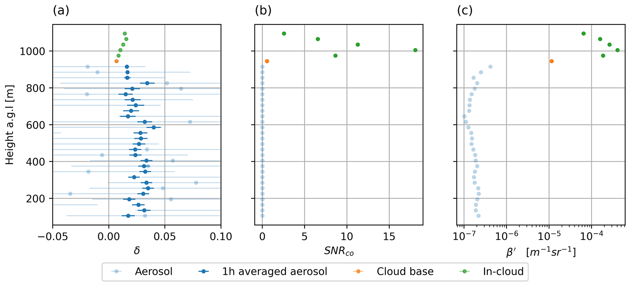
Figure 2 Atmospheric profiles observed on 24 September 2018 at 05:35:17 UTC at Hyytiälä up to 1.4 km a.g.l. (a) Depolarization ratio (δ) at the original integration time of 6 s and as 1 h average for the aerosol part of the profile. Error bar indicates the measurement uncertainty. (b) Signal-to-noise ratio in the co-polar channel (SNR_co). (c) Attenuated backscatter (β^′).

The signal from liquid cloud droplets is very strong, as seen also in Fig. 2b. Hence, there is a risk of signal saturation. Given the low bleed-through, we would expect SNR_co to get saturated before SNR_cross, which would appear as increasing δ in such cases. Figure S1 in the Supplement displays the 2D histogram of SNR_co and SNR_cross observed at liquid cloud base in Utö with the XR instrument. SNR_co and SNR_cross follow a linear relationship with the gradient corresponding to the determined bleed-through, indicating that saturation is not an issue, except maybe for some scattered points where SNR_co>6. Depending on cloud base height, the SNR_co at cloud base can be as low as 0.01. As seen in Fig. S1, there are no non-linear effects in the low SNR_co end of the spectrum, and we have no reason to suspect that the polarizer performance would deteriorate with decreasing SNR_co. We also note that previous observations with HALO Doppler lidar report near-zero depolarization ratio for marine aerosol, which we expect to be spherical and therefore have very low depolarization ratio (Vakkari et al., 2021). Therefore, we are confident that bleed-through obtained from cloud-base observations can be used to also correct weak aerosol signals.

It should be noted that at the original integration time of 6 s, the strong signal from cloud base results in a minimal noise level of δ as seen in Fig. 2a. However, for the weak aerosol signal, δ at 6 s integration time is rather noisy. Averaging over longer time periods reduces the instrumental noise in the aerosol δ substantially, as seen in the 1 h averaged δ for the aerosol part of the profile in Fig. 2a.

2.2 Aerosol identification algorithm

In order to study the seasonal pattern of the δ of aerosol, it is essential to distinguish aerosol from clouds and precipitation. For sites with a co-located cloud radar, one option would be to utilize the Cloudnet classification (Illingworth et al., 2007; Tukiainen et al., 2020), but since not all sites have full Cloudnet instrumentation (cloud radar, ceilometer, microwave radiometer), an algorithm using only Doppler lidar is required.

Using a β^′ threshold alone is not sufficient for separating aerosol and precipitation. Likewise, using a simple threshold on w alone is not sufficient for differentiating aerosol from light snowfall or precipitation from strong downdraughts. Hence, an algorithm utilizing SNR_co, β^′, and w in both the time and height domain was developed for distinguishing aerosol from larger hydrometeors.

The aerosol identification algorithm developed here utilizes 2D-kernel manipulation, which is a commonly used approach in image processing (e.g. Guo et al., 2022; Li et al., 2013; Perreault and Hébert, 2007), to extract various features from the data and to determine the correct class for each data point. A kernel, also referred to as a filter, template, window or mask (Gonzalez and Woods, 2007), is a small 2D data array. Mathematical operations, such as median, maximum, Gaussian, etc., on all values inside the kernel determine its centre value. The kernel is run through each data point one by one, replacing its centre value with mathematical operations of the neighbouring values.

Figure 3a, c and e display the measured data from the Doppler lidar in 12 August 2018 at Hyytiälä. The details of the aerosol identification algorithm are described in Sect. S3, and a brief overview is explained as follows:

1. The first step of the algorithm involves detecting potential hydrometeors and aerosols from background signals based on β^′ and SNR_co. The result of this step is shown in Fig. 3b.

2. The falling hydrometeor detection step involves separating aerosol in downdraughts due to boundary layer mixing from precipitation using both β^′ and w. Regions containing both up- and down-draughts are considered to be characteristic of boundary layer mixing, while regions of continuous downdraughts indicate precipitation. The result from this step is shown in Fig. 3d.

3. The attenuation correction step flagged all observations above clouds and precipitation with their corresponding class since the signal has been heavily attenuated. The result from this step is shown in Fig. 3f.

4. In the final step, a fine-tuned aerosol identification process is utilized to improve the aerosol class determination accuracy. First, aerosol clusters are identified using both time and height domain. Then based on the average speed of the aerosol cluster and its connectedness to the first lidar range gate, it can be classified as either aerosol, hydrometeor or undefined. The final result is shown in Fig. 3g.

The resulting classes are background signal, aerosol, hydrometeor and undefined. For this algorithm, hydrometeors are defined as cloud (liquid or ice) or precipitation (rain or snow) and do not include aerosol.

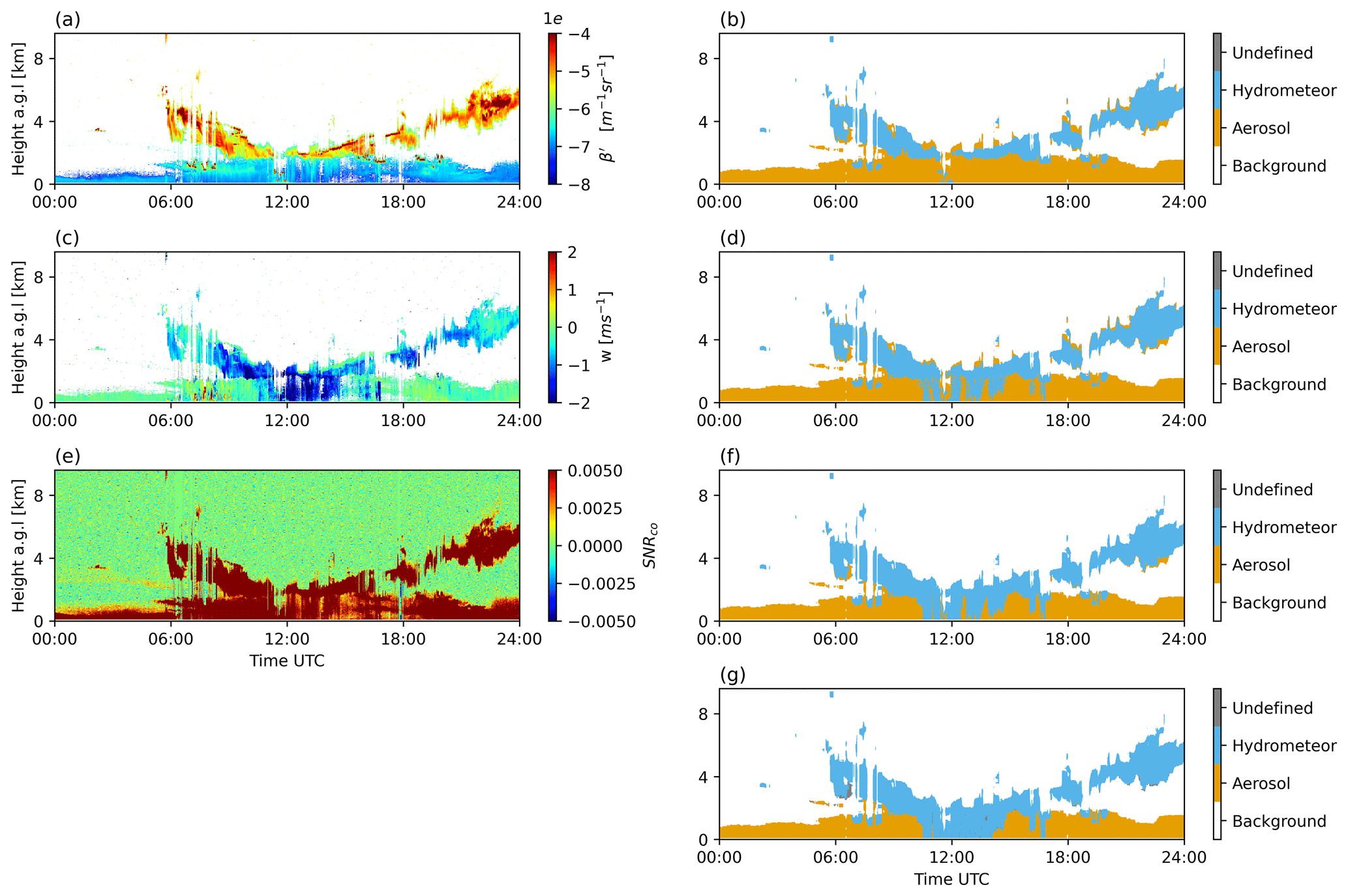
Figure 3 Atmospheric profiles on 12 of August 2018 at Hyytiälä. The left column displays the measured data where the background noise has been filtered for visualization in (a, c). (a) Attenuated backscatter (β^′); (c) vertical velocity (w); (e) signal-to-noise ratio in the co-polar channel (SNR_co). The right column displays the steps from the aerosol identification algorithm. (b) First step; (d) second step; (f) third step; (g) final step, i.e. the final result.

2.3 Post-processing

Aerosol is expected to be well-mixed within each aerosol layer, so in order to extract weak aerosol signal and minimize the random noise, SNR_co and SNR_cross were averaged for 1 h.

As mentioned before, the SNR data in this study have been processed with the background correction algorithm described by Vakkari et al. (2019). Briefly, the noise floor consists of a non-polynomial component, which is obtained from the background checks according to Vakkari et al. (2019) and a polynomial component, which is obtained from a fit to the aerosol- and hydrometeor-free (background) range gates of each SNR_co and SNR_cross profile (Manninen et al., 2016; Vakkari et al., 2019). Typically, the linear part of the noise floor is much larger than the second-order polynomial component, but for extended averaging (more than 1 h) it is essential to include in the background correction. An example of this is shown in Fig. 4a demonstrating how this second-order polynomial component can greatly affect the δ of aerosol retrieval in aerosol layers with low SNR (Fig. 4d). Previously (Vakkari et al., 2021; Bohlmann et al., 2021), the second-order component of the noise floor has been fitted to aerosol- and hydrometeor-free range gates of the SNR profiles based on visual inspection of individual profiles. However, given the large number of profiles analysed in this study, this approach is not feasible; thus, we have automated the fitting of the second-order polynomial. The fitting algorithm is described in detail in the Sect. S2, and the resulting SNR_co and SNR_cross profiles are shown in Fig. 4b and c.

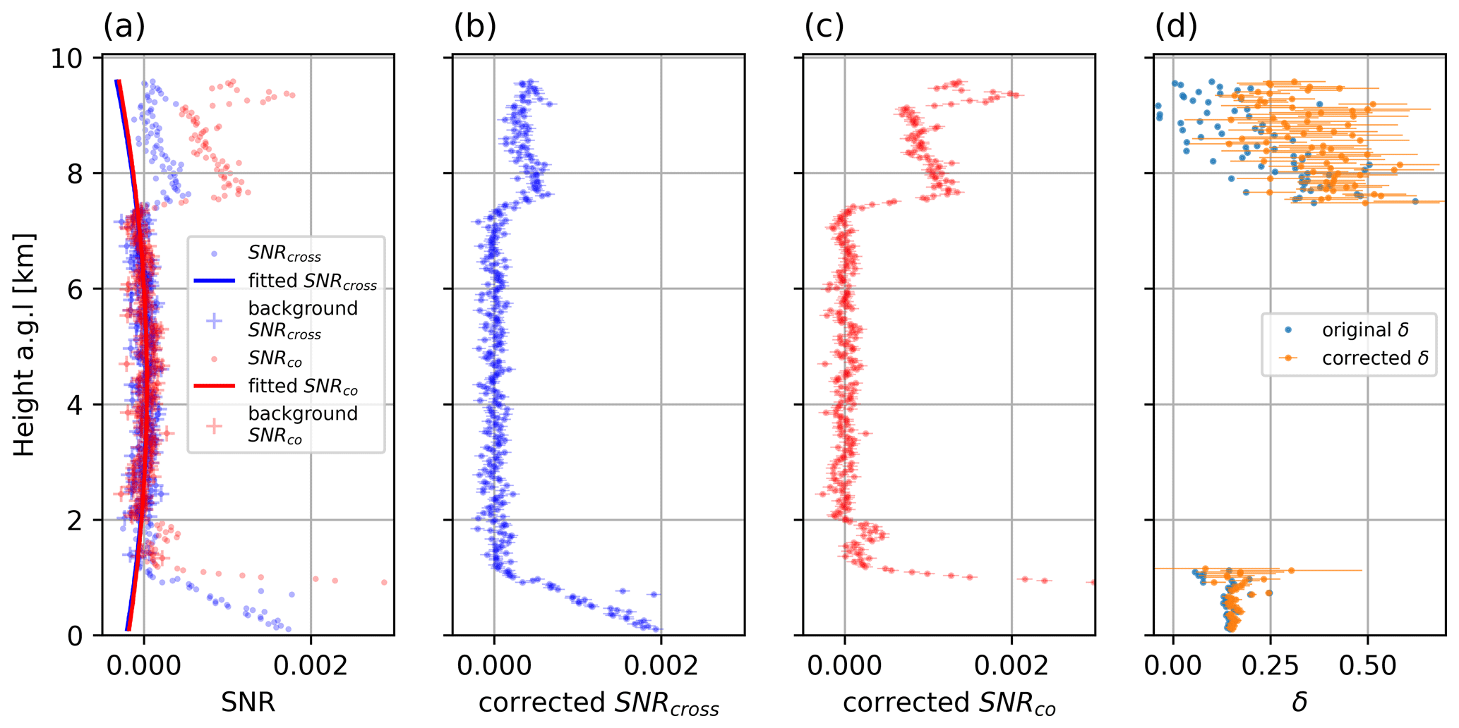
Figure 4 An example result of the post-processing procedure on 30 August 2019 at 13:00 to 14:00 UTC at Hyytiälä with instrument 46. (a) Profiles of co- and cross-polar signal-to-noise ratio (SNR_co and SNR_cross), where aerosol- and hydrometeor-free regions and the corresponding second-order polynomial fits are indicated; (b) corrected SNR_cross profile with error bar representing the fitting uncertainty; (c) corrected SNR_co profile with error bar representing the fitting uncertainty; (d) δ profile before and after the second-order fit correction.

The attenuated backscatter is calculated from the background-corrected SNR_co. Next, the aerosol layer(s) is (are) identified using the aerosol identification algorithm. Finally, following Vakkari et al. (2021), the bleed-through-corrected δ in aerosol regions is calculated as

$$\begin{array}{}\text{(3)}& \mathit{\delta }={\displaystyle \frac{{\mathrm{SNR}}_{\mathrm{cross}}-B\cdot {\mathrm{SNR}}_{\mathrm{co}}}{{\mathrm{SNR}}_{\mathrm{co}}}},\end{array}$$

where B is the estimated bleed-through of each instrument (Table 3).

The resulting δ is shown in Fig. 4d, and the estimation of its uncertainty is presented in Sect. S2. Additionally, the post-processed δ of aerosol was collected from the whole data set and compared with the original δ. The result described in Sect. S2 shows that the post-processing procedure substantially improved the δ of aerosol with low SNR values.

2.4 Air mass origin

For two case studies, the air mass origin was investigated using the Lagrangian transport model FLEXPART version 10.4 run in backwards mode (Seibert and Frank, 2004; Stohl et al., 2005; Pisso et al., 2019). FLEXPART was run using the ERA5 reanalysis obtained from the European Centre for Medium-Range Weather Forecasts (ECMWF) as the meteorological input. ERA5 was obtained with a temporal resolution of 1 h and a spatial resolution of 0.25^∘ for a domain covering 125^∘ W to 75^∘ E and 10 to 85^∘ N. Vertical model levels 50–137 were retrieved, which includes approximately the lowest 20 km a.g.l. For the elevated layers considered in the case studies, FLEXPART was run backwards in time for 7 d, and potential emission sensitivity (PES) was saved with 1 h temporal and 0.2^∘ latitude–longitude resolution. The output resolution in the vertical was 250 m from ground level to 5 km a.g.l. Above 5 km a.g.l., output levels at 10 km a.g.l. and 50 km a.g.l. were included. PES is proportional to the air mass residence time in a grid cell and was obtained in units of seconds (Seibert and Frank, 2004; Pisso et al., 2019).

3 Results and discussion

3.1 Instrumental performance

3.1.1 Noise floor level

Figure 5a displays the noise floor level for each instrument, calculated as the standard deviation of the SNR_co (σ_SNR) in the aerosol- and hydrometeor-free region. As expected, integration time is one important factor with, for example, instrument Utö-32 showing a dramatic increase in the noise floor level in summer 2016 when the integration time was decreased (from 27.5 to 5 s). Since each instrument may have its own configuration, normalization of the noise floor level considering such differences is required in order to compare the noise floor between instruments.

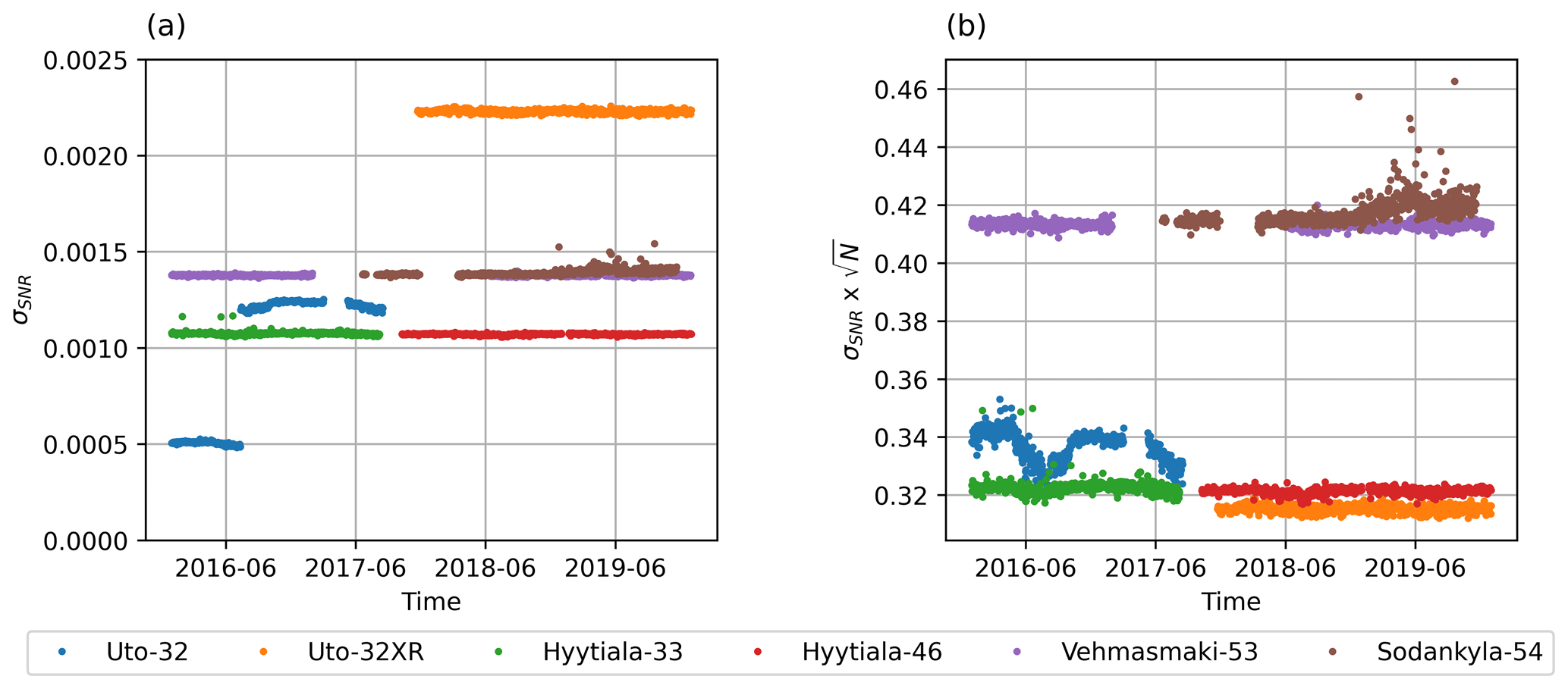
Figure 5 (a) Standard deviation of the background co-polar signal-to-noise ratio (σ_SNR). (b) The same but scaled with number of pulses in each integration (denoted with N).

Figure 5b illustrates the noise floor levels calculated after scaling for the number of pulses in each integration time and demonstrates that most instruments remained stable during the study period. Fluctuations were observed in the noise floor level for the old instrument Utö-32, but the noise floor level itself is deemed to be low, with visual inspection indicating no issues in the data quality. Sodankylä-54 is the only instrument that shows a systematic increase in the noise floor level over time. This is a worrying sign, but so far, the increase in the noise floor has been relatively small at approximately 2 % from 2017 to 2019. However, further increases in the noise floor will begin to limit the retrieval of weak signals.

The StreamLine Pro lidar instruments, Vehmasmäki-53 and Sodankylä-54, have similar and systematically higher noise floor levels than the other instruments. This is due to the fact that the Streamline Pro models were configured to utilize only half of the bandwidth, i.e. half the Nyquist velocity. Assuming the noise is thermal noise and evenly distributed across the frequency spectrum, reducing the bandwidth by half will reduce the noise power by half (Nyquist, 1928; Johnson, 1928). The Utö-32XR instrument, which is the Utö-32 system after being upgraded with a StreamLine XR transmitter and receiver, has the lowest noise floor of all instruments in this study.

3.1.2 Bleed-through

Figure 6 displays the time series and the distribution of δ at liquid cloud base for each instrument in the network. The time series is used to assess the stability of the internal polarizer over time, and the distribution is used to calculate the bleed-through (B) and its uncertainty. Overall, there is no significant trend in the bleed-through of all the instruments.

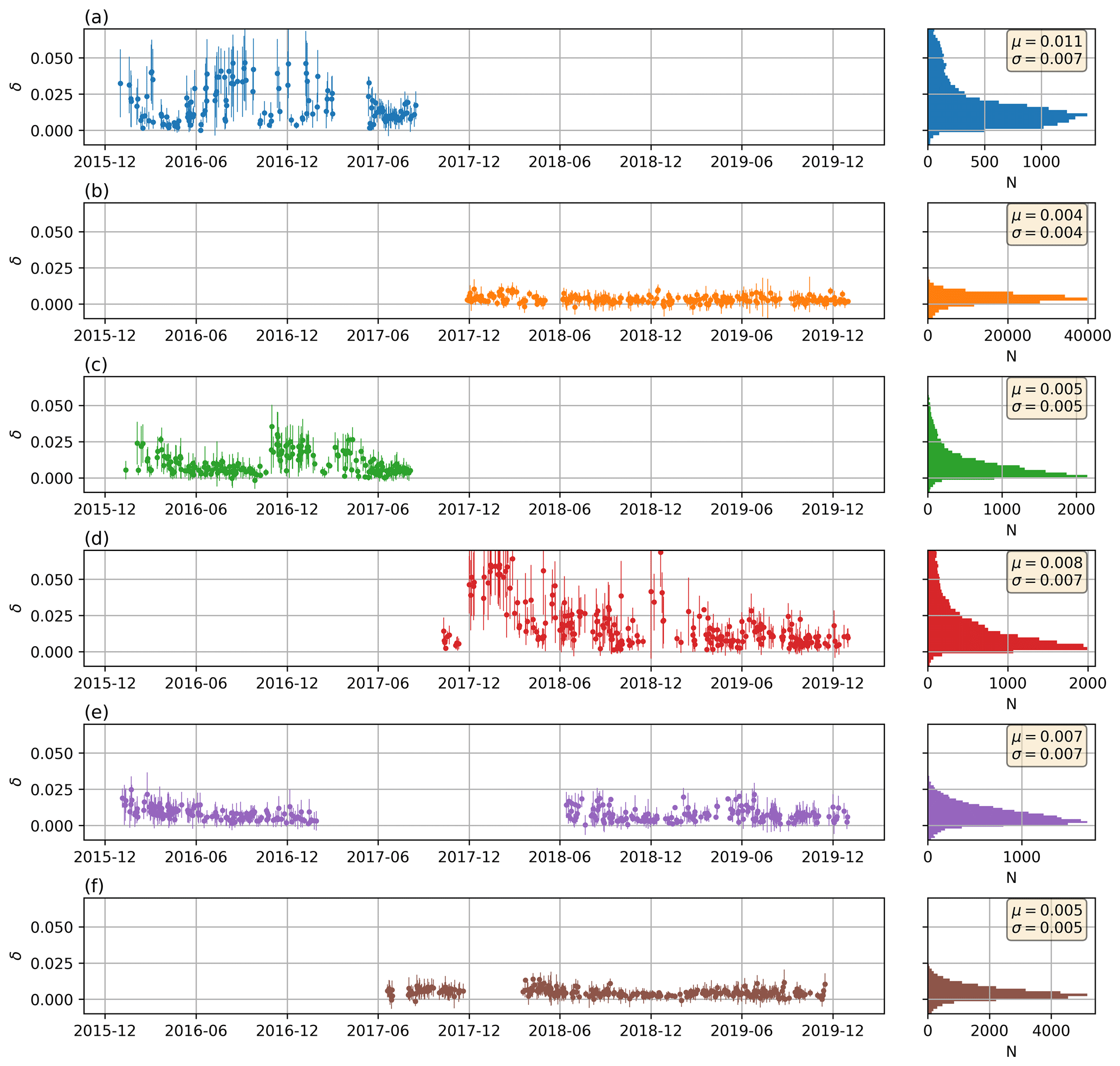
Figure 6 Time series (left panels) and histograms (right panels) of depolarization ratio (δ) at liquid cloud base in (a) Utö-32, (b) Utö-32XR, (c) Hyytiälä-33, (d) Hyytiälä-46, (e) Vehmasmäki-53 and (f) Sodankylä-54. The best estimates of mean (μ) and standard deviation (σ) of δ at the liquid cloud base in each site are shown in the right panel.

For Utö-32 (Fig. 6a), the mean bleed-through is the highest of all the instruments in this study. This probably stems from its long integration time configuration (see Table 2), resulting in SNR_co and SNR_cross not measuring the same part of the cloud. In addition, the occurrence of liquid cloud varies in time and with location. Mixed-phase clouds are difficult to distinguish from liquid-only clouds; hence, the high value of δ at liquid cloud base, especially during wintertime (Fig. 6), might be due to the misclassification with mixed-phase clouds. This effect is more prominent in Utö-32 and Hyytiälä, leading to longer-tailed distributions (Fig. 6c and d) than at other sites. On the other hand, for Utö-32XR, Vehmasmäki-53 and Sodankylä-54 (Fig. 6b, e and f), the δ at the collected liquid cloud base varies much less and remains stable at a low level (δ<0.01) throughout the year.

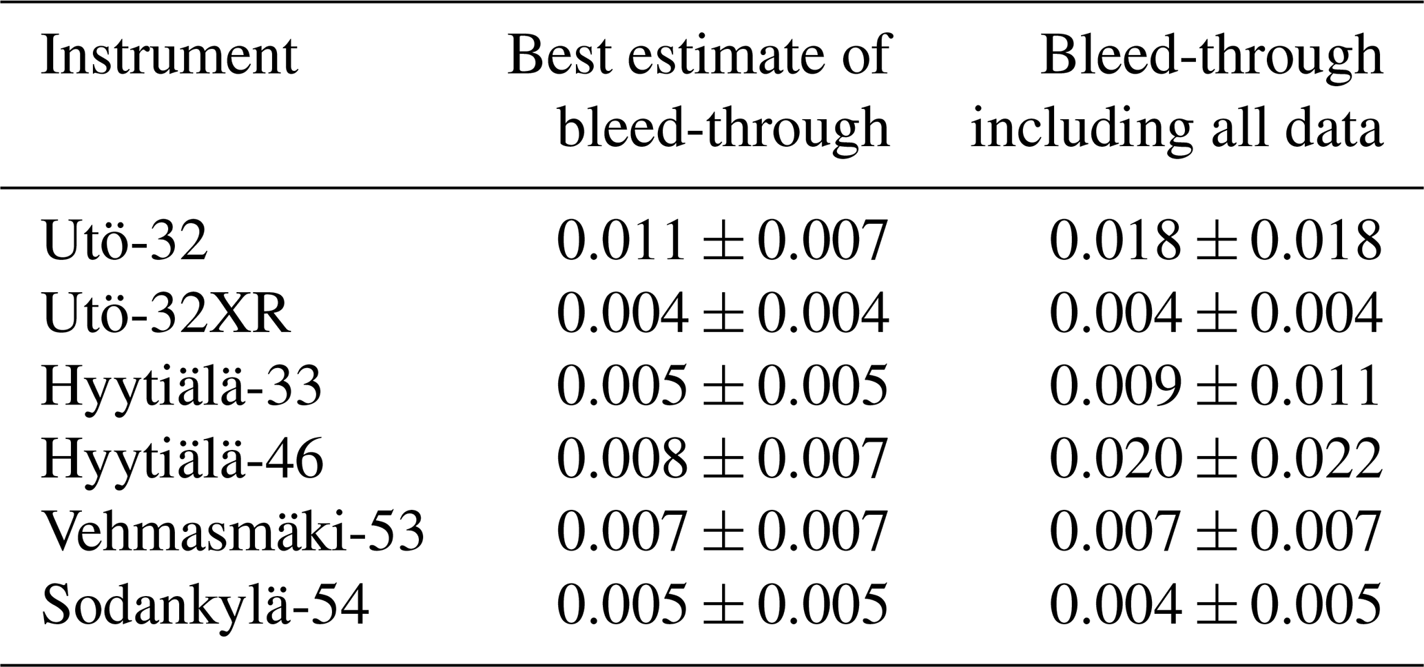
To quantify the bleed-through of the internal polarizer, the elevated value of δ due to imperfect sampling of pure liquid clouds need to be excluded. Here, we assume that for Utö-32, Hyytiälä-33 and Hyytiälä-46 the tail of the distribution is due to mixed-phase clouds or non-ideal sampling of liquid clouds, whilst the peak of the distribution is from the liquid cloud base. A Gaussian mixture model, which is a variant of finite mixture models (Baek et al., 2010), was used to derive the mean and standard deviation of δ at the liquid cloud base ignoring the tail of the distribution. For most instruments, excluding the tail of the distribution in Fig. 6 has a minimal effect on the average bleed-through estimate, which remains around 1 % as shown in Table 3. The largest effect is seen for Hyytiälä-46, where including all δ values at liquid cloud base results in a bleed-through estimate of 0.020 ± 0.022, while excluding the tail decreases the bleed-through estimate to 0.008 ± 0.007. Overall, the values of the best-estimate bleed-through in this study are smaller than the previous short case study estimates of 0.011 ± 0.007 in Limassol (Vakkari et al., 2021) or 0.016 ± 0.009 and 0.013 ± 0.006 in Vehmasmäki (Vakkari et al., 2021; Bohlmann et al., 2021) for similar instruments.

Table 3 Bleed-through (mean and standard deviation of depolarization ratio at the liquid cloud base) for each instrument.

3.2 Comparing aerosol identification algorithm with Cloudnet classification

Cloudnet's goal is to provide continuous ground-based observations of the cloud properties for forecast and climate model (Illingworth et al., 2007). On the other hand, the primary aim of the aerosol identification (AI) algorithm developed here is to exclude hydrometeors from the aerosol mask to ensure that aerosol characteristics are not biased by signal from hydrometeors.

Of all the sites in this study, only Hyytiälä belongs to Cloudnet. There, the result of the aerosol identification algorithm based on Doppler lidar only (Sect. 2.2) can be compared with the classification from Cloudnet (Illingworth et al., 2007; Tukiainen et al., 2020). However, there are marked differences between the two algorithms. The Cloudnet classification algorithm utilizes a combination of several instrument, most importantly being lidar and cloud radar (Illingworth et al., 2007). The backscattered signal from radars is much more sensitive to the diameter (D) of the particle, ∼ D⁶ (Rauber and Nesbitt, 2018), compared to lidar with only ∼ D² (Weitkamp, 2005). As a result, the radar's signal is dominated by larger particles, while the lidar is dominated by smaller particles with higher concentration. Additionally, the extinction of radar signal in non-precipitating clouds is negligible, so it can observe much further into the clouds.

Figure 7 presents a side-by-side comparison example of the results from these algorithms. At first glance, it is obvious that Cloudnet underestimates the extent of the aerosol layer compared to the aerosol identification algorithm. This is due to the improved post-processing procedure applied to the Doppler lidar data, which allows the aerosol identification algorithm to capture data from weaker aerosol signal than Cloudnet. Unsurprisingly, cloud mask in Cloudnet classification includes the full cloud layer, while the aerosol identification algorithm indicates often only the cloud base due to the attenuation of lidar signal. There are some minor differences in the precipitation zone such as right before 18:00 UTC in Fig. 7a and b and at 18:00 UTC in Fig. 7e and f, when some parts of the precipitation in Cloudnet are flagged as aerosol in the aerosol identification algorithm. This is probably due to the differences in sensitivity of different particle size in cloud radar and lidar as discussed previously. Figure 7g and h display a snow event from 00:00 to around 11:00 UTC. Cloudnet shows that some parts of snowfall eventually melt into raindrops near the ground, whilst the aerosol identification algorithm correctly classified the whole event as hydrometeor.

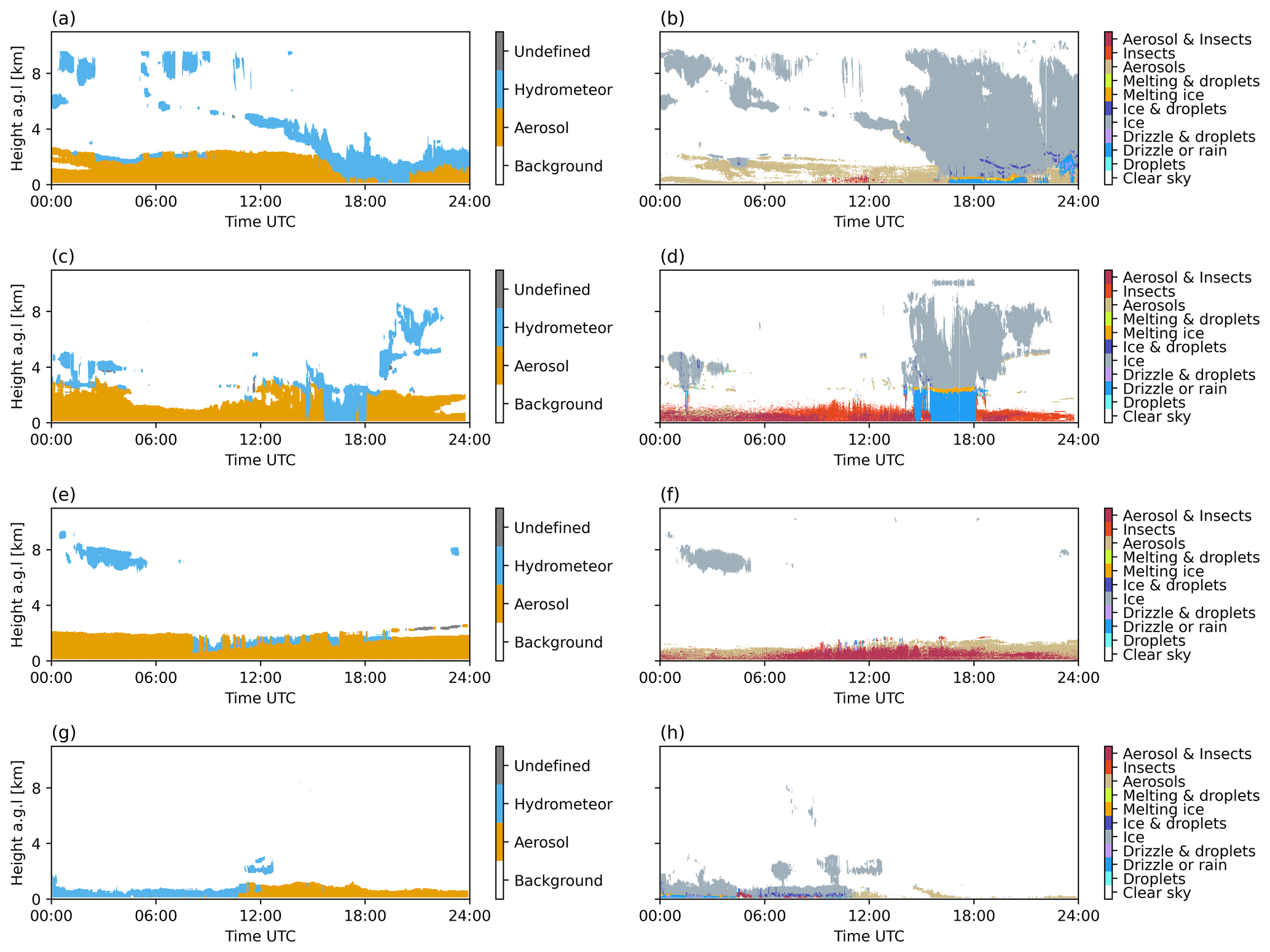
Figure 7 Results in Hyytiälä from the aerosol identification algorithm and Cloudnet classification algorithm, respectively, on (a, b) 11 June 2018; (c, d) 7 April 2019; (e, f) 7 August 2019; and (g, h) 31 December 2019.

After comparing all the data in Hyytiälä throughout the whole study period, we found that 7.7 % of the aerosol data points from the aerosol identification algorithm are classified as hydrometeor in the Cloudnet algorithm. This result shows that the aerosol identification algorithm performs adequately in extracting aerosol data compared to the Cloudnet classification algorithm. The differences between these two algorithms stem from differences in goals and instrumentation. Given the large amount of data, we are confident that the aerosol identification algorithm is capable of extracting the overall statistics of the δ of aerosol for the purpose of this study.

3.3 Aerosol particle depolarization ratio

3.3.1 Case studies

Here, we present two case studies of elevated aerosol layer observed by the lidars in southern Finland. The δ of aerosol was obtained following the post-processing procedure described in Sect. 2.3

Hyytiälä and Utö in April 2018

From late night on 14 April to morning on 15 April 2018, an elevated aerosol layer between 2 to 4 km a.g.l. was observed above Hyytiälä (Fig. 8a, b). The average profiles (Fig. 8e, f) from 03:00 to 04:00 UTC on 15 April 2018 show an elevated aerosol layer with the δ of aerosol at 0.24 ± 0.008, while in the boundary layer (from the surface to 1.5 km a.g.l.) the δ of aerosol is at 0.12 ± 0.004. Similarly, an elevated aerosol layer between 2 to 3 km was also observed in Utö (Fig. 8c, d). The averaged profiles (Fig. 8e, f) from 00:00 to 01:00 UTC on 15 April show that the δ of this layer is at 0.226 ± 0.005, while in the boundary layer (from the surface up to 2 km) the δ of aerosol is between 0.05 and 0.1. These substantial differences in the δ of aerosol between the elevated layer and the boundary layer indicate that the elevated aerosol had likely undergone long-range transport to these sites.

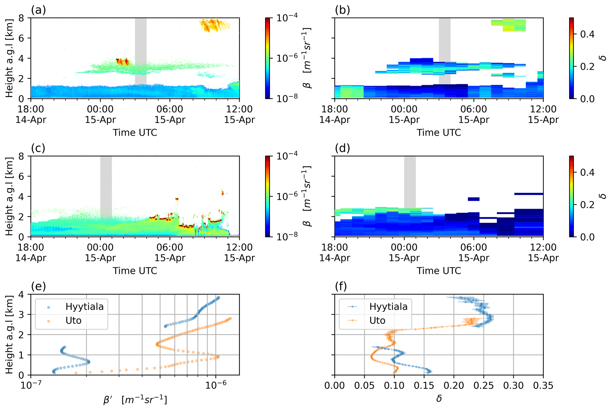
Figure 8 Profiles from 14 to 15 April in Hyytiälä and Utö. (a) Attenuated backscatter (β^′) in Hyytiälä, (b) 1 h averaged depolarization ratio (δ) in Hyytiälä, (c) attenuated backscatter (β^′) in Utö and (d) 1 h averaged depolarization ratio (δ) in Utö. And 300 m running mean (in shaded area) on 15 April 2018 03:00-04:00 UTC in Hyytiälä and 15 April 2018 00:00–01:00 UTC in Utö of (e) β^′ profiles (f) δ profiles.

The FLEXPART simulation of this layer (Fig. S5.3) indicates that the air mass was not in contact with the surface for 4.5 d prior to arrival over Hyytiälä. However, 5–7 d before arrival, a contribution from the surface layer was seen coming mostly from the western Sahara, with minor contributions from the Mediterranean. On 15 April an overpass by CALIPSO crossed the air mass transport pathway relatively close to the observation sites in Finland at 62.8^∘ N, 24.3^∘ E, and the CALIOP aerosol subtype V4.2 product indicates a dust layer at 3–5 km above ground at this location (Fig. S5). On 15 April also dust aerosol optical depth at 550 nm from the CAMS model (Benedetti et al., 2009; Morcrette et al., 2009) indicates the presence of dust over southwestern Finland (Fig. S6).

These results suggest that the layer is most likely Saharan dust, although the observed δ is slightly lower than the value of 0.30 reported by Vakkari et al. (2021) for dust at 1565 nm. This could be due to gravitational settling of large dust particles during long-range transport (Haarig et al., 2017b).

3.3.2 Utö in May 2017

On 13 May 2017, an elevated aerosol layer between 800 m a.g.l. and 2 km a.g.l. was observed over Utö (Fig. 9). For the period on 13 May 2017 from 18:00 to 20:00 UTC, the δ of this elevated aerosol layer is at 0.23 ± 0.01 and decreases with height (Fig. 9d and f). At the same time, the δ of the boundary layer aerosol from the surface up to 500 m is at 0.26 ± 0.009.

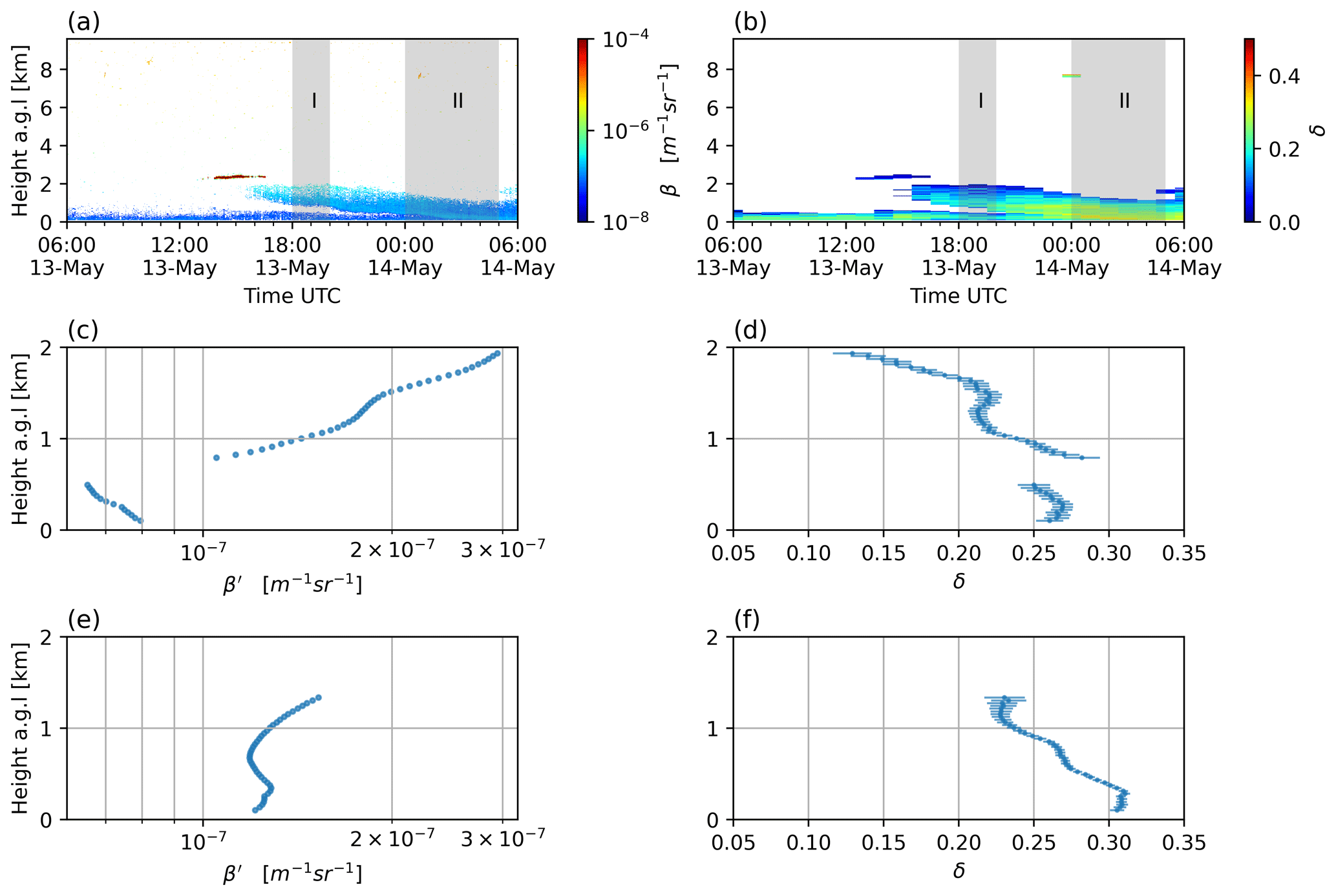
Figure 9 Profiles from 13 to 14 May 2017 at Utö; (a) attenuated backscatter (β^′); (b) 1 h averaged depolarization ratio (δ); 300 m running mean (shaded area I) at 13 May 2017 18:00–20:00 UTC of (c) the β^′ profile and (d) the δ profile. The 300 m running mean (shaded area II) during 14 May 2017 00:00–05:00 UTC of (e) the β^′ profile and (f) the δ profile.

The air mass history shows that this layer originated from both offshore in the Baltic Sea and from continental Finland (Fig. S6). The layer was elevated from the surface only 1 d before arrival and remained at a height of 1–2 km a.g.l. In this region, there are no other known sources of aerosol with such high δ except for pollen; thus, this layer is probably pollen transported from the surrounding continental areas. From 14 May 2017 00:00–05:00 UTC, this layer merged into the boundary layer, with the maximum value of δ in the boundary aerosol layer increasing to 0.30 ± 0.007. This value of δ is comparable to previous observations at the same wavelength for spruce pollen in boreal forest; 0.269 ± 0.005 (Vakkari et al., 2021) and 0.29 ± 0.10 (Bohlmann et al., 2021).

3.3.3 Long-term analysis

Here, we analyse the δ in aerosol region (δ of aerosol) from the 4-year observational data set at four sites in Finland. The δ of aerosol was obtained following the post-processing procedure described in Sect. 2.3, and the aerosol identification algorithm (Sect. 2.2) was used to exclude hydrometeors from the data set. All data that have standard deviation of the δ of aerosol larger than 0.05 have been filtered out.

Table 4 Overall statistics of δ_aerosol across all the sites.

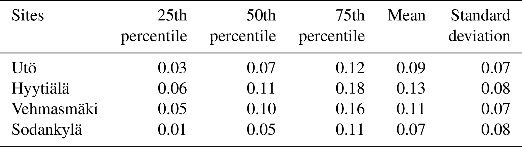
Overall, as seen in Table 4, the average δ of aerosol is higher in the boreal forest sites of Hyytiälä (0.13 ± 0.08) and Vehmasmäki (0.11 ± 0.07) compared to Utö (0.09 ± 0.07) and Sodankylä (0.07 ± 0.08). This can be explained by the abundance of pollen with high δ in the boreal forest sites (Aaltonen et al., 2012; Shang et al., 2020; Vakkari et al., 2021; Bohlmann et al., 2021). Located in the marine site, the lidar at Utö observes a high fraction of marine aerosols with low δ, as also found in previous studies (Groß et al., 2011, 2013; Haarig et al., 2017a; Vakkari et al., 2021; Mylonaki et al., 2021). In Sodankylä, which is a clean rural sub-arctic environment, the δ of aerosol is found to be the lowest of the sites considered here.

Figure 10 shows the average monthly median of the δ of aerosol for all sites. Overall, the δ of aerosol is increased in the summer and remains low in the winter. The enhanced values of the δ of aerosol from April to the end of September coincide with the growing season of the boreal forest (Manninen et al., 2014), when airborne pollen and other particles of biological origin are abundant in Finland. The most common sources of pollen in the Finnish boreal forest are birch (Betula), spruce (Picea), pine (Pinus) and nettle (Urtica). They contribute to more than 90 % of the total pollen load (Shang et al., 2020; Manninen et al., 2014). The peaks of the δ of aerosol occurs in the pollen season of birch, spruce, and pine (Shang et al., 2020) between May and early June. The irregular shape of these pollen types has been observed to have high δ such as 0.10 ± 0.06 for birch at 532 nm (Bohlmann et al., 2019), 0.29 ± 0.10 for spruce at 1565 nm (Bohlmann et al., 2021) and 0.36 ± 0.01 for pine at 532 nm (Shang et al., 2020). The relatively high concentration of these pollen grains in the atmosphere likely explains the peak of the δ of aerosol in May for the boreal forest sites of Hyytiälä and Vehmasmäki.

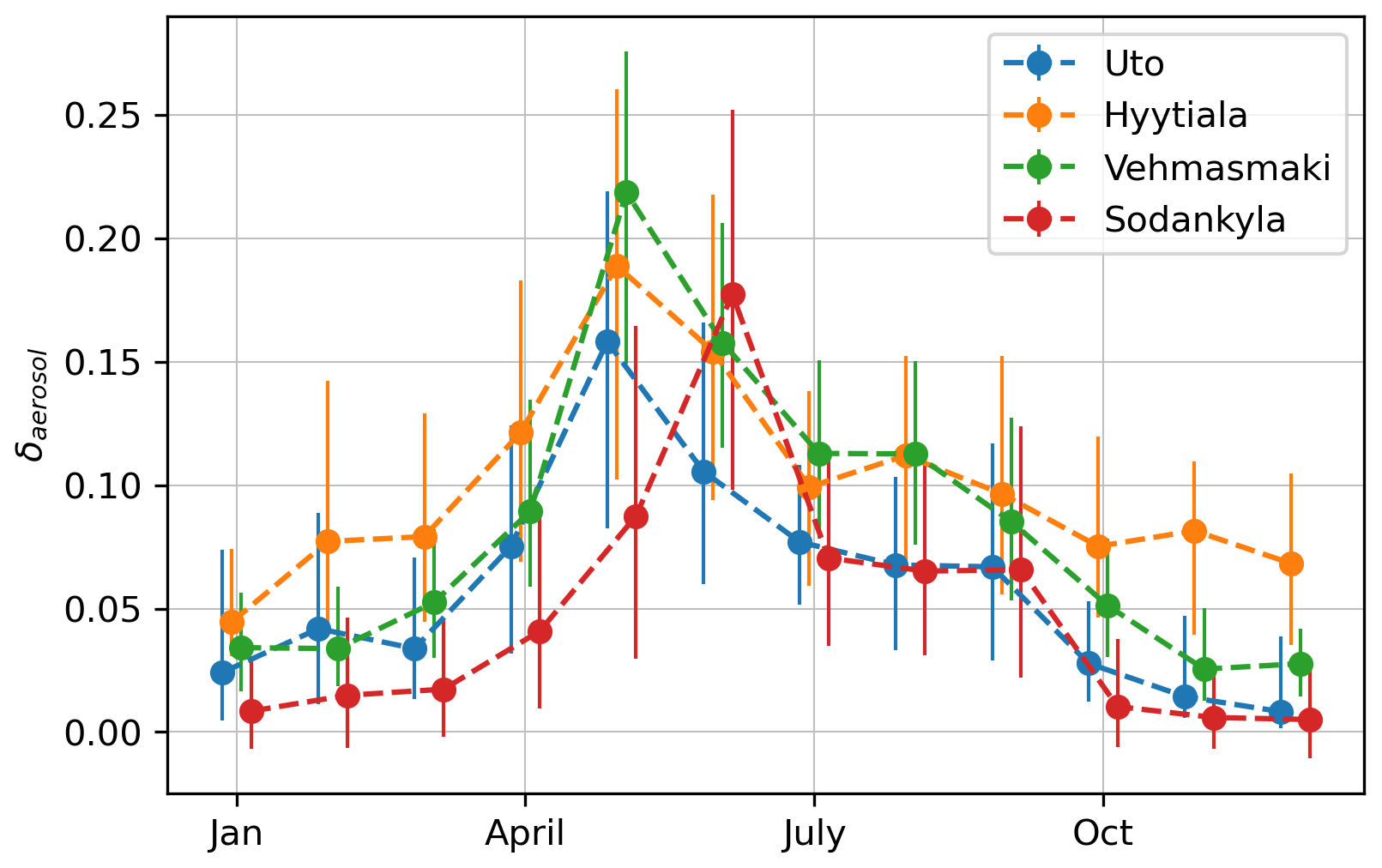
Figure 10 Monthly median of the particle depolarization ratio of aerosol (δ_aerosol) across all the sites; error bars show the 25th and 75th quantile.

However, the peak in the δ of aerosol at Sodankylä occurs 1 month later than the other sites. Due to its location in the sub-arctic, the snowmelt and the beginning of the pollen season start later around June in Sodankylä than at other sites in central and southern Finland (Koivikko et al., 1986; Oikonen et al., 2005). Interestingly, despite its marine location, the δ of aerosol in Utö also peaks in May, and the δ of aerosol value remains high during summer, probably due to transported pollen from the mainland. Even though pollen grains are typically large from 10 to 100 µm (Manninen et al., 2014), they are low-density particles, which make them prone to be lifted by turbulent air flows up to several kilometres and be dispersed by the wind (Bohlmann et al., 2019). Several studies (Rousseau et al., 2003, 2006; Skjøth et al., 2007; Szczepanek et al., 2017) have demonstrated the long-range transport of pollen over thousands of kilometres. Additionally, marine aerosol at lower relative humidity in the summer (see Fig. 12) could contribute to the higher δ of aerosol in the summer at Utö. Haarig et al. (2017a) found that at low relative humidity, elevated marine aerosol can crystalize and become mostly cubic-like in shape (Wise et al., 2007), which results in a higher δ of aerosol up to 0.15 ± 0.03 at 532 nm and 0.1 ± 0.01 at 1064 nm.

During the winter months from October to March, the δ of aerosol remains low across all sites. Luoma et al. (2019) found that there is a high fraction of aerosol from anthropogenic sources and domestic wood burning in the winter in Hyytiälä, and these are probably major sources of aerosol in other continental sites as well. Burton et al. (2015) reported the δ of smoke as 0.019 ± 0.005 at 1064 nm, and with its negative wavelength dependency (Haarig et al., 2018; Ohneiser et al., 2020), the δ of smoke at 1565nm would probably have even smaller values. Anthropogenic aerosol has also been found to have small δ values < 0.05 at 532 nm (Müller et al., 2007; Burton et al., 2013; Mylonaki et al., 2021). The low δ of aerosol in Utö < 0.05 agrees with the typical δ of wet and polluted marine aerosol found at various wavelengths (Groß et al., 2011; Haarig et al., 2017a; Vakkari et al., 2021; Mylonaki et al., 2021).

Figure 11a, b, c and d display the average δ of aerosol as a function of height for each site. During summer from April to August, aerosols with high δ are concentrated within the boundary layer, often below 1 km a.g.l. However, in Vehmasmäki during May, the δ of aerosol increases with height, it can reach up to 0.3 at 1.2 km a.g.l. As mentioned, pollen grains can get easily lofted to higher altitude and since the air is dryer at high altitude, pollen might fold onto itself to prevent further dehydration which would lead to higher δ (Bohlmann et al., 2019).

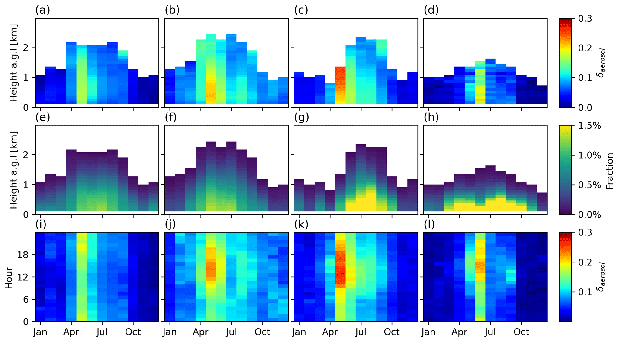
Figure 11 Median of the particle depolarization ratio of aerosol (δ_aerosol) profiles across all the sites. Utö (a, e, i); Hyytiälä (b, f, j); Vehmasmäki (c, g, k); Sodankylä (d, h, l). Distribution of δ_aerosol with height in each month is shown on the first row (a, b, c, d). The frequency of observations relative to height in each month is shown on the second row (e, f, g, h). The last row (i, j, k, l) displays the diurnal pattern of δ_aerosol in each month.

In September at Utö, Hyytiälä and Vehmasmäki, aerosol with δ>0.1 can be observed at around 2 km a.g.l. This is probably due to transported aerosol since the δ of aerosol is much higher than boundary layer aerosol near the ground. During winter months from October to March, the δ of aerosol distributed uniformly at all heights for every site.

Figure 11e, f, g and h show the frequency of aerosol detected at each height level across all the sites. Overall, more aerosol is observed in the summer months and at higher altitude, due to the higher boundary layer height in summer. In Sodankylä, aerosol is observed less frequently at altitudes above 1 km a.g.l. compared to other sites.

Figure 11i, j, k and l illustrate the diurnal pattern of the δ of aerosol across all the sites. During May–June, when the monthly δ of aerosol is at its highest, the median hourly δ of aerosol in Hyytiälä, Vehmasmäki and Sodankylä peaks in the afternoon. The release of pollen is positively influenced by higher temperature (Bartková-Ščevková, 2003), so the higher δ of aerosol during daytime might be due to a higher fraction of irregular-shaped pollen being released at noon. Simultaneously, higher mixing layer height during afternoon hours enables more pollen grains released at the surface to be lifted above the lidar's minimum range of 90 m (see Table 2). This result also agrees with the previous findings (Noh et al., 2013a; Bohlmann et al., 2021), where the high δ from pollen is only observed in the boundary layer during daytime.

On the contrary, during May in Utö, the δ of aerosol peaks at night and remains low during the day (Fig. 11i). We attribute this high δ of aerosol value to the transported pollen arriving from the continent at night, which may be part of the returning flow of a sea breeze circulation in the Baltic Sea (Dailidė et al., 2022).

3.3.4 The effect of relative humidity

Studies show that relative humidity (RH) can change the shape of marine aerosol (Granados-Muñoz et al., 2015; Haarig et al., 2017a) and pollen grains (Franchi et al., 1984; Katifori et al., 2010; Griffiths et al., 2012) through hygroscopic growth or rupture into smaller fragments (Taylor et al., 2002, 2004; Miguel et al., 2006; Hughes et al., 2020; Bohlmann et al., 2021). Hence, the δ of aerosol at the sites in this study may also respond to the ambient RH. However, as RH profiles are not measured, we investigate the connection between the surface RH at 2 m a.g.l. and the δ of aerosol below 300 m a.g.l.

Figure 12 shows the seasonal and diurnal pattern of the δ of aerosol and RH below 300 m a.g.l. The δ of aerosol pattern of the closest 300 m (Fig. 12e, f, g and h) is similar to that of the whole profile (Fig. 11i, j, k, l); that is, its value is highest in the summer and lowest in winter. During May and June, the continental sites present a strong diurnal variation in both RH and the δ of aerosol. However, the island of Utö also shows a similar if less pronounced diurnal cycle in RH to the continental sites but an opposite diurnal cycle response for the δ of aerosol as noted before due to transported pollen.

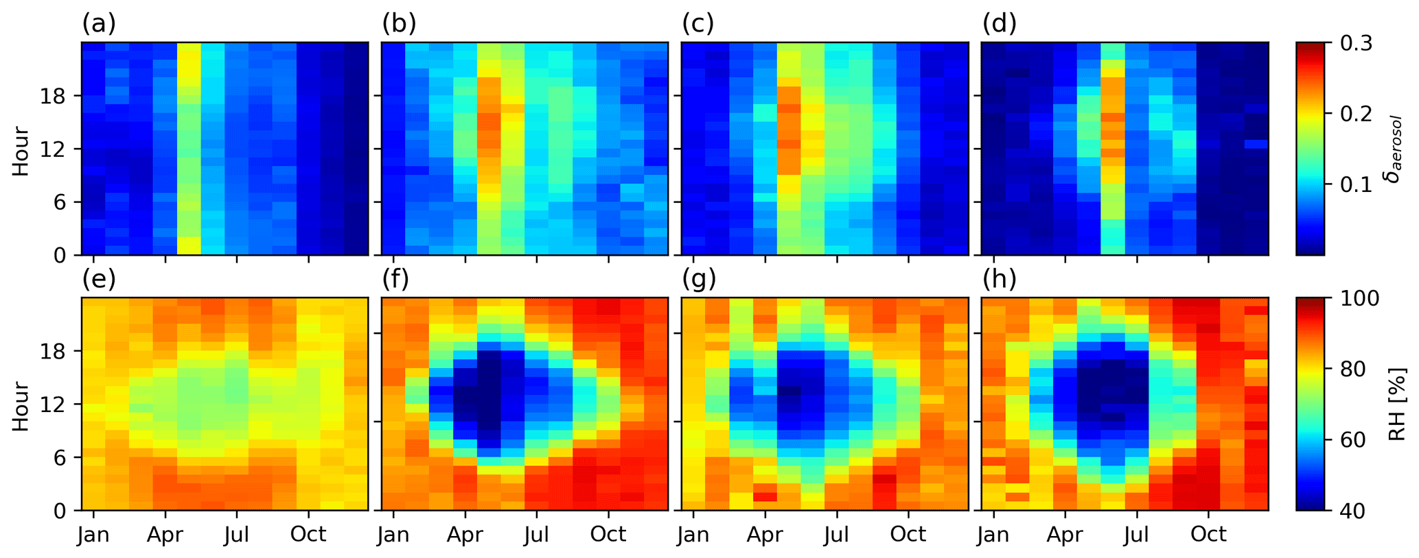
Figure 12 Diurnal pattern of aerosol depolarization ratio (δ_aerosol) from 90 m to 300 m a.g.l. and relative humidity (RH) at 2 m a.g.l., respectively, in Utö (a, e), Hyytiälä (b, f), Vehmasmäki (c, g) and Sodankylä (d, h).

Previously, pollen concentrations have been shown to be enhanced around noon when RH is at its lowest (Käpylä, 1984; Latorre and Caccavari, 2009; Noh et al., 2013b). In fact, pollen release is highly dependent on the particular ambient weather conditions including rainfall, air temperature, RH, duration of sunshine and wind speed (Gilissen, 1977; Käpylä, 1984; Jato et al., 2000; Alba et al., 2000; Adams-Groom et al., 2002; Bartková-Ščevková, 2003; Vázquez et al., 2003; Noh et al., 2013b). Moreover, low RH could affect the diffusion of pollen in the atmosphere by decreasing the specific gravity of pollen grains, thus negatively reducing their ability to settle to the ground (Durham, 1943), i.e. be more easily diffused above the lidar minimum range of 90 m a.g.l.

Statistical analysis (Table S4) shows an overall negative correlation between RH and the δ of aerosol. However, without additional data, attributing the change of aerosol physical properties (such as hygroscopic growth) as the reason for this negative correlation is not possible. The change of aerosol type such as from pollen in the summer to anthropogenic aerosol in the winter, or diurnal changes in pollen release could be the main driver of the δ of aerosol.

4 Conclusions

In this study, the use of HALO Doppler lidars for long-term monitoring of the δ of aerosol was investigated with a 4-year-long data set from the Finnish remote sensing network. The first aim was to investigate the stability of the instrumental noise floor and internal polarizer performance. The second aim was to characterize the seasonal and diurnal variation of the δ of aerosol at a wavelength of 1565 nm at four different sites in Finland. In order to facilitate the second aim, an aerosol identification algorithm was created utilizing only data from HALO Doppler lidars.

The instrumental noise floor was assessed through the time series of the standard deviation of SNR_co in noise-only (aerosol- and hydrometeor-free) conditions. Four of the six systems included in this study presented a very stable noise floor, but two systems had up to 6 % variability in the σ_SNR time series, even after changes in the configured integration time were taken into account. However, visual inspection did not indicate major issues in the data from the systems with increased variability in σ_SNR.

The time series of δ at liquid cloud base did not indicate long-term changes in the bleed-through of the HALO Doppler lidar internal polarizer. Overall, the observed values were comparable to previous case studies, though some elevated (δ>0.02) values were observed especially during the wintertime, possibly due to the inclusion of some mixed-phase clouds erroneously classified as liquid-only. Also, the configuration with very long integration time of 27.5 s resulted more frequently in elevated δ at liquid cloud base, leading to a long tail in the otherwise Gaussian distribution of δ. Excluding the tail of the distribution resulted in bleed-through estimates that are very similar for all five instruments that were included in the study, ranging from 0.004 to 0.011. Including all the δ values would increase the bleed-through estimate at most from 0.008 ± 0.007 to 0.020 ± 0.022 for the Hyytiälä-46 lidar; for other systems the effect is smaller.

Two cases of elevated, long-range-transported aerosol were studied in more detail. From late night 14 April to the morning 15 April 2018, an elevated aerosol layer between 2 to 4 km a.g.l. was observed at Hyytiälä. The unusually high δ of aerosol of 0.24 ± 0.008 for April at Hyytiälä for this event, together with aerosol subtype from CALIOP, dust aerosol optical depth from CAMS and air mass history analysis from FLEXPART indicate that this layer could be identified as Saharan dust. The δ value of this aerosol layer is comparable to previous observations of long-range-transported Saharan dust (Freudenthaler et al., 2009; Groß et al., 2011; Burton et al., 2015; Haarig et al., 2017b; Vakkari et al., 2021). On 13 May 2017 in Utö, an elevated aerosol layer with high δ was observed between 800 m and 2 km a.g.l. The air mass footprint of this layer was from the Baltic Sea and surrounding areas, suggesting the layer contained pollen originating from continental areas and arriving at Utö at night. During this episode, the δ of aerosol ranged from 0.23 to 0.30, which was well within the range of previous reports for pollen in Finland (Bohlmann et al., 2019, 2021; Shang et al., 2020; Vakkari et al., 2021).

From the 4-year observations of the δ of aerosol, we found that it is surprisingly similar at all four sites in Finland. The overall δ values of aerosol are 0.13 ± 0.08 in Hyytiälä, 0.11 ± 0.07 in Vehmasmäki, 0.09 ± 0.07 in Utö and 0.07 ± 0.08 in Sodankylä. All these sites have low values of δ of aerosol in the winter months and higher values in the summer months, which is attributed to the presence of irregular-shaped pollen particles in relatively clean background air. The highest monthly averages in the δ of aerosol are observed in May and June. During this period, the δ of aerosol has a strong diurnal cycle: at Hyytiälä, Vehmasmäki and Sodankylä, it peaks in the afternoon, while at Utö the peak is several hours later in the night. This difference for the island station of Utö is attributed to the time lag required for pollen to be transported from the mainland to the island. Additionally, the δ of aerosol in the nearest 300 m a.g.l. was found to have a negative correlation with relative humidity at the surface. However, this negative correlation could stem from either hygroscopic growth or from concurrent changes in the aerosol type, e.g. due to pollen release diurnal cycle. Attributing which factor plays a more dominant role is challenging and would require more profiling measurements.

In conclusion, the long-term performance of HALO Doppler lidars was found to be satisfactory for the determination of the δ of aerosol for continuous-monitoring purposes. Furthermore, the aerosol identification algorithm developed for this study, which is based on Doppler lidar only, was found to agree with the aerosol mask from the multi-instrument Cloudnet classification algorithm for more than 90 % of the time. This extends the capabilities of the Finnish remote sensing network (Hirsikko et al., 2014) in identifying potentially hazardous aerosol particles, which was one of the motivations in choosing HALO Doppler lidars for the network.