High-resolution temperature profiling in the Π Chamber: variability of statistical properties of temperature fluctuations

This study delves into the small-scale temperature structure inside the turbulent convection Π Chamber under three temperature differences (10, 15, and 20 K) at Rayleigh number Ra∼10⁹ and Prandtl number Pr≈0.7. We performed high-frequency measurements (2 kHz) with the UltraFast Thermometer (UFT) at selected points along the vertical axis. The miniaturized design of the sensor with a resistive platinum-coated tungsten wire, 2.5 µm thick and 3 mm long, mounted on a miniature wire probe, allowed for vertically undisturbed temperature profiling through the chamber's depth spanning from 8 cm above the bottom to 5 cm below the top. The collected data, consisting of 19 and 3 min time series, were used to investigate the variability of the temperature field within the chamber, aiming to better address scientific questions related to its primary objective: understanding small-scale aerosol–cloud interactions. The analyses reveal substantial variability in both variance and skewness of temperature distributions near the top and bottom plates and in the bulk (central) region, which were linked to local thermal plume dynamics. We also identified three spectral regimes termed “inertial range” (slopes of $\sim -\mathrm{7}/\mathrm{5}$), “transition range” (slopes of $\sim -\mathrm{3}$), and “dissipative range”, characterized by slopes of $\sim -\mathrm{7}$. Furthermore, the analysis showed a power law relationship between the periodicity of large-scale circulation (LSC) and the temperature difference. Notably, the experimental results are in good agreement with direct numerical simulation (DNS) conducted under similar thermodynamic conditions, illustrating a comparative analysis of this nature.

1 Introduction

The convection-cloud chamber, officially named the Π Chamber, represents one of the most advanced facilities for controlled experiments on cloud microphysics (Chang et al., 2016). Its design allows for reproducible and controlled measurements across a wide range of temporal scales, from minutes to days, while maintaining stationary thermodynamic forcing. It operates in two modes. The first mode utilizes static pressure reduction to simulate updrafts in the atmosphere. In the second mode, it induces Rayleigh–Bénard convection (RBC), where air in the chamber is heated from below and cooled from above. In the present study we investigate temperature fluctuations in the full spectrum of scales in the chamber operating in the second mode. We focus on small-scale temperature fluctuations in a course of turbulent mixing inside the chamber, since the facility is designed for research on aerosol–cloud interactions in turbulent environments (Chandrakar et al., 2018a, b, 2020; Desai et al., 2018, 2019; Prabhakaran et al., 2020; MacMillan et al., 2022). Unlike typical RBC experiments, the chamber includes side windows and various mounting points for microphysical instrumentation, which introduce asymmetries between the upper and lower plates. Thus, detailed (e.g., thermal) characterization of the chamber is required to evaluate how closely the flow resembles classic RBC flows. It is important to note that this study does not aim to extend beyond conventional RBC research, which often involves 1 d averaging.

Atmospheric phenomena undergo nonstationary and unstable processes, making them difficult to study under real atmospheric conditions. The RBC setup used in this study provides a more controllable environment than the real atmosphere, but we do not push to reach the level of convergence recognized in the RB community. Nonetheless, we report statistics which can be compared to previous highly resolved measurements within the RBC systems (du Puits et al., 2013; du Puits, 2022, 2024).

Our work focuses primarily on understanding the small-scale and short-term variability of thermal conditions within the facility, emphasizing the importance of absolute temperature. This aspect is crucial for more comprehensive studies on aerosol interactions with water vapor and droplet growth or evaporation in a turbulent environment. However, a few selected results are presented in a non-dimensional form (see Appendix B). One recent study of particular relevance to small-scale variability is the paper by Salesky et al. (2024) on the subgrid-scale scalar variance modeled in large-eddy simulations over the range Ra∼10⁸–10⁹. Our approach was to collect high-resolution (2 kHz) temperature time series using the UltraFast Thermometer (UFT) at selected locations in a vertical profile near the axis of the chamber and to perform statistical and spectral analyses investigating small-scale structure of RBC under laboratory conditions.

The UFT was specifically designed for airborne in-cloud measurements. It resolves scales down to or even below 1 cm, effectively reaching the dissipation range. Successive models of the UFT family (Haman et al., 1997, 2001; Kumala et al., 2013) have utilized a similar sensing element – a resistive platinum-coated tungsten wire, 2.5 µm thick and 5 mm long, mounted on a small vane to adapt to local airflow. In the next sensor versions (Nowak et al., 2018; Siebert et al., 2021), the vane was removed, leading to further miniaturization of the instrument's dimensions and the implementation of a custom-built electronic system. The current iteration (UFT-2B) underwent testing during the recent EUREC⁴A campaign (Stevens et al., 2021). The 3 mm sensing wire is spanned on an industry-standard miniature wire probe, allowing for easy exchange of the sensing head (see Fig. 1).

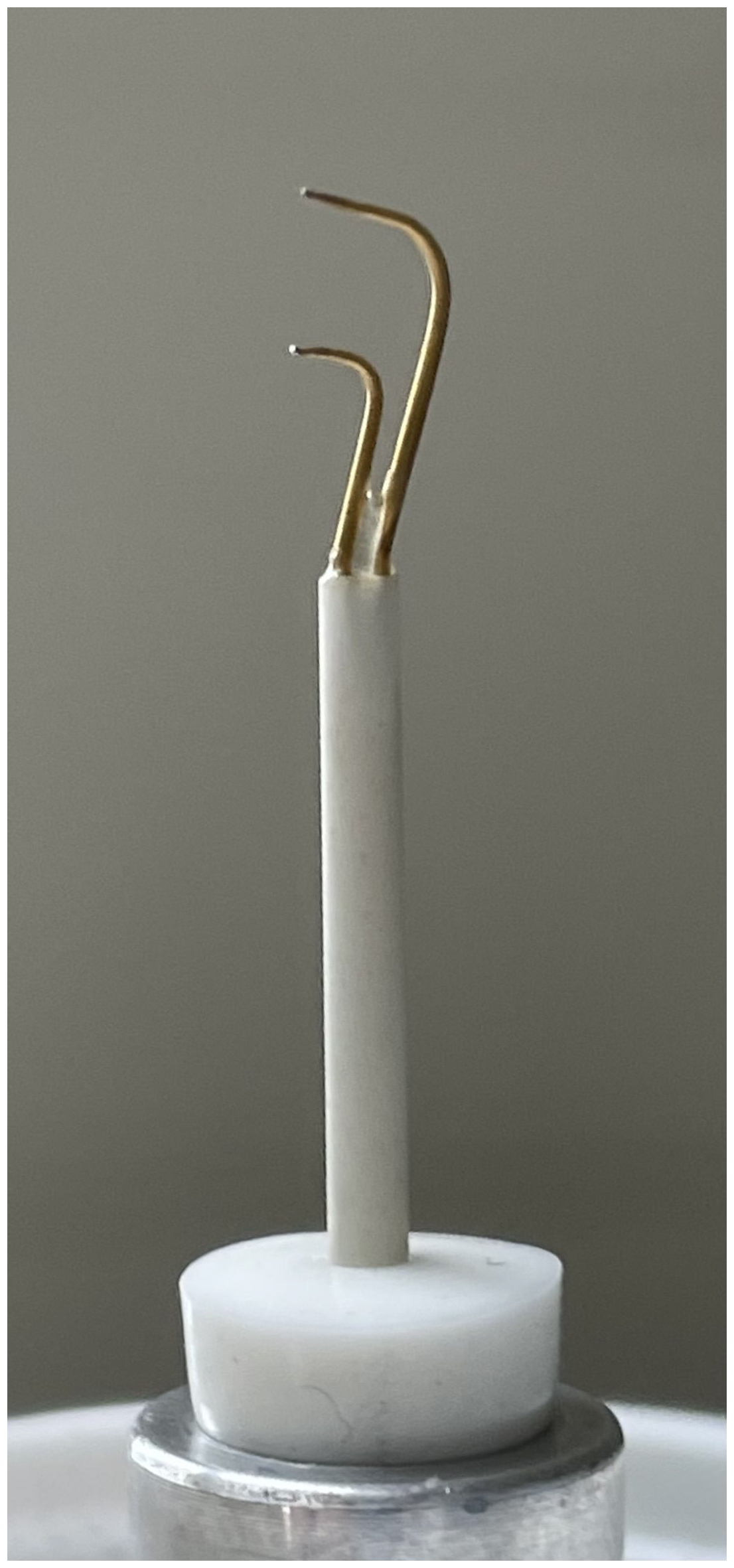
Figure 1 UFT-2B head sensor. Parallel to the mean flow, tungsten wire (2.5 µm thick, 3 mm long) spanned a miniature industry standard wire probe by DANTEC^®.

Small-scale fluctuations are important not only in their own right; they are also important for understanding changes in the large-scale circulation (LSC) of distributions of the mixing ratio, temperature, and supersaturation inside the cell. The established LSC period in the Π Chamber at a temperature difference of 12 K was estimated to be τ₁₂≈72 s (moist convection characterized by a mixing ratio of 7.55 g kg⁻¹) (Anderson et al., 2021). In this paper we investigate LSC for three temperature differences (ΔT) 10, 15, and 20 K, showing a variability of periodicity which can be described by the power law function.

To place our measurements in a broader context, we discuss the results from canonical RBC systems that have been conducted over the years. For comprehensive overviews of recent advancements in RBC, see the works by Fan et al. (2021) and Lohse and Shishkina (2024), along with their references. More detailed analyses of statistical properties of the temperature field in RBC have been explored in recent experimental (He et al., 2018; Wang et al., 2019, 2022), theoretical (Shishkina et al., 2017; Olsthoorn, 2023), and numerical (Xu et al., 2021b) studies where the authors characterized boundary layers and mixing zones of convective flows. Some investigations aimed at describing buoyant thermal plumes departing from the thermal boundary layer, contributing to the overall heat flux through LSC in a wide range of Rayleigh numbers (Ra ranging from 10⁷ to 10¹⁴) (Liu and Ecke, 2011; van der Poel et al., 2015; Zhu et al., 2018; Blass et al., 2021; Reiter et al., 2021; Vishnu et al., 2022; Wang et al., 2022). Large-scale convective structures have been explored further through direct numerical simulation (DNS), revealing relatively fewer plumes near the side walls carrying large heat fluxes, in contrast to more numerous plumes near the cell axis but with weaker heat fluxes, highlighting strong intermittency in this region (Lakkaraju et al., 2012; Chillà and Schumacher, 2012; Stevens et al., 2018; Pandey et al., 2018; Krug et al., 2020; Moller et al., 2021). The simulations also demonstrated the persistence of discrete thermal structures in RBC (Sakievich et al., 2016).

The studies also examined the effects of cell dimensions, revealing the variable nature of the LSC, depending on the cell's aspect ratio (Γ = $\text{width}/\text{height}$) (Shishkina, 2021). The aspect ratio characterizing the facility (width = 2 m, height = 1 m, and Γ = 2) corresponds to a single roll with a fixed orientation and pronounced oscillations about the mean position, a result of asymmetries inside the chamber (Anderson et al., 2021) (see Fig. 2). In cases where Γ ≳ 4, a 3D multi-roll structure has been observed (Bailon-Cuba et al., 2010; Ahlers et al., 2022). Another aspect is the stability of the LSC as numerous analyses have proven its random reorientation and reversal in both cylindrical setups (Brown and Ahlers, 2007; Mishra et al., 2011; Wei, 2021; Xu et al., 2021a) and rectangular cells (Vasiliev et al., 2016; Foroozani et al., 2017; Wang et al., 2018; Vishnu et al., 2020), without clearly indicating a superior choice.

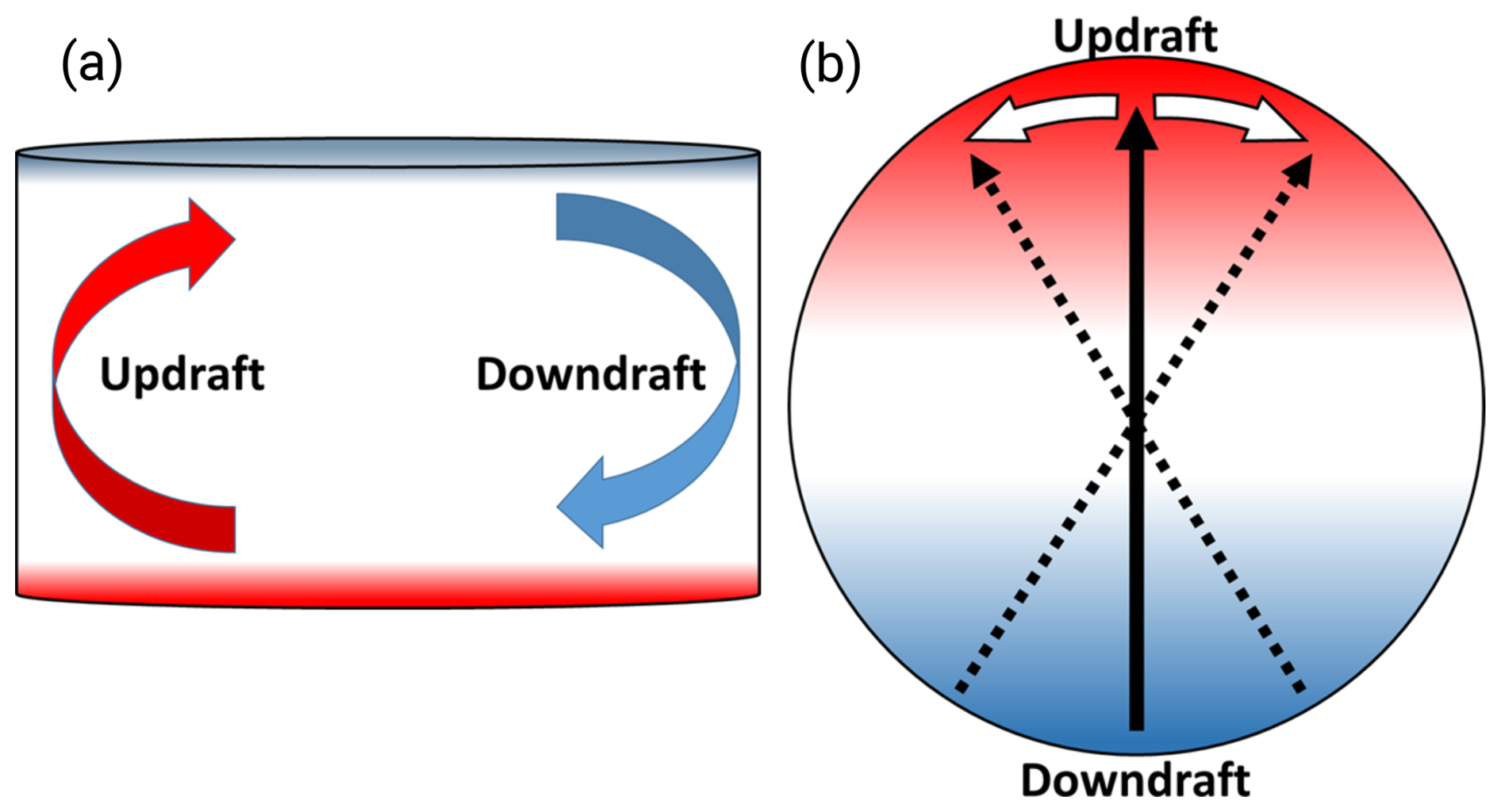
Figure 2 Schematic of the Π Chamber (a) and its plan view (b) with the marked LSC. (a) The arrows represent the mean direction of the warm updraft (red) and the cool downdraft (blue). (b) The dotted and white arrows show the azimuthal oscillations in the circulation. Figure from Anderson et al. (2021).

Natural convection plays a crucial role in heat and mass transfer within the atmosphere. Despite its fundamental importance, several aspects of this phenomenon remain poorly understood, even at a simplified level of controlled RBC conditions, and require further investigation. One such example is the scaling of scalar fields recently discussed by Kumar and Verma (2018). The authors examined the validity of the Taylor frozen hypothesis in the context of thermally driven turbulence in RBC systems, concluding that the hypothesis holds true only when a steady LSC is present in the flow. They also raised doubts about the suitability of the temperature field for determining whether Bolgiano–Obukhov (BO, $-\mathrm{7}/\mathrm{5}$) or Obukhov–Corrsin (OC, $-\mathrm{5}/\mathrm{3}$) scaling applies to turbulent convection. This uncertainty stems from the ambiguous power law behavior of temperature spectra and the challenges in comparing the associated scaling factors. Similar concerns are highlighted in Lohse and Xia (2010), where the authors reviewed structure functions in RBC and suggested that the limited scale separation between the Bolgiano and outer length scales could be the main problem in obtaining BO scaling. In RBC systems, temperature serves as the primary driver of the convective mechanism rather than behaving as a passive scalar, leading to temperature spectra that may deviate from predictions based on passive scalar theories which are often applied in atmospheric analyses. Additionally, He and Xia (2019) demonstrated that a single RBC system can exhibit distinct local dynamics due to the coexistence of different types of force balances. Consequently, applying a single physical mechanism to describe the entire convection cell may oversimplify its complex dynamics.

From a microphysical perspective, which is the primary application of the chamber, understanding the spatial variability of scalar fluctuations within the chamber, including the properties of the LSC, is crucial. This understanding impacts not only the positioning of instruments inside the chamber, but also the strategies for measurements, such as the lengths of measurement time series. Only with insight into the physics involved can different phenomena be effectively linked together. This is why analyses aimed at addressing the full spectrum of scales are the focus of the present study.

2 Methods

2.1 Setup and experimental strategy

In our measurements, we utilized the most recent version of the UFT, i.e., UFT-2B, as outlined in Sect. 1. The schematic representation of the complete UFT setup can be observed in Fig. 3. The sensor head was affixed to a 1 m probe support and linked to a specially designed 1 mA bridge or amplifier (AMP) using an approximately 1 m standard BNC cable. This amplifier was powered by four AA batteries. Subsequently, the analog signal was acquired by a 16-bit digital-to-analog converter (DAC) from Measurement Computing Corporation (MCC). The DAC had a sampling rate of up to 100 kS s⁻¹ (“S” stands for “samples”) and utilized the dedicated MCC software DAQami. Despite the time constant allowing for about 10 kHz of data collection, we opted for an oversampling rate of 20 kHz to facilitate postprocessing and filter out artifacts from other laboratory systems. Using two head sensors during this study, each possessing an approximate resistance of 30 Ω, we attained a UFT sensitivity of approximately 75 mV K⁻¹ after calibration with a standard thermocouple.

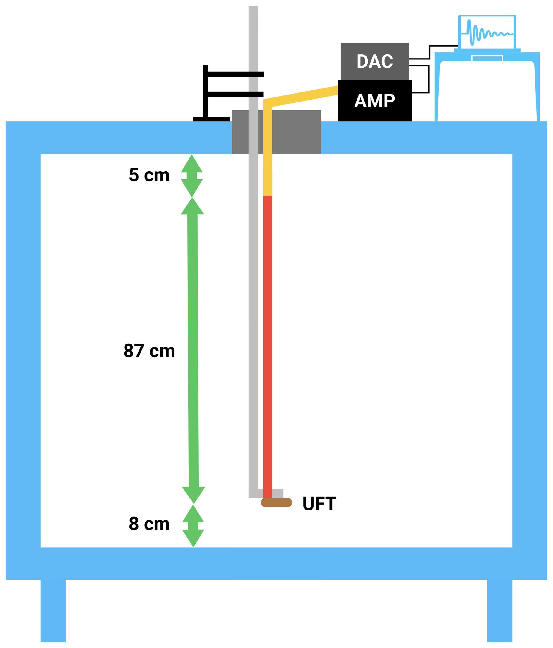
Figure 3 Schematic of the setup used during the measurements (diagram not to scale). At the top there was an operations center housing with most of the devices and cabling, including a BNC cable (yellow), a UFT amplifier (AMP), a digital-to-analog converter (DAC), and a PC with DAC software. Inside the Π Chamber, a vertical rod with a curved end (grey), a UFT sensor (brown), and a DANTEC^® probe support (red) attached to that end were deployed. The profiling limits were about 8 cm above the bottom and around 5 cm below the top layer. Note that, for clarity, the schematic does not include the cylindrical thermal panel, which was installed during the measurements.

For vertical profiling, the UFT was attached to a rod 6 mm in diameter and 1.5 m long with a 90° bend at the end. The rod was marked in 3 cm increments to facilitate easy UFT positioning. A sturdy metal stand with two adjustable clamps was used to secure the rod in a stable vertical position while allowing the user to manually move the UFT to the desired location (see Fig. 3). To minimize potential movements of the UFT cabling and sensor head, both were affixed to the rod using a simple adhesive, maintaining the wire in an upward orientation parallel to the floor.

We studied the small-scale temperature structure within the convection environment across three temperature differences between the chamber's floor and ceiling: 10, 15, and 20 K, as detailed in Table 1. The measurement setup included the cylindrical thermal panel (1 m height, 2 m diameter), which is not shown in Fig. 3. For a more detailed schematic, please refer to Chang et al. (2016). The Rayleigh number was on the order of ∼10⁹ for the set boundary conditions and the chamber height of 1 m. We performed our calculations based on the formula suggested by Niedermeier et al. (2018), assuming dry convection with an estimated Prandtl number of 0.72.

Table 1 List of experiments together with the corresponding Π Chamber and UFT settings as well as the Rayleigh numbers. Symbol explanation: T_F, T_C, and T_W represent the floor, ceiling, and wall temperatures, respectively. t stands for the measurement time at a given height h above the floor. The names of the experiments are formed as follows: type of measurement (“V” for vertical), ΔT, types of boundaries (“S” for smooth or “R” for rough), and time spent in a single position (“L” for 19 min or no marking for 3 min).

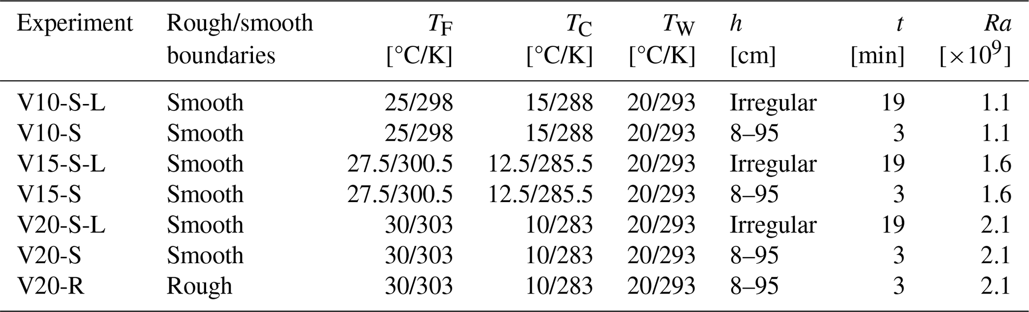
The irregular positions are 8, 14, 26, 35, 50, 65, 74, 86, and 95 [cm].

Our primary focus was on examining scalar fluctuations throughout the entire vertical dimension, with a particular emphasis on regions near the floor and the ceiling. To achieve this, the UFT deployments featured irregular measurement positions (see Table 1), increasing the spatial resolution of measurements slightly near both plates. Another consideration was the variable measurement time t, ranging from 3 to 19 min. Such a choice was dictated by the chamber's operational schedule, which constrained both the number of sampled points and the range of explored conditions. To quantify whether the measurements are converged, we employed the framework provided by Lenschow et al. (1994). According to the results presented by the authors, when the ratio of the measurement time t to the large-eddy correlation time t_c is $t/t_{\mathrm{c}}\approx \mathrm{10}$, the data are within approximately 10 % of the true value. Considering the turbulent properties, we link t_c to the large-eddy correlation time for the turbulence flow, which is estimated to be on the order of several seconds, i.e., 10 s in calculations, assuming a mean flow velocity of tens of centimeters per second. In this case, the averaging time of 3 min corresponds to approximately 18t_c, whereas for the 19 min time series it gives 114t_c, indicating satisfactory convergence for atmospheric applications.

A less emphasized aspect was the surface topography. One configuration involved the presence of rough boundaries, consisting of aluminum bars (4 cm wide and 1.4 cm high) positioned on the floor and ceiling, forming longitudinal stripes separated by 17 cm intervals. The bars themselves were at a slightly different temperature compared to the rest of both panels (approximately 0.4 K). Subsequent UFT deployments were conducted after removing the bars, aiming to compare temperature fluctuation properties between the two cases. Unfortunately, a portion of the dataset is invalid due to high battery drainage, resulting in coverage of only one rough boundary case in this study.

As the surfaces inside the chamber reached steady temperatures (see Table 1), the UFT sensor was initially positioned 8 cm above the floor near the axis of the cell. Due to the rod's length inside the chamber corresponding to its height, we had to wait for some time to allow the vibrations of the head sensor to dampen. This was really important after each position (h) change but played a crucial role in profiling the lower half of the measurement volume especially. The chamber's flange was covered with a thick foam layer, effectively reducing most mixing events near the opening. Although not an ideal solution, it seemed the most reasonable choice considering the ease of checking the UFT position and the insulating and damping properties of the foam (when coating the rod).

After completing the measurements, the dataset underwent several basic preparations. These included the removal of electronic artifacts, signal despiking, Butterworth filtering (10th order, 2 kHz cutoff frequency), 2 kHz averaging, and the translation of values from voltage to temperature units. Additionally, each time series was consequently normalized by subtracting the mean temperature value in the given position (see, e.g., Fig. 4).

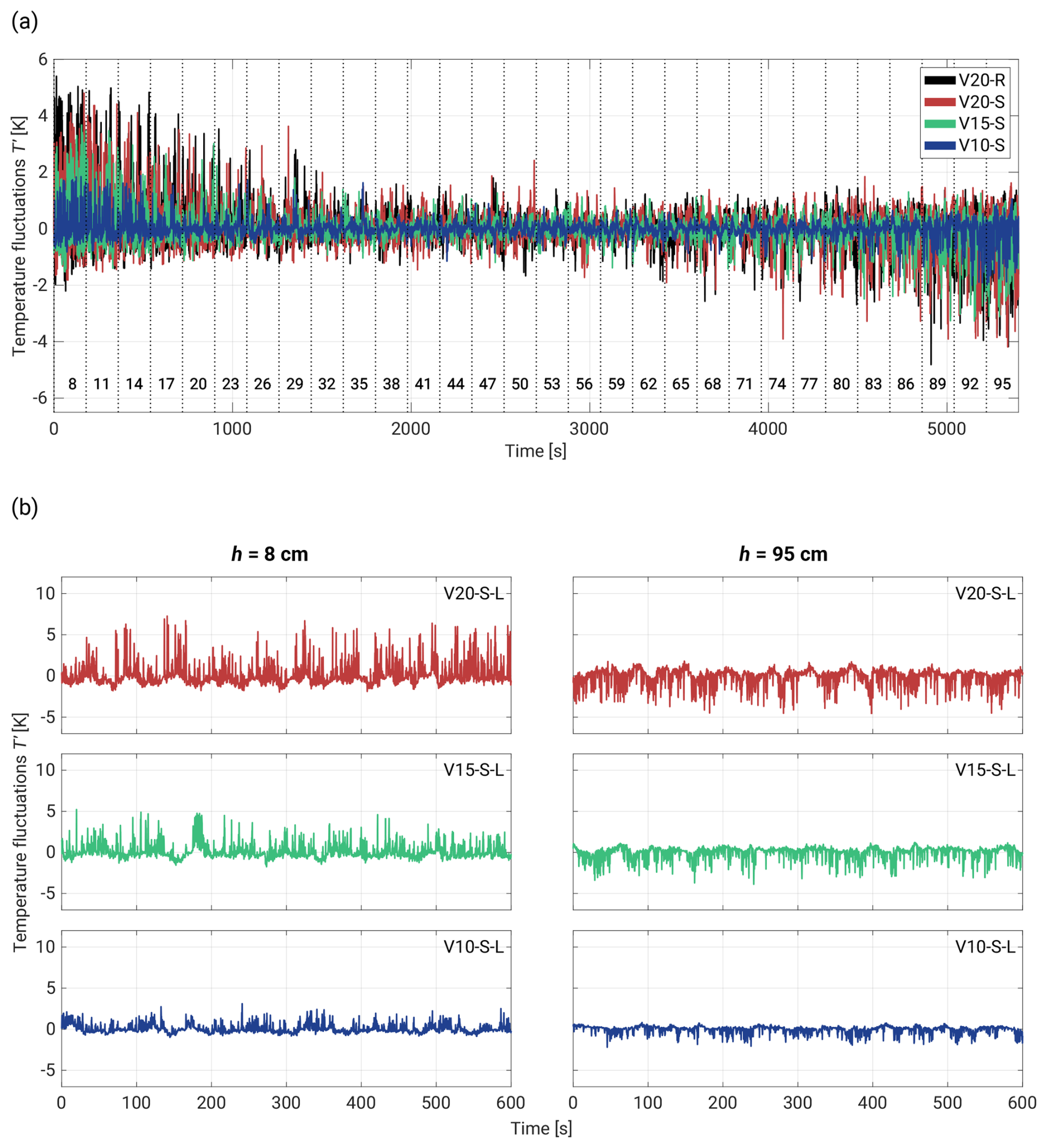
Figure 4 Temperature fluctuation T^′ time series corresponding to the different ΔT values that are described in Table 1. Panel (a) shows time series collected during full vertical scans, with consecutive changes in the sensor positions across the chamber. The horizontal row of numbers denotes the heights in centimeters above the lower plate. The chart includes 3 min series. Panel (b) shows 10 min measurements near the floor (h=8 cm) and just below the ceiling (h=95, 5 cm below the top plate).

2.2 DNS methodology

Cloud Model 1 (CM1) (Bryan and Fritsch, 2002) in DNS configuration is used for these simulations. The model and setup are described in detail in Chandrakar et al. (2022, 2023). The computational domain size for DNS is $\mathrm{960}\times \mathrm{960}\times \mathrm{500}$ grid cells with a homogeneous 2.083 mm grid spacing in the horizontal and a stretched grid in the vertical (finer near the top and bottom boundaries). Note that the computational domain represents a rectangular parallelepiped system rather than the cylindrical setup used during the experiments. CM1 solves the conservation equation set with the Boussinesq approximation and a prognostic pressure equation using a three-step Runge–Kutta time integration method with a fifth-order advection scheme. The Klemp–Wilhelmson time-split steps are used for the acoustic terms in the compressible solver. The time integration of the governing equations uses an adaptive time step with a maximum Courant–Friedrichs–Lewy (CFL) number of 0.8. A no-slip boundary condition for all of the walls is applied, and the temperature boundary conditions (constant temperatures) are the same as those of the experimental setup. The simulations use molecular viscosity and thermal diffusivity values at the mean temperature (Prandtl number =0.72). DNS is performed for the three experimental cases V20-S, V15-S, and V10-S listed in Table 1. Outputs from a steady-state period after the initial spinup are used for the analysis. Consistent with the experiments, the Eulerian temperature time series are outputted at 0.0012–0.0015 s intervals from a region near the center of the domain (95–105 cm from the side walls) at multiple heights from the bottom surface.

3 Results

3.1 Determination of basic characteristics of temperature profiles

Figure 4a provides a sample of temperature fluctuations T^′ ($T^{\prime }=T_h-{\stackrel{\mathrm{‾}}{T}}_h$, where T_h represents the temperature series at a given height h and the overline denotes the mean) from the vertical scan of the measurement volume near the axis of the chamber. The skewed fluctuations observed nearest to the plates serve as expected temperature evidence of thermal plumes characteristic of RBC. We can observe a smooth transition involving gradual suppression of fluctuations or rather a gradual decrease in occurring thermal plumes as the sensor moved towards the mid-height plane. The reverse symmetry is present in the upper half of the cell. The nature of these fluctuations aligns with the numerical results of heat fluxes in the bulk region obtained by Lakkaraju et al. (2012), temperature time series reported in He and Xia (2019) and Wang et al. (2022), and experimental data provided by Anderson et al. (2021). However, it is noteworthy that all these works focused primarily on specific regions of the cells, lacking more detailed insight into the temperature characteristics, especially considering the limited temporal resolution of the used instrumentation.

The most substantial temperature fluctuations are observed near the floor region. In cases with a flat surface (experiment summary in Table 1), peaks oscillate around 4 K, while rough boundaries can exhibit fluctuations exceeding 5 K. As the sensor approaches the mid-height plane, the differences between ΔT=20 K cases become negligible. Similarly, no distinctions are apparent near the upper plate, with a maximal amplitude at the level of −4 K for both V20-S and V20-R.

In Fig. 4b, two vertical layouts are presented, each illustrating 10 min series near both plate positions and segregating T^′ based on the given ΔT. The evident reverse symmetry is notable; however, it is important to highlight that there are varying amplitudes of fluctuations in each corresponding pair of graphs (same ΔT but different h). This variation may result from weaker thermal plumes departing from the top plate as well as from the imperfectly insulated chamber flange (mentioned in Sect. 2.1), which could lead to minor mixing in the vicinity of the sensor deployment spot. For a more in-depth examination of the temperature fluctuations near both plates, see Appendix A.

The temperature fluctuations also manifest oscillations that are particularly noticeable in the case of ΔT=20 K near the plates. However, these oscillations gradually decrease as the temperature difference decreases and the sensor moves towards the center of the cell. Analyzing V20-S-L at both heights, the periodicity appears irregular but is on the same order of magnitude as observed by Anderson et al. (2021), and therefore it corresponds to the LSC. Previous studies have highlighted that the LSC can exhibit various modes around its mean position, leading to phenomena such as out-of-phase oscillations at the top and bottom of the chamber (torsional mode; see Funfschilling et al., 2008) and side-to-side oscillations (sloshing mode; see Xi et al., 2009, and Brown and Ahlers, 2009). Cells with very high symmetry might also be characterized by spontaneous cessation and reorientation of the LSC to a different angular position (Brown and Ahlers, 2009). All these effects are beyond the scope of this investigation, but the raw measurements provide clear evidence of temperature oscillations near both plates.

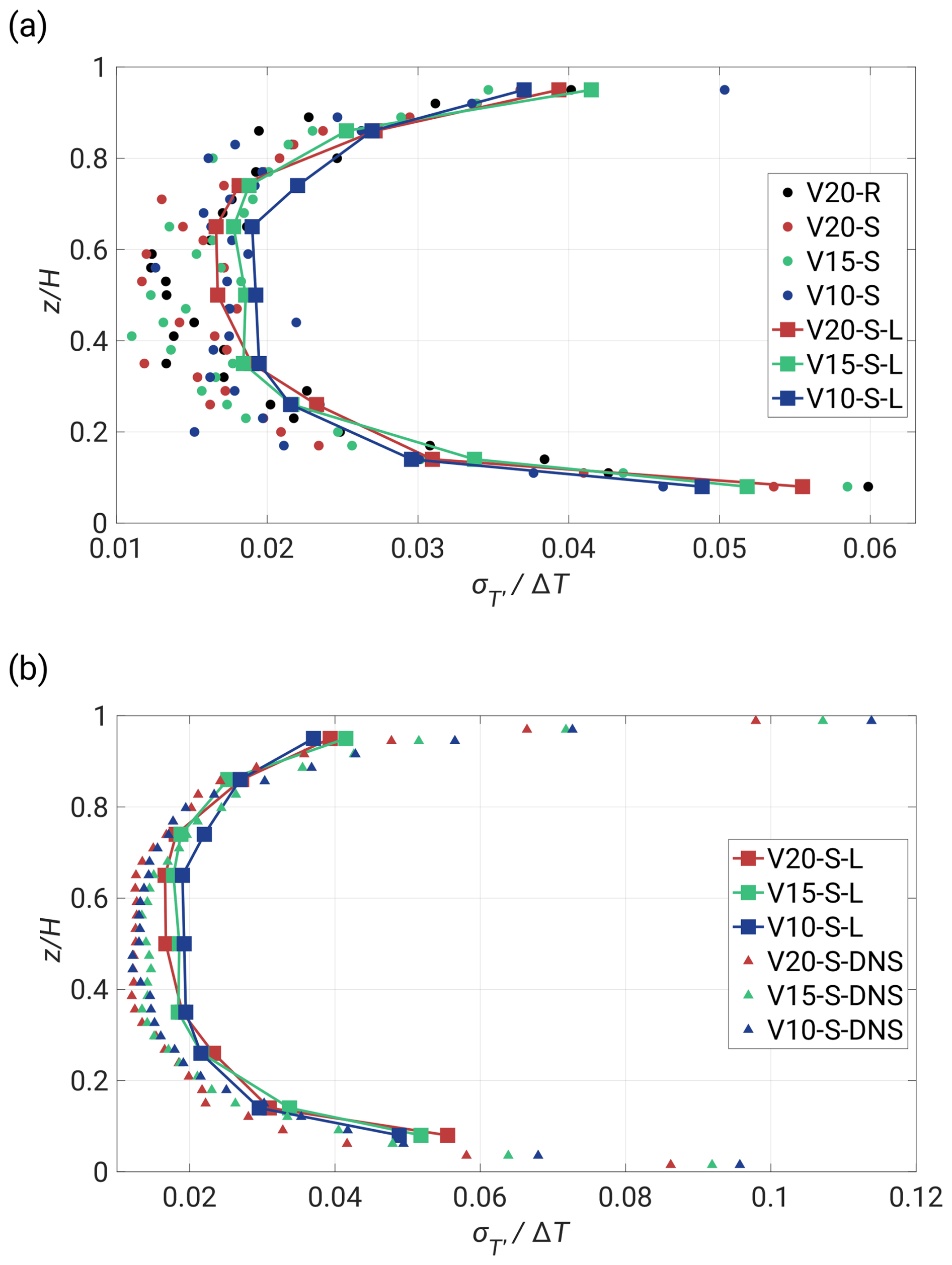
In Fig. 5, the standard deviation ${\mathit{\sigma }}_{T^{\prime }}$ is presented in relation to the sensor position within the chamber and illustrates the dependence of the fluctuation level, corresponding to Fig. 4a. The highest ${\mathit{\sigma }}_{T^{\prime }}$ values are observed near both plates, with the maximum at the bottom. This asymmetry diminishes as ΔT decreases, starting with an approximate 0.4 K disparity in V20-R and concluding with a shift of about 0.1 K in V10-S-L. It is noteworthy that extended measurements yield slightly different values, reflecting a more robust convergence as opposed to the 3 min cases. The bulk region exhibits relatively constant values with comparatively small deviations. Additionally, this region experiences the smallest differences between corresponding ΔT values. A decreasing ΔT shifts ${\mathit{\sigma }}_{T^{\prime }}$ values left and damps T^′ in the whole volume. In Fig. B1a we provide a non-dimensional form of the standard deviation.

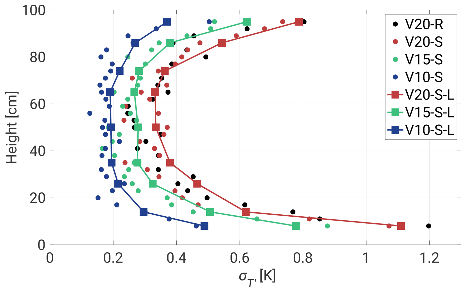
Figure 5 Standard deviation ${\mathit{\sigma }}_{T^{\prime }}$ with respect to the vertical position of the sensor. Short time series (3 min) are denoted by the circles, and the squares represent longer measurements (19 min). A decreasing ΔT shifts ${\mathit{\sigma }}_{T^{\prime }}$ values left, reducing the temperature fluctuations in all of the positions.

The surface topography contributes to slightly higher ${\mathit{\sigma }}_{T^{\prime }}$ values, primarily nearest the plates. This effect may be attributed to the elevated surface level, potentially leading to varied stages of thermal plume development in the same measurement position. However, these thermal structures are becoming mixed with the surroundings, producing approximately equivalent results just a few centimeters higher. As mentioned previously, He and Xia (2019) emphasized that each region of the RBC can exhibit its local dynamics, a consequence of overlapping mechanisms that act as drivers of each other. In this specific case, the LSC induces mixing of all thermal structures originating from the surface. It can also turbulently propel thermal plumes due to irregular topography. The resulting mixing and stronger turbulence in this region might be responsible for the thermal peaks observed in Fig. 4a.

In Fig. 6, the skewness of T^′, denoted as ${\mathit{\gamma }}_{T^{\prime }}$, is analyzed with respect to the vertical positions within the chamber. We use an adjusted Fisher–Pearson standardized third moment, expressed as ${\mathit{\gamma }}_{T^{\prime }}=\frac{N^{\mathrm{2}}}{(N-\mathrm{1})(N-\mathrm{2})}\frac{{\stackrel{\mathrm{‾}}{T^{\prime }}}^{\mathrm{3}}}{{{\mathit{\sigma }}_T^{\prime }}^{\mathrm{3}}}$, where N represents the number of samples. The findings confirm previous observations, showing positive skewness (associated with warm plumes) near the floor and negative skewness (indicative of cold plumes) just below the ceiling. The third moment is notably influenced by rare events, leading to significant fluctuations in the 3 min dataset, but these are mostly averaged out in longer segments, resulting in more consistent curves.

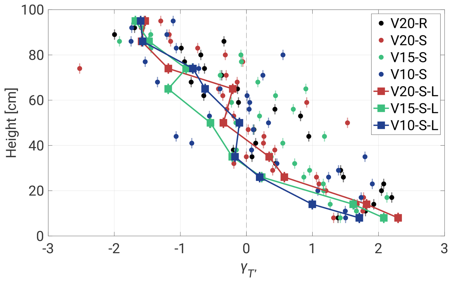
Figure 6 Skewness ${\mathit{\gamma }}_{T^{\prime }}$ with respect to the vertical position of the sensor. Short time series (3 min) are denoted by the circles, and the squares represent longer measurements (19 min). Uncertainties were calculated using the formula ${\mathit{\delta }}_{{\mathit{\gamma }}_{T^{\prime }}}=\sqrt{\frac{\mathrm{6}N(N-\mathrm{1})}{(N-\mathrm{2})(N+\mathrm{1})(N+\mathrm{3})}}$, where N denotes the number of samples.

The regions near both plates demonstrate data convergence of ${\mathit{\gamma }}_{T^{\prime }}$ values with minimal deviations. An interesting observation is noted at a distance of 8 cm above the floor, where the 3 min records initially exhibit a skewness of about 1.4. This area likely experiences a higher frequency of intense thermal plumes, resulting in a broader range of temperature fluctuations (see Fig. 5). It has been shown in previous studies that thermal plume detachment introduces large fluctuations in temperature and velocity boundary layer thickness (Wagner et al., 2012; Shi et al., 2012; De et al., 2018; Shevkar et al., 2022). Similar effects might be responsible for what we observe. As the plume structures develop, ${\mathit{\gamma }}_{T^{\prime }}$ increases to approximately 2. Then, at the 20 cm level, there is a subtle indication of a possible change in the thermal dynamics of the system. This change may be associated with specific transitions in convective flow patterns and more intense interaction of thermal plumes with the LSC in the ring layer around the walls and plates (see Fig. 2a). Moving further away from the heated floor, the LSC is likely dominating the existing structures, increasing the dissipation of thermal energy and leading to a decrease in skewness. This results in thermal structures becoming more dispersed, leading to a narrower and less extreme distribution of temperature fluctuations.

However, not all thermal plumes could be averaged out fully, especially as the flow around the cell decreases towards more central regions. This might allow some remaining plume structures to reach the central region between 40 and 70 cm and mix, which could result in positive skewness (bottom plumes carry higher energy). Similar behavior might also be observed in longer records, manifesting as fluctuations in ${\mathit{\gamma }}_{T^{\prime }}$ within the 50–70 cm segment. Importantly, the positions of these shifts do not appear to be directly dependent on ΔT.

A comprehensive understanding of the thermal dynamics requires additional information on the small-scale temperature field around the axis, its velocity field, and a detailed description of the LSC time evolution. From the perspective of microphysical processes in future moist experiments, the Lagrangian histories of droplets or aerosols carried by thermal plumes – or alternatively located in the volumes between them – can theoretically lead to different droplet sizes (Chandrakar et al., 2018b, 2023). The local variability of ${\mathit{\sigma }}_{T^{\prime }}$ and ${\mathit{\gamma }}_{T^{\prime }}$ indicates that, over short timescales, droplets present in a given volume of the chamber may develop differing growth habits.

Upon comparing the topographic effect, we did not observe any major differences and concluded that 3 min records might be insufficient for investigating the impact caused by the presence of roughness. However, recent numerical work by Zhang et al. (2018) (for ${\mathrm{10}}^{\mathrm{7}}⩽\mathit{\text{Ra}}⩽{\mathrm{10}}^{\mathrm{11}}$ and fixed Pr=0.7) indicates that there is a critical roughness height h_c below which the presence of roughness reduces heat transfer in RBC. The authors link this phenomenon to fluid being trapped and accumulated inside the cavity regions between the rough boundaries. Our approximate calculations for the Π Chamber setup indicate an h_c value of approximately 7 mm compared to the 1.4 cm height of the tiles.

3.2 Power spectral densities

The power spectral density (PSD) of T^′ was computed using the Welch algorithm. Initial analyses were primarily directed towards estimating the LSC periods τ for the given ΔT and with respect to the measurement position (see Fig. 7a). This involved utilizing 19 min datasets with window lengths approximately equal to the sizes of the collected segments. Employing a 50 % overlap between segments and incorporating a high number of discrete Fourier transforms (8 times the window length), we derived estimates of the LSC periods along with their associated standard deviations. For ΔT=10 K, a modest convergence of data points is observed, which is particularly notable within the 60–80 cm region. This resulted in a relatively elevated standard deviation (grey areas denote ±1σ_τ), yielding a period of approximately τ₁₀≈79 s. Subsequent ΔT demonstrated a more uniform distribution across all of the levels, accompanied by gradual reductions in the LSC period to approximately τ₁₅≈65 s and τ₂₀≈57 s.

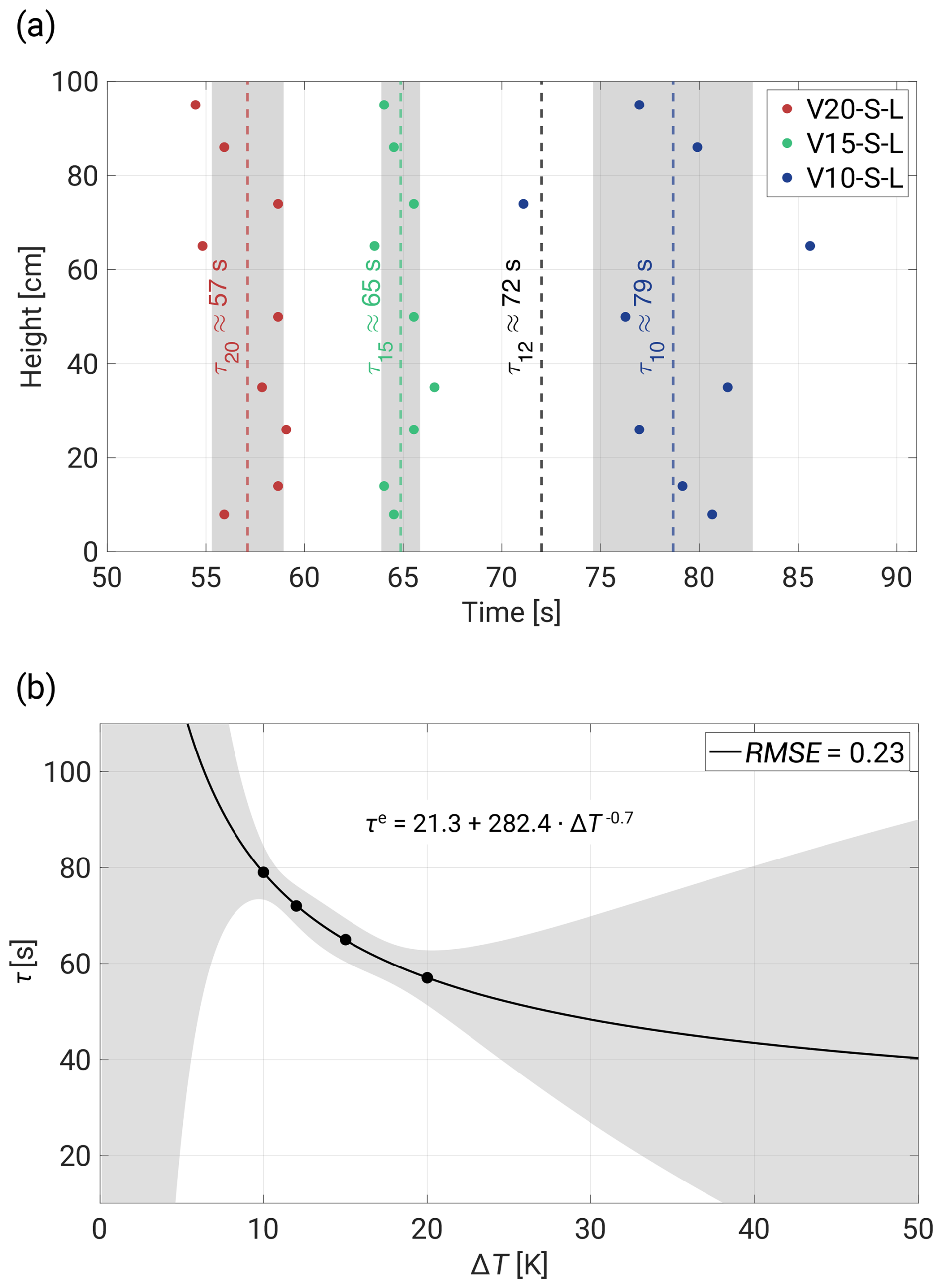
Figure 7 Measured LSC periods with respect to ΔT and the vertical position of the sensor. (a) The grey regions describe ±1σ_τ, and the black dashed line denotes the result obtained by Anderson et al. (2021) for ΔT=12 K. (b) The relationship between τ and ΔT modeled by the power law (τ^e) function. The plot includes 95 % simultaneous functional bounds, a fitted equation, and the root mean squared error (RMSE).

The relationship between τ and ΔT, modeled by the power law function τ^e, is illustrated in Fig. 7b. The fit exhibits narrow 95 % prediction bounds in the fitted region but significantly large bounds outside it. The model was constructed using a sparse dataset consisting of only four data points, including the result obtained by Anderson et al. (2021) at ΔT=12 K. Consequently, this limited dataset may not fully capture the true relationship, particularly at lower (ΔT<10 K) and higher (ΔT>20 K) temperature differences. The potential discrepancies could be due to a stronger diffusion dominance over convection at lower ΔT or more pronounced overlapping thermal plumes at higher temperatures.

In subsequent PSD analyses, we continued using only 19 min records, as shorter measurements exhibit too much variability in spectra due to their duration being comparable with the LSC periods. This time-modified window length, approximately one-ninth of the total segment with windows overlapping by half their length, resulted in 17 individual PSDs that were averaged. This approach enhances chart readability while maintaining fidelity to the spectral slopes. To collapse the curves representing measurements from different positions, we followed the scaling method proposed by Zhou and Xia (2001). Figure 8a plots the scaled f²P(f) spectrum for the V20-S-L case, enabling determination of the peak frequency f_p, around which the PSDs become universal functions. In this case, f_p oscillates around f=4 Hz, exhibiting high convergence across all of the curves.

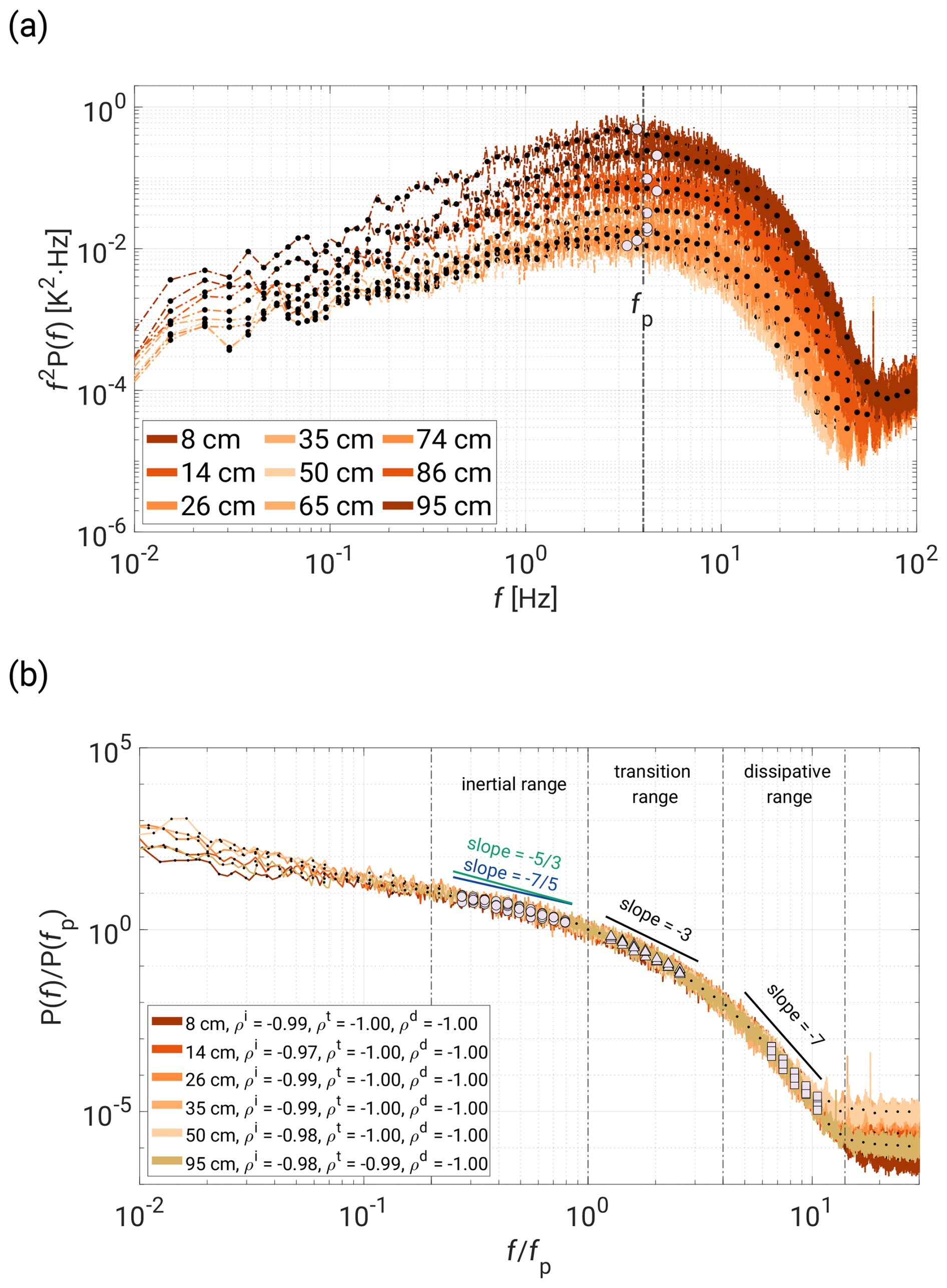
Figure 8 Scaled V20-S-L PSD with respect to the UFT positions (color gradients) in the chamber. (a) Scaled spectrum of f²P(f) across the chamber volume and with a marked mean f_p value of f_p≈4 Hz. (b) PSD $P\left(f\right)/P\left(f_{\mathrm{p}}\right)$ versus $f/\left(f_{\mathrm{p}}\right)$ with three defined regimes: inertial range (circles, $\mathrm{0.2}⩽f/f_{\mathrm{p}}⩽\mathrm{1}$), transition range (triangles, $\mathrm{1}⩽f/f_{\mathrm{p}}⩽\mathrm{4}$), and dissipative range (squares, $\mathrm{4}⩽f/f_{\mathrm{p}}⩽\mathrm{20}$). Each regime is denoted by different markers, with an approximate slope value added above the curves. The Pearson correlation coefficients p have upper indices to indicate the regimes. Please note that the results presented in panel (b) cover positions from the lower half of the chamber as well as the top position.

In Fig. 8b, we provide a sample of the scaled PSD $P\left(f\right)/P\left(f_{\mathrm{p}}\right)$ versus $f/f_{\mathrm{p}}$ in the lower half of the chamber and define three spectrum regimes. Based on the scaling method proposed by Kumar and Verma (2018) and Zhou and Xia (2001), we also conducted a similar analysis in the wavenumber domain. For more details, please refer to Appendix C. To estimate the slopes, we employed a methodology outlined in Siebert et al. (2006) and Nowak et al. (2021), averaging raw spectra over equidistant logarithmic frequency bins (20 bins per decade in our case) and then fitting power law functions. To obtain the best possible fit, we selected spectral regions based on the highest log–log linearity criteria, using the Pearson correlation coefficient p for the resampled points.

Extended discussions on passive scalar spectrum scaling can be found in works such as Gotoh and Yeung (2012) and Sreenivasan (2019). We adapted the graph from the former study for Fig. 9, which illustrates possible spectral slopes as a function of the Pr number. For our experimental conditions, the results are expected to align with the scaling for Pr≈1. In the following paragraphs, we aim to contextualize our findings within the broader scope of the literature and to address potential explanations for observations that have not yet been described.

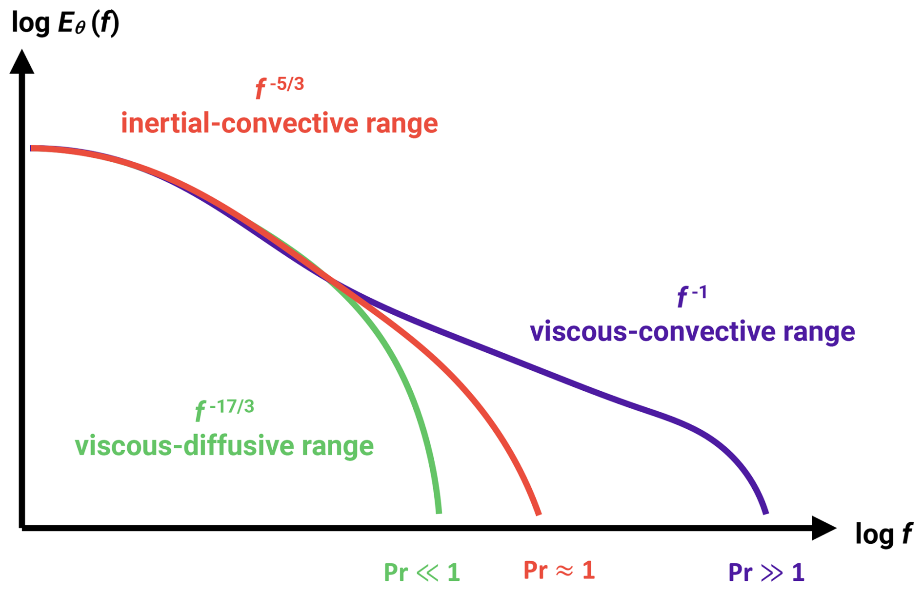
Figure 9 Schematic of the passive scalar spectrum depending on the Pr regime. The figure is based on the graph from Gotoh and Yeung (2012), with minor modifications.

In Fig. 10a, the regime $\mathrm{0.2}⩽f/f_{\mathrm{p}}⩽\mathrm{1}$, marked by circles, in the literature is referred to as the inertial-convective regime, which is associated with OC scaling where the temperature field (acting as a passive scalar) does not influence the flow dynamics (Castaing, 1990; Cioni et al., 1995; He et al., 2014). However, in thermally driven convection, the flow is actively driven by temperature-induced buoyancy differences. This range is therefore redefined as the inertial-buoyancy range, where the temperature spectrum follows BO scaling (Chillá et al., 1993; Ashkenazi and Steinberg, 1999; Zhou and Xia, 2001). Our analysis provides no definitive answer, as the slopes oscillate between OC and BO scaling, with a slight bias towards $-\mathrm{7}/\mathrm{5}$. However, as noted previously, the two slopes are too close to be distinguished easily (see Fig. 8b). Thus, we classify this range simply as the inertial range without committing to a specific scaling profile. Interestingly, Niemela et al. (2000) (${\mathrm{10}}^{\mathrm{6}}⩽\mathit{\text{Ra}}⩽{\mathrm{10}}^{\mathrm{7}}$) and Pawar and Arakeri (2016) (axially homogeneous buoyancy-driven turbulent flow, ${\mathrm{10}}^{\mathrm{4}}⩽\mathit{\text{Ra}}⩽{\mathrm{10}}^{\mathrm{9}}$) observed both scaling behaviors in their experiments. The latter study raised the question of whether these results indicate dual scaling or a gradual steepening of the spectrum.

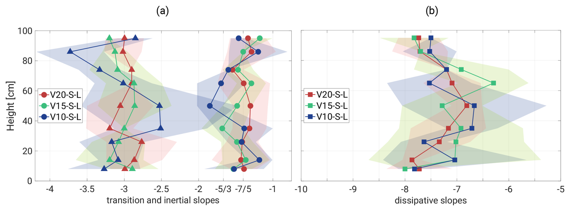
Figure 10 Vertical variation in the fitted PSD slopes. Panel (a) corresponds to the transition (triangles) and inertial (circles) ranges, respectively, whereas panel (b) describes the dissipative regime. The slopes are accompanied by 95 % confidence bounds, except in a few cases where the slopes were manually fixed due to fitting difficulties.

No direct references in the literature address the subsequent regime scalings ($\sim -\mathrm{3}$ and $\sim -\mathrm{7}$) or the roll-off region of the scalar spectrum (see Fig. 9). Recent investigations of the dissipation range in the energy spectrum have only begun exploring this regime, suggesting a superposition of two exponential forms (Khurshid et al., 2018; Buaria and Sreenivasan, 2020). Therefore, our further discussion will explore potential connections between our and other results in convective flow research.

The −3 scaling might simply represent a crossover into the following dissipative range, but the mid-range scales in the system could also be subjected to more subtle phenomena. RBC dynamics span a wide range of scales, including thermal plumes, vortices, and the LSC, with complex interactions between these structures (Fernando and Smith, 2001; Xi et al., 2004; Zhou et al., 2016; Guo et al., 2017; Chen et al., 2018; Pandey et al., 2018; De et al., 2018; Dabbagh et al., 2020; Wang et al., 2022; Yano, 2023; Yano and Morrison, 2024). These overlapping processes likely influence the observed spectra. Recent LES studies on thermal plumes revealed additional insights into scalar spectral scaling (Chen and Bhaganagar, 2021, 2023, 2024). Using a heated surface experiment, the authors reported the density and temperature spectrum scaling to be −2.7, which was strongly correlated with the velocity spectrum. Furthermore, vertical heat and mass fluxes exhibited a −3 scaling, matching the vertical component of the turbulent kinetic energy (TKE) spectrum. This corresponds to the regime $\mathrm{1}⩽f/f_{\mathrm{p}}⩽\mathrm{4}$ marked by triangles in Fig. 10a, which is characterized by slopes oscillating around −3, with slightly greater variability observed for the V10-S-L case.

Moreover, in the papers of Chen and Bhaganagar, both spectra of the 2D TKE and horizontal structures of the 3D TKE and helicity consistently exhibited slopes of $-\mathrm{5}/\mathrm{3}$ and −3, respectively. Their flux analysis revealed an inverse TKE and helicity cascades towards large structures and forward cascades of these invariants for small scales. Further studies on velocity-based longitudinal structure functions (second, third, and fourth moments) showed that the scaling exponents fell between theoretical predictions for 2D and 3D systems. For example, strong vertical confinement or anisotropic Fourier mode distributions can mimic 2D dynamics in certain ranges (Musacchio and Boffetta, 2019; de Wit et al., 2022; Alexakis, 2023). Consequently, energy cascades and their directions are highly scale-dependent, influenced by invariants such as enstrophy and helicity, potentially resulting in the coexistence of multiple cascades and the superposition of power law spectra. Detailed discussions on cascades and transitions in turbulence are provided by Alexakis and Biferale (2018). However, in the Π Chamber, we do not recognize strong anisotropy, and only regions near the top and bottom plates could potentially exhibit such quasi-2D effects, whereas similar spectral slopes are observed in the entire volume of the chamber. On the other hand, in 3D turbulence, large-scale stirring can introduce helicity, modifying cascade directions and contributing sub-leading corrections, depending on the helicity's sign (Eidelman et al., 2014; Yan et al., 2020; Plunian et al., 2020). The exact role of helicity in energy transfer mechanisms remains unclear and is an active area of research (Yao and Hussain, 2022).

Given this complexity, it is reasonable to question whether theoretical assumptions such as isotropy, homogeneity, stationarity, and self-similarity are sufficient to capture the full physical reality. Anisotropy and nonstationary coherent structures likely play significant roles, potentially causing deviations from the predicted spectral scaling. In the RBC, temperature forcing drives both large- and small-scale structures, complicating the universality of passive and active scalar theories. Alexakis and Biferale (2018) emphasize that strong assumptions about cascades and their directions are not feasible for active scalars, particularly when velocity and scalar fields are strongly coupled. This leaves open questions about preferential sampling effects of forcing along Lagrangian trajectories of the active scalar field. In the given full-spectrum analysis, the nature of the spectral break observed near $f/f_{\mathrm{p}}\approx \mathrm{1}$ may be linked to a transition between LSC-dominated scales characterized by large coherent structures and smaller-scale thermal plumes and vortices. These overlapping power laws could ultimately shape the observed spectra. Consequently, we interpret the −3 regime as a transition range between buoyancy-scale processes and molecular dissipative scales. Additional analysis presented in Appendix D estimates the dominance of thermal plumes near the chamber center. Following He and Xia (2019), we demonstrate a logarithmic dependence of ${\mathit{\sigma }}_{T^{\prime }}$ on chamber height, reflecting a balance between buoyancy and inertial forces.

Finally, our high-frequency measurements indicate that the dissipative regime slopes are approximately −7 (see Fig. 10b). The slope distribution with respect to chamber height is symmetrical, reaching the largest values near the plates ($\sim -\mathrm{8}$) and the smallest values in the bulk region ($\sim -\mathrm{7}$). According to Sreenivasan (2019), no scalar spectrum description exists for the dissipative regime. While the energy spectrum in this range can be represented by an exponential form, our findings suggest that, for the scalar field, even a single power law is sufficient. Corresponding characteristics are visible in Niemela et al. (2000) and Zhou and Xia (2001), although these studies provide a limited discussion of the observed slopes.

Also worth noting is the variability of the noise level (starting around $f/f_{\mathrm{p}}\approx \mathrm{12}$) with respect to the chamber height, with its highest values linked to the bulk region and its lowest values (10 times magnitude difference) representing regions near the plates (see Fig. C1 in Appendix C). This phenomenon is due to the mean velocity field and its strong reduction in the central areas of the cell causing the noise to rise.

3.3 Comparison of DNS and experimental data

Another goal of the presented study was to compare the experimental results obtained with the UFT and the corresponding DNS data. The essential details of the DNS methodology and the properties of the series can be found in Sect. 2.2. Our approach was to repeat the analysis and retrieve basic characteristics of temperature profiles and information on PSDs at different vertical levels. Sample series can be seen in Figs. A1 and A2.

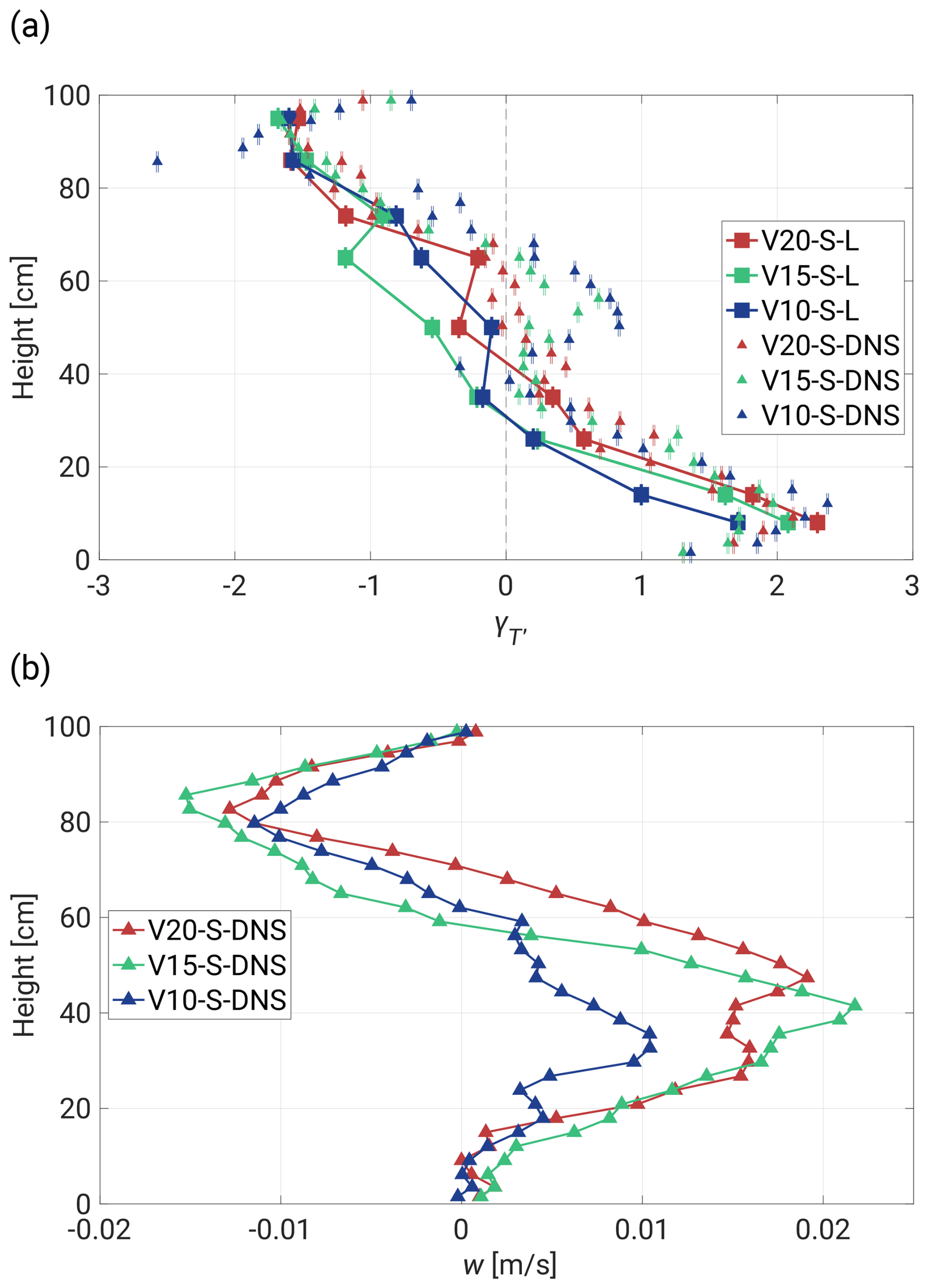
Figure 11 is analogous to Fig. 5 but presents the DNS data with exactly the same thermodynamic conditions as the experiment. Since the vertical grid size spans from about 1 mm near the plates to about 2.3 mm at the center, the available range significantly improves the comprehensiveness of the boundary layers. Regions near the top and bottom exhibit a maximum deviation of ${\mathit{\sigma }}_{T^{\prime }}\approx \mathrm{2}$ K with a bias in the vicinity of the upper plate. Also, the shape of the curves is more indented in the center and shifted slightly left, which might be analogous to the 3 min records in Fig. 5. The numerical data provide more stable monotonicity but represent equivalent periods of time as the experiment. Figure B1b shows a non-dimensional form of the same figure.

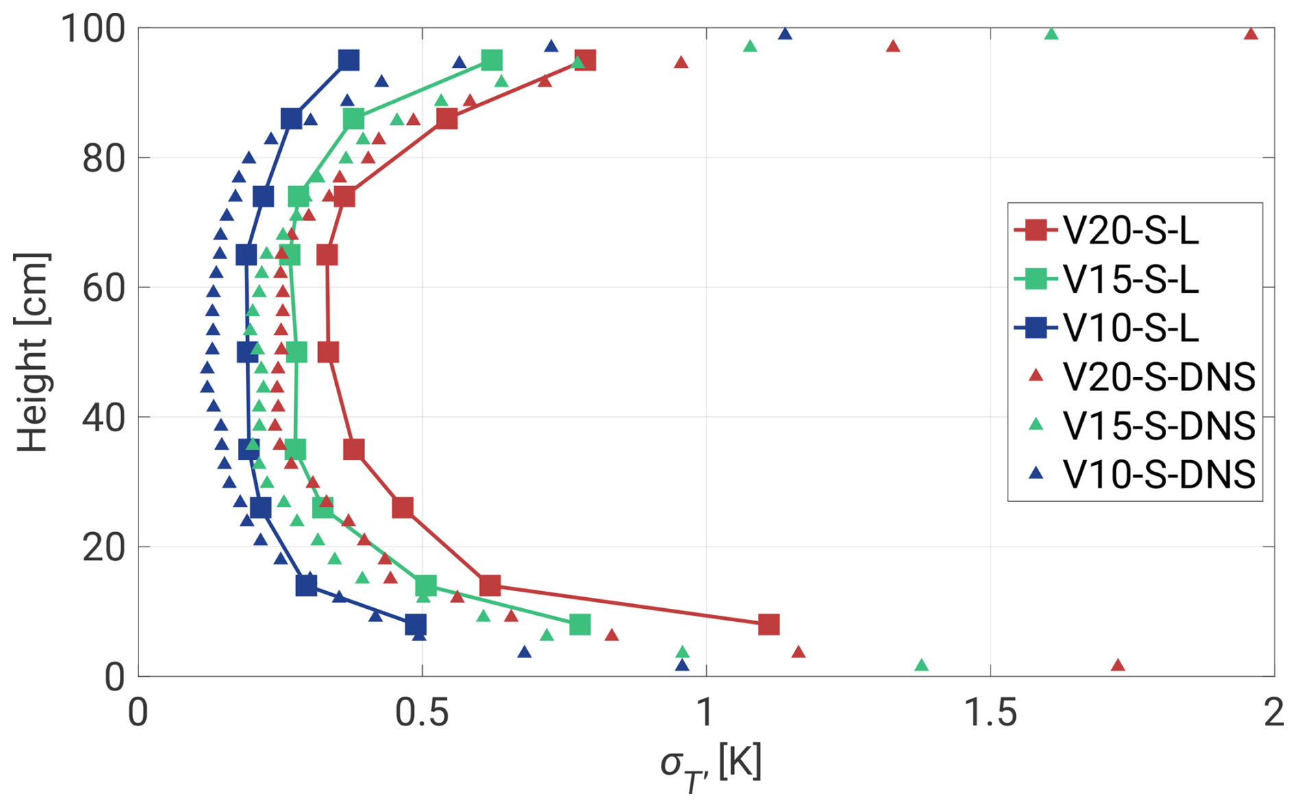
Figure 11 Standard deviation ${\mathit{\sigma }}_{T^{\prime }}$ with respect to the height of the chamber. The chart is analogous to Fig. 5 but only includes the 19 min segments (squares) and the DNS (triangles).

Similar conclusions can be drawn in terms of the skewness profiles in Fig. 12a. The DNS data exhibit much smaller fluctuations than the corresponding 3 min UFT segments but preserve the general tendency near the floor and in the central region. The characteristic jump in ${\mathit{\gamma }}_{T^{\prime }}$ is observed not around 20 cm, but halfway. On the other hand, a symmetrical jump is also observed near the ceiling, which was not revealed by the UFT measurements, likely due to a very shallow layer of the thermal plume regime (the UFT measurements ended about 5 cm below the ceiling). Also, the mixing region between 40 and 70 cm is re-established, resulting in higher deviations for lower ΔT. The skewness distribution contributes to the mean vertical flow profile in the cell (see Fig. 12b). The presence of both positive (∼40 cm) and negative (∼80 cm) velocity jumps drives dynamics in the bulk region, facilitating the mixing of cold and warm plumes. The horizontal components of the flow follow the LSC directions, giving a mean value of 15 cm s⁻¹ near the plates. A more comprehensive discussion of the dynamics of the thermal plumes can be found in Sect. 3.1. Note that the plots in Figs. 11 and 12 represent single-column data (not the horizontal average), meaning that perfect symmetry is not expected, in particular for the period of the LSC.

Figure 12 (a) Skewness, ${\mathit{\gamma }}_{T^{\prime }}$, as a function of height within the chamber supported by the 3 min DNS data. The chart is analogous to Fig. 6 but only includes the 19 min segments (squares) and the numerical time series (triangles). (b) Mean vertical flow profile provided by the DNS.

4 Summary

We conducted a small-scale study on the temperature structure of RBC in the Π Chamber using three temperature differences (10, 15, and 20 K) at an Ra of approximately 10⁹ and a Pr of 0.7. The objective was to improve our understanding of thermally driven convection by analyzing small-scale variations along the chamber's axis. Measurements were performed using a miniaturized UltraFast Thermometer operating at 2 kHz, enabling undisturbed vertical temperature profiling from 8 cm above the floor to 5 cm below the ceiling. Unlike classical RBC studies, this research is characterized by relatively short measurement durations of 19 and 3 min, which fall below the typical record lengths for such experiments. Nevertheless, the primary goal was to link this work to other experiments conducted in the Π Chamber. Its main objective was to investigate microphysical processes relevant to the real atmosphere, such as supersaturation fluctuations crucial to cloud formation and development. Small-scale temperature profiling under varying conditions, as typically observed in the chamber, provides valuable insights that could inform future experiments and address related scientific questions. The key findings of this study are summarized below.

• Basic characteristics. We observed significant changes in the standard deviation and skewness of the distribution of temperature fluctuations near the top and bottom surfaces. Additionally, we see variations in the spectrum scaling in these near-surface regions. The turbulence in the center of the chamber exhibited characteristics more akin to homogeneous isotropic turbulence. These observed variations were attributed to the dynamics of local thermal plumes and their interaction with the large-scale circulation (LSC). Both 19 and 3 min measurements were consistent, although the shorter records showed a higher variability in the standard deviation and skewness distribution. The statistical properties of the temperature field obtained in the Π Chamber may offer insights into thermal structure development in the atmospheric surface layer, thereby enhancing our understanding of surface–air temperature fluctuation characteristics with respect to thermal conditions (Kukharets and Nalbandyan, 2006). Furthermore, the analysis of large-scale coherent structures in RBC provides a framework for broader perspectives on thermal circulations and the distribution of temperature and moisture, both in cloud chambers (Anderson et al., 2021) and by analogy in the lower atmosphere (Zhou and Xia, 2013; Moller et al., 2021). The chamber is not designed for idealized RBC experiments. Its structure solutions (e.g., windows on the sides, atypical sidewall boundary conditions) aimed at cloud microphysics research are revealed in asymmetries of the profiles of temperature fluctuation statistics.

• Topographic effects. No major differences were observed that corresponded to topographic effects, likely due to insufficient time series. However, numerical work by Zhang et al. (2018) shed light on the necessary roughness height for robust heat transfer in RBC. Below the critical point, the authors observed trapped and accumulated heat inside the cavity regions between the rough boundaries.

• Dynamic regimes. PSD analysis revealed periodicity of LSC with respect to the temperature differences and characterized by the power law formula, consistent with previous findings (Anderson et al., 2021). We identified three distinct dynamic regimes: an inertial range (slopes of $\sim -\mathrm{7}/\mathrm{5}$), a transition range (slopes of $\sim -\mathrm{3}$), and a dissipative range (slopes of $\sim -\mathrm{7}$). The scale break between the inertial and transition ranges was attributed to a dynamic transition from the LSC-dominated regime to the thermal plume regime. Appendix D demonstrates that this transition is also observable in the spatial domain. Our findings are consistent with other studies not directly related to RBC. For example, a similar scale break between the inertial and transition ranges was observed in temperature fluctuation measurements near the surface of Jezero Crater on Mars (de la Torre Juárez et al., 2023), whereas slopes of $-\mathrm{17}/\mathrm{3}$ and −3 have been reported in power spectra of the solar surface intensity variance field, which are attributed to buoyancy-driven turbulent dynamics in a strongly thermally diffusive regime (Rieutord et al., 2010).

• Experiment versus DNS. Experimental findings showed convincing agreement with DNS conducted under similar thermodynamic conditions, marking a rare comparative analysis in this field. Velocity profiles supported the argument for the nature of thermal plumes, and a method to convert spectra from the frequency domain into the wavenumber domain was detailed (see Appendix C). Despite the presence of imperfect boundaries such as window flanges, sampling ports, and instrumentation, idealized DNS provided a reasonable representation of the actual Π Chamber flow, indicating that DNS adequately resolves surface layer fluxes. These results are valuable for improving and validating numerical research, such as subgrid large-eddy simulation models (Salesky et al., 2024) and heat transport models (Goluskin, 2015).

Appendix A: Quick looks at temperature fluctuations

The figures illustrate two realizations of temperature fluctuations at the sensor's position under similar conditions (from the experiment and DNS). The presence of filaments or coherent structures, with temperatures close to that of the nearby plate, is clearly visible. It is important to note that this is not a one-to-one comparison of the same flow but rather an illustration of the maximal scalar fluctuations observed in both the simulation and the experiment. Despite differences in the time resolution, both curves in each case exhibit similar magnitudes. The subsequent zoomed-in segments further emphasize the variability within these realizations.

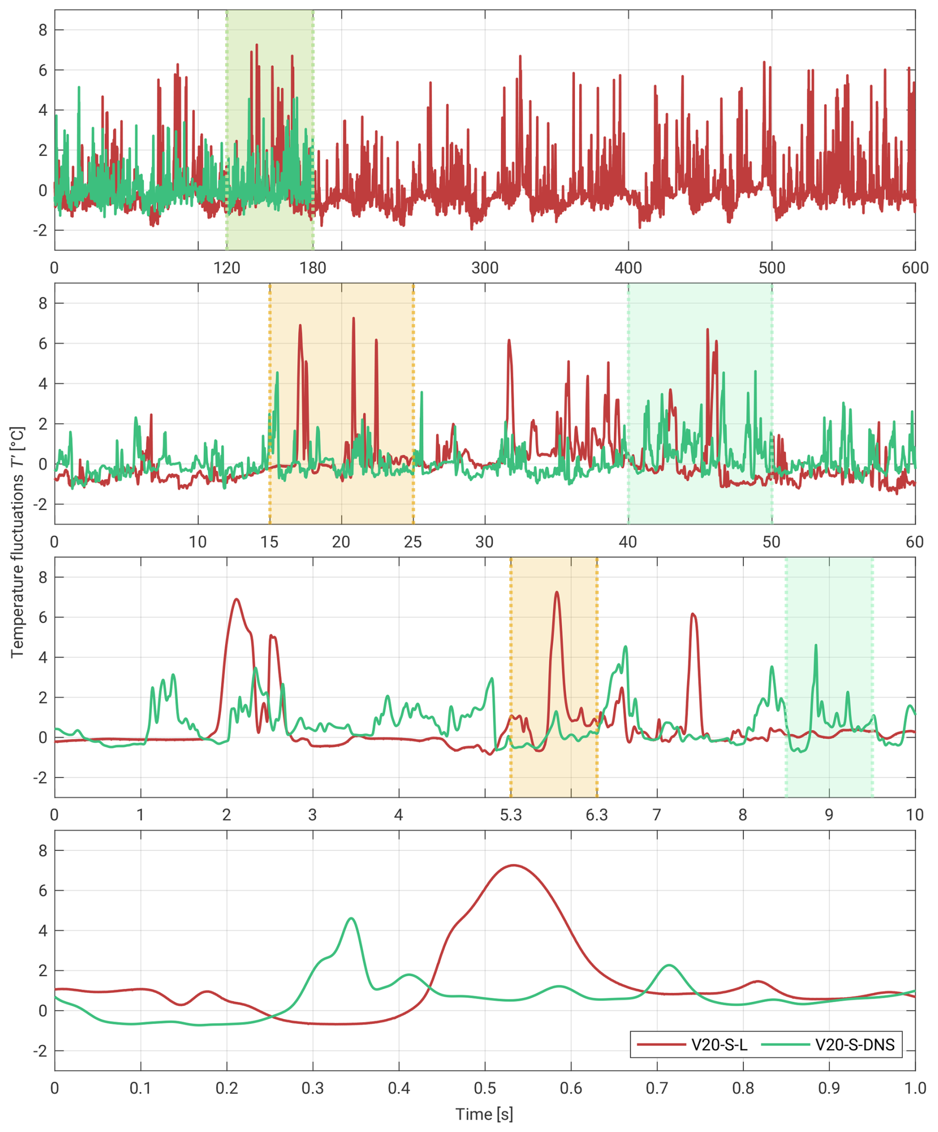
Figure A1 Experimental versus DNS T^′ series ∼8 cm above the floor shown in the following zoomed-in time segments: 600, 60, 10, and 1 s. The presented dataset is from the ΔT=20 K case. Please note that the time series from the experiment and the DNS do not correspond to each other.

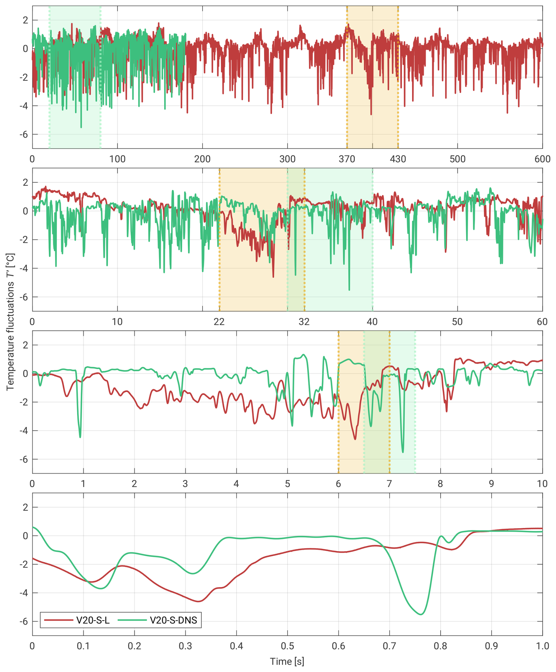
Figure A2 Experimental versus DNS T^′ series ∼5 cm below the ceiling shown in the following zoomed-in time segments: 600, 60, 10, and 1 s. The presented dataset covers the ΔT=20 K case. Please note that the time series from the experiment and the DNS do not correspond to each other.

Appendix B: Non-dimensional representations of standard deviations

Non-dimensional profiles of the standard deviation show stronger convergence in longer records compared to their dimensional representations.

Figure B1 Non-dimensional standard deviation scaled by the corresponding ΔT. In the figure, $z/H$ represents the vertical distance z measured from the bottom plate and normalized by the cell height H=1 m. (a) Analogous to Fig. 5. (b) Analogous to Fig. 11.

Appendix C: Power spectral density in the wavenumber coordinate

In the atmospheric community, PSD is typically presented in either the frequency domain or the wavenumber domain, depending on preferences or scientific goals. As demonstrated in Sect. 3.2, the collapsed spectral curves in the frequency domain exhibit three dynamic regimes that characterize thermal convection in the Π Chamber. However, by following the scaling method proposed by Kumar and Verma (2018) and the generalized approach of Zhou and Xia (2001), one can obtain an analogous PSD in the wavenumber domain.

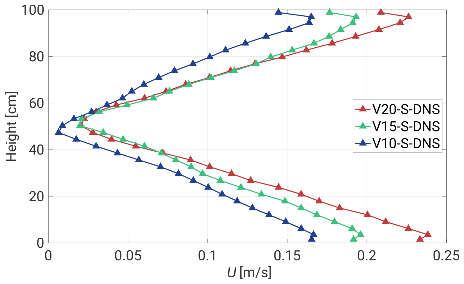
Figure C1 Magnitude of the mean velocity U profile near the axis of the chamber with respect to its height. Each curve represents a different ΔT.

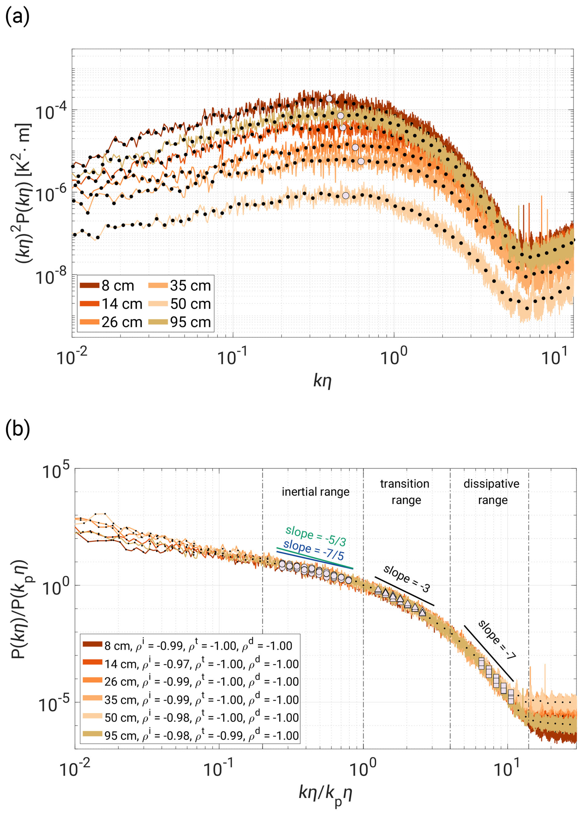
Figure C2 Analogous to Fig. 8 spectra of the V20-S-L case but in the wavenumber coordinate. (a) Scaled spectrum of kη²P(kη). (b) PSD $P\left(k\mathit{\eta }\right)/P\left(k_{\mathrm{p}}\mathit{\eta }\right)$ versus $k\mathit{\eta }/k_{\mathrm{p}}\mathit{\eta }$ with three defined regimes: inertial range (circles, $\mathrm{0.2}⩽k\mathit{\eta }/k_{\mathrm{p}}\mathit{\eta }⩽\mathrm{1}$), transition range (triangles, $\mathrm{1}⩽k\mathit{\eta }/k_{\mathrm{p}}\mathit{\eta }⩽\mathrm{4}$), and dissipative range (squares, $\mathrm{4}⩽k\mathit{\eta }/k_{\mathrm{p}}\mathit{\eta }⩽\mathrm{20}$). The legend includes the Pearson correlation coefficients p.

The first step of the scaling procedure involves the following transformations:

$$\begin{array}{ll}{\displaystyle }& {\displaystyle }k\approx \stackrel{\mathrm{̃}}{f}=f\left(\mathrm{2}\mathit{\pi }\right)/U,\\ {\displaystyle }& {\displaystyle }P\left(k\right)\approx P\left(\stackrel{\mathrm{̃}}{f}\right)=P\left(f\right)U/\mathrm{2}\mathit{\pi },\end{array}$$

where $P\left(\stackrel{\mathrm{̃}}{f}\right)$ and $\stackrel{\mathrm{̃}}{f}$ represent the scaled frequency spectrum and the scaled frequency, respectively. The DNS data revealed a symmetrical profile of the mean velocity U near the axis (see Fig. C1). It gradually decreases towards the bulk region, reaching about 0.02 m s⁻¹, and maintains approximately equal values near both plates. The resulting wavenumber spectral curves are rescaled with U and shifted accordingly. To collapse them, we found the Kolmogorov length scale, defined as $\mathit{\eta }=\left(\mathrm{2}\mathit{\pi }\right)/k_{\mathrm{n}}$ where k_n is the wavenumber noise level, and performed another scaling to obtain the P(kη) spectrum. The last step follows the procedure adopted by Zhou and Xia (2001).

In Fig. C2a, we present the estimation of k_pη, which is a direct analogy to f_p in Sect. 3.2 for the V20-S-L case in the scaled kη²P(kη) spectrum. Unlike the corresponding plot in the frequency domain (see Fig. 8a), k_pη does not oscillate around one value. Here, we observe a gradual increase in k_pη values towards the bulk region, with the kη²P(kη) maximum occurring around k_pη≈0.5. Figure C2b provides the final result of the frequency for wavenumber scaling. Both the slopes and dynamic ranges are conserved, providing a clear analogy to Fig. 8.

Appendix D: Standard deviation scaling

To verify whether and where we can observe thermal plume dominance in the chamber, we followed the methodology outlined by He and Xia (2019). They demonstrated a strong connection between plumes and the logarithmic root mean square temperature profile using a different setup, which consisted of water as a working fluid (Pr=4.34), a rectangular-shaped container with Γ=4.2, and Ra values from 3.2×10⁷ to 2×10⁸. For our purposes, we analyzed the standard deviation ${\mathit{\sigma }}_{T^{\prime }}$ distribution of the 19 min, 3 min, and DNS datasets. Figure D1 presents the results for two regions in the semi-log domain – ∼15–35 cm near the floor (Fig. D1a) and ∼65–95 cm near the ceiling (Fig. D1b). In both regimes we provided the respective Pearson correlation coefficients and fitted the curves for the 19 min time series.

Each profile in the lower half of the chamber exhibits a significant linearity correlation in the given region, including the 3 min experimental dataset. Only the V10-S case differs notably from the remaining results, dropping to $p=-\mathrm{0.59}$. The corresponding area in the upper half gives similarly high indications of the p values, excluding shorter measurements, providing evidence of a weaker thermal plume response. This observation is reasonable considering the previous discussion in Sect. 3.1 on differences between both regions of the cell.

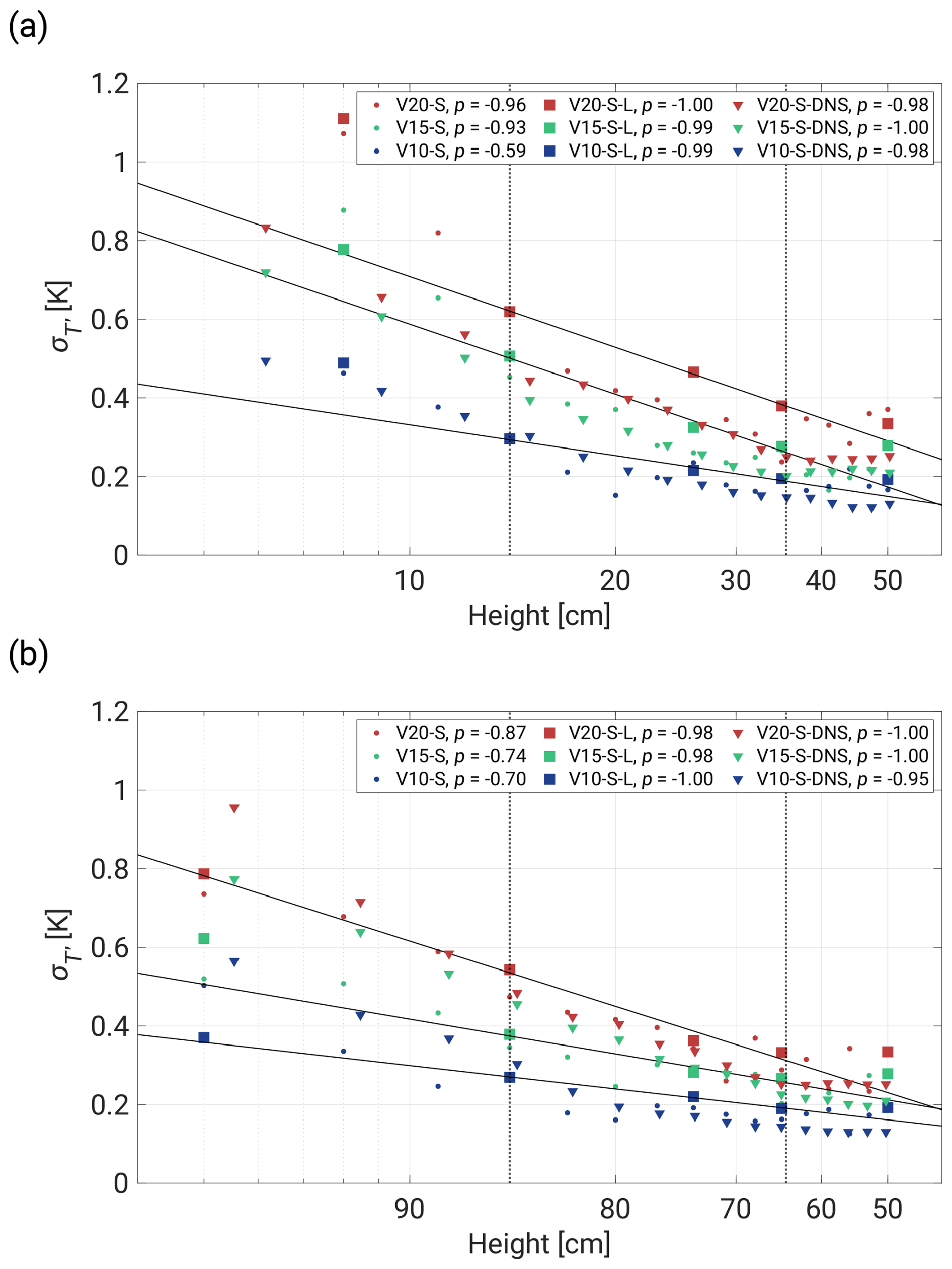
Figure D1 Standard deviation ${\mathit{\sigma }}_{T^{\prime }}$ distribution of the 19 and 3 min and the DNS dataset in the semi-log coordinate near the floor (a) and close to the ceiling (b). Both legends include Pearson correlation coefficients. Note that the fitted curves correspond only to the 19 min measurements.

It is worth mentioning that the zones outside the selected profiles are clearly dominated by different types of forces, resulting in very local dynamics in the RBC.