Assessment of horizontally oriented ice crystals with a combination of multiangle polarization lidar and cloud Doppler radar

The orientation of ice crystals plays a significant role in determining their radiative and precipitating effects; horizontally oriented ice crystals (HOICs) reflect up to ∼40 % more shortwave radiation back to space than randomly oriented ice crystals (ROICs). This study introduces an automatic range-resolved algorithm for HOIC identification using a combination of ground-based zenith-pointing and 15° off-zenith-pointing polarization lidars. The lidar observations provided high-resolution cloud-phase information. The data were collected in Beijing over 354 d in 2022. A case study from 13 October 2022 is presented to demonstrate the effectiveness and the feasibility of the detection method. The synergy of lidars and collocated Ka-band cloud radar, radiosonde, and ERA5 data provides phenomenological insights into HOIC events. While cloud radar Doppler velocity data allowed the estimation of ice crystal size, Reynolds numbers, and turbulent eddy dissipation rates, corresponding environmental and radar-detected variables are also provided. HOICs were present, accompanied by weak horizontal wind of 0–20 m s⁻¹ and relatively high temperature between −8 and −22 °C. Compared to the ROICs, HOICs exhibited larger reflectivity, larger spectral width, a larger turbulent eddy dissipation rate, and a median Doppler velocity of about 0.8 m s⁻¹. Ice crystal diameters (1029 to 1756 µm for 5th and 95th percentiles) and Reynolds numbers (28 to 88 for 5th and 95th percentiles) are also estimated with the help of cloud radar Doppler velocity using an aerodynamic model. One interesting finding is that the previously found switch-off region of the specular reflection in the region of cloud base shows a higher turbulence eddy dissipation rate, probably caused by the latent heat released due to the sublimation of ice crystals in the cloud-base region. The newly derived properties of HOICs have the potential to aid the derivation of the likelihood of their occurrence in output from general circulation models (GCMs) of the atmosphere.

1 Introduction

It has been recognized in the presence of Reynolds numbers between 1 and 100 (Pruppacher and Klett, 1996) that falling ice crystals in the atmosphere can become quasi-horizontally oriented, only slightly deviating from the horizontal alignment due to wobbling movements. Frequently observed atmospheric optical phenomena (halos) including sun dogs (parhelia), light pillars (sun pillar, moon pillar), circumzenithal arcs, and circumhorizontal arcs require the presence of horizontally oriented hexagonal plates. Tangent arcs require horizontally oriented hexagonal columns (Liou and Yang, 2016; Saito and Yang, 2019). Both crystal types, in general described as horizontally oriented ice crystals (HOICs), can produce angle-dependent specular reflection for the incident light. The effect of that specular reflection defines the cloud radiative properties over large areas. In fact, regions with dominant HOICs can produce remarkable sunlight glints with much higher reflectance than the surroundings, as has been observed by low-Earth-orbit (Bréon and Dubrulle, 2004) and deep-space passive satellites (Marshak et al., 2017; Várnai et al., 2019; J.-Z. Li et al., 2019).

HOICs reflect more shortwave radiation into space compared to randomly oriented ice crystals (ROICs), up to 40 % more according to modeling studies (Takano and Liou, 1989), thereby significantly influencing the radiation balance (Klotzsche and Macke, 2006). Calculation shows oriented plates intercept roughly twice as much sunlight as the perfectly randomly oriented ones (Várnai et al., 2019). Stillwell et al. (2019) confirmed the significant radiation difference for HOICs and ROICs using a long-term ground-based dataset. Additionally, horizontal orientation increases the drag force from the atmosphere and thus slows the sedimentation speed of ice crystals, increasing the cloud lifetime and persistence in atmospheric models (Heymsfield and Iaquinta, 2000).

Mirror-like specular reflection also strongly influences lidar observations. When the incident light is perpendicular to the main facets of HOICs, very strong backscatter and nearly no depolarization (specular reflection at normal incidence does not rotate the plane of polarized light) are found for zenith-pointing lidar (nadir-pointing for the spaceborne lidar case). However, when the incident light is several degrees off perpendicularly to the surface of HOICs, a relatively weak backscatter and higher depolarization ratio are found for off-zenith-pointing lidar (off-nadir-pointing for the spaceborne lidar case). This angle-dependent characteristic is beneficial for distinguishing the HOICs from ROICs (He et al., 2021a, b; Seifert, 2011). As another crucial feature, HOICs can lead to misclassification of the cloud phase based on the zenith/nadir polarization lidar-based cloud-phase discrimination due to the similarity of the near-zero depolarization ratios produced by both specular reflection from HOICs and backscattering from droplets of supercooled water cloud. To avoid specular reflection from HOICs, spaceborne lidars positioned several degrees off-nadir capture the cloud-phase information better, 3° for ATLID (Atmospheric Lidar) on board EarthCARE (Earth Cloud, Aerosol and Radiation Explorer) and CALIOP (Cloud-Aerosol Lidar and Infrared Pathfinder Satellite Observations) and 2° for ACDL (Aerosol and Carbon dioxide Detection Lidar) on board DQ-1 (Wehr et al., 2023; Hu et al., 2009; Dai et al., 2024). Many ground-based lidars and ceilometers have also been positioned several degrees off-zenith to reduce the HOIC contamination of supercooled-liquid-droplet identification schemes (e.g., Engelmann et al., 2016).

Despite its importance, limited knowledge exists regarding HOICs. Due to the perturbation of ice orientation by the detector, it is very difficult to use airborne in situ methods to measure the ice orientation. Remote sensing methods, including both ground-based measurement and spaceborne observations, have been developed and employed to investigate the characteristics of HOICs. Diattenuation, a polarization-dependent measure of scattering efficiency shown by oriented particles at so-called oblique angles, was proposed by Neely et al. (2013) for the study of HOICs and their radiation effects in Greenland (Stillwell et al., 2019). Seifert (2011) used zenith-pointing polarization Raman lidar to retrieve the lidar ratio of HOICs and pointed out that HOICs show a lower lidar ratio than supercooled water clouds. Westbrook et al. (2010) used the ratio of backscatter (color ratio) from an off-zenith-pointing ceilometer and a zenith-pointing Doppler lidar to identify and study HOICs, though their study lacked depolarization ratio capacity. He et al. (2021a), with a 30° off-zenith lidar along with a zenith-pointing lidar, used enhanced volume depolarization from off-zenith-pointing lidar as a feature to identify HOICs and found the horizontal orientation can form from a continuously descending ice cloud layer. However, they did not use the backscatter as a restraint and their identification method was manual. CALIOP separated HOICs from ROICs and liquid water cloud based on a layer-integrated attenuated backscatter and depolarization ratio threshold (Hu et al., 2009). With its global coverage, CALIOP shows a powerful advantage in observing the global distribution of HOICs. However, lidar attenuation when a liquid-water-topped cloud exists could lead to an underestimation of the HOICs fraction. The relatively coarse spatial resolution and layer-integrated, vertically homogeneous (within a determined cloud layer) official cloud-phase classification (Hu et al., 2009) are not detailed enough to investigate the horizontal orientation. The spaceborne lidar is more suitable for global-scale statistics, providing only a snapshot observation, which cannot observe the process-level evolution of HOICs. Passive satellites using glint to identify HOICs can provide the macroscopic distribution of oriented ice (Marshak et al., 2017; Bréon and Dubrulle, 2004) but without height-resolved information.

Fundamental questions about, for example, the frequency of HOICs still persist, and the literature provides different results as a consequence of the variability in the underlying detection and counting methods: profile-based (Ross et al., 2017), range-bin-based (Westbrook et al., 2010; Sato and Okamoto, 2011), cloud-layer-based (Zhou et al., 2012a; Saito et al., 2017), or area-based (Bréon and Dubrulle, 2004; Marshak et al., 2017). Westbrook et al. (2010) point out that many of the results from different studies are inconsistent. Noel and Chepfer (2010) found, using nadir-pointing CALIPSO (see Appendix F for further definitions of some of the abbreviations and symbols used in this paper) data, that 6 % optically thin ice cloud contains oriented ice. Zhou et al. (2012b) estimated HOICs exist in approximately 60 % of optically thick ice and mixed-phase cloud layers. Marshak et al. (2017) pointed out that roughly every third DSCOVR/EPIC image (see http://epic.gsfc.nasa.gov, last access: 29 July 2025) shows sunglint over land, which is most likely due to HOICs. The automated algorithm proposed in this paper can serve as a good starting point for future HOIC frequency and percentage studies.

More observations with HOIC identification capabilities are needed to improve the assignment of the orientation of ice hydrometeors in cloud parameterization schemes, which is usually not considered in current general circulation models or radiative transfer models (Klotzsche and Macke, 2006; Zhou et al., 2012b). Due to the latitude-dependent HOIC occurrence (Noel and Chepfer, 2010), long-term observation at midlatitude stations like Beijing (116.3° E, 40.0° N), China, is essential to help understand the orientation phenomenon.

Previous ground-based statistics are mostly case studies describing areas with specular reflection effects, lacking precise height-resolved bin-level observations and products. Compared to spaceborne observations, the ground-based dual-angle lidar scheme has a higher spatial and temporal resolution to analyze the evolution of HOICs, which is beneficial to our understanding of the process. It gives us a more comprehensive understanding of the environmental characteristics of the emergence of HOICs. In addition, simultaneous cloud radar observations, which very few HOIC studies utilized so far, can obtain Doppler velocities, which help us to estimate ice crystal size information and to derive turbulence information that helps to understand under which conditions HOICs tend to form.

Simultaneous observations using ground-based zenith and 15° off-zenith-pointing polarization lidars along with cloud radar (see Fig. 1) were conducted to study HOICs in Beijing, China, over 354 d in the year 2022. This article proposes an automatic algorithm for HOIC detection based on dual-angle polarization lidar observations and then explores the potential of such a unique system using collocated cloud radar, radiosonde, and ERA5 data. The article is structured as follows. Section 2 presents the instruments and data used. In Sect. 3, we detail the methodology employed to detect the cloud bins and then identify HOICs. Next, a case study is shown in Sect. 4. Finally, conclusions are drawn in Sect. 5.

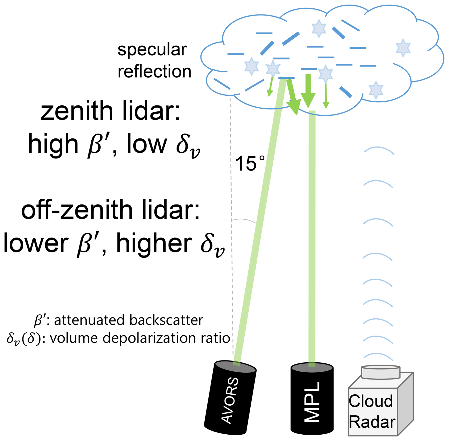
Figure 1 Schematic figure of the two lidars and the zenith-pointing cloud radar that were used in the framework of this study.

2 Instruments and data

We propose a new and unique set of instruments to study HOIC occurrence and formation: 2 polarization lidars with different zenith angles and Doppler cloud radar. The depolarization ratio measured by the zenith-pointing Micro Pulse Lidar (MPL) and 15° off-zenith-pointing AVORS lidar was calibrated using well-calibrated Raman lidar as a reference, as is described in detail in Appendix B2.

2.1 MPL

The Micro Pulse Lidar (MPL; model MPL-4B-IDS-532-AT) manufactured by Sigma Space Corporation has been continuously operated since 2016 (Chu et al., 2019; Xu et al., 2020; Chang et al., 2021) at the zenith angle on the roof of the Peking University (PKU) Physics Building (116.3° E, 40.0° N; ∼40 m above sea level). The temporal and vertical resolution of the MPL is 15 s and 15 m, respectively, and the blind zone is 195 m (Welton and Campbell, 2002). The pulse repetition frequency is 2500 Hz, and the pulse energy is 6–8 µJ. The MPL is a single-wavelength (532 nm) elastic polarization lidar with a field of view (FOV) of 0.1 mrad. Using the actively controlled liquid crystal retarder (LCR), the MPL achieves polarization detection capabilities with only one detector for the two polarization channels (Flynna et al., 2007). The MPL was placed in a container with air conditioning to maintain stable observations. On top of the container, there is a slightly tilted glass to guarantee that lidar observations are not interrupted by bad weather. A lens hood above the glass reduces the sunlight noise. Maintenance staff carefully wipe the glass above the lidar container every day to minimize attenuation caused by rain and aerosol deposits. Unless otherwise stated, the time in the paper is local time (LT, UTC+8).

2.2 AVORS lidar

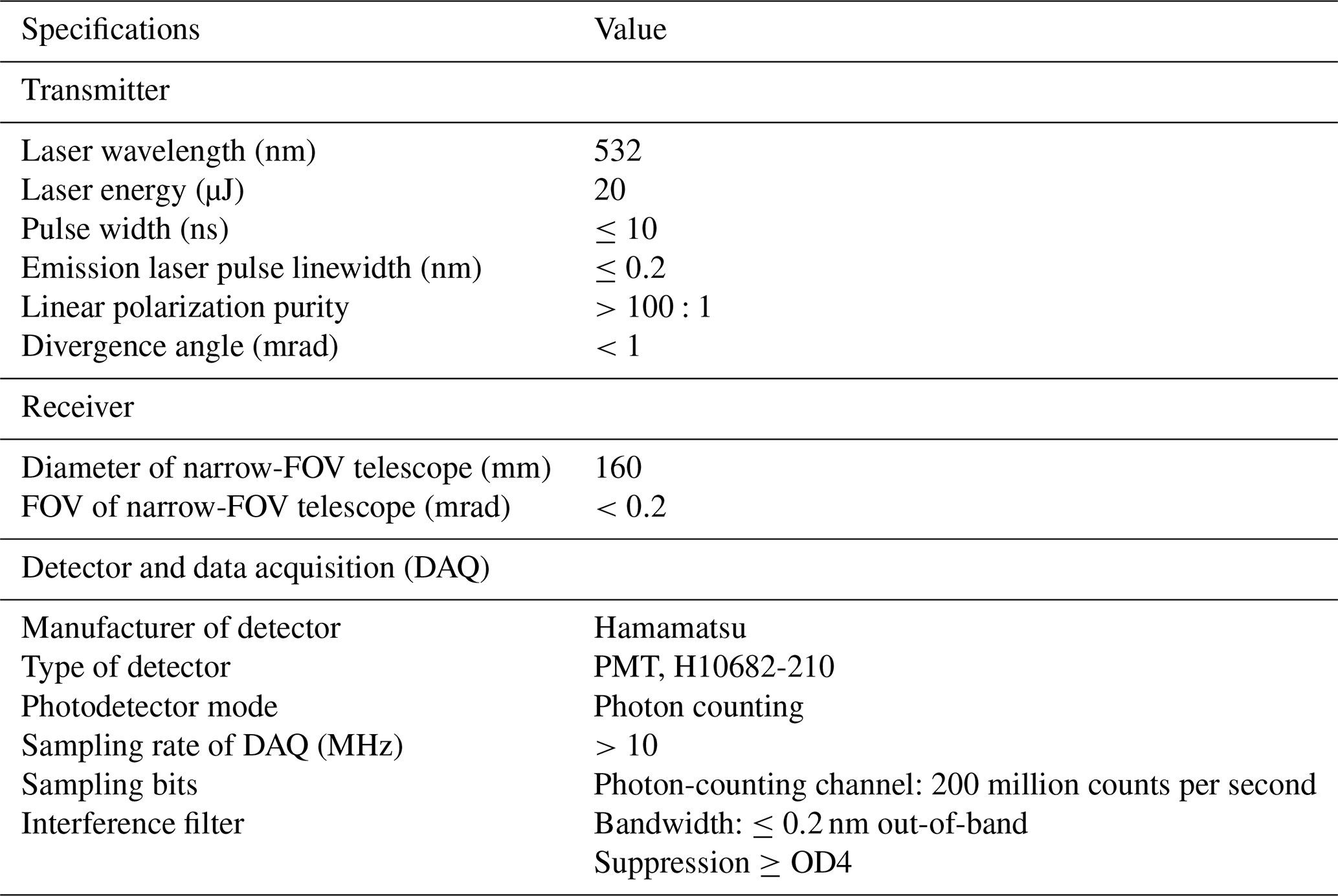
An off-zenith-pointing lidar (Portable Particle Lidar, http://en.avorstech.com/product/670.html, last access: 29 July 2025) manufactured by AVORS Technology has been continuously operating since 2022 (Sun et al., 2024). The AVORS lidar was placed 5 m away from the MPL on the same roof. The AVORS lidar is a single-wavelength (532 nm) elastic polarization lidar, with a rotatable base and an electric motor to change its zenith and azimuth angle. The laser beam of the AVORS lidar was placed 15° off the zenith (towards the north to reduce the possible sunlight noise to the greatest extent) to avoid specular reflection during our study. The pulse energy is 20 µJ with a pulse repetition frequency of 2500 Hz, and the FOV of the telescope is 0.2 mrad. The temporal and vertical resolution of the AVORS lidar data is 10 or 60 s (adjustable, most of the time 60 s in this research) and 15 m, respectively, and the blind zone is 45 m. Technical specifications of the lidar system are listed in Table A1. Note that the AVORS lidar has two photomultiplier tube (PMT) detectors for each polarization channel (Fig. A1). In the following analysis, the height of observations from the AVORS lidar was calculated as $\text{cos}\left(\frac{\mathit{\pi }}{\mathrm{12}}\right)$ times the range from the lidar. The AVORS lidar was installed outdoors, and the temperature was maintained by its own air-conditioning system integrated inside the lidar. Due to the lack of containers or lens hoods, the lidar signal is slightly more contaminated by sunlight noise in the daytime, resulting in a relatively low signal-to-noise ratio (SNR). Furthermore, the AVORS lidar was zenith-pointing from 9 May to 3 June 2023; during this period the depolarization ratio for cloud could be compared with that of the MPL (Fig. B3).

The uniqueness of the 15° off-zenith angle observation is valuable in this research. Previous research shows that the 3° off-nadir angle of CALIOP was not sufficient to completely eliminate the effects of specular reflections (Noel and Chepfer, 2010; Kikuchi et al., 2021); hence CALIOP possesses the ability to offer a product about oriented ice at the 3° off-nadir angle. Also, ground-based polarization lidar with a 4 or 5° off-zenith-pointing angle can also sometimes show specular reflections (Tansey et al., 2023; Seifert et al., 2011). The 30° off-zenith angle of He et al. (2021a) is too large, and there will be a large horizontal offset at high altitude. In this study, a 15° off-zenith angle is a moderate angle, avoiding the backscatter specular reflection of HOICs as much as possible and also trying to ensure that the same cloud can be seen by both lidars.

2.3 Raman lidar

Portable, eye-safe lidars, such as MPL and AVORS, have polarization capabilities. Preliminary results revealed that the calibration of the systems needs to be improved in order to make the collocated measurements comparable. A well-characterized lidar was used as a reference to characterize the two micropulse lidar systems. A Raymetrics Raman lidar (model LR231-D300) at the same campus (about 360 m away from MPL and the AVORS lidar) was employed as the reference for the depolarization ratio (Li et al., 2016; J. Li et al., 2019; Tan et al., 2019, 2020a, b; Ren et al., 2021). The Raman lidar operates at three wavelengths (355, 532, and 1064 nm); two of them – 355 and 532 nm – are equipped with polarization channels. In the present study, the 532 nm channel of this Raman lidar has been designated as a reference for the calibration of the depolarization ratios of the other two lidars (see Appendix B2 for detail). Its performance of depolarization measurement has been verified by several previous studies (Tan et al., 2020a, b). The Δ90 method was employed to ensure its accuracy in terms of the depolarization ratio (Freudenthaler et al., 2009). Note that we do not use this Raman lidar for HOIC identification due to its discontinuous observation.

2.4 Cloud radar

To further explore the potential of the new approach in the investigation of HOIC events, additional information from a radar instrument was considered. The larger wavelength of the radar instrument makes it able to penetrate deeper into clouds compared to lidar; it is also more sensitive to large hydrometeors. The Doppler spectrum provides an estimation of the falling velocity of particles, which allows us to estimate the particle size using aerodynamic models. The radar measurements were also used to derive turbulence-related information, such as the turbulent eddy dissipation ratio (EDR) and Reynolds number (see Appendix D and E), which may play a significant role in the orientation of ice crystals. To our best knowledge, no Doppler cloud radar data have been used to investigate the identified horizontally oriented ice except for in Westbrook et al. (2010) and Stillwell et al. (2018), so our approach provides a unique chance to investigate more radar-based characteristics for different orientation behaviors of ice crystals.

A 33.44 GHz, Ka-band, solid-state, depolarization, multi-mode, zenith-pointing millimeter-wave cloud radar (MMCR, model HMB-KP) manufactured by the Beijing Institute of Radio Measurement has been continuously operating at Peking University since 2018 (Wang et al., 2022; Zhang et al., 2024). The cloud radar is placed 5 m away from the MPL container. The temporal resolution is about 13 s (adjustable), and the vertical resolution is 30 m. The radar operates in four alternating modes: boundary layer mode (mode 1), cirrus mode (mode 2), precipitation mode (mode 3), and middle-level mode (mode 4) (Ding et al., 2022). These four modes vary in pulse compression ratios and numbers of both coherent and incoherent integrations. The boundary layer mode is designed to identify low-altitude clouds by utilizing a narrower pulse waveform and increasing the number of coherent integrations to enhance detection capability. In the cirrus mode, pulse compression techniques are employed to boost sensitivity for detecting high-altitude clouds with weaker radar echoes. The precipitation mode features an extended unambiguous range and velocity measurements tailored for observing rainfall. The middle-level mode similarly applies pulse compression techniques but with a reduced number of coherent integrations. Furthermore, there is one combined mode (mode 8) that combines all the modes to produce one final observation result, which we use in this research. The radar measurements contain raw data of Doppler spectra and spectral moments including reflectivity, mean Doppler velocity, spectrum width, and the linear depolarization ratio. The minimum detectable reflectivity factor of this radar is −40 dBZ. Compared to lidars, radar exhibits greater sensitivity to larger particles (Westbrook et al., 2010; Bian et al., 2023). However, this Ka-band cloud radar may fail to detect certain tiny liquid droplets and optically thin ice clouds.

2.5 Radiosonde and ECMWF ERA5 reanalysis data

Radiosondes were launched every day at 00:00 UTC (08:00 LT) and 12:00 UTC (20:00 LT) at the Beijing Nanjiao meteorological site (116.47° E, 39.80° N; WMO no. 54511), 25 km from our lidar site (Chu et al., 2019), providing meteorological parameters, e.g., temperature, relative humidity, and horizontal wind speed and direction. As a measure to compensate for the time sparsity of the radiosonde, ECMWF ERA5 reanalysis from the grid point of PKU (116.3° E, 40.0° N) was used to provide the meteorological parameters, i.e., the temperature, wind, and relative humidity over ice. ERA5 reanalysis data for 2022 were compared with simultaneous radiosonde profiles, as in Yin et al. (2021), and the differences in temperature, wind speed, and relative humidity are 0.2±0.86 °C, 0.53±1.98 m s⁻¹, and −5.46 %±12.69 %, respectively, indicating reliability of ERA5 data for our analysis.

3 Methodology

This section introduces a new identification scheme and describes the analysis procedure. First, raw lidar data were calibrated to obtain the attenuated backscatter coefficient (see Appendix B1). Second, lidar, cloud radar, and ERA5 data were re-gridded (averaged or interpolated) to 5 min × 15 m resolution. Then the following algorithms and corrections were applied to get the HOICs and other hydrometeor types.

3.1 Cloud-layer identification algorithm

An advanced value distribution equalization method (Zhao et al., 2014) was applied to identify cloud bins from lidar backscatter signals. Next, the overlap region of the cloud bins detected by both the MPL and the AVORS lidars was selected for the further cloud-phase determination algorithm. For HOIC cases, zenith-pointing lidar observations have a much stronger backscatter than off-zenith-pointing lidar observations. The identification of cloud bins mainly depends on the backscatter; the cloud detection algorithm can identify at least one range bin as a cloud when the backscatter of the bins reaches a predefined threshold, whose determination is explained by Zhao et al. (2014). The limitation of the cloud detection algorithm to those regions where the signals of both lidars overlap will lead to an underestimation of some upmost HOIC range bins (beyond the off-zenith lidar attenuation region but still clear in zenith lidar observation; compare Fig. 4a, c, and g).

It is essential to evaluate whether the two lidars detect the same cloud layer by estimating the typical horizontal deviation of the two laser beams at cloud height. For a cloud at an altitude of 6 km, the horizontal deviation from the zenith-pointing lidar is 6 km × $\tan \left(\frac{\mathit{\pi }}{\mathrm{12}}\right)=\mathrm{1.6}$ km. Assuming a horizontal wind speed is v=20 m s⁻¹ (see Fig. 6b) and the wind direction is along the line between the scattering volumes of the two-angle lidars, the horizontal movement of the cloud is 6000 m within 5 min, which is the temporal resolution utilized in data processing. Consequently, if both lidars observe the same cloud within the same time slot (>5 min), the horizontal deviation of the off-zenith-pointing lidar is less significant (1.6 km < 6 km), although with increasing height, the horizontal distance between the probed volumes also increases (from 0.268 km at 1 km height to 2.68 km at 10 km height). In reality, the wind direction does not always align with the line connecting the scattering volumes of the two-angle lidars. Therefore, we must assume horizontal homogeneity of the detected cloud layers over a certain lateral scale. This assumption is likely valid for horizontally homogeneous stratiform clouds. However, caution is needed for discrete, small-scale clouds, as misalignment may occur.

3.2 Cloud-phase determination algorithm

A specialized algorithm (Fig. 2) is applied to differentiate between different cloud phases for the intersecting cloud bins observed by both lidars. First, we utilized the temperature of homogeneous nucleation ($<-\mathrm{38}$ °C) to distinguish the ice phase, followed by using the off-zenith-pointing lidar volume depolarization ratio of 0.1–0.3 to identify ice-containing cloud bins at temperatures between 0 and −38 °C. Cloud bins with a volume depolarization ratio of ≥0.3 are categorized as randomly oriented ice crystals (ROICs). Cloud bins with a volume depolarization ratio of 0.1–0.3 are categorized as mixed-phase cloud (MPC) bins. If the cloud parts categorized as ROICs or MPC bins have δ_off-zenith>0.1 and δ_zenith<0.1, then we used a zenith-to-off-zenith ratio of attenuated backscatter >2 and a zenith-to-off-zenith ratio of the volume depolarization ratio <0.6 as stringent criteria to exclusively capture the most representative signals of HOICs, since the specular reflection effect is strong enough without ambiguity. On the contrary, ice-containing bins that do not meet the three thresholds are categorized as ROICs or MPC bins. It should be mentioned that the real case of the orientation of the ice crystals is always a mixture within a lidar-detected bulk (Saito and Yang, 2019; Borovoi et al., 2018). This means that the HOIC label indicates that the specific range bin contains HOICs (with a certain proportion) which produce an unambiguous specular reflection signal; however, some ROICs may still exist in the range bin.

The threshold values were fixed empirically from the whole cloud dataset collected during 2022 (Seifert, 2011; Lewis et al., 2020; Whitehead et al., 2024). The criteria used to select a typical HOIC bin are shown in Fig. 3. Figure 3a is the median volume depolarization ratio as a function of temperature for all detected cloud layers in 2022. The depolarization ratio δ indicates particle sphericity: ROICs show a higher volume depolarization ratio on the order of 0.3–0.5, while spherical liquid droplets have near-zero values (Ansmann et al., 2008; Seifert, 2011). A high depolarization ratio (>0.3) at temperatures below −38 °C (the threshold temperature for homogeneous freezing) and a low depolarization ratio (<0.1) at temperatures above 0 °C are identified as the depolarization ratio criteria for ice and liquid water clouds, respectively. The two depolarization ratio threshold values are shown with dashed red lines in Fig. 3a. Zenith lidar shows much lower depolarization than off-zenith lidar between −40 and 0 °C, probably due to contamination of the data by HOICs. Figure 3b shows the ratio of attenuated backscatter and depolarization ratio by means of a density scatterplot which is based on all cloud bins detected in 2022. Most cloud bins accumulate around the 1:1 line, indicating that zenith lidar and off-zenith lidar have a comparable volume depolarization ratio and comparable attenuated backscatter. In contrast, a distinct tail-like cluster is evident in the upper-left region of Fig. 3b. The lower depolarization and higher backscatter in zenith lidar observations compared to off-zenith lidar observations shown in this cluster are clear features of HOICs. For the identification scheme, we use a zenith-to-off-zenith ratio of the attenuated backscatter ratio greater than 2 and depolarization ratio less than 0.6 as criteria to avoid the most frequent cloud bins (green, yellow, and red) in the center part of Fig. 3b. These are relatively strict criteria as they consider both the criteria for both the attenuated backscatter ratio and the depolarization ratio to categorize the most representative bins for specular reflection. In the case of liquid water clouds, the zenith-to-off-zenith depolarization ratio differs from 1, ranging between 0.55 and 1 according to Jimenez et al. (2020) as the ratio of lidar FOVs is 1:2. However, the backscatter ratio will be less than 1, making the distinction of HOICs unambiguous with the described criteria.

Figure 3c shows the density scatterplot between the off-zenith lidar's attenuated backscatter and depolarization ratio. Two evident clusters can be found: a low depolarization ratio and high backscatter indicating liquid water clouds and a high depolarization ratio and low backscatter indicating ice clouds, respectively. Nonspherical ice crystals exhibit higher δ_v compared to spherical liquid water droplets, whereas droplets have higher β^′ due to their higher concentration. The dashed black lines (δ_v<0.1 and ${\mathit{\beta }}^{\prime }>\mathrm{5}$ Mm⁻¹ sr⁻¹) indicate the criteria for the classification of liquid water. If a cloud bin meets the two introduced criteria and has a temperature ≥0 °C, it is categorized as liquid water (or water as an abbreviation). If the temperature is below 0 °C, it is then flagged as a supercooled liquid water cloud (SWC). Note that if a cloud bin has a relatively low depolarization ratio (δ_v<0.1) but does not meet the attenuated backscatter criterion (${\mathit{\beta }}^{\prime }\le \mathrm{5}$ Mm⁻¹ sr⁻¹), it is classified as a non-typed cloud bin (similar to Baars et al., 2017). This usually happens when the concentration of cloud particles is low or the range bins are actually some dense aerosol particles (e.g., mineral dust). Discriminating optically thin clouds and dense aerosol is still a challenge for a cloud mask algorithm based on lidar backscatter signal; thus we exclude the non-typed cloud bins from further analysis in this study.

Figure 2 Flowchart of the algorithm for the classification of hydrometeor types.

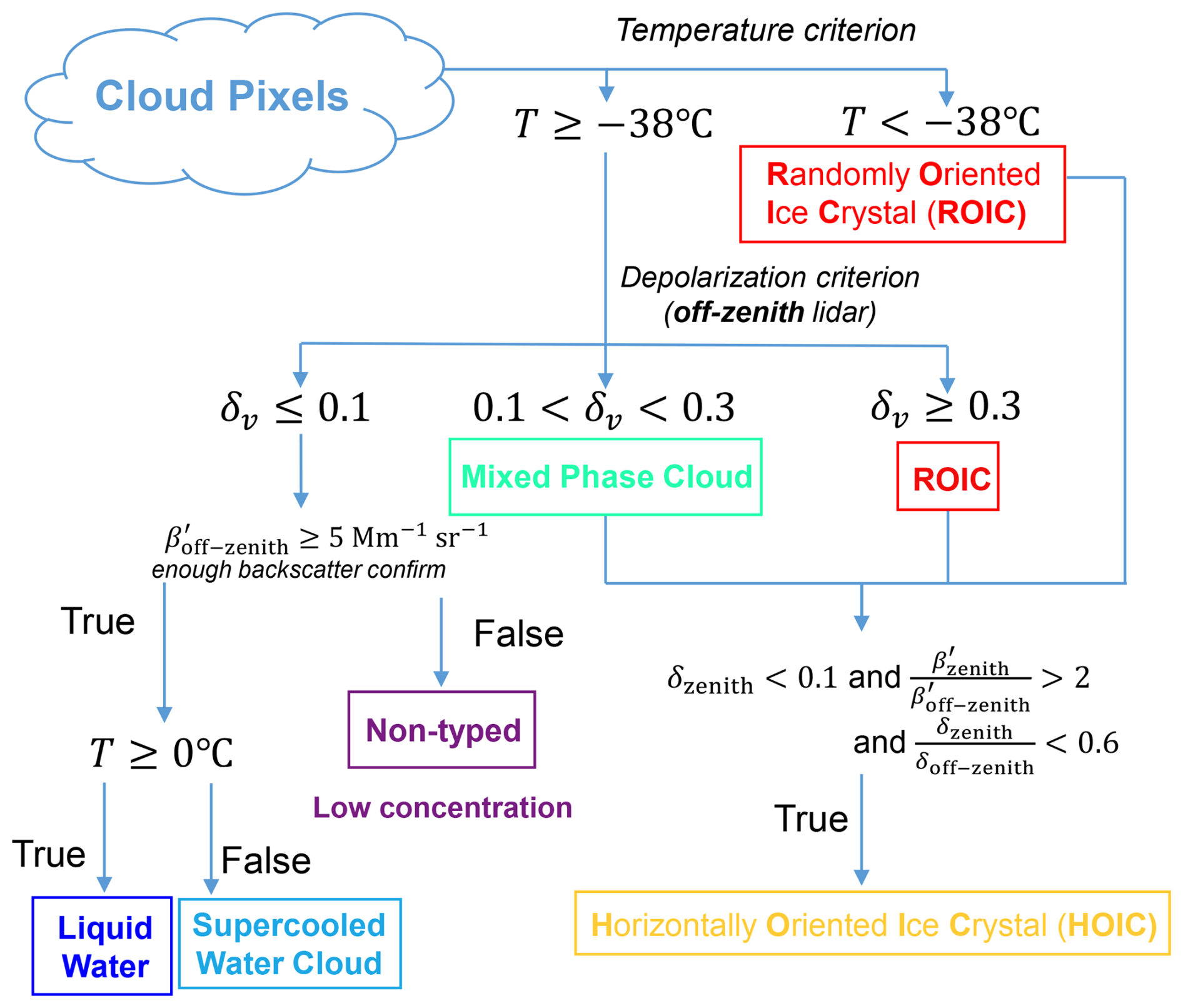
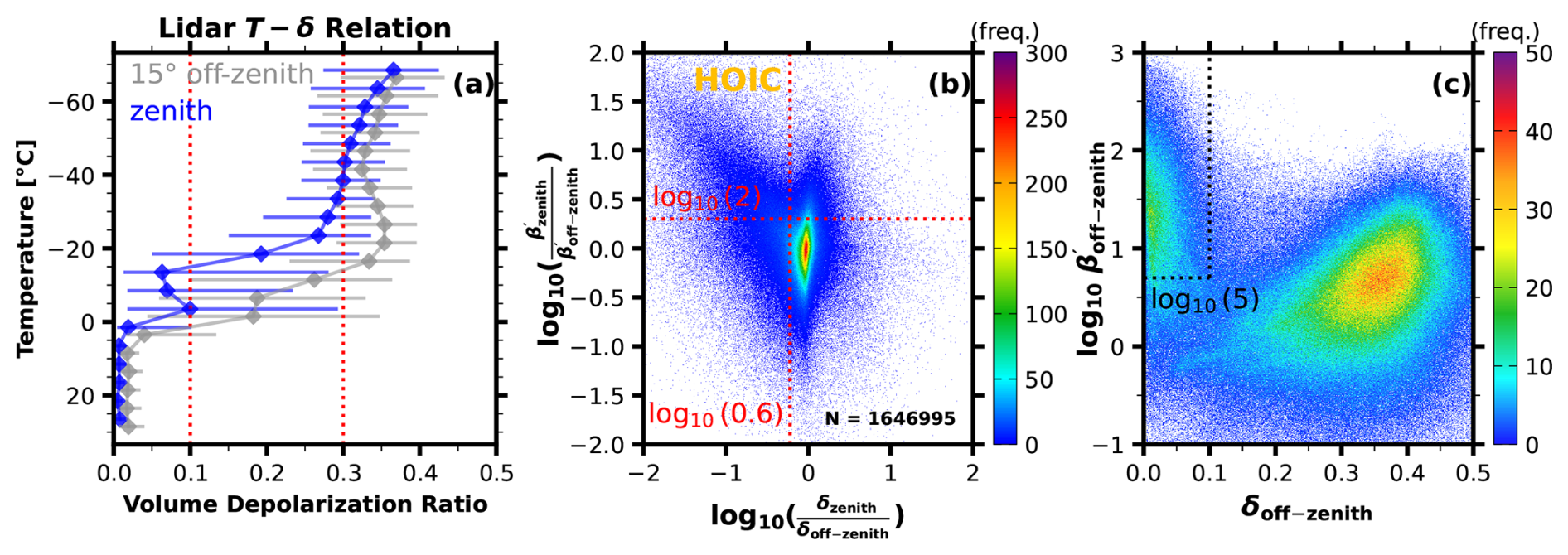
Figure 3 Definition of criteria for identification of the HOICs (dashed red lines). All subfigures were created using all the cloud bins observed in 2022. (a) The median volume depolarization ratio as a function of temperature for each height bin within all detected cloud bins in temperature increments of 5 °C. Horizontal bars indicate the interquartile range (IQR). (b) Density scatterplot of the ratio of zenith-pointing to off-zenith-pointing lidar volume depolarization and attenuated backscatter, log₁₀ scale. (c) Density scatterplot of volume depolarization ratio and attenuated backscatter (in Mm⁻¹ sr⁻¹, log₁₀ scale) for off-zenith-pointing lidar. Dashed black lines indicate the criteria used for the identification of liquid water.

3.3 Cloud-phase correction

After applying the cloud-phase discrimination algorithm, the potential multiple-scattering effects and the contamination of the molecular depolarization ratio for ice clouds have to be considered; thus the following two corrections were conducted.

3.3.1 Typing correction above liquid layers

The off-zenith lidar, with its greater FOV (0.2 mrad compared to 0.1 mrad), generally results in a higher depolarization ratio at the top of water clouds than the zenith-pointing MPL (see Fig. 3a, T>0 °C region). This occurs when the effect of multiple scattering is pronounced as it penetrates the water cloud. Due to the different dead time reactions for the two lidar detectors, MPL shows stronger attenuated backscatter at low altitudes (<1.2 km). We thus categorized HOIC bins below 1.2 km as liquid water cloud (T≥0 °C) or supercooled liquid water cloud (T<0 °C). For water clouds above 1.2 km, if the topmost 100 m of a profile has been flagged as HOICs but the layer shows liquid water towards the bottom, the upper bins will be classified as liquid water. This criterion allows us to exclude possible artifacts caused by horizontal homogeneities and strong attenuation of the laser beam in the liquid cloud layer. In this way, this method conservatively corrects most misclassified HOICs at the top of water clouds back to the water phase.

3.3.2 Ice virga correction beneath pure ice clouds

As the elastic backscatter lidars we used for our study lack Raman or high-spectral-resolution channels, we use the volume depolarization ratio instead of the particle depolarization ratio to avoid the introduction of additional uncertainties by the assumption of lidar ratios in the Klett–Fernald method (Fernald, 1984) that would be required for calculation of the ratio of particle to molecular backscattering. However, application of the volume depolarization ratio introduces certain ambiguities within thin clouds or in presence of low concentrations of ice crystals, as is the case, e.g., in the ice virga region beneath pure ice clouds. The reason for this is that the magnitude of the volume depolarization ratio depends on the relative contribution of the molecular depolarization ratio, which is caused by backscattering by air molecules (Cairo et al., 1999). With the decreasing contribution of particle backscattering, the molecular backscattering and the associated low depolarization ratio of 0.004 (in the case of the AVORS lidar) contaminate the total signal and decrease the effective volume depolarization ratio of the ice crystals, resulting in the ice bin not reaching the depolarization ratio criterion of 0.3 for the off-zenith-pointing AVORS lidar. This leads to them being categorized improperly as mixed-phase cloud bins, even though actually no water droplet may exist under this circumstance. For MPC bins near the bottom of a cloud, the following procedure was thus applied. If more than 5 out of the 10 adjacent cloud range bins above an MPC bin contain ROICs and the temperature is below −20 °C, they are re-categorized as ROICs. The threshold of −20 °C is a typical criterion for the sharp decrease in the fraction of supercooled liquid water (Yorks et al., 2011; Wang et al., 2019), even though a small likelihood of there being liquid water persists down to −38 °C (see, e.g., Radenz et al., 2021, and Fig. 4g, 20:00 to 21:00 at heights above the −22 °C isotherm).

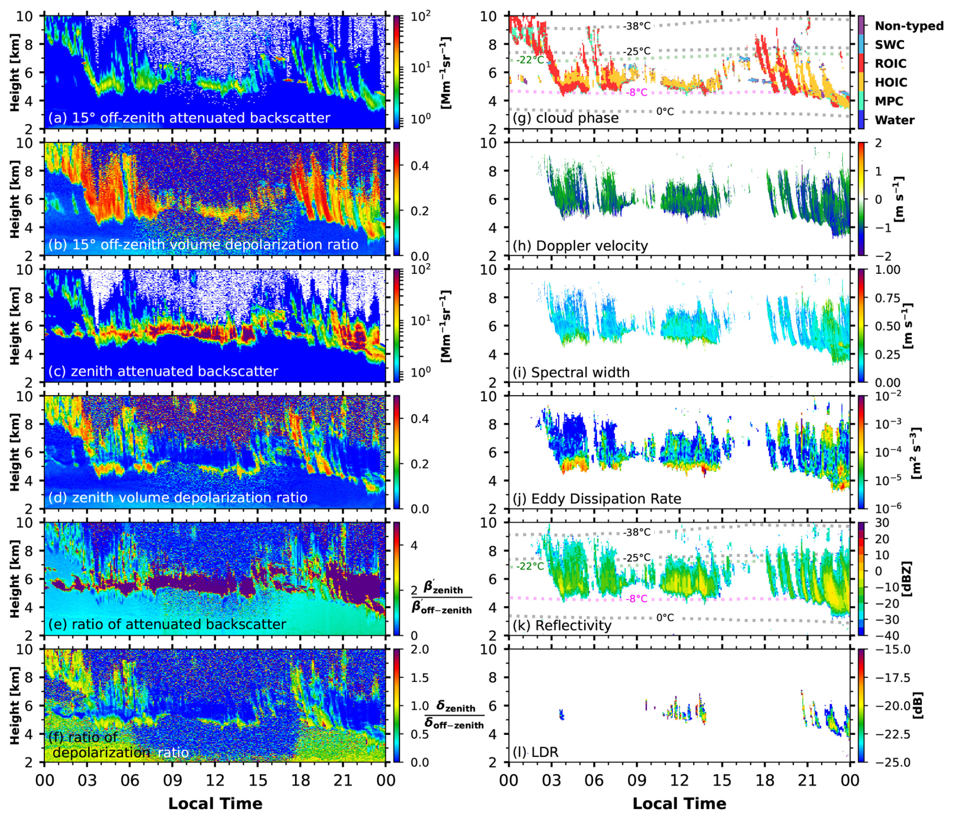
Figure 4 Lidar (a–g) and zenith-pointing Ka-band cloud radar (h–l) observations on 13 October 2022, time–height contour plots (5 min/15 m resolution for a–g, 13 s/30 m resolution for h and i to show the variation in Doppler velocity, 5 min/30 m for j–l). (a) The 15° off-zenith-pointing lidar attenuated backscatter. (b) The 15° off-zenith-pointing lidar volume depolarization ratio. (c) The zenith-pointing lidar attenuated backscatter. (d) The zenith-pointing lidar volume depolarization ratio. (e) The ratio of attenuated backscatter for zenith-pointing and off-zenith-pointing lidar. (f) The ratio of volume depolarization for zenith-pointing and off-zenith-pointing lidar. (g) Cloud-phase categorization results with isotherm from ERA5 data. Abbreviations of SWC, ROIC, HOIC, and MPC represent supercooled liquid water cloud, randomly oriented ice crystal, horizontally oriented ice crystal, and mixed-phased cloud. There is no cloud bin categorized as (warm) water due to the subzero temperature. (h, i, k, l) Cloud-radar-detected momentum data: Doppler velocity, spectral width, reflectivity (with isotherm from ERA5 data), and the linear depolarization ratio (LDR). (j) The cloud-radar-retrieved eddy dissipation rate (EDR, ϵ).

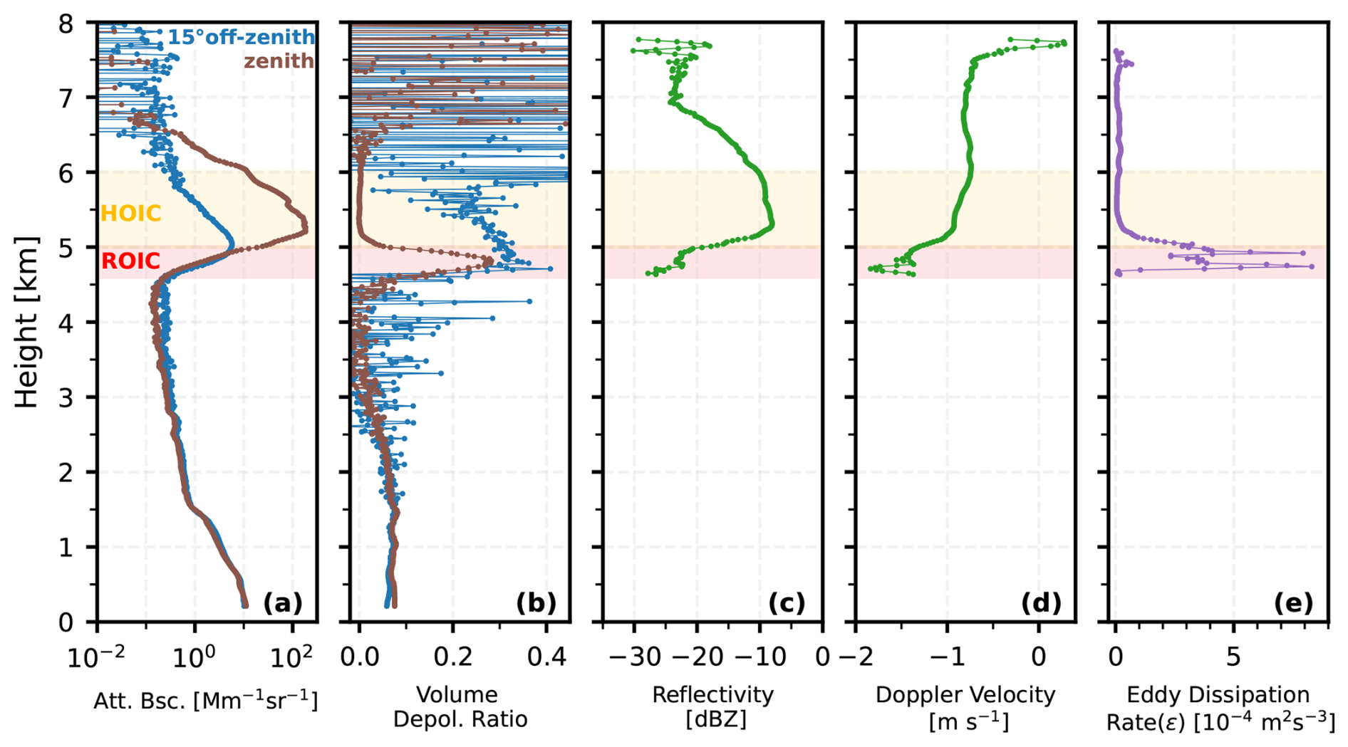
Figure 5 Lidar (a–b) and radar (c–d) observations at 11:00–12:00 on 13 October 2022; panel (a) shows the attenuated backscatter profiles from both zenith and off-zenith-pointing lidars; panel (b) shows the volume depolarization ratio from both lidars; panels (c) and (d) show the radar reflectivity and Doppler velocity, respectively. (e) The retrieved eddy dissipation rate. The orange-shaded regions denote the presence of HOICs, and the red regions represent the dominance of ROICs.

4 Case study on 13 October 2022

Figure 4 illustrates a case study of a mid-level cloud layer from 13 October 2022, when strong specular reflections were observed with the zenith-pointing lidar for almost the whole day. High backscatter and a low depolarization ratio in the zenith-pointing lidar observations and much lower backscatter and higher depolarization in the off-zenith-pointing lidar measurements indicated the presence of HOICs. The HOIC flag as derived by the algorithm introduced in this study is denoted in orange in Fig. 4g. Figure 5 shows average profiles of selected lidar and radar parameters for the period from 11:00 to 12:00 (LT) on 13 October 2022. The attenuated backscatter coefficient of HOICs (orange-shaded region) observed by zenith-pointing lidar is nearly 2 orders of magnitude larger than that observed by the off-zenith-pointing lidar (Fig. 5a). The volume depolarization ratio from the zenith-pointing lidar is nearly zero, while for the off-zenith lidar observation, the peak volume depolarization ratio exceeds 0.3 (Fig. 5b). Additionally, Fig. 5c and d, respectively, illustrate that the radar reflectivity factor is greater for HOICs, compared to ROICs, while the Doppler velocity is smaller.

This HOIC event persisted for nearly the whole day. Some HOIC bins showed strong attenuated backscatter for the zenith-pointing lidar but relatively low attenuated backscatter for the off-zenith-pointing lidar. Still, between 00:00 and 03:00 such bins were not identified as cloud, probably because the backscatter observed by the off-zenith-pointing lidar was too small for triggering the cloud mask detection for the off-zenith-pointing lidar. This demonstrates the stringency of the cloud identification criterion of the HOIC detection algorithm.

4.1 General description of a HOIC event

It is noteworthy that zenith lidar observations for some regions show a high depolarization ratio below the cloud levels of strong specular reflection. Prominent time–height regions where this was the case are, for instance, the time periods from 03:00–08:00 and from 11:00–15:00 at the height level of 4–5 km. This phenomenon is described as the “switch-off” of the specular reflection conditions (Westbrook et al., 2010; He et al., 2021a). Having the observations of both depolarization lidars and Doppler cloud radar available, this study aims to zoom in on this phenomenon in more detail than has been done in previous studies. The cloud radar observations (Fig. 4) show that the Doppler velocity changes significantly with time at the cloud base of the high-depolarization regions at the cloud base (compare Figs. 4d and h). The zenith lidar observation's high-depolarization-ratio region also coincides with a relatively high spectral width of Doppler velocity (Fig. 4i). A higher spectral width usually means stronger turbulence, more complex particle spectral distributions, stronger wind shear, beam broadening within the region, etc. (Kollias et al., 2007). In order to separate the effect of turbulence from other factors affecting spectral width, the turbulent eddy dissipation rate (EDR, ϵ) was computed to reflect the turbulence (Figs. 4j and 5e) using quantities including the standard deviation of Doppler velocity and horizontal wind speed. Details on the EDR retrieval are outlined in Appendix E. Measuring the turbulent kinetic energy (TKE) dissipation rate or turbulent eddy dissipation rate, which represents the rate of conversion of TKE into heat or the rate at which the TKE is dissipated by viscosity, is a good way to estimate the turbulence activity. As a quantitative proxy for atmospheric turbulence, a large EDR indicates rapid energy dissipation and high atmospheric turbulence (Griesche et al., 2020). The high-δ_v region above the cloud base (Fig. 5b, brown line within red-shaded region; see also Fig. 4d) in the zenith lidar observation has a higher eddy dissipation rate (Fig. 5e; see also Fig. 4j), suggesting that the strong turbulence may be linked to latent heat release from the sublimation of ice crystals near the cloud base. Another possible explanation is that this stronger turbulence in return causes the breakup of the ice crystal orientation. Horizontally oriented ice crystals need calm dynamic conditions and low turbulence to maintain their quasi-horizontal orientation (Klett, 1995; Garrett et al., 2015).

The following subsections analyze the environmental variables, cloud-radar-observed variables, and diameter and Reynolds numbers retrieved for HOICs. Then, the relationship between supercooled water clouds and the different orientations of ice crystals is discussed.

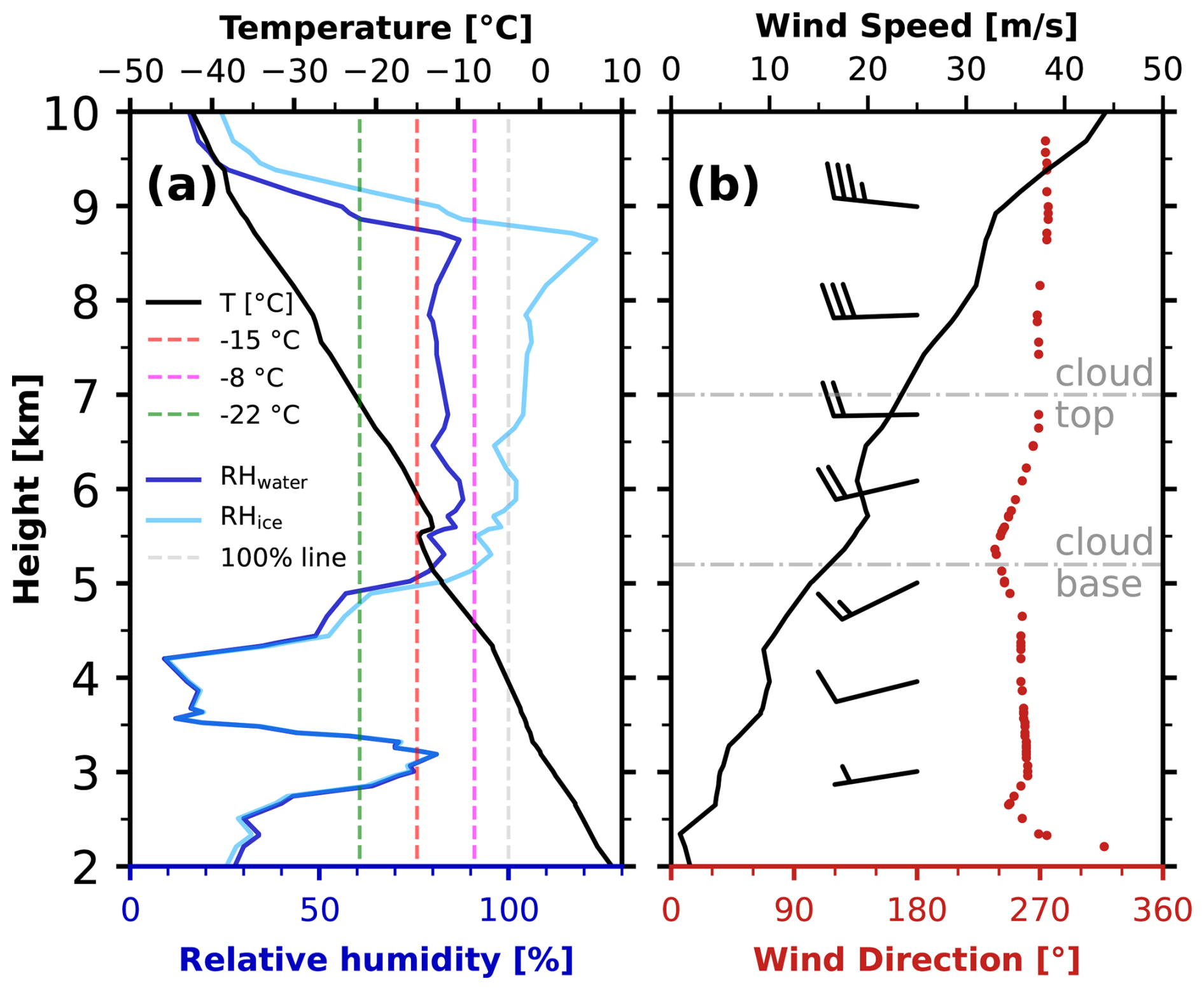
Figure 6 Beijing Nanjiao radiosonde profile (25 km away from PKU) at 08:00 LT (UTC+8) on 13 October 2022. (a) Temperature (black) and relative humidity with respect to liquid (deep blue) and ice (light blue) profiles; (b) wind speed (black), wind direction (red), and wind barbs. The two horizontal dash-dotted gray lines represent the cloud base, at approximately 5.2 km, and the cloud top, at around 7 km.

4.2 Environmental variables

Figure 6 shows the measurements of a radiosonde that was launched at Beijing Nanjiao station at 08:00 LT on 13 October, including the temperature and relative humidity, and the horizontal wind speed and direction profile. The temperatures of −8, −22, and −15 °C are denoted using dashed magenta, green, and light-red lines, respectively. Between temperatures of −8 and −22 °C, plate-like ice crystals tend to form, according to the ice crystal habit diagram, i.e., the morphology of ice crystals as a function of temperature (Libbrecht, 2005; Li, 2021; Bailey and Hallett, 2009). Overall, the highest probability of HOICs occurring was reported at the temperature level of −15 °C (Westbrook et al., 2010). In Fig. 6a, the temperature for typical specular reflection (between 5 and 7 km) is around −15 °C, which falls within the plate-like ice crystal temperature range of −22 to −8 °C, while the relative humidity over ice (Fig. 6a, light-blue line) approaches or slightly exceeds 100 %. As seen from Fig. 6b, the wind was westerly and relatively light (approximately 10–20 m s⁻¹) at the altitudes of the HOIC layer, which is beneficial for HOICs to maintain. Since the horizontal orientation is quasi-horizontal with some fluttering or a wobbling angle, an increase in horizontal wind speed may impinge upon the principal facet of the HOICs, generating significant torque that could potentially disrupt their orientation. Figure 6b also shows that the wind speed and direction of the cloud-base region (around 5.2 km) changed sharply along the different altitudes. This wind shear could induce turbulence in this region, thereby establishing conditions conducive to disrupting the horizontal orientation of ice crystals.

Figure 7 shows the normalized frequency of HOICs and ROICs under different horizontal wind speed and temperature conditions. It can be concluded that HOICs usually occur accompanied by smaller horizontal wind speeds and higher temperatures. Higher temperatures (−8 °C $>T>-\mathrm{22}$ °C) favor the formation of plate-like ice crystals, while weaker horizontal winds exert less torque to disturb their quasi-horizontal orientation. Additionally, Fig. 7c shows the density scatterplot of horizontal wind speed and temperature conditions where HOICs occur. A high concentration (deep green) of HOIC bins lies at higher temperatures (−5 to −18 °C) and lower horizontal wind speed (2 to 20 m s⁻¹). A negative correlation is found between horizontal wind speed and temperature where HOICs exist. Overall, in the troposphere, higher altitudes are associated with lower temperatures and stronger horizontal winds – a pattern that also applies to regions where HOICs are present. It should be noted that the non-detection of HOICs at higher altitudes due to lidar signal attenuation may introduce a slight bias into the results, potentially leading to an overestimation of temperature and an underestimation of horizontal wind speed. This limitation is common in ground-based lidar studies of clouds. However, based on radar observations indicating a cloud top height of approximately 7 km and radiosonde data showing a minimum temperature above −22 °C and maximum horizontal wind speeds below 25 m s⁻¹, the overall bias is expected to be minor. Therefore, the main conclusions of this study remain robust.

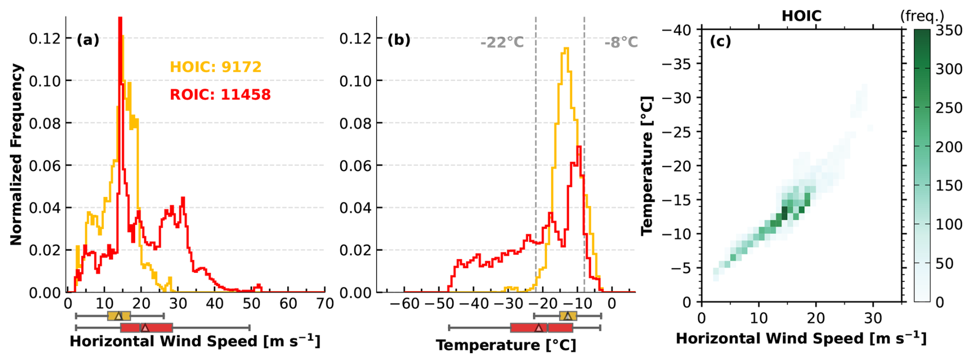
Figure 7 Frequency distributions of environmental variables of different cloud-phase classes on 13 October 2022. (a) The normalized histogram of the horizontal wind speed where HOICs and ROICs exist, with boxplots shown below the x axis. The boxes extend from the lower- to upper-quartile values, with gray lines at the median and triangles at the mean. The whiskers extend from the box to the minimum–maximum values or extend from the box by 1.5 times the interquartile range. The flyers are not shown in the plot. (b) The normalized histogram of temperature where HOICs and ROICs exist, with boxplots shown below the x axis. (c) The density scatterplot of horizontal wind speed and temperature where HOICs exist; the greener the color, the higher the number density of HOIC bins.

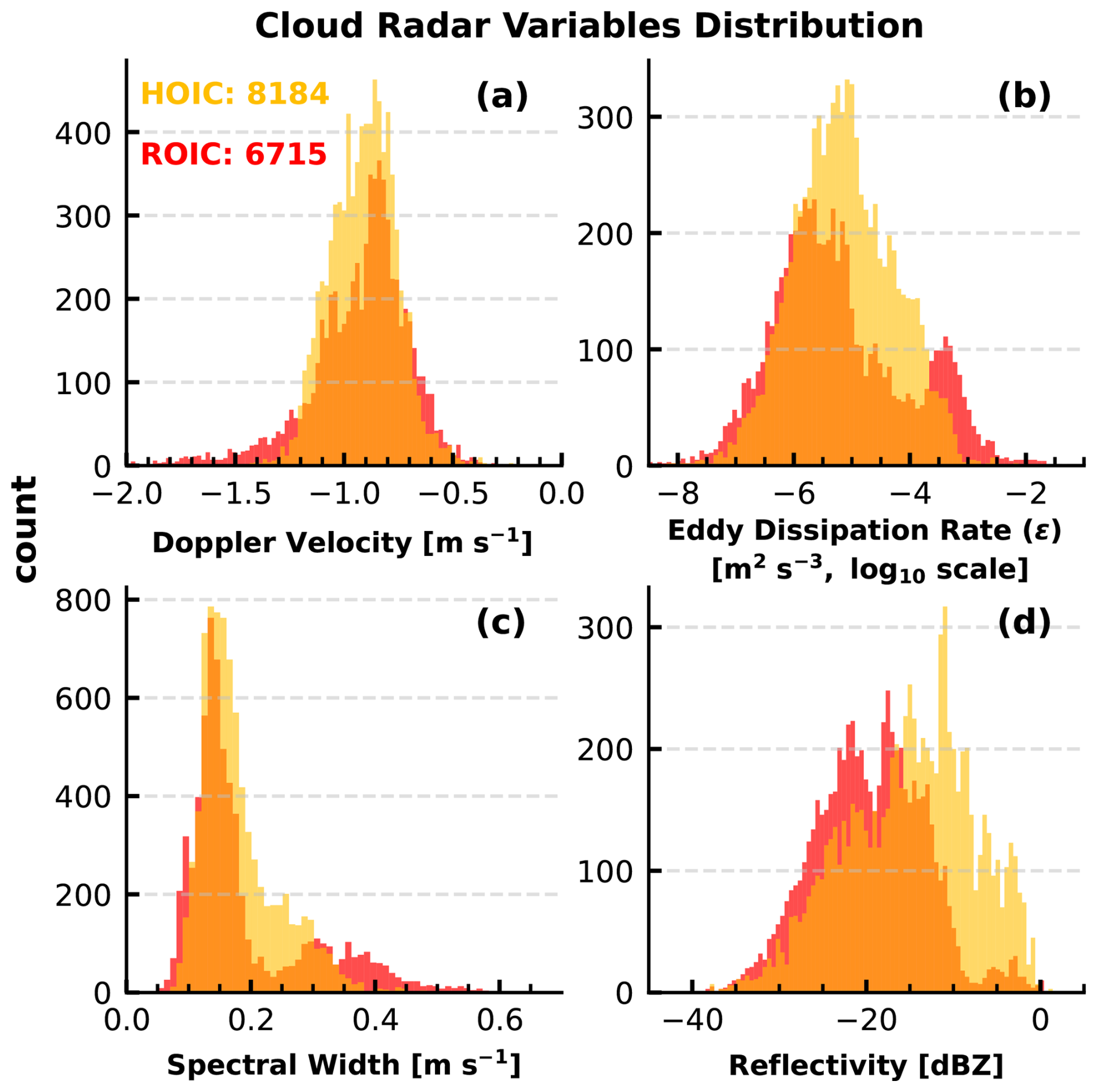
Figure 8 Cloud radar variable distributions of different cloud phases on 13 October 2022. Where HOICs and ROICs exist, (a) the histogram of Doppler velocity, (b) the histogram of retrieved eddy dissipation rate, (c) the histogram of spectral width, and (d) the histogram of reflectivity.

4.3 Cloud radar observations

From cloud radar observations, we can obtain reflectivity, Doppler velocity, and spectral width for HOICs and ROICs, as shown in Fig. 8. The Doppler velocity for HOICs is more narrow and shows a smaller maximum value than that for ROICs, which is consistent with the findings by Westbrook et al. (2010). The median Doppler velocity of HOICs is approximately −0.8 m s⁻¹, and as Westbrook et al. (2010) show from their Doppler lidar observation, the fall speeds for the oriented ice are about −0.3 m s⁻¹. The longer wavelength of the operation of cloud radar, compared to lidar, likely results in the measurement of higher Doppler velocities, as they are more sensitive than lidar to larger particles. Generally, larger particles tend to have higher fall velocities.

Figure 8b shows that the largest eddy dissipation rate ($>{\mathrm{10}}^{-\mathrm{3}}$ m² s⁻³) occurs only with ROICs. Low EDR occurs with both ROICs and HOICs; there are no significant differences between these two orientations. Figure 8c shows that the largest spectral width corresponds to the presence of ROICs. The same behavior is found for the EDR (Fig. 8b). Bimodal structures are found for both EDR and spectral width.

The reflectivity shows larger values for HOICs than ROICs in this case. The peak of the HOICs (around −10 dBZ) is much higher than the peak of the ROICs (around −20 dBZ), indicating that a larger nD⁶ is detected in the bulk of the region where HOICs exist. Contrary to its sensitivity to the presence of columnar ice crystals (Li et al., 2021) or the melting layer (Li and Moisseev, 2020), the cloud radar LDR seems to be rather insensitive to HOICs, as shown in Fig. 4l. This is likely because the LDR of plate-like ice crystals is too small for the current sensitivity of cloud radar to detect.

4.4 Diameter and Reynolds number retrieved for HOICs

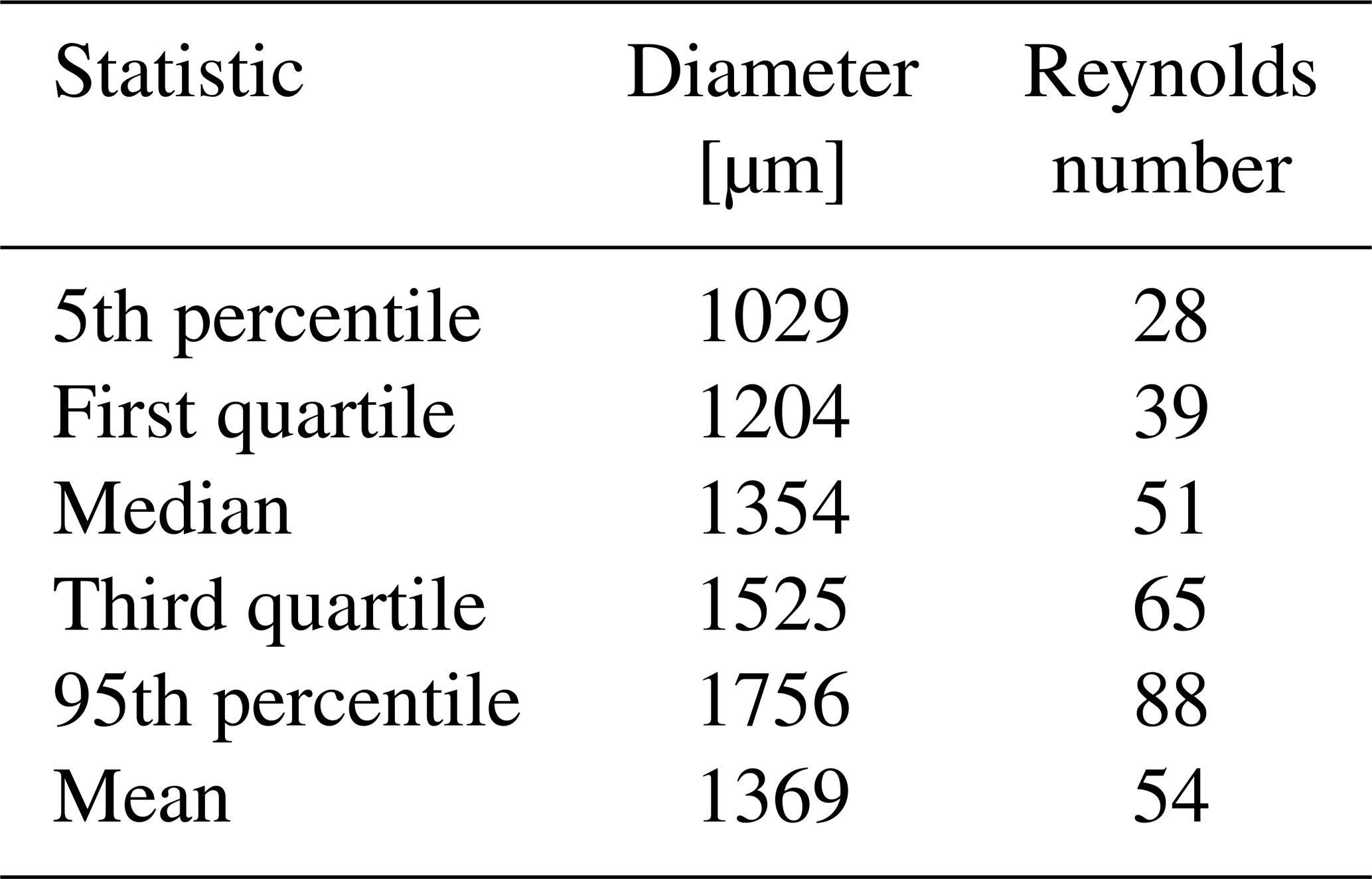
Figure 9 shows the diameter and Reynolds number of HOICs retrieved with an aerodynamic model by assuming that the shape of HOICs can be described by a hexagonal plate. The retrieval methods are described in Appendix D in detail. A summary of the statistical properties of estimated diameters and Reynolds numbers is given in Table 1. The crystal diameters are mostly between 700 and 2000 µm, with a median of 1355 µm and a mean of 1367 µm, which is consistent with the values of 100–3000 µm from Polarization and Directionality of the Earth Reflectances (POLDER) data (Bréon and Dubrulle, 2004, their Fig. 10). Sassen (1980) revealed that a crystal diameter of >100–200 µm is needed for maintaining the horizontal orientation using photographic analyses of light pillar displays. He et al. (2021a) reported estimated diameters of 464–1305 µm for HOICs in 12 cases, with associated Reynolds numbers of 4–58 using a profile-based approach.

Most of the retrieved Reynolds numbers are between 1 and 100 (see Fig. 9d), which coincides with the values of 0.39–80 from the estimation based on spaceborne passive satellite observation (Bréon and Dubrulle, 2004). Bréon and Dubrulle (2004) used a range-bin-based approach to obtain a wider range of Reynolds numbers than the falling-profile-based approach of He et al. (2021a). Kajikawa (1992) measured the lower critical values of the Reynolds number for the unstable falling motion (random orientation) of ice crystals, resulting in 47 to 90.7 based on the different crystal shapes (47 for hexagonal plate).

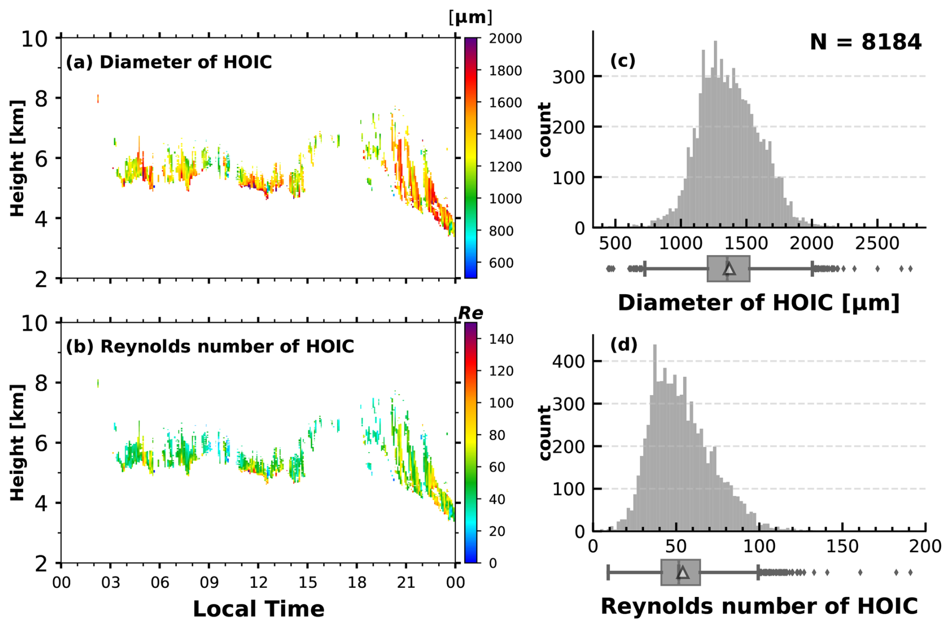
Figure 9 (a) Diameter and (b) Reynolds number of HOICs retrieved on 13 October 2022, time–height contour plots (5 min/15 m resolution). Histograms of HOICs' retrieved diameter (c) and Reynolds number (d), with boxplots below the x axis (the boxes extend from the lower- to upper-quartile values, with gray lines at the median and triangles at the mean; the whiskers extend from the box to the minimum–maximum values or extend from the box by 1.5 times the interquartile range).

Table 1 Statistics of estimated diameters and Reynolds numbers for HOICs on 13 October 2022.

4.5 Relationship between supercooled water cloud and HOICs

At heights above the identified HOIC bins, we can sometimes find some supercooled-water bins. As Westbrook et al. (2010) point out, supercooled water clouds likely play an important role in the formation of HOICs. Since we have a supercooled-water-cloud product (light blue in Figs. 4g and 10), we can also preliminarily investigate the relationship between the occurrence of the supercooled-water-cloud class and HOICs based on the case study.

Especially at times after 16:00, Fig. 4 indicates the supercooled water on top of the identified HOIC regions, which is similar to what has been discussed earlier by, e.g., Westbrook et al. (2010) and He et al. (2021a). The pristine ice crystals which are generated in the supercooled-water layers are probably more liable to maintaining a horizontal orientation. In turn, aging and further processing of ice crystals by means of riming, aggregation, or breakup probably alter the ice crystal structure towards more complex shapes which are associated with a smaller torque and a corresponding lower attitude to maintain the orientation. At times before 16:00 in Fig. 4, the scenario is more complex. For this period, a comparison to the cloud radar observation (Fig. 4k) indicates that the signals of both lidar systems were subject to strong attenuation. For most of the time, the cloud radar detected much higher cloud tops than was identified by the lidars. This was especially the case for those time periods where HOICs were identified. It is thus likely that (1) the HOICs were formed at higher altitudes/lower temperatures and (2) a relationship to the existence of liquid water cannot be directly evaluated because no liquid layers could be identified due to the strong attenuation. Apart from this caveat, the temperatures of the radar-derived cloud tops provide strong hints that liquid water was also involved in the formation of the HOICs observed before 16:00. As noted in Fig. 4k, the top temperatures were generally above −25 °C. It is known from previous studies (De Boer et al., 2011; Westbrook and Illingworth, 2011) that ice forms only via the liquid phase at temperatures above that threshold. It should be noted that the scattering volume of lidars and radar are not exactly the same. Small liquid droplets and optically thin ice clouds are sometimes not detectable from Ka-band radar compared with lidars.

Taking the above-discussed indications for granted, it appears reasonable to evaluate the relationship between the occurrence of liquid water and HOICs in more detail in a quantitative way. While this attempt is promising based on case studies of well-defined scenarios, such as for ice formation in stratiform supercooled liquid clouds, a statistically comprehensive approach that covers the full variety of cloud types is challenging. One reason is that the lidar signal is often already attenuated within the ice virgae below, so no signatures of liquid-dominated ice-forming layers can be observed. Cloud radar techniques, in turn, are frequently not sensitive enough to detect layers of liquid water. The second reason is that the ice-forming supercooled-liquid-water layers might eventually disappear due to cloud dynamical or microphysical processes, while the formed ice particles still exist. A third reason is that vertical wind shear and the microphysical evolution of the ice particles during falling blur the signatures of potential direct relationships between liquid layers and HOIC occurrence.

Here, we introduce the application of the Euclidean distance between supercooled-liquid-water bins and HOICs or ROICs as an approach to quantify the impact of supercooled liquid water on HOIC formation. The relationship which was derived for the observations on 13 October 2022 is shown in Fig. 10. The Euclidean distance is derived by taking the square root of the sum of the squares of the horizontal and vertical distances. The horizontal distance is computed by multiplying the horizontal wind component from ERA5 by the time interval between the bins, while the vertical distance is the height difference between the targeted bins. Moreover, considering the inherent falling characteristics of ice crystals and the general increase in the wind velocity with height, we focus solely on the earlier (leftwards in the time–height cross-section) and higher (upwards in the time–height cross-section) supercooled-water-cloud bins, as they potentially affect the alignment of the ice crystals. From Fig. 10a it can be seen that HOICs in comparison to ROICs are in general closer (brighter in color shade) to regions of supercooled liquid water.

Figure 10b illustrates the quantitative statistical analysis of the Euclidean distance between HOICs and supercooled-water bins. From this figure panel, it is evident that the Euclidean distance for HOICs relative to bins of supercooled liquid water is smaller than that for ROICs, with both a lower median and a lower mean value. This indicates that HOICs are, in general, physically closer to supercooled water clouds. Even considering potential lidar attenuation in this instance, it is still possible to preliminarily conclude that supercooled water droplets may play a significant role in the formation of orientation. It is plausible that pristine ice crystals, generated at cloud top temperatures between −8 and −22 °C, are more likely to induce horizontal orientation with large facets to counteract drag force. Future research should encompass more extensive studies on this subject.

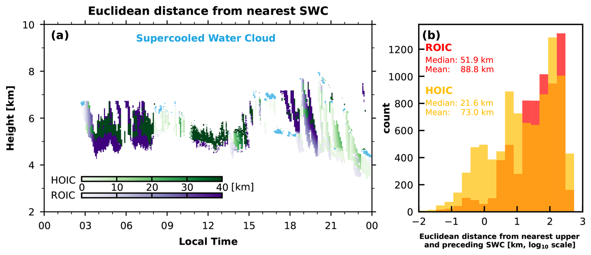
Figure 10 (a) The time–height cross-section of the Euclidean distance between the HOICs, ROICs, and supercooled-water-cloud bins on 13 October 2022. The light-blue range bins represent the supercooled-water-cloud bins. The color indicates the Euclidean distance; the darker the color (dark green and dark purple), the farther the Euclidean distance. Note here that we use a green color bar instead of orange for HOICs and a purple color bar instead of red for ROICs to better discriminate HOICs and ROICs with different shades of the same color. (b) The histogram of the Euclidean distance between the HOICs, ROICs, and supercooled-water-cloud bins on 13 October 2022 in log₁₀ scale with the median and mean values noted in the upper-left corner.

5 Summary and conclusions

In this study, we developed a novel range-resolved detection method for horizontally oriented ice crystals (HOICs) using a combination of zenith-pointing and 15° off-zenith-pointing polarization lidars, in Beijing, China. In synergy with collocated observations from cloud radar, radiosonde data, and the ERA5 dataset, our approach provides unprecedented detail regarding HOIC detection and the characterization of HOICs. This enhancement facilitates improvements in both the spatial and the temporal resolution of these observations, thereby enabling a comprehensive investigation into the phenomenological aspects of HOIC events. One of the key findings of this research concerns the enhanced turbulence eddy dissipation rates (EDR) observed near the cloud base, which corresponds to the “switch-off” phenomenon of horizontal orientation in ice crystals. We attribute this phenomenon to the latent heat released from ice crystal sublimation. This discovery represents a significant advancement over previous studies, providing new insights into the role of turbulence in disrupting the horizontal alignment of ice crystals.

Our case study showed that HOICs form in relatively warm temperatures (−8 to −22 °C) where plate-like ice crystals exist and in the presence of rather light wind speeds (0–20 m s⁻¹). Cloud radar indicates that mean Doppler velocity is similar for HOICs and ROICs (randomly oriented ice crystals) but more concentrated for HOICs. The highest EDR and spectral width are exclusive to ROICs, while HOICs generally have larger reflectivity. Moreover, the estimated diameter using Doppler cloud radar and the aerodynamic model (ranging from approximately 1029 to 1756 µm for 5th and 95th percentiles) and Reynolds numbers (28 to 88 for 5th and 95th percentiles) provide a clearer understanding of HOICs' microphysical properties. Moreover, our observations suggest a strong relationship between supercooled water clouds and HOIC formation, with a closer Euclidean distance between supercooled-water-cloud bins for HOICs compared to ROICs. The HOICs persisted for nearly the whole day in this case, indicating that they could significantly impact the radiation balance. These findings could help improve the parameterization schemes in climate models, especially in mid-latitude regions like Beijing.

In this paper, we only show one typical case to demonstrate the HOIC identification method. More case studies could be shown in following work to show different conditions for HOICs (different cloud top temperatures). The observation method and detection algorithm developed in this research provide new tools for long-term HOIC observation due to the precise range bin identification of HOICs and continuous observation; future work of diurnal and seasonal characteristics will be established through the yearlong dataset. Since this dataset enables the joint classification of both supercooled-water-cloud bins and HOICs, it provides a unique dataset to investigate the relationship between supercooled water and HOICs, which could shed light on the generation mechanism of HOICs, as previously revealed by Westbrook et al. (2010), and the Euclidean-distance approach presented within our study. We see a high potential in using the Euclidean-distance approach, even though an improved quantification will require an enhanced characterization of the presence of liquid water beyond lidar attenuation (e.g., Schimmel et al., 2022) and an improved consideration of the ice crystal evolution during sedimentation (Vogl et al., 2024). Beyond the relationship between supercooled water and HOICs, recent studies suggest that HOICs are often correlated to precipitating clouds and that their ice nucleation processes have a connection with precipitation formation (Ross et al., 2017; Kikuchi and Suzuki, 2019). In addition, the orientation of ice crystals is always a mixture in a bulk volume, and the horizontal orientation is approximately quasi-horizontally oriented, with some flutter or wobbling angles. The fraction of HOICs inside a range bin and the flutter angle could be retrieved with the help of HOIC model data (Borovoi et al., 2018; Saito and Yang, 2019). Further studies are required to help derive the ratio of $\mathrm{HOIC}/\mathrm{ROIC}$. What's more, in this study, we only use two elastic lidars; long-term Raman lidar and HSRL (high-spectral-resolution lidar) observation could be employed to accurately determine the lidar ratio and particle depolarization ratio to provide more information about HOICs in the future.

Like all lidar-based research, lidar attenuation for opaque clouds (i.e., optical depths roughly above 3) is a main defect of this method, so some upmost cloud range bins are missed. With cloud radar, we can infer the cloud top beyond lidar attenuation to a certain extent. Future ice crystal orientation detection work based on radar should be carried out to make up for this defect (Hajipour et al., 2024). The assumption of pure hexagonal plates in the diameter and Reynolds number retrieval is the simplest: highly symmetrical crystal. In practice, many other planar crystals exist. Using Doppler velocity to estimate the ice crystal diameter is a rough estimation because the superposition of air movement is ignored. Future retrieval could consider deriving the ice crystal size utilizing the ratio of radar reflectivity and the lidar extinction (Bühl et al., 2019; Ansmann et al., 2024). So some uncertainty could exist in the process of estimating diameters and Reynolds numbers. We only consider the middle part of the retrieved data, without the extreme values. In conclusion, we find the collection of retrieval techniques and approaches for HOIC classification and characterization that was presented in this study to comprise a valuable toolset for statistical evaluations that cover longer time periods. This possibility is granted by means of the 1-year dataset from Beijing that was introduced only briefly here. In a follow-up study, a statistical evaluation of the relationship between HOICs and other cloud microphysical and environmental parameters will be presented.

Appendix A: AVORS lidar optomechanical setup

Figure A1 is the optomechanical setup of the AVORS lidar, an image courtesy of AVORS Technology. Note two photomultiplier tubes (PMTs, model Hamamatsu H10682-210) are used in the system.

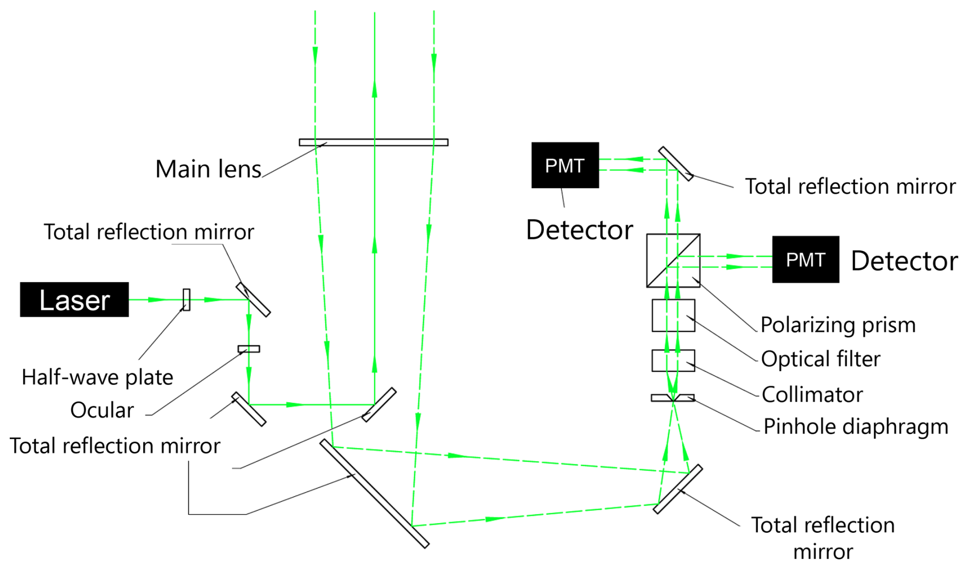
Figure A1 Schematic of the AVORS lidar optomechanical setup. Image courtesy of AVORS Technology.

Table A1 Specifications of the Portable Particle Lidar by AVORS Technology.

Appendix B: Lidar calibration

B1 Lidar system constant calibration

This step converts the lidar's original photon count into attenuated backscatter, enabling the comparison of backscatter signals between zenith-pointing and off-zenith-pointing lidars. First, the MPL and AVORS lidar both use a photon count system: the photon count rate times dead time correction minus the afterpulse value for MPL (there is no need to subtract the afterpulse value for the AVORS lidar after the manufacturer's test) minus the background times the square of the range and divided by the overlap function times laser energy. The above steps are summarized as Eqs. (B1) and (B2):

$$\begin{array}{}\text{(B1)}& \begin{array}{rl}& {\text{NRB}}_{\text{MPL}}=\\ & {\displaystyle \frac{\begin{array}{c}\left[(\mathrm{photon}\mathrm{count}\mathrm{rate}\times \mathrm{dead}\mathrm{time}\mathrm{correction})-\right.\\ \left.\mathrm{afterpulse}-\mathrm{background}\right]\times {\mathrm{range}}^{\mathrm{2}}\end{array}}{\mathrm{overlap}\times \mathrm{laser}\mathrm{energy}}}\end{array},\end{array}$$

$$\begin{array}{}\text{(B2)}& \begin{array}{rl}& {\text{NRB}}_{\text{AVORS}}=\\ & {\displaystyle \frac{\begin{array}{c}\left[(\mathrm{photon}\mathrm{count}\mathrm{rate}\times \mathrm{dead}\mathrm{time}\mathrm{correction})-\right.\\ \left.\mathrm{background}\right]\times {\mathrm{range}}^{\mathrm{2}}\end{array}}{\mathrm{overlap}\times \mathrm{laser}\mathrm{energy}}}\end{array}.\end{array}$$

In this way, we get the normalized relative backscatter (NRB). Then we employ PollyNet's calibration method (Baars et al., 2016; Yin et al., 2020) to two lidars' NRB profiles; namely we first find the Rayleigh fit, i.e., the aerosol-free region. Then we assume a fixed lidar ratio of 50 sr, using the Klett–Fernald method to retrieve the extinction profile (Fernald, 1984). After that, we integrate the extinction profiles to get the height-resolved aerosol optical depth (AOD) and the lidar calibration constant; then we employ a smooth method to the lidar calibration constant profile to determine the final lidar calibration constant. After that, the attenuated backscatter can be derived by NRB divided by the lidar calibration constant.

B2 Lidar depolarization calibration

Lidar depolarization is the key feature that distinguishes the HOICs. HOICs show a much lower depolarization ratio than ROICs for zenith-pointing lidar (He et al., 2021a). Before the identification of HOICs, we must confirm the reliability of our lidars' depolarization ratio. Since the MPL and AVORS lidar are both compact, small-sized lidars, the standard Δ90 method (Freudenthaler, 2016) is not applicable. We use the well-calibrated Raman lidar to get the depolarization ratio and match the same time's MPL and AVORS lidar depolarization ratio.

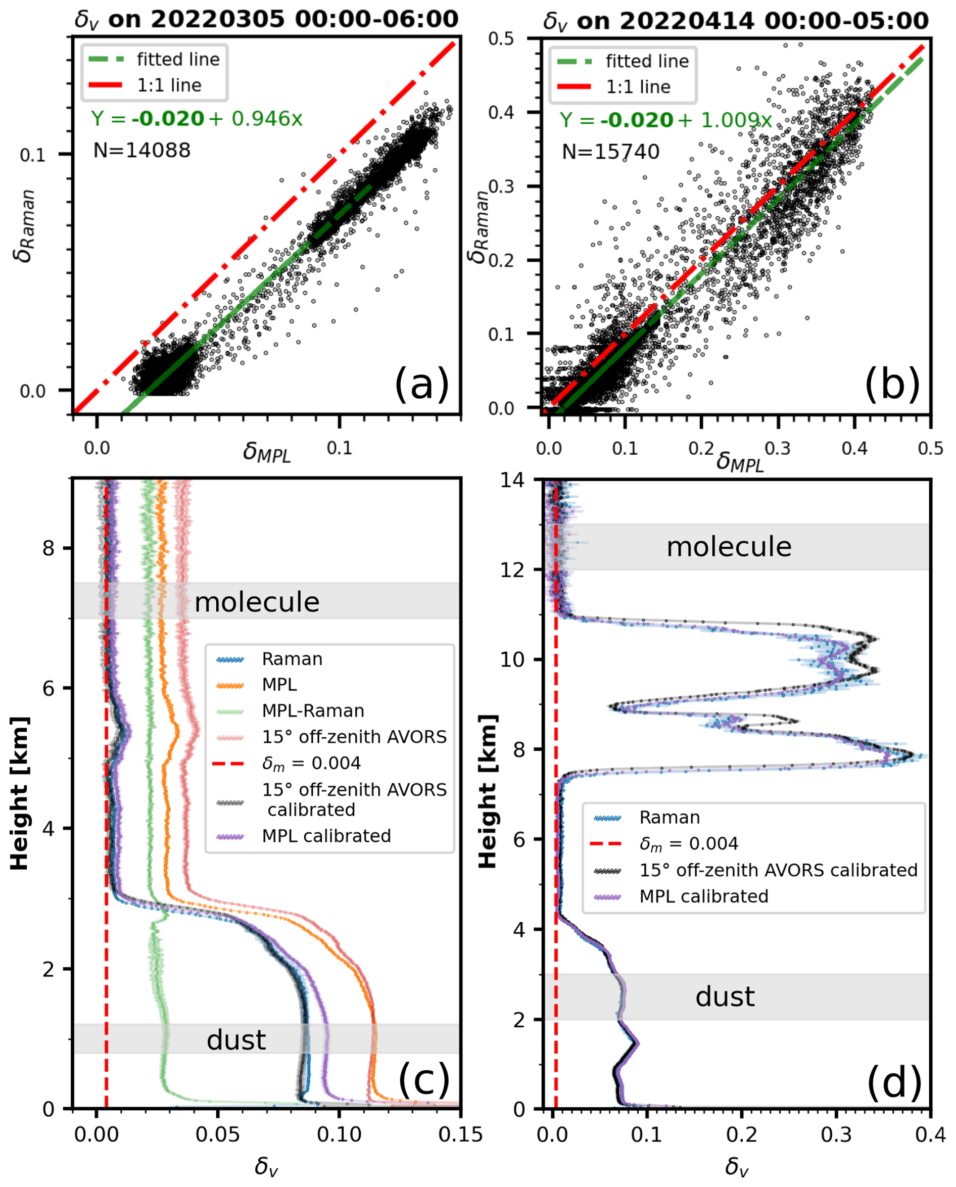
Figure B1 Scatterplot of the well-calibrated Raman lidar and MPL uncalibrated depolarization ratio on (a) 5 March 2022, 00:00–06:00 LT, and (b) 14 April 2022, 00:00–05:00 LT; (c) averaged depolarization profiles on 5 March 2022, 0:00–06:00; (d) averaged depolarization profiles on 14 April 2022, 00:00–05:00; the horizontal gray-shaded areas indicate the reference ranges used for dust and molecular layers. The shaded regions around the lines represent the uncertainties associated with depolarization ratio calculation and calibration.

Due to the MPL having only one detector for two polarization channels (Flynna et al., 2007), there is no gain ratio effect here (or the gain ratio $K^{*}=\mathrm{1}$ in the case of Papetta et al., 2024; see Eq. B3); we use the Córdoba-Jabonero et al. (2021) method to calibrate the MPL's depolarization, namely assuming a constant deviation compared with the reference Raman lidar. Figure B1a and b are the scatterplots between the MPL depolarization ratios and reference Raman lidar depolarization ratios on 5 March 2022 from 00:00 to 06:00 and 14 April 2022 from 00:00 to 05:00, respectively, showing a constant intercept of $-\mathrm{0.020}\pm \mathrm{0.001}$. Additional cases (not shown here) from 00:00 to 01:00 on 26 February 2022 and from 00:00 to 05:00 on 7 May 2022 further validate the consistency of the −0.02 offset. Then we simply use ${\mathit{\delta }}_{\text{MPLcalibrated}}={\mathit{\delta }}_{\text{MPL}}-\mathrm{0.02}$ to calibrate the MPL depolarization. Figure B1c and d show the calibrated MPL depolarization ratio profiles (purple) and the observed uncalibrated ones (orange), indicating good agreement of the depolarization ratio between the calibrated MPL and the reference Raman lidar. Note, as is shown in Fig. B1c, for the calibrated MPL depolarization ratio profile, there is a slight residual difference from the Raman lidar (≈0.01) below 2.5 km, but it is still acceptable. From our observation, the region below 2 km, where this difference is most pronounced, is generally unimportant for identifying HOICs (in the 13 October 2022 case, HOICs are above 4 km). Therefore, the imperfect performance of the calibrated depolarization ratio in this layer has minimal impact on HOIC detection.

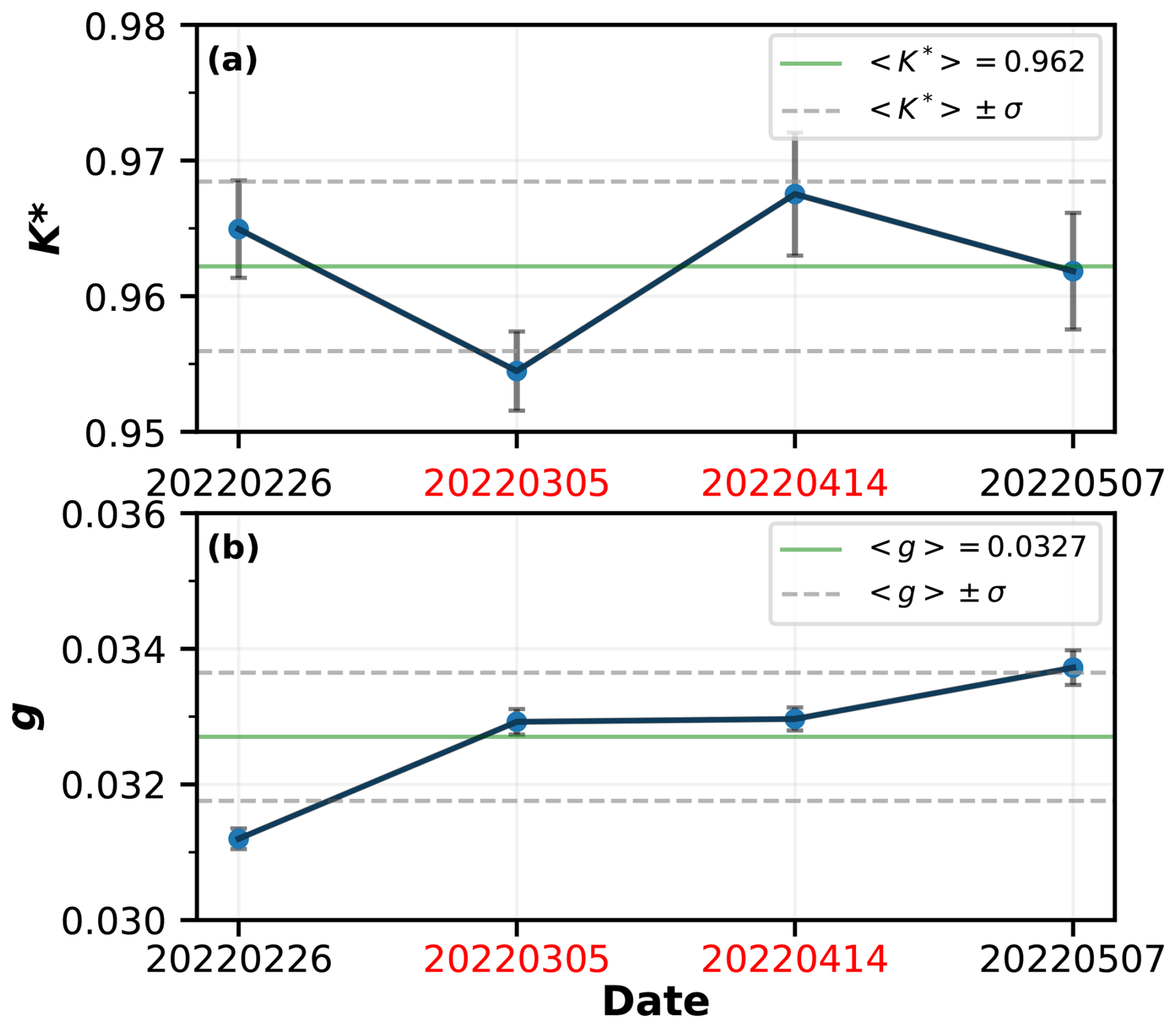
Figure B2 Temporal evolution of polarization parameters derived using the two-parameter approach. Error bars indicate the variability in the derived parameters within the selected molecular scattering and dust reference layers. The average polarization parameter value and its standard deviation in the whole period are shown by solid green lines and dashed gray lines, respectively. The timestamps of the cases shown in Fig. B1 are highlighted in red.

For the AVORS lidar, since it has two detectors for each polarization channel (similar to the Cimel CE376 lidar system used in the case of Papetta et al., 2024; see Fig. A1), we use the newly proposed two-parameter method of Papetta et al. (2024, their Eq. 10) to calibrate the depolarization of the lidars. The two parameters are K^*, the gain ratio between the two channels, and g, the cross-talk from the co-polar signal to the cross-polar signal.

Using δ^* to denote the uncalibrated AVORS lidar depolarization ratio or the observed depolarization ratio, the calibrated AVORS lidar depolarization ratio (δ) can be expressed using K^* and g:

$$\begin{array}{}\text{(B3)}& \mathit{\delta }={\displaystyle \frac{{\mathit{\delta }}^{*}}{K^{*}}}-g.\end{array}$$

Then we select one dust layer and one aerosol-free region as reference; we use ${\mathit{\delta }}_{\mathrm{ref}}^{\mathrm{d}}$ from the reference Raman lidar observation and theoretical molecular depolarization δ_m of 0.004 (Behrendt and Nakamura, 2002), and we select the observed lidar depolarization ratio of the dust layer (${\mathit{\delta }}_{\mathrm{d}}^{*}$) and the molecular layer (${\mathit{\delta }}_{\mathrm{m}}^{*}$).

$$\begin{array}{}\text{(B4)}& {\mathit{\delta }}_{\mathrm{ref}}^{\mathrm{d}}={\displaystyle \frac{{\mathit{\delta }}_{\mathrm{d}}^{*}}{K^{*}}}-g\end{array}$$

$$\begin{array}{}\text{(B5)}& {\mathit{\delta }}_{\mathrm{m}}={\displaystyle \frac{{\mathit{\delta }}_{\mathrm{m}}^{*}}{K^{*}}}-g\end{array}$$

With two unknowns and two equations, K^* and g can be solved using

$$\begin{array}{}\text{(B6)}& K^{*}={\displaystyle \frac{{\mathit{\delta }}_{\mathrm{d}}^{*}-{\mathit{\delta }}_{\mathrm{m}}^{*}}{{\mathit{\delta }}_{\mathrm{ref}}^{\mathrm{d}}-{\mathit{\delta }}_{\mathrm{m}}}},\end{array}$$

$$\begin{array}{}\text{(B7)}& g={\displaystyle \frac{{\mathit{\delta }}_{\mathrm{m}}^{*}{\mathit{\delta }}_{\mathrm{ref}}^{\mathrm{d}}-{\mathit{\delta }}_{\mathrm{d}}^{*}{\mathit{\delta }}_{\mathrm{m}}}{{\mathit{\delta }}_{\mathrm{d}}^{*}-{\mathit{\delta }}_{\mathrm{m}}^{*}}}.\end{array}$$

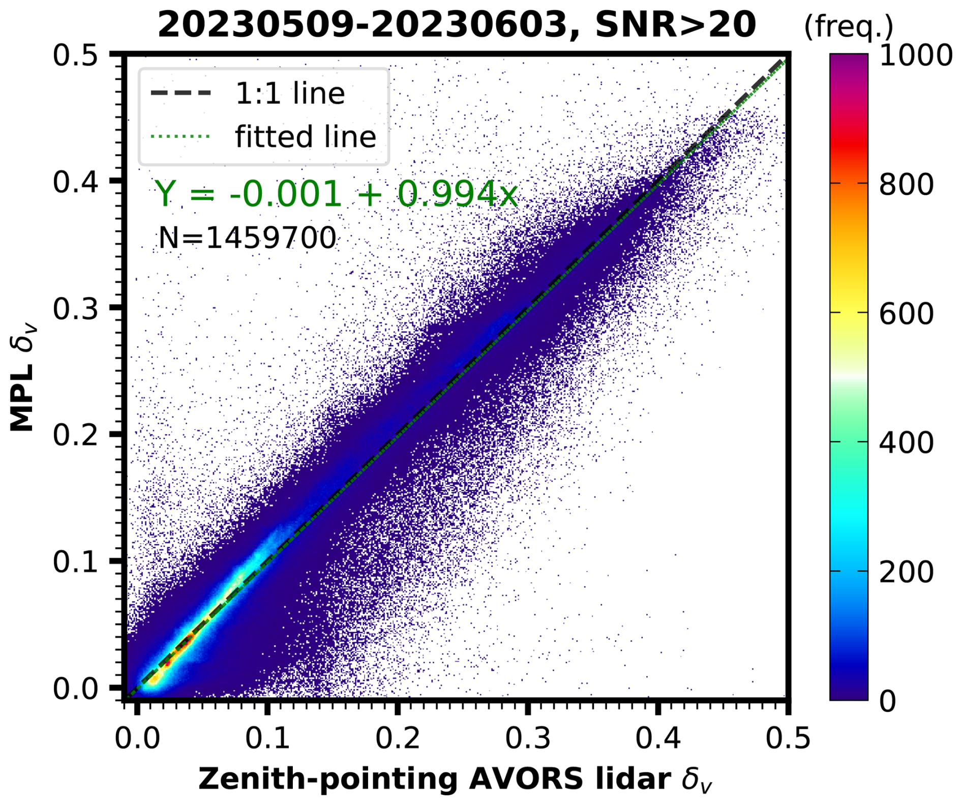
Figure B3 The density scatterplot between the zenith-pointing AVORS lidar and the MPL calibrated depolarization ratio from 9 May to 3 June 2023, when the two lidars were both zenith-pointing. Points including clouds, aerosols, and molecules with signal-to-noise ratios greater than 20 are used to plot the figure.

What's more, Fig. B1c shows the case (5 March 2022, 00:00–06:00) used for AVORS lidar depolarization calibration. Similar to the case of Papetta et al. (2024), we select the molecule region around 7–7.5 km (Eq. B5) and dust region around 1 km (Eq. B4) as reference; both regions are denoted with a gray frame in Fig. B1c. After that we can get $K^{*}=\mathrm{0.954}$ and g=0.0329 from Eqs. (B6) and (B7). Three additional cases – 00:00–01:00 on 26 February 2022, 00:00–05:00 on 14 April 2022, and 00:00–05:00 on 7 May 2022 – were selected using a consistent method involving molecule and dust regions to derive robust K^* and g values. The resulting K^* and g values are presented in Fig. B2 with statistics. Ultimately, we obtained $K^{*}=\mathrm{0.962}\pm \mathrm{0.006}$ and $g=\mathrm{0.0327}\pm \mathrm{0.0009}$. The calibrated-depolarization-ratio profile was calculated from Eq. (B3) using the robust K^* and g. Figure B1c shows the calibrated AVORS lidar depolarization (black) and the observed one (pink). We can find that after calibration, the AVORS lidar depolarization ratio is very close to the reference Raman lidar (see Fig. B1c, black line and blue line).

Figure B1d shows the calibrated MPL and AVORS lidar and the Raman lidar depolarization ratio profiles on 14 April 2022 from 00:00 to 05:00 (another case). For the molecule region (above 11 km) and dust region (below 4 km), the three lidars' depolarization ratio profiles match perfectly, indicating that the calibration method used here for two lidars shows good performance. For the cirrus region between 7.5 and 11 km, however, there is a slight difference between the three lidars' depolarization ratios, which could be explained by the three lidars having different fields of view (Raman, 2.3 mrad; MPL, 0.1 mrad; AVORS, 0.2 mrad), multiple-scattering effects with the cloud could contribute some uncertainty. Besides, since the AVORS lidar was off-zenith-pointing (Raman lidar and MPL are both zenith-pointing), some horizontal heterogeneity of the cirrus might exist. Nevertheless, the slight difference does not prevent our algorithm (Fig. 2) from distinguishing HOICs. Sensitivity tests were performed to evaluate the stability of the 0.6 threshold (ratio of zenith to off-zenith depolarization) used in the classification flowchart (Fig. 2). Assuming typical depolarization uncertainties (5 %–10 %, percent error) as shown in Fig. B1, the analysis based on long-term statistics of ice-containing clouds indicates that the percentage of falsely identified HOICs and ROICs is below 2 %–5 %, which corroborates the tolerance of the classification scheme to uncertainties in the depolarization. Note that the Raman lidar depolarization matches the theoretical molecular depolarization value of 0.004 very well (Fig. B1c and d above 7 and 11 km, respectively), showing excellent depolarization performance as a reference lidar.

There is a period (from 9 May to 3 June 2023) when both MPL and AVORS lidar were zenith-pointing; we can utilize this period to validate our depolarization calibration result. Figure B3 shows the density scatterplot of the MPL and AVORS lidar calibrated depolarization ratio of the cloud, aerosol, and molecule range bins observed during both lidars' zenith-pointing period. The least-squares fitting line (dashed green line) nearly overlaps with the 1:1 line (dashed black line), indicating good agreement of the two lidars' depolarization after calibration. According to the methods described above, we use the calibrated depolarization of MPL and the AVORS lidar for the categorization algorithm and other analysis in this study.

Appendix C: Description of RH calculation

The vapor pressure E can be calculated from the following equation:

$$\begin{array}{}\text{(C1)}& E={\displaystyle \frac{rP}{\mathrm{0.622}+r}},\end{array}$$

where r is the water vapor mixing ratio. Here we use the specific humidity (q) from the ERA5 data ($r=\frac{q}{\mathrm{1}-q}$; since q≪1, r≈q).

The saturated water vapor pressure with respect to liquid water E_w and ice E_i can be calculated from the following empirical formulas (Murray, 1967; Bolton, 1980):

$$\begin{array}{}\text{(C2)}& E_{\text{w}}=\mathrm{6.112}\text{exp}\left[{\displaystyle \frac{\mathrm{17.67}(T-\mathrm{273.16})}{T-\mathrm{29.65}}}\right],\end{array}$$

$$\begin{array}{}\text{(C3)}& E_{\text{i}}=\mathrm{6.1078}\text{exp}\left[{\displaystyle \frac{\mathrm{21.87}(T-\mathrm{273.16})}{T-\mathrm{7.66}}}\right],\end{array}$$

where T is the temperature provided by radiosonde or ERA5. Then, relative humidity over water (RH_w) and ice (RH_i) can be calculated by

$$\begin{array}{}\text{(C4)}& {\mathrm{RH}}_{\mathrm{w}}={\displaystyle \frac{E}{E_{\text{w}}}},\end{array}$$

$$\begin{array}{}\text{(C5)}& {\mathrm{RH}}_{\mathrm{i}}={\displaystyle \frac{E}{E_{\text{i}}}}={\displaystyle \frac{{\mathrm{RH}}_{\mathrm{w}}{E}_{\text{w}}}{E_{\text{i}}}}.\end{array}$$

For radiosonde, RH_w is provided; we use Eqs. (C2), (C3), and (C5) to get the RH_i profile. For ERA5 RH_i data, however, relative humidity is a piecewise function of saturation over water and ice (>0 °C over water, $<-\mathrm{23}$ °C over ice, between −23 and 0 °C interpolating the value over ice and water). We use the specific humidity to calculate RH_i and RH_w separately (Eqs. C1 to C5).

Appendix D: Reynolds number and diameter calculation for falling ice crystals

For further discussion, the diameter and Reynolds number of horizontally oriented ice crystals can be estimated from the terminal falling velocity measured by Doppler cloud radar (He et al., 2021a). Here we use the approach proposed by Heymsfield and Westbrook (2010). First, as the columns have a negligible impact on specular reflection compared to the plates (Zhou et al., 2012a), which present significantly larger surfaces to the incident lidar beam, we assume the HOIC shape is a hexagonal plate and the thickness h is 0.04D, where D is the diameter of the ice crystal (Beard, 1980). The mass of a single ice crystal is then $m=\frac{\mathrm{3}\sqrt{\mathrm{3}}}{\mathrm{8}}{D}^{\mathrm{2}}\times h\times {\mathit{\rho }}_{\mathrm{ice}}$. The area ratio of ice crystal A_r is defined as $A_{\mathrm{r}}=A/\left[\right(\mathit{\pi }/\mathrm{4}\left)D^{\mathrm{2}}\right]$. For horizontally oriented hexagonal plate ice crystals, A_r=0.827.

The corresponding modified Davies number is defined as

$$\begin{array}{}\text{(D1)}& X={\displaystyle \frac{{\mathit{\rho }}_{\mathrm{air}}}{{\mathit{\eta }}^{\mathrm{2}}}}{\displaystyle \frac{\mathrm{8}\mathrm{mg}}{\mathit{\pi }{A}_{\mathrm{r}}^{\mathrm{1}-k}}},\end{array}$$

where the optimum value of k is 0.5. The density of air ρ_air is the function of pressure (P) and temperature (T) and can be calculated by

$$\begin{array}{}\text{(D2)}& {\mathit{\rho }}_{\mathrm{air}}=\mathrm{1.293}\times {\displaystyle \frac{P}{P_{\mathrm{0}}}}\times {\displaystyle \frac{\mathrm{273.15}}{T}},\end{array}$$

where P₀ set to 1013.25 hPa is the standard atmospheric pressure and P and T are interpolated from ERA5 data.

Air dynamic viscosity η is defined as

$$\begin{array}{}\text{(D3)}& \mathit{\eta }={\mathit{\eta }}_{\mathrm{0}}\times {\left({\displaystyle \frac{T}{\mathrm{288.15}}}\right)}^{\mathrm{1.5}}\times {\displaystyle \frac{\mathrm{288.15}+B}{T+B}},\end{array}$$

where η₀ is the air dynamic viscosity at 15 °C, ${\mathit{\eta }}_{\mathrm{0}}=\mathrm{1.7894}\times {\mathrm{10}}^{-\mathrm{5}}$ Pa s (T=15 °C), and B is a gas-type-related constant, B=110.4 K.

The Reynolds number Re can be expressed as a function of the Davies number:

$$\begin{array}{}\text{(D4)}& Re={\displaystyle \frac{{\mathit{\delta }}_{\mathrm{0}}^{\mathrm{2}}}{\mathrm{4}}}\left[{\left(\mathrm{1}+{\displaystyle \frac{\mathrm{4}\sqrt{X}}{{\mathit{\delta }}_{\mathrm{0}}^{\mathrm{2}}\sqrt{C_{\mathrm{0}}}}}\right)}^{\mathrm{1}/\mathrm{2}}-\mathrm{1}\right],\end{array}$$

where the inviscid coefficient C₀=0.35 and the dimensionless coefficient δ₀=8.0. Finally, the crystal diameter D can be calculated through the following equation:

$$\begin{array}{}\text{(D5)}& D={\displaystyle \frac{\mathit{\eta }Re}{{\mathit{\rho }}_{\mathrm{air}}{v}_t}},\end{array}$$

where v_t is estimated by the cloud radar Doppler velocity.

Finally, from Eqs. (D1), (D4), and (D5), we can retrieve the diameter of the horizontally oriented ice crystal and the corresponding Reynolds number. After conducting careful sensitivity tests, we found that the assumed fixed aspect ratio ($h/D$) of 0.04 yields a retrieved diameter and Reynolds number similar to those obtained using empirical dynamic aspect ratio relationships reported in the literature (Bréon and Dubrulle, 2004; Saito and Yang, 2019). It is important to note that crystal diameter and Reynolds number are highly sensitive to the shape of ice crystals (Westbrook et al., 2010, their Table III). The assumed HOIC shape of hexagonal plates is the most simplified and widely used model (Bréon and Dubrulle, 2004; Zhou et al., 2012b; He et al., 2021a). Additionally, assuming that Doppler velocity represents the terminal velocity of a particle in still air introduces some uncertainty. However, in general, long-term Doppler velocity measurements can partially mitigate the effect of rapidly changing vertical airflow and provide an approximate still-air velocity for falling ice crystals. To reduce the potential uncertainty caused by extreme vertical airflow, we focus only on the intermediate range of the retrieved diameters and Reynolds numbers, excluding extreme values (e.g., data points beyond the 5th and 95th percentiles). In summary, this method serves as an estimation to compare the case with previous studies (Westbrook et al., 2010; He et al., 2021a).

Appendix E: Calculation of eddy dissipation rates

The turbulence eddy dissipation rate (or turbulent kinetic energy dissipation rate, EDR, ϵ) is a measure of the rate at which turbulent kinetic energy is converted into thermal energy due to viscous dissipation in a fluid. It quantifies how energy from larger turbulent eddies is transferred to smaller eddies and ultimately dissipated as heat, indicating the intensity of turbulence. The turbulence eddy dissipation rate was computed to reflect the turbulence using quantities including the standard deviation of Doppler velocity and horizontal wind speed in this study (Bouniol et al., 2003; O’Connor et al., 2010).

The standard deviation of the average wind serves as a measure of the kinetic energy present at turbulent scales that are typically larger than the size of the sampled volume. ϵ can be inferred from the variability in the vertical velocity over the 300 s sample time; ${\mathit{\sigma }}_{\stackrel{\mathrm{‾}}{v}}$ in Eq. (E1) is the standard deviation of Doppler velocity within 300 s for 13 s unit time. By integrating the Kolmogorov (1941) turbulent energy spectrum formula within the inertial subrange, we can get

$$\begin{array}{}\text{(E1)}& \mathit{ϵ}={\left({\displaystyle \frac{\mathrm{2}}{\mathrm{3}a}}\right)}^{\mathrm{3}/\mathrm{2}}{\displaystyle \frac{{\mathit{\sigma }}_{\stackrel{\mathrm{‾}}{v}}^{\mathrm{3}}}{{\left(k^{-\mathrm{2}/\mathrm{3}}-{k_{\mathrm{1}}}^{-\mathrm{2}/\mathrm{3}}\right)}^{\mathrm{3}/\mathrm{2}}}},\end{array}$$

where a=0.55 is the one-dimensional Kolmogorov constant (Borque et al., 2016). The wave number related to the large eddies traveling through the sampling volume during the sampling time is

$$\begin{array}{}\text{(E2)}& k={\displaystyle \frac{\mathrm{2}\mathit{\pi }}{x_{\mathrm{b}}+T_{\mathrm{s}}\left|V_{\mathrm{h}}\right|}},\end{array}$$

where the width of the radar beam at height z is $x_{\mathrm{b}}=\mathrm{2}z\sin (\mathit{\theta }/\mathrm{2})$ with θ=0.35° for this cloud radar. $\left|V_{\mathrm{h}}\right|$ is the modulus of the horizontal wind, interpolated from ERA5 data. T_s is the sampling time, 300 s in this case. And the wave number corresponding to the length scale describing the scattering volume dimension for the dwell time for a single sample is given by

$$\begin{array}{}\text{(E3)}& k_{\mathrm{1}}={\displaystyle \frac{\mathrm{2}\mathit{\pi }}{x_{\mathrm{b}}+t\left|V_{\mathrm{h}}\right|}},\end{array}$$

where dwell time t=13 s for this cloud radar's case. In this way, the turbulence eddy dissipation rate was estimated from Eqs. (E1), (E2), and (E3). Note that Bouniol et al. (2003) use the time period of 30 s for ${\mathit{\sigma }}_{\stackrel{\mathrm{‾}}{v}}$ and show that the estimated EDRs are not sensitive to the number of points used. A recent study (Nijhuis et al., 2019) points out that 10 min is still within the inertial subrange, so we use the 300 s (5 min) time interval to calculate standard deviation considering consistency with other quantities' time resolution in this study.

Appendix F: List of abbreviations and symbols

CALIPSO	Cloud-Aerosol Lidar and Infrared Pathfinder
	Satellite Observations
CALIOP	Cloud-Aerosol Lidar with Orthogonal
	Polarization
DSCOVR	Deep Space Climate Observatory
EDR	eddy dissipation rate
ECMWF	European Centre for Medium-Range Weather
	Forecasts
EPIC	Earth Polychromatic Imaging Camera
ERA5	ECMWF Reanalysis v5
EarthCARE	Earth Cloud, Aerosol and Radiation Explorer
HOIC	horizontally oriented ice crystal
LDR	linear depolarization ratio
MMCR	millimeter-wave cloud radar
MPL	Micro Pulse Lidar
MPC	mixed-phased cloud
NRB	normalized relative backscatter
PKU	Peking University
PMT	photomultiplier tube
POLDER	Polarization and Directionality of the Earth
	Reflectance
RH	relative humidity
ROIC	randomly oriented ice crystal
SNR	signal-to-noise ratio
SWC	supercooled liquid water cloud
TKE	turbulent kinetic energy
β′	attenuated backscatter
${\mathit{\beta }}_{\text{zenith}}^{\prime }$	attenuated backscatter of zenith-pointing lidar
${\mathit{\beta }}_{\text{off-zenith}}^{\prime }$	attenuated backscatter of off-zenith-pointing
	lidar
δv(δ)	volume depolarization ratio
δzenith	volume depolarization ratio of zenith-pointing
	lidar
δoff-zenith	volume depolarization ratio of
	off-zenith-pointing lidar