the Creative Commons Attribution 4.0 License.
the Creative Commons Attribution 4.0 License.
 | 11 Aug 2025
Improved simulation of thunderstorm characteristics and polarimetric signatures with LIMA two-moment microphysics in AROME
Clotilde Augros
Benoit Vié
François Bouttier
Tony Le Bastard
Thunderstorm forecasting remains challenging despite advances in numerical weather prediction (NWP) systems. The microphysics scheme that represents clouds in the model partly contributes to the introduction of uncertainties in the simulations. To better understand the discrepancies, synthetic radar data simulated by a radar forward operator (applied to model outputs) are usually compared to dual-polarization radar observations, as they provide insight into the microphysical structure of clouds. However, the modeling of polarimetric values and radar signatures such as the ZDR column (ZDRC) remains a complex issue, despite the diversity of microphysics schemes and forward operators, especially above the freezing level where values that are too low are often found.
The aim of this work is to assess the ability of the AROME NWP convective model, when coupled with two distinct microphysics schemes (ICE3 one-moment and LIMA partially two-moment; LIMA: Liquid Ice Multiple Aerosols), to accurately reproduce thunderstorm characteristics. A statistical evaluation is conducted on 34 convective days of 2022 using both a global and an object-oriented approach, and a ZDRC detection algorithm is implemented. Simulations performed with LIMA microphysics showed good agreement with observed ZH, ZDR, and KDP below the melting layer in convective cores. Moreover, it demonstrated a remarkable capacity to generate a realistic number of ZDRCs, as well as a distribution of (1) the ZDRC area and (2) the first ZDRC occurrence, very close to the observations. Enhancements in the forward operator have also been suggested to improve the simulations in the mixed phase and cold phase regions.
These findings are highly encouraging in the context of data assimilation, where one could leverage the combination of advanced microphysics schemes and improved forward operators to improve storm forecasts.
- Article
(6109 KB) - Full-text XML
- BibTeX
- EndNote


Thunderstorms are among the most damaging weather phenomena due to their capacity to generate heavy rainfall, strong winds, hail, and, to a lesser extent, tornadoes. Despite advances in convective numerical weather prediction (NWP) systems, storm forecasting remains challenging. Refining the representation of clouds is a possible area for improvement. In NWP, cloud modeling is done using either a spectral bin or a bulk microphysics scheme. Because of computational costs, single- or two-moment bulk schemes are most commonly used, where hydrometeors are partitioned into distinct categories. Depending on the number of moments, the mixing ratio and/or number concentration evolution is predicted, and physical processes between each category are parameterized. To evaluate microphysics schemes, fine-scale observations pertaining to hydrometeors are needed. Since direct hydrometeor observations are relatively rare and mostly confined to field experiments, remote sensing observations, such as radar observations, are generally regarded as a key source of information on hydrometeors as they provide high-temporal- and spatial-resolution data (Houze, 2014). For radar networks that collect dual-polarized data, not only precipitation intensities are accessible via the horizontal reflectivity ZH, but also direct information about hydrometeors such as their axis ratio via differential reflectivity ZDR, their liquid water content via the specific differential phase KDP, and their heterogeneity inside the radar beam via the cross-correlation coefficient ρHV. Such variables can be used for hydrometeor classification algorithms (Park et al., 2009; Al-Sakka et al., 2013; Besic et al., 2016). Furthermore, these variables offer new insights into thunderstorms, where polarimetric signatures can be identified and attributed to key dynamical and microphysical processes (Höller et al., 1994; Kennedy and Rutledge, 1995; Kennedy et al., 2001; Kumjian and Ryzhkov, 2008).
In recent years, there has been a growing interest in polarimetric data, especially the ZDR column signature, which is defined as a columnar enhancement of differential reflectivity above the environmental freezing level. Primarily explored by Caylor and Illingworth (1987), this signature has attracted the attention of researchers, as it indicates that supercooled raindrops and wet ice particles are lofted by updrafts (Hall et al., 1984; Ryzhkov et al., 1994; Kumjian and Ryzhkov, 2008; Kumjian et al., 2014). In particular, links have been established between the ZDR column (ZDRC) and hail growth (Picca and Ryzhkov, 2012; Kumjian et al., 2021). In their study, Kumjian et al. (2021) found that the quantity of hail produced by a storm was directly related to the width of the updraft. They also found that the largest hailstones were generated by stronger and narrower updrafts. The work of Kuster et al. (2019, 2020) has emphasized the usefulness of such a signature in warning decision processes, showing that ZDRCs develop and evolve prior to upper-level ZH cores and provide early signals of changes in updraft strength. Similarly, Lo et al. (2024) and Aregger et al. (2024) came to the same conclusions, but for different locations (the UK and Switzerland, respectively), further supporting the potential of ZDRCs to help forecasters issue more accurate severe weather warnings, with improved lead times. In the field of radar data assimilation, Carlin et al. (2017) demonstrated promising outcomes of using ZDRCs to provide moisture and latent heat adjustments in a modified ZH-based formulation of the Advanced Regional Prediction System cloud analysis (ARPS; Xue et al., 2020, 2001). Likewise, Reimann et al. (2023) indirectly assimilated polarimetric data using microphysical retrievals of the liquid and ice water content and showed improvements on 9 h precipitation forecasts.
Before attempting to assimilate polarimetric signatures or use them for nowcasting, it is necessary to ensure that models accurately reproduce storm structures and associated polarimetric signatures. Several evaluations have been conducted to assess model ability to forecast thunderstorms. Typically, such evaluations are performed on fields of precipitation or reflectivities, and they compare different microphysics schemes against each other and against observations over a few cases (Gallus and Pfeifer, 2008; Rajeevan et al., 2010; Starzec et al., 2018). Now that dual-polarization radar data are becoming more easily available for the scientific community, evaluations tend to focus on polarimetric variables and signatures. Hence, recent studies have compared observed to simulated polarimetric signatures with several microphysics schemes, either for an ideal case (Jung et al., 2010; Johnson et al., 2016) or a few real cases with different storm types (Putnam et al., 2017). Evaluating microphysics allows a better understanding of the model ability to reproduce known polarimetric signatures and their associated microphysical processes. For instance, one-moment schemes have been shown to be unable to replicate the ZDR arc in supercells because of the lack of rime ice (Johnson et al., 2016) and graupel size sorting (Putnam et al., 2017). Sometimes, comparisons are made with a single microphysics scheme in order to refine the comprehension of model biases. Thus, sensitivity tests are conducted as exemplified in the two studies of Shrestha et al. (2022a, b) for a two-moment scheme including a separate hail class with a wintertime stratiform precipitation event and three convective summertime storms, respectively. The former study highlighted that polarimetric signals were underestimated where snow aggregates were dominant in the hydrometeor population between −3 and −13 °C. The latter study showed that the model likewise underestimated the convective area, high reflectivities, and the width/depth of ZRDCs, all of which led to an underestimation of the frequency distribution of high precipitation values.
Going further than the usual point-based forecast evaluation, Davis et al. (2006) were among the first to define an object-based evaluation framework. The Method for Object-Based Diagnostic Evaluation (MODE) identifies objects by applying a convolution filter and a threshold on the concerned field. This method has the advantage of not emphasizing a precise location, thereby facilitating the direct comparison of different features among each other. In Davis et al. (2009) MODE is applied to precipitation quantities to evaluate 1 h rainfall accumulation from 24 h forecasts, while in Cai and Dumais (2015) vertically integrated liquid water (VIL) fields are used to evaluate storm characteristics over a 3-week period. This object-based verification approach can also be leveraged to evaluate the three-dimensional structure of forecasted thunderstorms, as demonstrated in Starzec et al. (2018). They used observed and forecasted three-dimensional (3D) reflectivity fields to define convective objects where horizontal reflectivities were greater than 45 dBZ. A total of 4 months of daily summertime forecasts with either the WRF single-moment six-class microphysics scheme (Hong and Lim, 2006) or the partially two-moment Thompson scheme (Thompson et al., 2004) have been evaluated. Forecasted objects were found to be more frequent and larger above the melting layer than the observed objects for both microphysics schemes, but only the two-moment scheme simulated cores with intensities approaching the observations. One of the first statistical evaluations of polarimetric variables within convective objects was carried out by Köcher et al. (2022, 2023). The total simulated precipitation, cell core height, and cell maximum reflectivity were analyzed over a 30 d period. Of the five microphysical schemes evaluated, only one was found to simulate enough convective cells and none of them were able to reproduce the strongest reflectivities. Three three-moment bulk schemes showed increased ZDR values above the melting layer, which was attributed to the lofting of large raindrops. This last result suggests that ZDRCs may have been detected in simulations.
In this context, and preparing for the future use of polarimetric data in the assimilation system of the French operational convective-scale model AROME (Seity et al., 2011; Brousseau et al., 2016), the present study aims to statistically evaluate storm structures, not only in terms of accumulated precipitation and polarimetric fields, but also with an object-oriented approach. Therefore, a ZDRC detection algorithm was developed based on Snyder et al. (2015) and a tracking algorithm (Heikenfeld et al., 2019) was applied to different convective objects. To the authors' knowledge, ZDRC object characteristics have never been evaluated this way before. Thus, 34 convective days in 2022 in France were objectively selected from the European Severe Weather Database (ESWD; Dotzek et al., 2009). The corresponding dual-polarization observations from the French radar network were compared with synthetic polarimetric data simulated with the Augros et al. (2016) radar forward operator applied to the AROME model. Simulated variables were obtained from both the operational one-moment microphysics scheme ICE3 (Pinty and Jabouille, 1998) and the partially two-moment scheme Liquid Ice Multiple Aerosols (LIMA; Vié et al., 2016), which is intended to replace ICE3 in a future version of AROME.
Further details regarding the data can be found in Sect. 2. The methodology employed to compare observations and simulations, as well as a description of the ZDR column algorithm and the tracking algorithm, is explained in Sect. 3. Results (Sect. 4) are organized as follows: first, a classical model evaluation is performed on accumulated precipitation fields. Secondly, an object-based evaluation is performed, focusing on convective parts of the storms, where reflectivities, cell characteristics, and polarimetric fields are analyzed. Then, investigations are carried out on ZDR column objects. Finally, results are discussed in Sect. 5 and the main conclusions of the paper are presented in Sect. 6.
The following section describes the data used in this study. Precisions for the selected events are given in Sect. 2.1, while Sect. 2.2 and 2.3 provide more information about the radar and model data compared in this evaluation. Finally, synthetic radar data are obtained using the forward operator described in Sect. 2.4
2.1 Studied events
The European Severe Weather Database (ESWD; Dotzek et al., 2009) was used to objectively identify severe convective events in 2022. Reported events undergo quality control procedures concerning the time, location, and veracity of the report. In this work, only reports confirmed by reliable sources or scientific case studies have been selected (classified as QC1 or QC2 in the ESWD). To target severe convective events, we restricted the selection to days where hailstones of size equal to or greater than 2 cm were reported in France in 2022, while keeping the number of cases reasonable in terms of computation and processing time. Thus, we included all convective events from April to July, a period well characterized by severe convective storms and in particular supercells. In order to incorporate a variety of storm types, three high-stakes days were added to the study sample (a major thunderstorm event all across France on 16 August, the Corsica bow echo on 18 August, and the Bihucourt tornado on 23 October), for a total of 34 convective days analyzed. For each day, several hail events may occur at different places. In that case, the day is subdivided as necessary by hand. Each selected period has been cropped to cover the observed event only. In this paper, the term “event” will refer to each individual observed event (and the associated simulated data). A list of the studied events, their location, and their duration can be found in Table A1.
2.2 Radar observations
Observational data used here come from the ARAMIS (Application Radar à la Météorologie Infra-Synoptique) operational radar network of Météo-France. In 2022, the metropolitan network consisted of 31 dual-polarized Doppler radars (20 C-band, 6 X-band, 5 S-band) covering mainland France. Each dual-polarization radar performs 360° scans at six elevation angles ranging from a minimum of 0.4° to a maximum of 15°, depending on the radar. There is a supercycle of 15 min divided into three cycles of 5 min each, where the three lowest elevation angles are kept the same within the supercycle. The remaining three elevation angles vary within each 5 min cycle. Raw polarimetric data are corrected according to their frequencies through a polarimetric processing chain (Figueras i Ventura et al., 2012). Among the corrections, differential reflectivities are re-calibrated, non-meteorological echoes are identified (Gourley et al., 2007), and attenuation correction is applied to horizontal and differential reflectivities. Hydrometeors are then classified using a fuzzy logic algorithm (Al-Sakka et al., 2013, hereafter A13). The following variables are obtained at a 240 m × 0.5° polar resolution within a maximum radius of 255 km from each radar and at a time resolution of 5 min: the horizontal reflectivity ZH, the differential reflectivity ZDR, the differential phase ϕDP, and the co-polar correlation coefficient ρHV. From these variables, the specific differential phase KDP and the echo classification (hereafter ECLASS) are also computed.
In this paper, for the evaluation of precipitation accumulations, ANTILOPE hourly aggregated quantitative precipitation estimations (QPEs) are used (Champeaux et al., 2011). ANTILOPE is a composite product where a radar-based precipitation estimation is merged with rain gauge observations from the Météo-France network. The reader is referred to Appendix A of Caumont et al. (2021) for a more detailed description of the ANTILOPE QPE algorithm. For the 3D evaluation, we only used C- and S-band radar data, as the X-band signal is quickly attenuated during rainy events.
2.3 Model data
To compare with observational data, reforecasts of the entire French metropolitan domain have been obtained with the convective-scale NWP model AROME, presented in Sect. 2.3.1. The two microphysics schemes used in this study are described in Sect. 2.3.2, and the radar forward operator used to compute synthetic polarimetric variables from the model output is presented in Sect. 2.4. The outputs are generated at the same temporal resolution as the observations (i.e., 5 min).
2.3.1 The AROME model
AROME is a nonhydrostatic, deep-convection-resolving model, running operationally since December 2008 (Seity et al., 2011). This limited-area model is centered on France, and lateral boundary conditions come from the global model ARPEGE (Action de Recherche Petite Echelle Grande Echelle; Courtier et al., 1991, 1994). In April 2015, the AROME system was upgraded, resulting in (1) an increase in both horizontal and vertical resolutions (from 2.5 km with 60 pressure levels to 1.3 km with 90 pressure levels) and (2) a reduction of the data assimilation cycle period from 3 to 1 h (Brousseau et al., 2016). AROME employs a 3D-Var scheme in a continuous assimilation cycle in order to assimilate mesoscale observations. These include radar radial wind speeds and horizontal reflectivities via a 1D + 3D-Var approach (Caumont et al., 2010; Wattrelot et al., 2014). Since July 2022, 51 h forecasts have been issued at a 3-hourly frequency. The AROME model simulates one two-dimensional (2D) prognostic variable (the hydrostatic surface pressure) and 12 3D prognostic variables: two horizontal wind components, temperature, specific content of water vapor, rain, cloud droplets, snow, graupel, and ice crystals, turbulent kinetic energy, and two nonhydrostatic variables related to pressure and vertical momentum (Bénard et al., 2010). Subgrid processes are parameterized as follows. The surface is modeled with SURFEX (SURFace EXternalisée; Masson et al., 2013), which associates each grid box of the model with a surface tile (nature, town, sea, or lake) using the ISBA scheme (Interaction Soil–Biosphere–Atmosphere; Noilhan and Mahfouf, 1996; Noilhan and Planton, 1989) for the natural continental tiles. Local turbulent mixing is computed by a TKE scheme (turbulent kinetic energy; Cuxart et al., 2000), and nonlocal vertical mixing is performed by a shallow convection scheme based on a mass flux scheme (Pergaud et al., 2009). Radiation effects are parameterized by RRTM (Rapid Radiative Transfer Model; Mlawer et al., 1997) for the longwave and the Fouquart–Morcrette scheme (Fouquart and Bonnel, 1980; Morcrette and Fouquart, 1986) for the shortwave spectrum. The microphysics schemes available are described in the next section. More detailed documentation of the AROME model is available in Termonia et al. (2018).
2.3.2 Microphysics schemes
An accurate representation of thunderstorms requires a mixed-phase microphysics scheme with riming processes and graupel (Seity et al., 2011; Shrestha et al., 2022a). In the AROME model, two bulk microphysics schemes satisfying this requirement are available: a single-moment scheme, ICE3 (Pinty and Jabouille, 1998), which is used in the operational version of AROME ,and a two-moment scheme, LIMA (Liquid Ice Multiple Aerosols; Vié et al., 2016; Taufour et al., 2024), currently used for research purposes (Taufour et al., 2018; Ducongé et al., 2020). A description of both schemes is provided below.
The single-moment bulk scheme ICE3 is a three-class ice parameterization coupled to a Kessler scheme (Kessler, 1969) that describes the warm phase. ICE3 manages five prognostic variables of water condensates, in addition to water vapor, to represent the cloud microphysics. The prognostic equations predict the specific contents (q) of three precipitating species, namely rain qr, snow aggregates qs, and graupel qg (including different types of large-rimed crystals like frozen drops and hail), as well as two non-precipitating species: ice crystals qi and cloud droplets qc. Furthermore, a generalized gamma distribution is used to represent the particle size distribution (PSD) of each hydrometeor. Power-law relationships are used to link the mass and the terminal speed velocity to the particle diameters. As ICE3 is a one-moment scheme, the total number concentration (N) of each species is diagnostic. For the precipitating species, Nr, Ns, and Ng are deduced from the specific contents, whereas for ice crystals, Ni is diagnosed based on the Meyers et al. (1992) parameterization of the heterogeneous nucleation. The total number concentration of cloud droplets Nc is a function of surface characteristics and is set to 300 particles cm−3 over land and 100 particles cm−3 over sea areas. Finally, ICE3 comes with a subgrid condensation scheme and performs an implicit adjustment of the cloud droplets and ice contents in clouds with a strict saturation criterion. A more complete description with the associated formulas can be found in Lac et al. (2018).
LIMA is a two-moment bulk scheme with a prognostic representation of aerosols and their interactions with clouds. Aerosol modes are defined by their chemical compositions, PSD, and capacity to act as cloud condensation nuclei (CCN, parameterized following Cohard et al., 1998), ice freezing nuclei (IFN, parameterized following Phillips et al., 2008, 2013), or coated IFN. LIMA handles the competition between aerosol modes in the activation and nucleation parameterizations. In our experiments, CCN are initialized with a concentration of 300 particles cm−3 and IFN with 1000 particles L−3. The scheme inherits the six water species of ICE3, but in the version of LIMA used here, number concentrations for raindrops Nr, ice crystals Ni, and cloud droplets Nc are prognostic. The PSD still follows a generalized gamma distribution. As in ICE3, a thermodynamic equilibrium is assumed between the water vapor and cloud droplets. However, the deposition and sublimation rates for ice crystals are computed explicitly based on their mixing ratio and number concentration, allowing the supersaturation over ice to evolve freely. Some microphysical processes, such as evaporation, melting, or homogeneous freezing, have been modified in LIMA to handle the number concentration, while others, like the self-collection of cloud droplets or the self-collection and breakup of raindrops, are entirely new processes. A specificity of ICE3 and LIMA is that snow cannot be converted directly into rain when it melts but instead is first converted into graupel. The reader can find a diagram summarizing all the microphysical processes of ICE3 and LIMA in Fig. 7 of Lac et al. (2018). For both schemes, hail can be considered either a full sixth category or included in the graupel species to form an extended class of heavily rimed ice particles. In this study, hail is included in the graupel species.
2.4 Radar forward operator
Polarimetric variables are not native variables of the AROME model. Consequently, a radar forward operator is required to perform direct comparisons of simulations with dual-polarization observations. The main role of such an operator is to simulate synthetic polarimetric data at a given radar frequency from model outputs. In this paper, an enhanced version of the Augros et al. (2016) polarimetric forward operator (hereafter A16) is used. This section will first provide a concise overview of the operator, after which the enhancements will be presented in greater detail.
The AROME outputs, including temperature, pressure, and hydrometeor contents, are used as inputs to simulate electromagnetic wave propagation and scattering at all three operational radar wavelengths (S-, C-, and X-bands). Back and forward scattering coefficients are calculated for pristine ice particles (considered spherical), rain, snow aggregates, and graupel (modeled as oblate spheroids) with the T-matrix method (Mishchenko and Travis, 1994). The scattering coefficients are computed in advance, for different particle sizes, as a function of elevation angle, radar wavelength, temperature, liquid water fraction, and hydrometeor type. For each hydrometeor category, the PSD and mass–diameter relationship are provided by the model microphysics. Additionally, the dielectric constant and shape were adjusted for each species, as these parameters are necessary in calculations of the scattering coefficients.
Thanks to the work of Le Bastard (2019), the melting scheme of the A16 radar forward operator was enhanced. In this study, only the graupel can be wet, as hail is included in the graupel class. Wet snow is not simulated, as the microphysics scheme automatically transfers the snow content into the graupel class when it starts melting. To create a (synthetic) wet graupel species, 100 % of the graupel content (Mg) provided by the AROME microphysics is converted into the wet graupel content Mwg when graupel coexists with rain (i.e., Mwg = Mg and Mg = 0). There is no limit of temperature, which means that the melting scheme is also applicable at negative temperature as long as the graupel coexists with rain. This melting scheme is based on the evolution of the liquid water fraction Fw, which describes at any time the physical state of the melting particle. Thus, within the wet graupel, Fw is estimated as a function of the rain and graupel content from the model, Mr and Mg, by
The whole melting process is based on a matrix/inclusion approach (see Fig. B1 in Appendix B). At the beginning, the graupel starts melting, with the melted water first soaking the air cavities (Ryzhkov et al., 2011). Indeed, if the initial density of the dry graupel (or hail) is less than the density of a whole solid ice sphere of the same diameter, this suggests that the graupel particle (or hailstone) has air cavities. As stated by Rasmussen and Heymsfield (1987), air cavities are filled from the outside to the inside of the particle. When all air cavities are filled, a saturated water fraction is reached (see Eq. B13 in Sect. B). Then, the particle starts forming an outer water shell (Rasmussen and Heymsfield, 1987; Ryzhkov et al., 2011), while the ongoing mixing of ice and melted water in the core continues. At Fw = 1, the graupel is fully melted.
The consequences of the melting process are reflected in both the retrievals of the scattering coefficients, with the computation of an equivalent melt diameter, and the calculation of a new dielectric constant for the wet species. Moreover, a new particle size distribution is determined following the work of Wolfensberger and Berne (2018). Extended explanations about the graupel/hail melting process presented here, as well as the formulas of the equivalent melt diameter, the dielectric constant, and the particle size distribution of the wet species, are provided in Appendix B.
To investigate the impact of the microphysics schemes on the storm structures and the reproduction of polarimetric signatures, both observational and model datasets have first been pre-processed (Sect. 3.1). A ZDR column computation algorithm has been applied (Sect. 3.2) and an object tracking algorithm was used to track storm cells and ZDR columns (Sect. 3.3).
3.1 Data pre-processing
As mentioned in Sect. 2.2, input radar data contain the ZH, ZDR, ϕDP, KDP, ρHV, and ECLASS polar fields. The first pre-processing step consists of removing the gates identified as non-meteorological echoes in the ECLASS field. Secondarily, a median filter is applied to three gates and three azimuth angles to reduce the remaining noise in the polarimetric fields. All the polar radar elevations are then interpolated into a 3D Cartesian grid with the open-source Py-ART package (Python ARM Radar Toolkit; Helmus and Collis, 2016). The Cartesian 3D grid has a horizontal resolution of 1 km and a vertical resolution of 0.5 km. The grid extends from a height of 0 to 15 km above ground level (a.g.l.) and contains all the aforementioned fields. The Py-ART interpolation works as follows: first the radar locations (latitude, longitude, and altitude) are projected onto the Cartesian grid. Then, for each point of the Cartesian grid, a radius of influence (ROI) is estimated based on the nearest radar. To obtain the value of each Cartesian grid point, all the radar gate values that fall within the sphere defined by the ROI of the given grid point are summed. Not all radar gates contribute equally: the further the gate is from the center of the sphere (i.e., the grid point), the less weight its value has when calculating the value of the Cartesian grid point. The Py-ART algorithm is flexible, with multiple options for ROI and weighting functions. In this study, to generate a 3D Cartesian grid of polarimetric fields, the Barnes weighting function (Barnes, 1964; Pauley and Wu, 1990) with an ROI based on virtual beam size options has been preferred. As an additional criterion, a minimum of three radars were required to map onto the grid. Indeed, because of the radar scanning strategy (especially for the three highest elevations; see Sect. 2.2), it is necessary to ensure enough vertical coverage within the studied domain. We have found that combining polar data from at least three radars provides enough vertical coverage at high altitudes in the grid. Thus, at least one elevation angle among all elevations available (from all radars) contributes to each grid point.
Forecasts are made on the whole France domain, starting either at 00:00, 06:00, or 12:00 UTC depending on the observed event. To mitigate the potential spatiotemporal shifts in the model, and because most of this work evaluates storms as objects (so in terms of lifetime and characteristics), the forecasts' outputs encompass the observed domain by ±0.5° in latitude and longitude and the observed duration by ±2 h. This approach was adopted in an attempt to include mislocated predicted convection. Simulation outputs are already in a regular horizontal grid configuration. Hence, the horizontal native resolution of 1.3 km is kept but an interpolation is performed to go from model pressure levels to a vertical regularly spaced grid. For easier comparisons with observations, the same 0.5 km vertical resolution is chosen.
For both observational and simulation datasets, the freezing level from the forecast is added into the grid. Beforehand, the field is smoothed with a Gaussian filter to avoid local deformations of the 0 °C isotherm due to updrafts. It ensures the ZDR column computation is made with the environmental freezing level. Finally, the radar forward operator is applied to model outputs to simulate polarimetric fields, with the frequency band chosen in accordance with the majority radar band in the corresponding observational dataset.
3.2 ZDR column detection algorithm
Based on previous work (Snyder et al., 2015; Saunders, 2018; Kuster et al., 2019), a computation of ZDR columns (hereafter ZDRCs) has been implemented and applied to both model and observation pre-processed Cartesian grids. The first step is to apply thresholds on reflectivity (ZH) and differential reflectivity (ZDR) 3D fields. To focus on convective cells, ZH is required to be greater than 25 dBZ, as in the study of Krause and Klaus (2024). Usually, convective areas are detected for ZH > 35 dBZ (at least). However, the ZDRC is located within the storm's updraft, whereas the highest reflectivities are observed within heavy precipitation regions (storm downdrafts). As a result, the column appears to be slightly offset from the reflectivity core (see Fig. 8 of Kumjian, 2013) and the ZH threshold needs to be lowered to ensure the columns will not get cropped. Regarding ZDR values, multiple thresholds have been tested (1, 1.5, and 2 dB) based on the literature. Because of possible remaining biases in the ZDR data and the smoothing induced by the interpolation, a good compromise was found at 2 dB, where no false alarms remain in the observations. Then, all grid points equal to or above the environmental freezing level are retained, and a 3D Boolean mask is created in accordance with all previous requirements. The continuity is verified from 2 km height (not lower because of the curvature of the radar beam) to the top of the ZDRC. Nevertheless, holes may exist due to data quality, radar artifacts, and/or interpolation method. Thus, a maximum of two missing grid points over the vertical is allowed. Finally, columns that fail to meet the aforementioned criteria are ignored. Relying on Kuster et al. (2019, Fig. 2c), columns whose areal extent was under 4 km2 or above 150 km2 have been excluded. Hence, the 2D ZDRC depth field can be trusted for object tracking.
3.3 Object tracking
To track storm cells and ZDR columns, the open-source Python package tobac (Tracking and Object-Based Analysis of Clouds; Sokolowsky et al., 2024) has been used. The tobac package consists of a series of functions to apply and customize. A short description of the software is given in Sect. 3.3.1. Then, Sect. 3.3.2 details the settings used for the cell tracking, while settings for the ZDR column tracking are detailed in Sect. 3.3.3. A summary of all the chosen settings is provided in Appendix D.
3.3.1 The tobac software
First, features are identified on a 2D or a 3D field as regions above or below a sequence of thresholds. A feature is represented by its centroid, which is determined here as the center of the region weighted by the distance from the highest detected threshold value. For example, two thresholds ta and tb have been chosen for the feature detection with ta < tb. If one tb contour is detected within the ta contour, then the centroid is placed inside the tb contour; otherwise, it is placed inside the ta contour. If two or more tb contours are identified within the ta contour (for instance during a storm splitting), then centroids are positioned inside each tb contour, thereby creating as many objects as tb contours. For a more visual example, see Fig. 2 of Heikenfeld et al. (2019). As a second optional step, a watershed segmentation can be performed (Carpenter et al., 2006; van der Walt et al., 2014) based on one given fixed threshold and the previous detected features. This results in a mask with the feature identifier at all pixels identified as part of the object and zeros elsewhere. Again, more details can be found in Sect. 2.3 of Heikenfeld et al. (2019). In this study, only 2D watershed segmentation has been performed. The resulting mask can be conveniently used to select the area of each object at a specific time step for further analysis. The last step is the trajectory linking between each feature. Features to link with are looked for in a given search radius. Here the predict method is used (see Fig. 3 of Heikenfeld et al., 2019) and relies on the previous time step to predict the next position. The reader is referred to Heikenfeld et al. (2019) and Sokolowsky et al. (2024) for a more complete description of the software.
3.3.2 Cell tracking
First, tracking of thunderstorms is performed. To detect them in radar observations, two thresholds of 36 and 48 dBZ were chosen and applied to a 2D field of maximum reflectivity over the vertical (hereafter ). The 36 dBZ threshold is helpful for early detection of the convection, while the 48 dBZ threshold ensures that the convection is installed. As previously stated, the application of two thresholds allows a better storm centroid placement. Consequently, it is necessary to adapt the thresholds to the data type. As shown in the results (Sect. 4), simulated reflectivities are typically lower. For this reason, the second threshold has been lowered from 48 to 40 dBZ for simulated . As an additional parameter, a minimum number of contiguous grid points is set, depending on the reflectivity threshold. Thus, for the 36 dBZ threshold, a minimum of 20 contiguous grid points is required in both observation and simulation datasets, and for the second threshold (40 dBZ in simulations and 48 dBZ in observations), at least five grid points are required. If the criterion within the 36 dBZ area is not met, the subsequent 40–48 dBZ area cannot be identified. Segmentation is applied twice to obtain, at each time step, a footprint of the cell envelopes and cores. In both observation and simulation datasets, envelopes are defined as contiguous regions of > 25 dBZ and cores as contiguous regions of > 40 dBZ. Then the tracking step is carried out to link all the detected storm cells among each other. To do so, two parameters are adjusted: (1) the radius search range is set to 20 km, and (2) the minimum cell lifetime is set to nine time steps, which corresponds here to a period of 45 min.
Multiple combinations of thresholds, minimum grid points, and search radius have been tested. The aforementioned parameters proved to be the most relevant for our study. An example of the tracking result is presented in Fig. 1 for 20 June 2022. Black accumulated dots represent the identified features (centroids) from the beginning of the event to the shown time step in the observed (Fig. 1a) and in the forecasted with either ICE3 (Fig. 1b) or LIMA (Fig. 1c) microphysics.
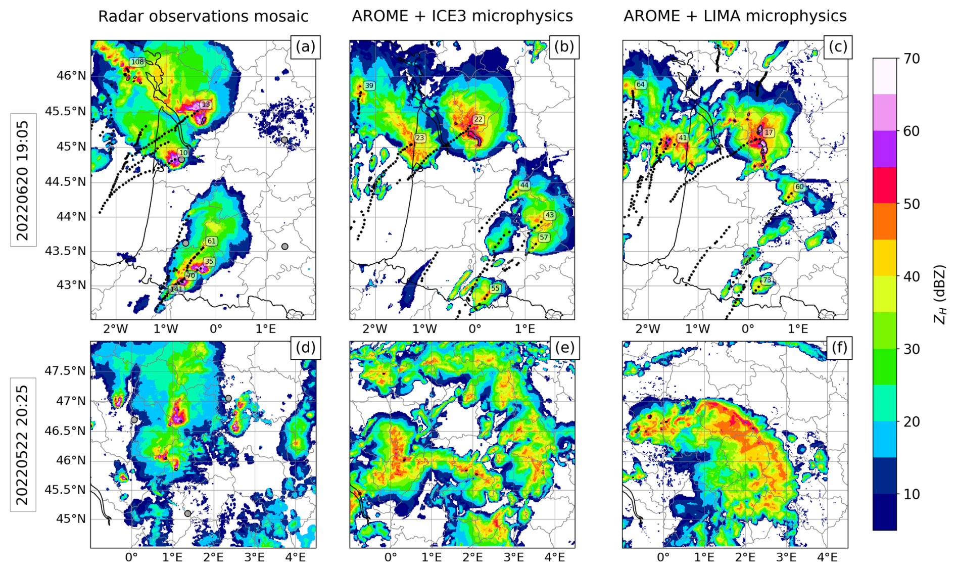
Figure 1Maximum reflectivity over the vertical () for two observed (a, d) and forecasted convective events, at one time instant, with the ICE3 (b, e) and LIMA (c, f) microphysics schemes, respectively. For the first event (a, b, c) an example of the tracking algorithm is displayed. Each black dot represents the past positions of the cell centroids. The label associated with the closest dot corresponds to the number of the identified cell feature at the time step shown. Each detected ZDR column is materialized with a black contour. A demonstration of the tracking is available (David, 2025e).
3.3.3 ZDR column tracking
ZDRCs are small and fleeting objects, making them challenging to track. As for the cell tracking, a detection of the columns is applied to the ZDRC field (in meters) obtained from the algorithm described in Sect. 3.2. All ZDRCs greater than 500 m are detected, and their respective areal extents are determined through the tobac segmentation process. Then, the linking of the ZDRCs centroids is performed with a search radius of 15 km and a memory of four time steps. In the specific case of ZDRCs, the memory parameter has proven to be very useful, as features are allowed to vanish for a certain number of time steps (here four time steps, i.e., 20 min) and still get linked into a trajectory by keeping the same object identifier. Finally, to optimize their tracking, ZDRCs have been spatially linked to the identified cells by matching the ZDRC centroid to the cell footprint at each time step.
This section presents the results obtained from the 34 selected convective days in 2022. A standard model evaluation is conducted based on accumulated precipitation in Sect. 4.1. Then, the evaluation is focused on storm core objects, whose characteristics are investigated in Sect. 4.2, and comparisons between observed and simulated polarimetric fields are performed in Sect. 4.3. Finally, the evaluation is focused on ZDR column objects in Sect. 4.4.
4.1 Precipitation
In an effort to objectively evaluate forecasts with respect to observations, skill measures are often computed. Such measures are based on counting observation–forecast “yes–no” pairs to fill in a 2×2 contingency table that records hits, correct negatives, false positives, and misses. Then, metrics to evaluate the model performance are generated.
In this section, simulated accumulations of precipitation are compared with ANTILOPE QPE, used as an observational reference (see Sect. 2.2), on the whole French metropolitan domain and over the same time period. The comparison is performed on a daily basis, over the 34 convective days, and restricted to time periods encompassing precipitating events. The considered events are listed in Table A1. For each day, the aggregation period (for both observations and forecasts) runs from the beginning of the first event to the end of the last event if multiple events occurred on that day. For instance, two significant events occurred on 3 June 2022: one from 15:00 to 21:00 UTC in southwest France and the other one between 16:00 and 22:00 UTC in eastern France. Thus, the total time period considered for the aggregation of cumulative precipitation for this day over France (hereafter referred to as RRtot) is from 15:00 to 22:00 UTC (7 h). For days with only one event listed, the aggregation period corresponds to the duration of the observed event. Four dates are taken into account twice to compute the statistics, in this section only, as the initialization hours of the forecasts are different between the events. These dates are mentioned in bold in Table A1. Indeed, it is not possible to aggregate hourly precipitation issued from different AROME runs. In this specific case (same day but not same run), the authors have ensured that there is no temporal or spatial overlap between the events. Consequently, the number of days considered in this section is artificially increased to 38 (34 + 4).
To fill in the contingency table, the domain has been divided into 50 × 50 km boxes. First, the 99th percentile of each box has been calculated for simulated and observed RRtot. This percentile has been chosen (rather than, e.g., the median) in order to focus the verification on the ability of the model to accurately forecast the largest total precipitation accumulations. A set of precipitation thresholds is applied to these RRtot box percentiles, yielding “yes–no” pairs of forecasts and observations that are used to construct the contingency tables (one per accumulation threshold). The tables are summarized by the following scores: the probability of detection (POD; Swets, 1986), the false alarm ratio (FAR; Donaldson et al., 1975), and the Heidke skill score (HSS; Heidke, 1926; Murphy and Daan, 1985). These scores are used to compare the forecast performance of the ICE3 one-moment microphysics scheme with the partially two-moment LIMA microphysics scheme (Fig. 2). Additionally, a bootstrap test is performed using the scores' differences from all 38 cases to determine if the differences between LIMA and ICE3 are significant.
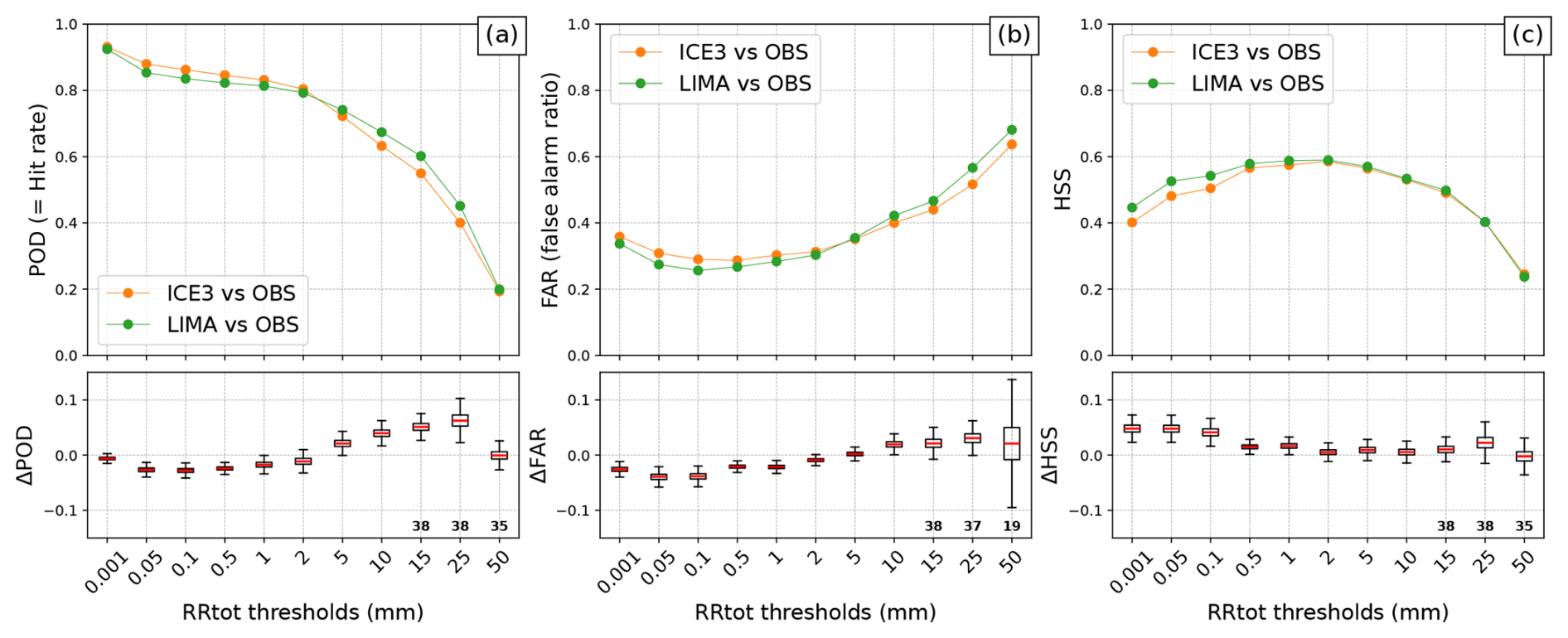
Figure 2POD (a), FAR (b), and HSS (c) for precipitation accumulation forecasts with AROME using ICE3 (orange curves) or LIMA microphysics (green curves). The ANTILOPE QPE is the used as a precipitation accumulation reference. Scores are computed using the 99th percentile within 50 km2 boxes of precipitation accumulation. For each rain rate threshold and score, the distributions from the bootstrap of the score differences between LIMA and ICE3 (Δ) are shown with box plots. The median is displayed in red. Whiskers indicate the 5th and 95th percentiles of the distribution. For the highest thresholds, the number of days involved in the bootstrap is written in bold.
The HSS, which measures the fractional improvement of the forecast over a randomly selected forecast, is presented in Fig. 2c. At the lowest thresholds (RRtot < 2 mm), the HSS is greater for LIMA than ICE3, meaning that LIMA produces better forecasts. This improvement is significant, despite a lower hit rate, which is compensated for by a lower false alarm ratio (Fig. 2a, b). Regardless of the microphysics, the best forecasts are obtained at intermediate thresholds (RRtot = 1–2 mm), where the HSS is maximum (Fig. 2c). There is no significant difference between the two schemes, since the bootstrap confidence intervals are centered close to 0. At the highest thresholds (RRtot > 2 mm), the HSS decreases in both schemes, and LIMA's POD becomes significantly better than ICE3 (Fig. 2a). The POD improvement comes at the expense of higher false alarms (Fig. 2b) so that there is no significant difference in terms of HSS. On average, AROME tends to slightly underpredict the frequency of the strongest thunderstorms (not shown). Hence, the ICE3 and LIMA schemes have similar performance in terms of heavy precipitation forecasts.
4.2 Cell characteristics
Although precipitation scores offer some insight into the forecast performance, they can be difficult to interpret in terms of storm behavior. Indeed, this standard approach is influenced by the location and timing of the storms, thereby rendering any direct comparison of multiple storm objects a challenging undertaking. An object-based approach provides a deeper assessment of cell characteristics, resulting in a more straightforward comparison between observations and simulations, as illustrated below. In particular, comparisons remain valid even when the spatiotemporal structures of the objects are not identical. The object framework is complementary to the standard framework, and together they allow further analysis. Based on the storm objects defined in Sect. 3.3.2, this section will focus on three key features of a cell: its convective core area, its duration, and its maximum intensity.
To analyze the intensity of storms in terms of objects, the size distribution of all detected convective cores is first studied and presented in Fig. 3. In this figure, the time dimension is ignored; i.e., each core contributes as many times as the number of time steps during which it exists. Figure 3 shows that the small cores (defined here as being smaller than 50 km2) are too rarely simulated. This behavior is expected, as Ricard et al. (2013) diagnosed the effective resolution of AROME to be of the order of 9–10Δx, where Δx = 1.3 km is the grid resolution. This implies that objects of size smaller than 136–169 km2 cannot be fully resolved by AROME. In the observations, small cores are associated with reflectivity values ranging from 40 to 68 dBZ (not shown), which correspond to emerging/dying cells or weak isolated storms. In the ICE3 and LIMA forecasts, small cores are linked to values of ZH ≤ 55 dBZ and ZH ≤ 64 dBZ, respectively (not shown). On the other hand, the largest convective cores (defined here as being greater than 1000 km2) are overestimated in frequency by both forecast models. The same statement applies to the envelopes of the detected cells (histogram not shown). It is in agreement with Brousseau et al. (2016), who showed that AROME tends to overestimate the objects' sizes over a sample of 48 convective days in 2012. Stein et al. (2015) also observed an overestimation of the horizontal size of the cells simulated by the Met Office Unified Model (of horizontal resolution 1.5 km).
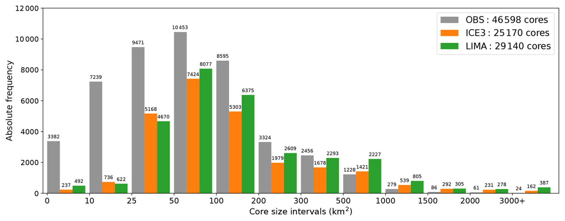
Figure 3Size distribution of detected convective cores ( ≥ 40 dBZ) over all time steps for observations (gray bars) and simulations with ICE3 (orange) and LIMA microphysics (green). The total number of detected cores is listed in the legend. The count of each bin is displayed above the bars.
As a second key characteristic, the temporal evolution of the thunderstorms is studied. Over the 44 studied events listed in Table A1, a total of 3177 cells were observed and detected, while 1506 cells were simulated with ICE3 microphysics and 1776 with LIMA microphysics. The mean cell lifespan in our observation sample is approximately 75 min, while simulated cells last on average 82 min with LIMA and 84 min with ICE3. Figure 4 shows that there is an underestimation in the number of short-lived cells, defined here as cells that last less than 60 min from the birth to the death of the convective core. These short-lived cells make up 40 % of the observational dataset, against 33 % and 34 % in the ICE3 and LIMA forecast datasets, respectively. During the mature stage of these observed short-lived cells, at least 65 % of them had an observed convective core size that never exceeded 50 km2, whereas in the forecasts, only 55 % of the ICE3 and LIMA cells met this condition throughout the mature stage (not shown). The number of convective cells, in particular the weakest ones, was also underestimated in convective-scale simulations with different microphysics schemes in the study of Köcher et al. (2022) as well as in Brousseau et al. (2016) with AROME and ICE3 microphysics. The total rainfall over all cases reached 1.40×10⁵ m3 for LIMA and 1.29×10⁵ m3 for ICE3, while only 0.95×10⁴ m3 of rain has been observed (not shown). This is consistent with the overestimation of size and lifespan we observed for the detected cells. The difference between the observed and simulated amount of convective precipitation is a known positive bias of the AROME model (Stein, 2011). These findings demonstrate that neither of the microphysics schemes considered is clearly superior in terms of the size and lifetime of the convective cells, which is in agreement with the precipitation scores.
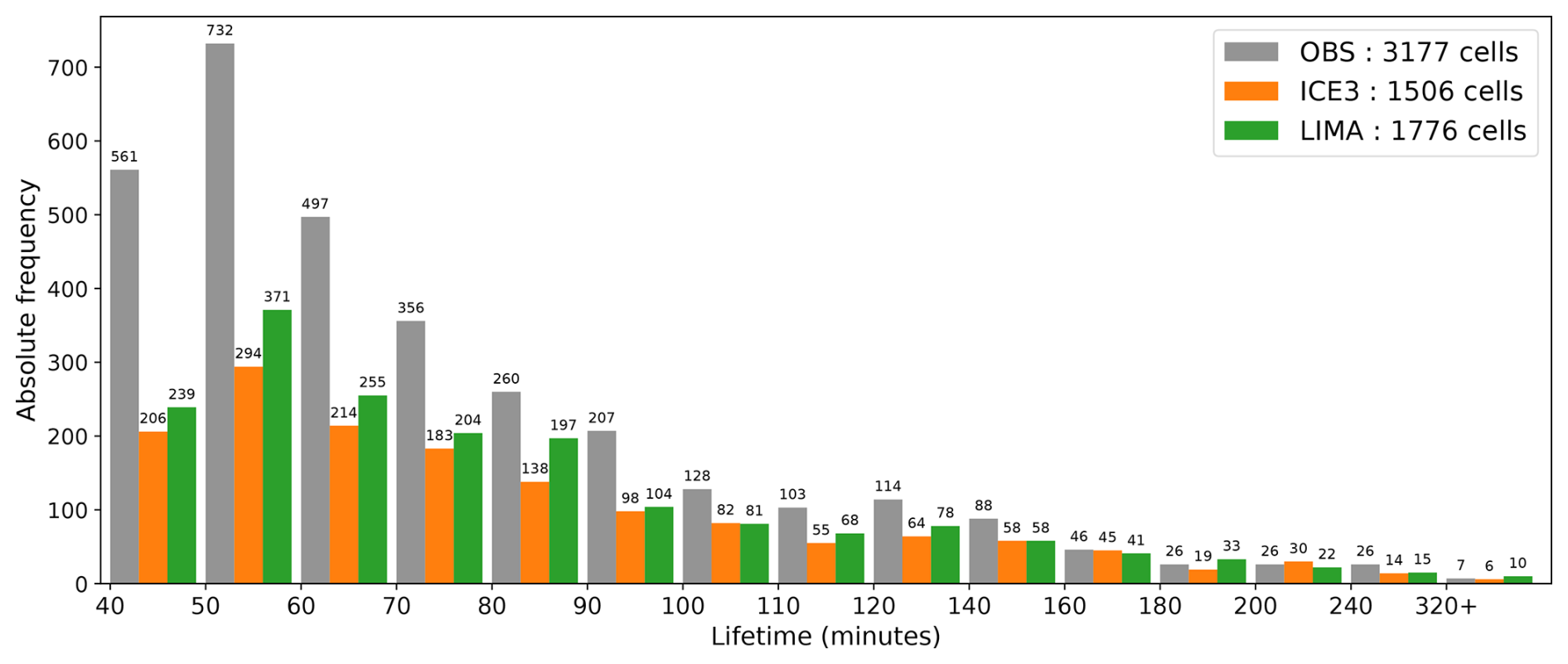
Figure 4Lifetime distribution of detected cells over all convective events for observations (gray bars) and simulations with ICE3 (orange) and LIMA microphysics (green). The total number of detected cells is listed in the legend. The count of each bin is displayed above the bars.
Another key parameter monitored by forecasters is , the maximum reflectivity within the storm, which is closely related to storm intensity. A study of the distribution within each cell core object is proposed herein, with Fig. 5 showing the distribution of the maximum reflectivity a simulated cell can reach compared to its observed counterpart. Please note that reflectivities below 36 dBZ cannot exist due to the tracking thresholds of at least 36 dBZ. Since the microphysics schemes considered do not have a distinct hail class, the observation curve (in black, Fig. 5) has been complemented by another curve (in gray) that only includes observed cores not associated with medium hail (5–20 mm) or large hail (> 20 mm) as detected by the A13 radar hydrometeor classification algorithm (see Appendix C of Forcadell et al., 2024). Comparing these curves shows that the highest reflectivities are associated with hail detection; in particular, the gray curve drops to zero above 65 dBZ, while the black curve does not. The distribution peaks of the ICE3 and LIMA forecasts are similarly located at a reflectivity of 48.5 dBZ, which is lower than in the observations (around 55 dBZ). The distribution is narrower in the ICE3 forecasts (orange curve) than in the observations, whereas the LIMA distribution (green curve) is broader. Figure 5 also shows that for cores of comprised between 58 and 68 dBZ, LIMA differs mainly from ICE3 in its ability to simulate high reflectivity. Indeed, over this interval, the LIMA distribution is more consistent with the observations, a conclusion that is even more pronounced when excluding observations associated with radar-detected hail. The underestimation of the highest reflectivities in the model (in particular with ICE3 microphysics) was already demonstrated by Brousseau et al. (2016) within 31 and 41 dBZ reflectivity contour objects (see their Fig. 8, panels e and f). Cores of the weakest intensities ( between 35 and 45 dBZ in Fig. 5) are less frequent in the forecasts, regardless of the microphysics involved. This suggests that storms develop and/or die faster in simulations than in observations.
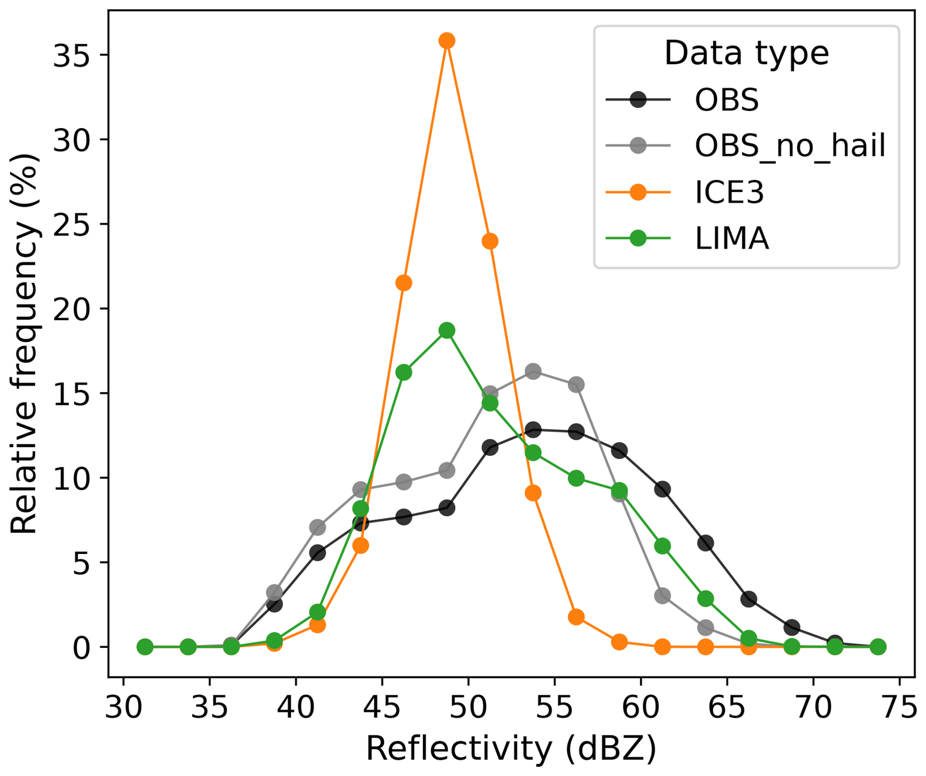
Figure 5Distribution of the cell maximum reflectivity inside the convective core for simulations with ICE3 (orange curve) and LIMA (green curve). The distribution of all observations is displayed in black. The gray curve corresponds to all observations that are not linked to radar-detected hail. The time dimension is omitted. Results are given in terms of relative frequency: each bin value has been divided by the total number of values (see Fig. 4 legend) for each data series and multiplied by 100.
4.3 3D analysis of polarimetric fields
This section analyses the three-dimensional distribution of the reflectivity ZH, the differential reflectivity ZDR, and the specific differential phase KDP inside the storm's convective cores (previously defined as ≥ 40 dBZ). Pre-processed polarimetric observations (see Sect. 3.1) of these variables are obtained from dual-polarization radars of the Météo-France network. The same variables are simulated by applying the radar forward operator (described in Sect. 2.4) to AROME forecasts coupled with either ICE3 or LIMA microphysics. Contoured frequency by altitude diagrams (CFADs; Yuter and Houze, 1995) have been generated for observed and simulated polarimetric fields, inside all detected cores and over all time steps (Fig. 6a, b, and c). In order to gain insight into the processes occurring over the vertical, CFADs are also generated for ICE3 (Fig. 6d) and LIMA (Fig. 6e) hydrometeor contents. The analysis of these results revealed three distinctive regions, which are analyzed separately below.
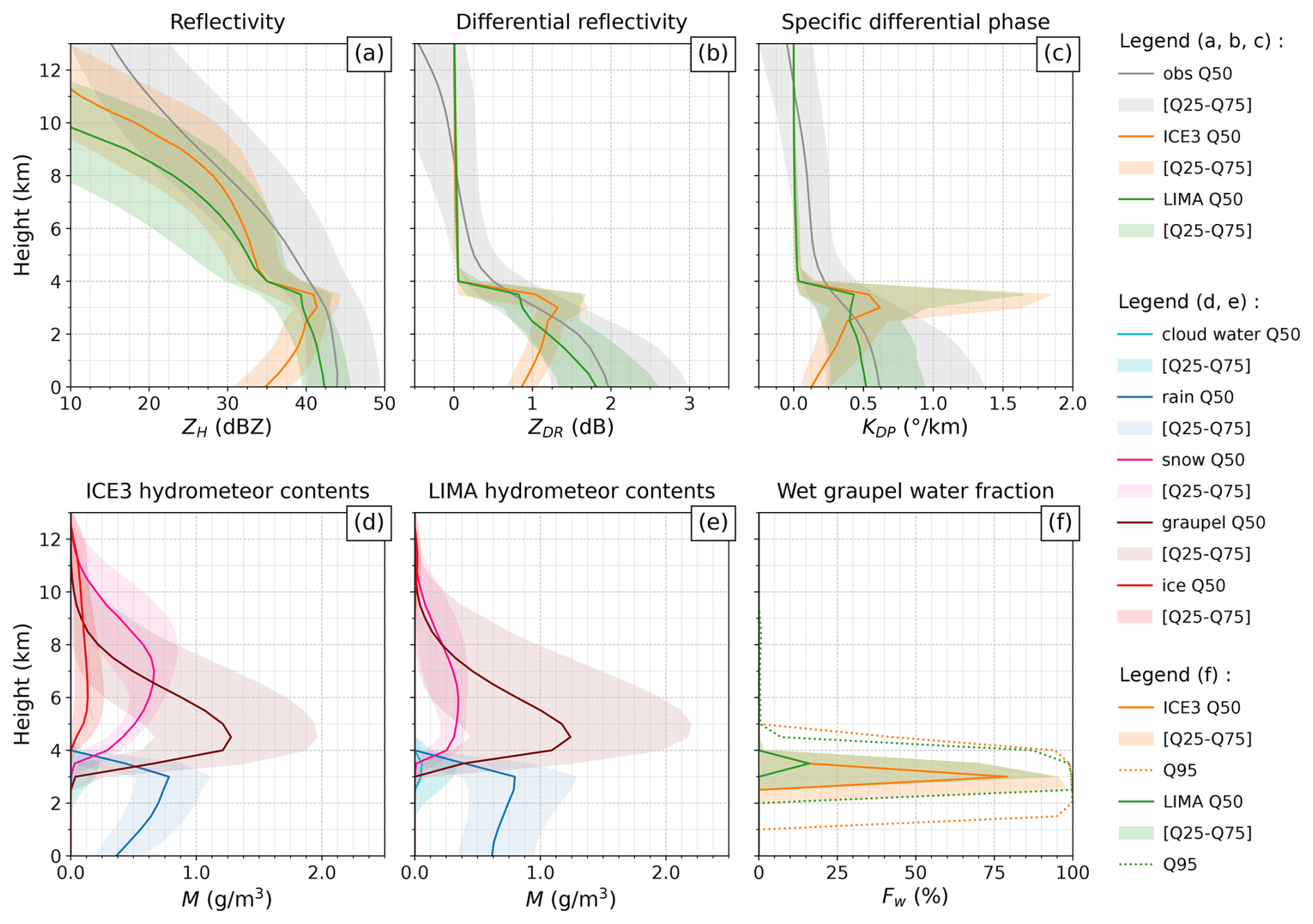
Figure 6CFADs of measured and simulated reflectivity (a), differential reflectivity (b), and specific differential phase (c) inside all detected cell cores ( ≥ 40 dBZ). CFADs of the corresponding hydrometeor contents (expressed in g m−3) for simulations with AROME coupled to ICE3 (d) or LIMA (e) microphysics scheme. CFAD of the liquid water fraction of the wet graupel within convective cores (f) for simulations with ICE3 (orange) or LIMA (green). For all panels, plain lines correspond to the median, and the interval of the 25th and 75th percentiles of the distributions is displayed in lighter colors behind each curve. For panel (f), the 95th percentile is shown with dotted lines. Altitudes are given in kilometers above ground level (a.g.l.).
4.3.1 Low levels
The first region of interest is located under the melting layer, below 3 km height, where most of the observed reflectivities ranged from 40 to 50 dBZ. In this area, ZH (Fig. 6a), ZDR (Fig. 6b), and KDP (Fig. 6c) decrease with altitude in the LIMA simulations (in green), as observed (in gray), but the distributions are slightly underestimated. In contrast, ICE3 simulations (in orange) show increasing values with height, resulting in strong underestimations at ground level, where the differences between observed and simulated medians are 18 dBZ, 1.2 dB, and 0.5° km−1, respectively. However, in simulations with both ICE3 and LIMA, the rain content increases with height (dark blue curves in Fig. 6d and e), with a steeper slope for ICE3. Figure 6b shows that raindrops are smaller with ICE3, as indicated by the ZDR values, which decrease towards the ground. Indeed, ZDR is an indicator of the raindrop mean volume diameter (Seliga and Bringi, 1976) and is independent of the drop concentration. Similarly, the KDP values in ICE3 simulations decrease towards the ground (Fig. 6c), as this variable is sensitive to the amount of liquid water. More specifically, Jameson (1985) demonstrated that KDP can be linked to the product of liquid water content and the mass-weighted mean raindrop axis ratio, which explains the different behavior of LIMA in Fig. 6c. Indeed, when temperatures are above 0 °C, raindrops evaporate as they fall to the surface. The evaporation process seems to be more efficient in the ICE3 microphysics than in the LIMA microphysics. An explanation for this apparent discrepancy is that LIMA allows the simulation of bigger and more oblate raindrops under the melting layer because its rain content and number concentration are prognostic. Thus, in similar conditions of humidity, the smaller raindrops in ICE3 will evaporate faster than those in LIMA, leading to a rapid decrease in the rain content in ICE3.
In summary, the rain characteristics are better simulated with the two-moment representation in LIMA, and vertical profiles of ZH, ZDR, and KDP are in stronger agreement with the observations below the melting layer. Moreover, the Q25–Q75 interval shows that the ICE3 ZDR and KDP values have less spread than the observations and the LIMA simulations, the latter having an interval width closer to that observed.
4.3.2 Bright-band region
The bright-band region (hereafter BB) is a radar signature which highlights the layer where frozen hydrometeors melt to form rain. In our simulations the BB is visible at altitudes between approximately 3 and 3.5 km within convective core objects (according to the median curves in Fig. 6a, b, and c), but not in the observations. Although the BB is not always visible in observed convective areas, other effects such as smoothing due to beam broadening (see Meischner et al., 2004; Sect. 2.4.3 and Fig. 10.25 of Ryzhkov and Zrnic, 2019) or the interpolations used to map the radar data onto a 3D Cartesian grid can explain the absence of observed BB. The microphysics schemes used in this study do not have prognostic melting species, but a wet graupel species is artificially diagnosed using the enhanced melting scheme implemented in the radar forward operator (see Sect. 2.4 and Appendix B). Figure 6f shows the liquid water fraction Fw within the wet graupel in the detected convective areas. The depth of the layer where its 95th percentile is nonzero shows that wet graupel is present in a broader layer in ICE3 than in LIMA. It can also be seen that the peak of the Fw median reaches higher values in ICE3: at 3 km height, 50 % of the ICE3 wet graupel content is at least 75 % melted, whereas at 3.5 km height, 50 % of the LIMA wet graupel content is at most 15 % melted. These results explain why a more pronounced BB can be seen in ICE3 simulations, especially in terms of ZDR and KDP CFADs (Fig. 6b and c), because these variables are sensitive to the oblateness and liquid water content of the particles.
The differences found between ICE3 and LIMA (in Fw and the BB intensity) may be associated with the broader distribution in both rain and graupel contents, as well as the bigger cloud droplet content in LIMA, in the BB region. However, to better assess the representation of the BB by both microphysics schemes, an evaluation of stratiform events, where the BB is clearly visible in observations, is required (as in Shrestha et al., 2022a).
4.3.3 Above the melting layer
Just above the bright-band region (around 4 km), the graupel particles are mostly dry since their liquid water fraction is close to zero (Fig. 6f). Despite significant snow and graupel contents, Fig. 6 shows that simulated ZDR and KDP drop to zero at levels with low to no rain content, whereas the median of observations remains positive until 8 km for ZDR and 11 km for KDP. This is consistent with Köcher et al. (2022) and Shrestha et al. (2022b). A weak positive ZDR value can be associated with dry snow or graupel (which can potentially start to melt) and aggregated ice crystals, while a negative KDP may be the sign of vertically oriented ice crystals within a strong electric field (Ryzhkov and Zrnić, 2007; Hubbert et al., 2014). In simulations, only pristine ice, snow, and dry graupel are available at higher altitudes (Fig. 6d and e). However, approximations made in the forward operator result in null values of ZDR and KDP in pristine ice crystals, which are modeled as spheres because of their random orientation (as in Caumont et al., 2006). Very low values of simulated ZDR and KDP could be due to a density and/or dielectric constant too low for dry snow and dry graupel. A more exhaustive discussion of these aspects can be found in Sect. 5.2.
On the other hand, observed reflectivities decrease more smoothly with altitude (Fig. 6a). This phenomenon indicates that ice growth processes are underway. Independently of the microphysics, all forecasts showed a sudden decrease in the reflectivity between 3.5 and 4 km height. Then, at higher altitudes, both microphysics schemes underestimated the reflectivities (LIMA more than ICE3). Compared with the work of Köcher et al. (2022), most of the analyzed microphysics schemes overestimated ZH values above the melting layer. According to the authors, this could be explained either by an overestimation of graupel content or the particle size or the density set in the forward operator. However, it can be seen in Fig. 6d and e that the main difference between ICE3 and LIMA above the melting layer is the distribution of the ice and snow contents, whereas the median graupel content is relatively similar. This may be linked to the limitations of the version of LIMA used in this study. Indeed, ice production is limited by the availability of ice nuclei, and the conversion to snow occurs as soon as pristine ice crystals grow larger than 125 µm in diameter. Thus, ice tends to disappear rapidly, resulting in lower snow contents than in ICE3 and consequently lower reflectivity values. The reader can find in Appendix C an illustration of the A16 forward operator sensitivity to different hydrometeor contents for one-moment species (e.g., snow and ice; see Fig. C1) or for a two-moment ice class (Fig. C3). Recent improvements in LIMA (Taufour et al., 2024), such as the implementation of secondary ice production mechanisms, may improve the representation of the upper part of the convective clouds. Although simulations with ICE3 microphysics give better ZH values, overall a negative bias still persists when the snow and ice contents are insufficiently represented in the microphysics.
4.4 ZDR columns
The use of dual-polarization observations coupled to an object-based detection allows the identification of specific signatures in thunderstorms. This section is focused on the ZDR column (ZDRC), which highlights the location of storm updrafts and indicates the presence of supercooled liquid water being lofted above the environmental freezing level. This signature has raised interest in the scientific community, notably for nowcasting or assimilation purposes (Kuster et al., 2019, 2020; Carlin et al., 2017). Nevertheless, using ZDRCs in such contexts requires them to be correctly simulated by forecast models. This section will concentrate on the main characteristics of a ZDRC: its depth and horizontal extension. As a ZDRC is inherently linked to a convective cell, its temporal evolution will also be examined, as well as its 3D structure.
The first interesting feature about the ZDRC is its maximum height, counted from the 0 °C isotherm level, and hereafter referred to as column depth. A deep column can be the sign of a very intense updraft, with an increased risk of producing large hailstones, due to a longer residency time above the melting layer, in a zone with enhanced supercooled liquid water content (Kumjian et al., 2021). Figure 7 shows that 69 % of the observed columns had a depth of 0 to 2 km above the 0 °C isotherm, whereas 31 % of the columns simulated with ICE3 are included in this interval versus 89 % for LIMA. Columns with a depth greater than 4 km account for 3.1 % of the observed sample and for 2.6 % of the ICE3 sample, which is similar. On the other hand, LIMA only simulated two columns with a maximum depth of 4 km. Although the LIMA simulations approximately generated the same total number of columns as the observations (see the legend in Fig. 7), the shape of the observed column depth distribution is not accurately simulated by the two microphysics schemes.
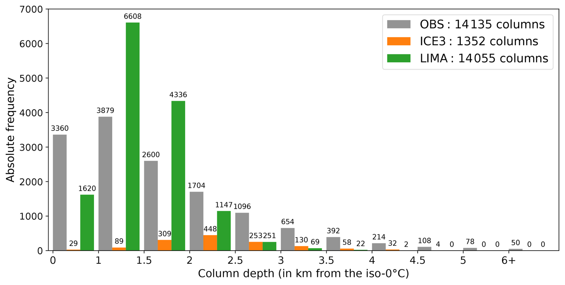
Figure 7Distribution of ZDR column maximum depth over all time steps for observations (gray bars) and simulations with ICE3 (orange) and LIMA microphysics (green). The total number of detected columns is listed in the legend. The count of each bin is displayed above the bars.
An analysis of the 3D distribution of the differential reflectivity and the hydrometeor contents over the vertical, illustrated by the CFADs within ZDRC objects in Fig. 8, shows one similarity with the results found for the storm core objects: simulated ZDR values (Fig. 8a) rapidly decrease above the freezing level as well as the rain content (dark blue curves in Fig. 8b and c). While dry graupel contents (brown curves) are still significant at this level for both microphysics schemes, the distribution of the liquid water fraction within the wet graupel (Fig. 8d) shows discrepancies between the two schemes. Indeed, within the ZDRCs, rain reached higher altitudes with ICE3 (median at 6 km in Fig. 8b) than with LIMA (median at 5 km in Fig. 8c), although more cloud water (light blue) is available for LIMA (with the 75th percentile going up to 6 km). The distribution of ZDR in Fig. 8a provides additional evidence of the ability of ICE3 to produce deep ZDRCs. However, it can be seen that ZDR values are only slightly larger than 2 dB, the threshold chosen in this study for the ZDRC algorithm. This strict thresholding may penalize the detection of ZDRCs in ICE3 simulations and encourage the selection of only the most intense updrafts, resulting in a low number of detected columns but of a greater depth. In light of the available cloud water in the LIMA simulations, it may be beneficial to consider incorporating this content into the forward operator melting scheme (e.g., taking into account this content in the computation of Fw), with the aim of producing slightly higher ZDRCs with LIMA microphysics. Another discrepancy between ICE3 and LIMA is the ZDR signal under 4 km. While ZDR values are underestimated in ICE3 compared to the observation (Fig. 8a), ZDR is overestimated with LIMA, whereas the rain content is clearly lower than with ICE3 (Fig. 8b and c). Compared to the observations, such high values of ZDR could be the consequence of a size sorting process that is too strong within the ZDRCs simulated by LIMA, producing raindrops that are too large (and oblate). Similarly, Putnam et al. (2017) and Köcher et al. (2022) found overestimated ZDR values in rain with a two-moment microphysics, in particular with the Morrison and Thompson schemes using WRF simulations (Skamarock et al., 2008). It should be noted, however, that the overestimation of simulated ZDR in this study is confined to the ZDRC objects and not seen in the convective cores where the ZDR values are very close to the observation and slightly underestimated as discussed in Sect. 4.3 and shown in Fig. 6b. A likely explanation is that detected convective core objects also include some of the downdraft regions, where raindrops are no longer lifted by an updraft and subsequently fall, unlike updraft regions targeted by the ZDRC objects. Moreover, the size sorting usually occurs at low levels, whereas the overestimated ZDR values here are mainly located around 3 km, further supporting the hypothesis of an updraft-related process. In the microphysics schemes, the size of the raindrops produced by the melting of the graupel is arbitrarily set. Adjusting this parameter could also be a way to reduce the ZDR overestimation just below the melting level.
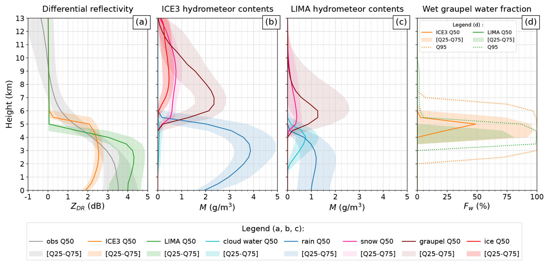
Figure 8CFAD of differential reflectivity (a) and CFAD of hydrometeor contents (expressed in g m−3) in simulations with AROME coupled to ICE3 (b) and LIMA microphysics (c) inside all detected ZDR columns. Similarly to panel (a), panel (d) shows the liquid water fraction within the wet graupel of ICE3 and LIMA. Plain lines correspond to the median, and the interval of the 25th and 75th percentiles of the distributions is displayed in lighter colors behind each curve. Altitudes are given in kilometers above ground level (a.g.l.).
The study of Kumjian et al. (2021) further highlighted the relevance of the column area as a parameter linked to storm intensification. Indeed, a large column may be indicative of a substantial quantity of supercooled lifted raindrops, which could result in an elevated production of hailstones of small to moderate size. Figure 9 shows the distribution of the column area. Approximately 64 % of the observed columns are small features (less than 15 km2), which is a known characteristic of ZDRC. Simulations with ICE3 demonstrate satisfactory results in terms of proportion, with 69 % of the ZDRC being small features against 67 % with LIMA. In Shrestha et al. (2022b), the TSMP model (Gasper et al., 2014; Shrestha and Simmer, 2020) coupled with a two-moment bulk microphysics scheme (Seifert and Beheng, 2006) was found to underestimate the area of ZDRCs. While in the present study the area of the ZDRCs is not underestimated in terms of proportion, regardless of the microphysics, ICE3 simulations nevertheless produced an insufficient number of ZRDCs in comparison to LIMA simulations. The accuracy of LIMA regarding the ZDRC is noteworthy in terms of both area distribution and absolute number.
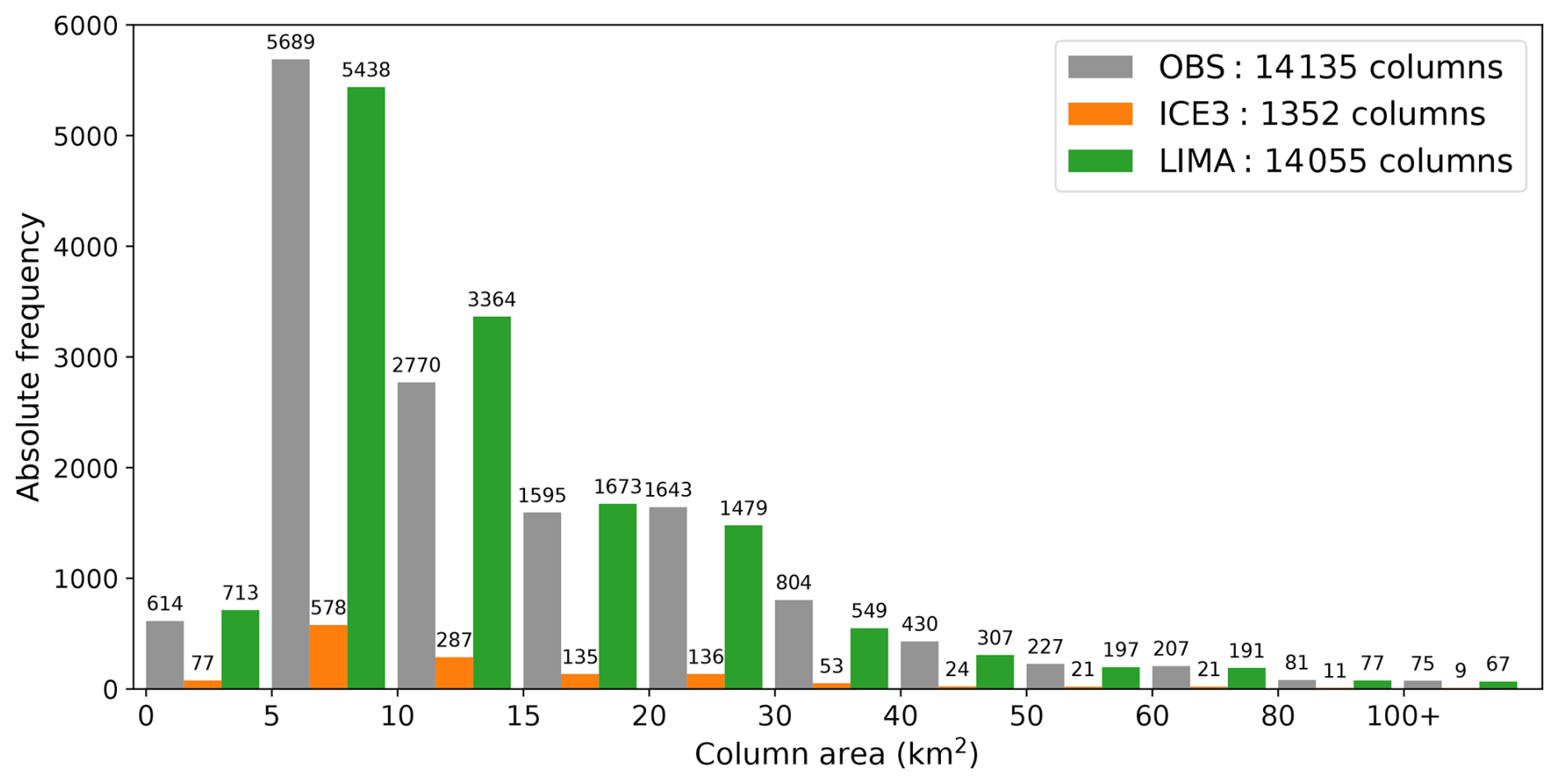
Figure 9Area distribution of ZDR columns over all time steps for observations (gray bars) and simulations with ICE3 (orange) and LIMA microphysics (green). The total number of detected columns is listed in the legend. The count of each bin is displayed above the bars.
As the ZDRC is a proxy for the updraft, it is often observed as soon as the storm core develops. Thus, the first occurrence of a ZDRC is an important marker of the life cycle of the associated storm cell. In this study, 43.8 % of the observed cells were associated with a ZDRC against 26.8 % for ICE3 and 44.5 % for LIMA. The box plot presented in Fig. 10 shows the distribution of the first ZDRC occurrence time relative to the lifetime of the cell to which it belongs. It is expressed as a percentage, where 0 % corresponds to the emergence of the convective core and 100 % to its death. First, it can be noticed that the 5th and the 25th percentiles are coincident and equal to 0 % both in simulations with LIMA and in the observations. This means that in 25 % of the analyzed events, the ZDRC is formed and detected at the same time as the convective core. The relative lifetime of the cell can be approximately divided as follows: [0 %–20 %] developing stage, [20 %–80 %] mature stage, [80 %–100 %] dissipating stage. At least half of the first ZDRC detections occur during the early cell development stage. The same behavior is observed in forecasts coupled with LIMA microphysics, but not with ICE3, whose median is around 32 % of the relative cell lifetime, meaning that more than 50 % of the columns are detected during the mature and dissipating stage. Although it is uncommon for the initial ZDRC to be observed during the dissipating stage of the cell (gray box plot, Fig. 10), it occurred much more frequently with ICE3, as shown by the broader spread and the absence of outliers in its time distribution (orange box plot, Fig. 10). Some delay in the ICE3 ZDRC identification may be attributed to the strict thresholding of the detection algorithm (see Sect. 3.2). One can assume that, in the case where ICE3-detected updrafts are only the strongest, it should counterbalance this effect, since the deepest columns can be expected to occur before the dissipating stage or at the beginning of the mature stage. However, it should be noted that, as seen in Fig. 8b, ICE3 requires very high rain contents to simulate significant ZDR values because in a one-moment scheme, the number concentration is unable to vary independently of the content.
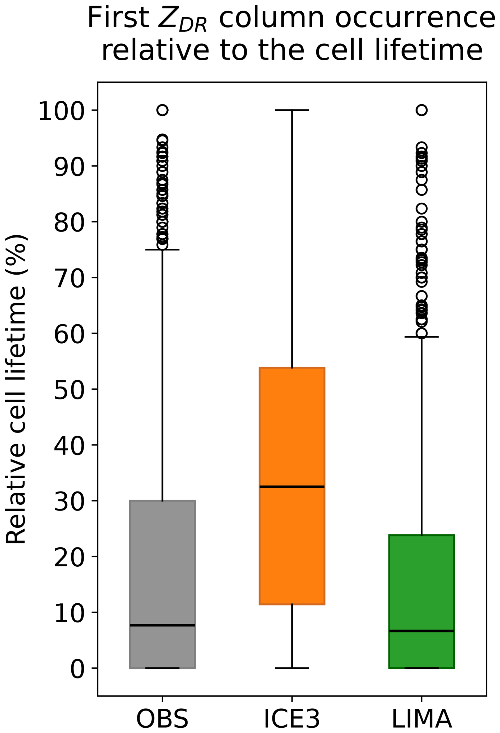
Figure 10First ZDR column occurrence relative to the cell lifetime for observations (gray bars) and simulations with ICE3 (orange) and LIMA microphysics (green). The cell lifetime is expressed in percentage, with 0 % being the emergence of the convective core and 100 % its death. The median is shown with the thick black line. Whiskers correspond to the 25th and 75th percentiles. Outliers are displayed as dark circles.
To conclude, the lack of rain above the freezing level within LIMA simulations has a direct impact on the liquid water fraction in the melting scheme (wet graupel), despite the presence of liquid water at these altitudes (cloud water). Moreover, the depth of the ZDRC is not accurately reproduced by either microphysics scheme, but the ZDRC area, which is a more significant feature, is well reproduced by both schemes in terms of relative distribution. Only LIMA was able to reproduce the correct amount of ZDRC with a precise area distribution. Finally, the temporal evolution of the ZDRC appears to be accurately forecasted by AROME in conjunction with the LIMA scheme, lending further credibility to this scheme. These findings are highly encouraging with regard to the potential use of LIMA, in particular for the column area feature used with a strict detection threshold.
Although the simulations performed with LIMA showed remarkable agreement with the observations for rain in the convective cores and a very realistic area distribution and number of ZDRC columns, the present work also revealed discrepancies between observed and synthetic radar data simulated with the A16 forward operator. These discrepancies may be introduced by the radar forward operator, the microphysics schemes, the ZDR column detection method, or a combination of the three. This section is intended as an open discussion about the realistic expectations, constraints, and possible areas for improvement.
5.1 Mixed phase parameterization
The results of this study have emphasized the challenges of parameterizing the mixed phase. These issues are characterized by an overestimation of the bright band (BB) in the simulations within convective regions, as well as a notably low amount of rain at negative temperatures in both convective cores and ZDRC objects, which is particularly pronounced with LIMA microphysics.
To improve the melting layer simulated by the forward operator, it may be beneficial to consider modifying the estimation of the mixed phase, as various parameterizations exist in the literature. For example, Jung et al. (2008) assumed the existence of a mixed phase when dry snow and rain coexist, thus converting a certain proportion of rain and snow to wet snow. On the other hand, in the A16 operator used here, the wet species are computed from the graupel and rain content when they coexist, and a wet graupel class is created by consuming the entire graupel content only. Wolfensberger and Berne (2018) used an alternative parameterization in which wet aggregates and wet graupel exist within the melting layer. Liu et al. (2024) recently proposed a melting model, independent of ambient temperature, that relies on the mixing ratio and number concentration of rain and ice species. Such parameterizations will be tested and compared in a future work.
It is worth remembering that, initially, in the A16 forward operator, a wet graupel class was chosen to stay consistent with the microphysics: in the model, the melting snow content is transferred into the graupel class. Because of this, melting graupel output from the forward operator can be either actual melting graupel or melting snow. If the microphysics scheme cannot be modified, an alternative strategy would be to address the issue directly within the radar forward operator. Therefore, it may be worthwhile to try to differentiate a posteriori melting snow and graupel. In the hydrometeor classification algorithm of Park et al. (2009), a vertical continuity check is performed to distinguish between the convective and stratiform parts of the storm and has proven to improve the level of discrimination between graupel and snow (dry or wet). Given that the ZDRC detection algorithm developed in this paper includes a vertical continuity check, there is the potential to conduct straightforward tests to adapt such a continuity check so that a basic discrimination is applied to both the model and observations. Then, this discrimination could be used by the forward operator to separate wet snow and wet graupel.
As a second area for improvement, the computation of the water fraction within wet species could be modified. In the A16 operator, the liquid water fraction is a function of the graupel and rain content and is equally distributed among the whole particle size distribution. In Dawson et al. (2014) the water fraction is diagnosed with an iterative method. Based on a first guess, up to 90 % of the rain content available is added and distributed into the melting species contents (graupel and/or hail). A critical mass of water that can exist on a melting particle is estimated and integrated over the corresponding PSDs to determine a critical water fraction which is a function of the particle diameter (according to Fig. 2 in Dawson et al., 2014). If the available rain content exceeds this critical water mass value, then this value is used as the next guess of rain content to be added into the melting species contents. In other words, the liquid water fraction varies across the melting particle size distribution.
In pursuit of greater realism, a two-layer spheroid T-matrix code following Ryzhkov et al. (2011) could also be implemented, as ice, air, and water in a mixed phase particle are currently treated either as a matrix or an inclusion, which is known to affect the computation of the dielectric constant. Nevertheless, Ryzhkov et al. (2013) demonstrated that the T-matrix computation for two-layer and uniformly filled spheroids (assuming water as the matrix) yields similar results in terms of radar variables after an integration over all particle sizes. Moreover, this study was focused on the ability of the model to correctly simulate the radar variables within convective cores, which is not adequate to evaluate the melting scheme parameterization. Thus, improvements in the radar forward operator regarding the bright-band signature should be analyzed during stratiform events or, at least, focused on the stratiform parts of the convective storms. Therefore, the A16 forward operator is currently being tested in stratiform environments. While, under the freezing level, realistic polarimetric values were obtained with LIMA, and, with a view to more realistic modeling, it would be valuable to conduct a comparative analysis of the microphysics schemes presented in this work by including a separate hail class, as in this work, hail was included in the graupel class and hence unable to reach the warmer levels of the atmosphere.
5.2 Cold phase modeling
Other challenges have emerged in the cold phase, as simulated ZDR and KDP dropped to almost zero at levels with low to no rain content, despite significant snow and graupel contents. Köcher et al. (2022) and Shrestha et al. (2022b) (hereafter referred to as K22 and S22b) found similar results with different microphysics schemes and radar forward operator parameterizations. Directly above the melting layer, graupel was found to be dominant in both studies. Nevertheless, the aspect ratio of the graupel is assumed to be 1 in K22, while in this study, the aspect ratio is set to 0.8 if the graupel is dry or is determined using the formulas described in Ryzhkov et al. (2011) if the graupel is wet. In S22b the graupel axis ratio follows the same equations as in this study, but parameterizations of snow and ice are different. The axis ratio of cloud ice is set to 0.2, against an axis ratio of 1 here. However, even with a 0.2 axis ratio, near-zero ZDR and KDP values have been found within simulations all along the vertical above the melting layer. According to S22b, deficiencies in the forward operator may play a significant role. Shrestha et al. (2022a) showed, for a stratiform event, that snow was found to dominate above the melting layer. In their study, a variety of snow shapes and orientations were tested, but they were still unable to reproduce the observed polarimetric values at these heights. In K22 an enhanced but not realistic ZDR signal has been produced between 8 and 12 km height, with two of the five microphysics schemes analyzed. These high values were caused by the cloud ice, whose assumed aspect ratio by the forward operator is 0.2.
Part of the underestimation of dual-polarization variables in snow could be due to the (overly) simple representation of aggregates by homogeneous spheroids with the T-matrix method, as suggested by Trömel et al. (2023), based on the study of Schrom and Kumjian (2018). Another method, known as the discrete dipole approximation (or DDA; Purcell and Pennypacker, 1973; Draine, 1988), allows the simulation of more complex geometries. This method decomposes the particles into a collection of subregions, each being small enough to be considered a dipole. With this technique, each single dipole can be arranged to form different and complex shapes of crystals or aggregates. However, the DDA method is computationally expensive due to the necessity of solving a large system of linear equations with a dense matrix. It is not implemented in our current forward operator. Hence, in order to increase the ZDR and KDP values in snow, a modification of the snow density–diameter relationship would be more accessible and could be investigated. Moreover, a riming factor could be included in the snow parameterization, following the formulation of Brandes et al. (2007), as it proved to simulate acceptable values in snow in the study of Carlin and Ryzhkov (2019).
Overall, this work, in conjunction with all previous related studies, shows how hard it is to simulate accurate polarimetric values within and above the melting layer with the diversity of microphysics and forward operator available. Indeed, the ICE3 and LIMA schemes used here simulate very different cloud compositions above the melting layer. ICE3 produced significant quantities of ice crystals, snow, and graupel. LIMA, on the other hand, resulted in almost zero ice crystal contents, much less snow, and a little less graupel than ICE3. These differences were found both within convective objects and ZDRCs and suggest that this lies in the treatment of ice particles in the microphysics. In ICE3, ice crystals can be continuously formed in favorable thermodynamic conditions, whereas in LIMA, ice crystals are formed only when IFN are available. Thus, once IFN are depleted (used to form ice crystals, scavenged by precipitation, etc.), LIMA cannot create new ice crystals. Because of these differences, the pristine ice to snow conversion is based on the ice particle size in LIMA. This process is more efficient than the simple autoconversion process (which is only active for high ice contents) in ICE3. Consequently, pristine ice is quickly consumed in LIMA to form snow that rapidly falls out.
To address this issue, a hybrid configuration of LIMA, using a one-moment representation of pristine ice crystals as in ICE3, coupled to improvements in the snow representation (Wurtz et al., 2021, 2023) was found to have very good results for tropical convection, retaining most of the advantages resulting from the two-moment cloud droplets and raindrops. Another solution would be to use a secondary ice production process (Shrestha et al., 2022a). Such mechanisms (collisional ice breakup and raindrop shattering when freezing) are available in LIMA and have been implemented since the beginning of our study. They proved very efficient at maintaining significant ice and snow contents in convective clouds. However, as long as the ice crystals are modeled as spheres by the forward operator, the ice content will have little or no effect on the simulated ZDR and KDP values, as illustrated by Figs. C1 and C3 of Appendix C. To improve the accuracy of the polarimetric outputs and provide a more realistic representation, ice crystals must be modeled as oblate spheroids (Matrosov et al., 1996). More general improvements of the radar forward operator are underway to better represent the ice phase.
5.3 ZDR columns
Finally, our ZDRC detection methodology has shown its limitations, especially with regard to the 2 dB threshold, which contributed to difficulties in the detection of ZDRCs in ICE3. As previously stated, the choice of a high threshold was a commitment made to avoid false alarms in the observations and hence to establish a trustworthy reference dataset. Thus, this high ZDR threshold combined with a vertical continuity check partly hindered the detection of ZDRCs in simulations with ICE3 microphysics. Recently, Krause and Klaus (2024) published a novel technique to detect ZDRCs on radar data that only rely on a single horizontal level (constant altitude plan projection indicators or CAPPIs) at the −10 °C altitude. Their technique consists of identifying the column base rather than the entire column depth. After filtering the data, the median values of two boxes (a 7 × 7 “outer box” and a 3 × 3 “inner box”) centered on each grid point are compared, yielding the “hotspot” value. Then, any points that exceed the mean hotspot value by more than 1 standard deviation are retained. Not only did this method demonstrate enhanced performance in regions where there is a bias in differential reflectivities, but the approach is also entirely adaptable to the model world. Thus, the detection of ZDRCs in the model would rely on a comparison of each grid point versus the environment, potentially improving the detection in our simulations with ICE3.
As the last point of this discussion, we highlighted the inability of the AROME model, when combined with the ICE3 microphysics, to produce elevated ZDR values in the ZDRCs. Indeed, the detected ZDRCs in the model are essentially due to wet graupel, thanks to the mixed phase parameterization in our forward operator (i.e., the “wet graupel species” is artificially created to replace the model “dry graupel” if rainwater coexists with graupel, even at negative temperatures). The term “melting scheme” may not be appropriate to describe the physical state of the graupel at negative temperatures. In fact, in our representation at such temperatures, the graupel is not melting but is probably surrounded by a coat of supercooled liquid water. An alternative method to simulate ZDRCs could be the implementation of a raindrop freezing process in the forward operator based on Kumjian et al. (2012). As explained in Chap. 7, Sect. 2.5.1 of Ryzhkov and Zrnic (2019), a raindrop freezes from the outside to the inside and can be represented as an ice shell forming around the droplet, with the core being either purely liquid or a mix of water and ice (embedded ice germ). Thus, the use of a matrix/inclusion approach to represent this process is absolutely relevant and could be easily implemented as it is already available in the A16 operator. Nevertheless, given the insufficient amount of supercooled rainwater available in our current microphysics schemes, this method may not be able to produce the expected results.
In this paper, an evaluation of the microphysics of the AROME NWP model was carried out with two different, but complementary, frameworks. Numerical forecasts were compared with observations using a global and an object-based approach. The main objective was to statistically assess the ability of the AROME model to reproduce thunderstorms in terms of intensity, structure, characteristics, and dual-polarization signatures. A related goal was to compare two microphysics schemes against dual-polarization radar observations: the currently operational ICE3 scheme and the LIMA scheme currently under consideration for future implementation. Given the growing interest in the ZDR column in the scientific community due to its potential applications in the fields of nowcasting and data assimilation, this dual-polarization signature was subjected to a careful investigation. To do so, various features were analyzed over a sample of 34 convective days in 2022, and a ZDR column detection and tracking algorithm was implemented. Dual-polarization radar data were extracted from the French metropolitan network. Forecasts were performed with the AROME model coupled to either the ICE3 (one-moment) or LIMA (partially two-moment) microphysics schemes. An enhanced version of the radar forward operator of Augros et al. (2016) was applied to the forecasts to obtain synthetic polarimetric fields.
First, a global approach was used to evaluate accumulated precipitation fields. Statistical measures (POD, FAR, and HSS) were computed for different rain rate thresholds and compared between simulations with ICE3 and LIMA. The only significant improvement occurred for the smallest rain rates, with a slight decrease in the POD and the FAR but a small increase in the HSS for forecasts with LIMA. For the highest rain rate thresholds, LIMA's overall contribution was fairly neutral as the POD and the FAR both increased, and the HSS remained similar to that of ICE3.
An object-based framework was defined to study polarimetric fields and hydrometeor contents within convective areas of the storms. As a first step, the characteristics of convective cores were compared. Our results show that the model, regardless of the microphysics, has difficulties simulating small and short-lived cells, which is a known issue due to the AROME effective resolution of 9 to 10Δx (Δx = 1.3 km). In contrast, larger storms are often overestimated. Secondly, the 3D structure of polarimetric fields was analyzed with contoured frequency by altitude diagrams (CFADs). The use of LIMA microphysics allowed the simulation of high ZH, ZDR, and KDP below the melting layer. This points to a more realistic raindrop size representation thanks to the two-moment component of rain in LIMA. On the other hand, ICE3 (one-moment) raindrops were smaller and, as a consequence, evaporated faster. This caused a reduction of the rain content, which led to a decrease in the ZH, ZDR, and KDP variables near the ground. For both microphysics schemes, the bright band was visible but more pronounced with ICE3. This is mainly due to the creation of a wet graupel species in the radar forward operator, whose liquid water fraction was found to be greater with ICE3 than with LIMA. In the region above the melting layer, both schemes underestimated reflectivities, but ICE3 was more consistent with the observations thanks to a greater amount of snow and pristine ice in the simulations. Nevertheless, simulated ZDR and KDP were found to be null at these altitudes, regardless of the microphysics used. This suggests radar forward operator issues, as (1) pristine ice crystals are currently modeled as spheres, and (2) the snow density and dielectric constant is probably too low so that the non-spheroidal axis ratio of snow has a minimal influence on the resulting signals.
Finally, the main features of the ZDR column objects were also evaluated. The highest ZDR columns were generated exclusively with ICE3. The analysis of the vertical distribution of ZDR within the columns revealed that ICE3 ZDR values barely exceed 2 dB under the melting layer, but such a value is reached for altitudes up to 5 km versus 4.5 km for LIMA. The lack of raindrops above the melting layer in LIMA's ZDR columns can explain part of this discrepancy. An analysis of the temporal occurrence of the first detected ZDR column, with respect to the cell it belongs to, revealed that most of the columns were detected during the mature and dissipating stage of the cell in ICE3. In contrast, two-thirds of the ZDR columns simulated by LIMA were detected during the developing stage, as within the observations. Although a strict detection threshold seemed necessary to the authors when comparing with observations, as it mitigates the occurrence of false alarms in the observed dataset (so it can be trusted as a reference for the evaluation), the downside is that it only permitted the strongest updrafts in ICE3 simulations to be detected, prompting the selection of regions where a great quantity of rain is lifted above the freezing level. However, this threshold did not hinder the detection of a correct number of columns in LIMA.
As a conclusion, the AROME model, coupled with the partially two-moment microphysics LIMA, was able to reproduce, on 34 convective days, not only storm characteristics of the convective cells, but also characteristics of much smaller objects, the ZDR columns. In particular, the simulations with LIMA demonstrated an impressive ability to generate a realistic number of columns, as well as an accurate lifetime and areal extent, which is promising for their future use in both model evaluation and data assimilation. Previous studies (Li et al., 2017; Carlin et al., 2017; Augros et al., 2018; Putnam et al., 2019; Thomas, 2021; Reimann et al., 2023) have shown possible ways towards assimilation of dual-polarization observations, with different microphysics (one or two moments), different techniques (direct or indirect), and different assimilation schemes (3D-Var, 1D + 3D-Var, EnFK, 1D-EnVar). Notably, these studies have demonstrated the importance of the microphysics scheme and shown limits of the forward operator, mostly in the snow. Likewise, the present study highlighted the need to further improve the Augros et al. (2016) enhanced forward operator and the two microphysics schemes, especially at and above the melting layer. Thus, in the first place, only the warm phase should be trusted for assimilation purposes, since a lot of work remains on the cold phase, as discussed in this paper. Indeed, to produce more realistic analysis, it is essential to have a model and a forward operator with the least possible bias. Improving the consistency between observations and the model will contribute to the improvement of background corrections used to compute the analysis.
Table A1List of the studied events, with the associated date, model run (UTC), period of time, and location for each. These 44 events represent 34 convective days. Dates in bold font indicate that multiple events occurred on the same date and that the forecast initializations for each date in bold are different from one event to another. Dates are displayed in YYYY-MM-DD format.
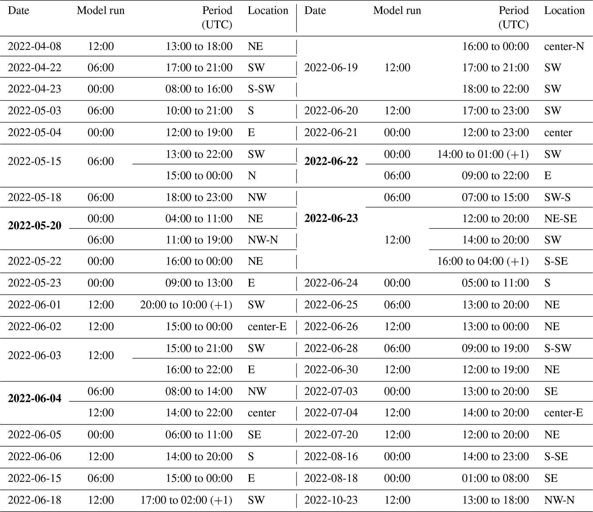
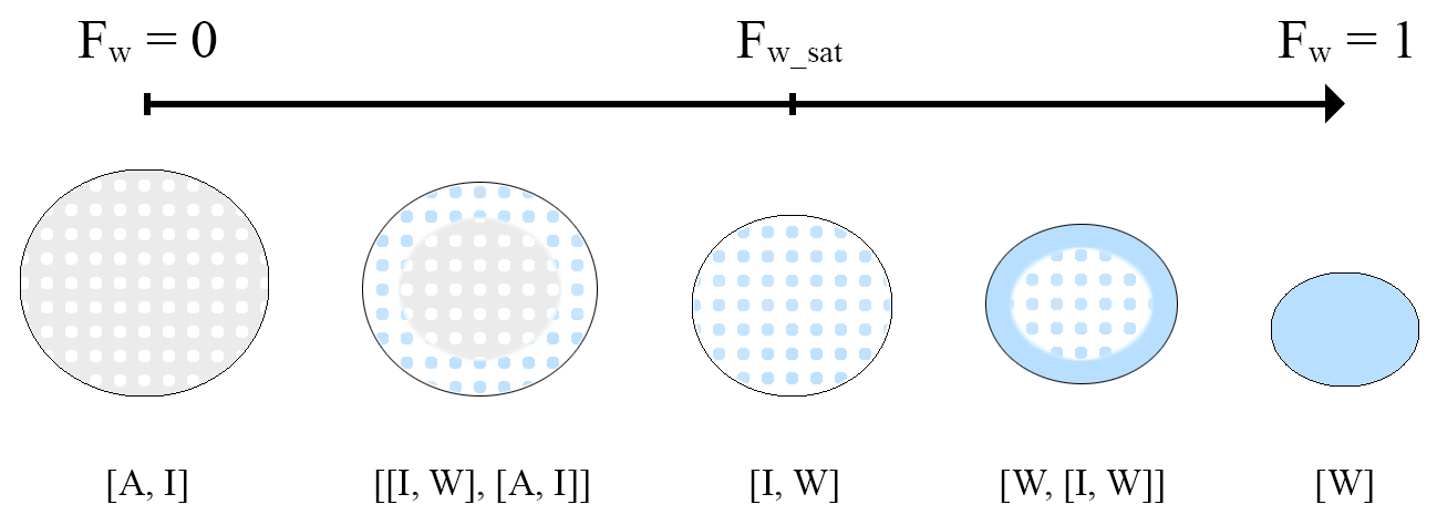
Figure B1Illustration of the graupel melting process as a function of the liquid water fraction Fw, with a matrix/inclusion approach. Air (A), ice (I), and liquid water (W) are respectively shown in gray, white, and blue. The various combinations [matrix, inclusions] used to calculate the dielectric constant according to the Maxwell-Garnett approximation (see Sect. 2.4) are also shown. Taken with permission from Fig. 4.1 of Le Bastard (2019).
As previously described in Sect. 2.4, nonhomogeneous hydrometeors are assimilated to matrices in which inclusions are inserted. The melting process can be divided into five steps (as shown by Fig. B1) based on the estimated liquid water fraction Fw of the particle.
-
Initial state: Fw = 0; the dry graupel is considered to be an ice particle with inclusions of air.
-
Step 1: 0 < Fw < ; the graupel starts melting, with the melted water first soaking the air cavities from the outside to the inside. This outer layer plays the role of a matrix for the whole particle, while the core (still an air matrix with ice inclusions) plays the role of an inclusion. The melting outer layer is considered to be a matrix of ice with inclusions of water.
-
Step 2: Fw = ; all air cavities are filled by melted water.
-
Step 3: < Fw < 1; the particle starts forming an outer water shell, while the core is composed of pure ice and water only. The particle is considered to be a matrix of water with inclusions of ice.
-
Final state: Fw = 1; the whole graupel is melted.
Therefore, the estimation of the equivalent diameter Deq that is needed to retrieve the scattering coefficients, as well as the dielectric constant, is tailored to the two stages of the melting process.
B1 Equivalent diameter of melting graupel
We want to remind the reader that the only pieces of information accessible by the forward operator are the variables related to the dry species. Thus, will refer to the initial graupel density, which is the density of the dry graupel provided by the model. implicitly includes the contribution of air, which means that (with ρi being the density of pure ice) if there are air cavities inside the particle.
B1.1
To compute the scattering coefficients of the melting graupel, a spherical melted equivalent diameter is first estimated. The wet graupel volume Vwg is equal to the volume of a sphere of equivalent diameter Deq.
As the graupel melts, Vwg can be expressed as a function of the initial volume of the dry graupel (of equivalent spherical diameter D) and the volume of melted graupel Vmg.
By conservation of mass, the mass of melted graupel mmg is equal to the mass of water created mw.
Also, the water fraction can be defined as the mass of water out of the total mass of the wet graupel. In this operator, , and thus, the mass of water created is
By combining Eqs. (B1), (B2), (B3), and (B4), the equivalent diameter Deq for can finally be expressed as
B1.2 Estimation of
Saturation is reached when the air cavities are fully soaked by water. The volume of the cavities Vc depends on the liquid water fraction Fw. In other words, when Vc = 0.
First, we need to determine the initial volume of the cavities when the particle is dry (at Fw=0), i.e., only made of air and ice.
Then, when the graupel starts melting, the new volume of air cavities can be expressed as
Vi can be deduced by the conservation of the mass.
The expression of Vw comes directly from Eq. (B4).
By replacing Vi and Vw in Eq. (B7),
Finally, the volume of the air cavities for a liquid water fraction comprised between 0 and is the initially available volume from which the new volume occupied is subtracted.
As previously stated, saturation () is reached for Vc = 0. Thus, with Eq. (B12) it finally comes that
B1.3
Once fully soaked, the particle starts building a water shell. At this stage, the graupel is composed of pure ice and water only. The volume of the wet graupel is thus
Its mass mwg can be expressed as a function of the mass of ice and the mass of water, including the water within the core and in the shell, by conservation of mass using Eq. (B4).
By expressing mi as a function of mg, Eq. (B14) can be written as
Finally, with Eqs. (B1) and (B16), the equivalent diameter for is
B2 Dielectric constant computation
The Maxwell Garnett (1904) formulation can be used to define the permittivity of the mixed phase particles, as long as the inclusions are spherical and remain small compared with the wavelength. Let ϵmat be the matrix permittivity and ϵinc the permittivity of inclusions. Following Maxwell Garnett (1904) and Wolfensberger and Berne (2018), the permittivity of nonhomogeneous hydrometeors can be expressed as
Based on Fig. B1, the effective permittivity can be expressed as
with the volume fractions involved in the calculation being
B3 PSD for melting hydrometeors
As the liquid water fraction increases, the particle size distribution gradually changes from that of iced particles to that of rain. The flux-based approach used here comes from Szyrmer and Zawadzki (1999). Given the hypothesis of no aggregation of the snowflakes and no breakup of the raindrops, at a stationary state, one iced particle leads to one raindrop as the particle melts. Thus, it can be stated that the flow of particles is conserved (subscripts wp and p stand for “wet particle” and “dry particle”, respectively):
with N being the number concentration and v the terminal velocity of the corresponding hydrometeors. The terminal velocities of wet particles are computed from a combination of the terminal velocities of rain vr and dry particles vp, following Wolfensberger and Berne (2018).
Then, knowing Fw for each Deq, the total wet particle number concentration Nwp can be expressed.
This section is only intended to provide a general overview of the theoretical polarimetric values that the A16 forward operator can reach for the range of contents and concentrations observed in this study. Values of ZH, ZDR, and KDP are presented herein as a function of the content for different hydrometeor classes and for a one-moment (Fig. C1) or two-moment PSD (Figs. C2, C3). Please note that we have compared ICE3 one-moment microphysics to LIMA microphysics, the latter being two-moment only for rain and ice.
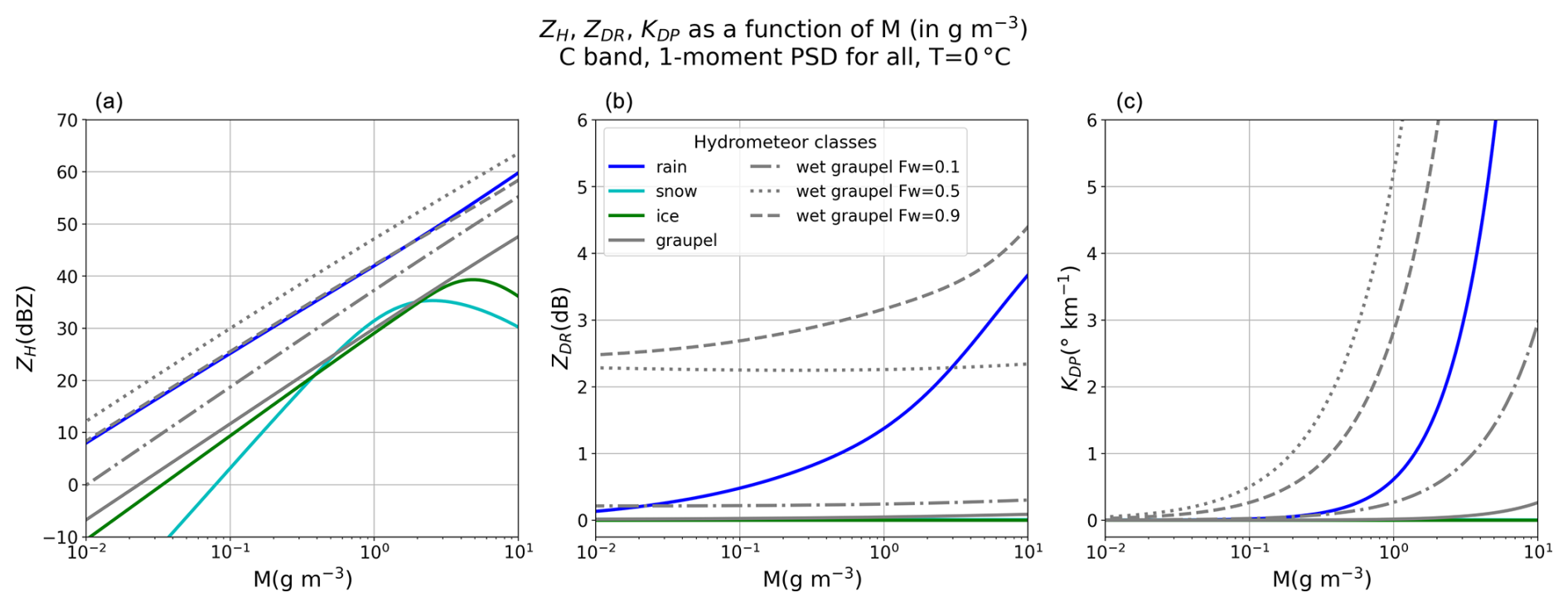
Figure C1Theoretical polarimetric outputs of the A16 forward operator for one-moment hydrometeor species. From left to right: reflectivity, differential reflectivity, and specific differential phase as a function of the content. Values for different liquid water fractions of the wet graupel have been added to emphasize the impact of graupel wetness on polarimetric values in the A16 operator.
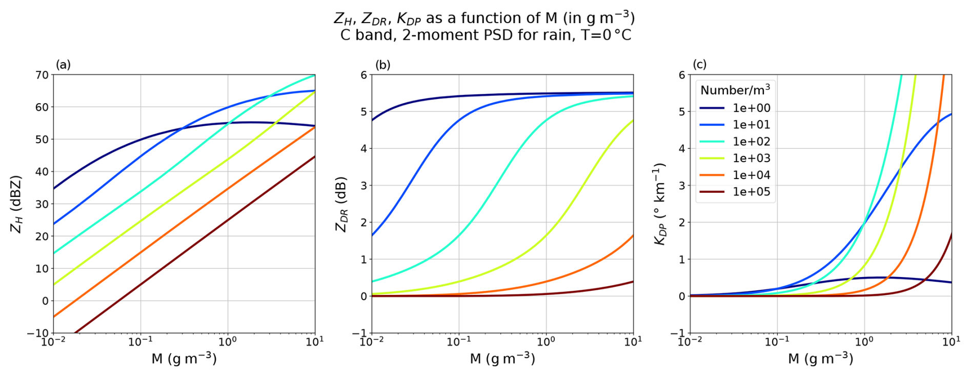
Figure C2Theoretical polarimetric outputs of the A16 forward operator for a two-moment rain hydrometeor class and for different number concentrations. From left to right: reflectivity, differential reflectivity, and specific differential phase as a function of the content.
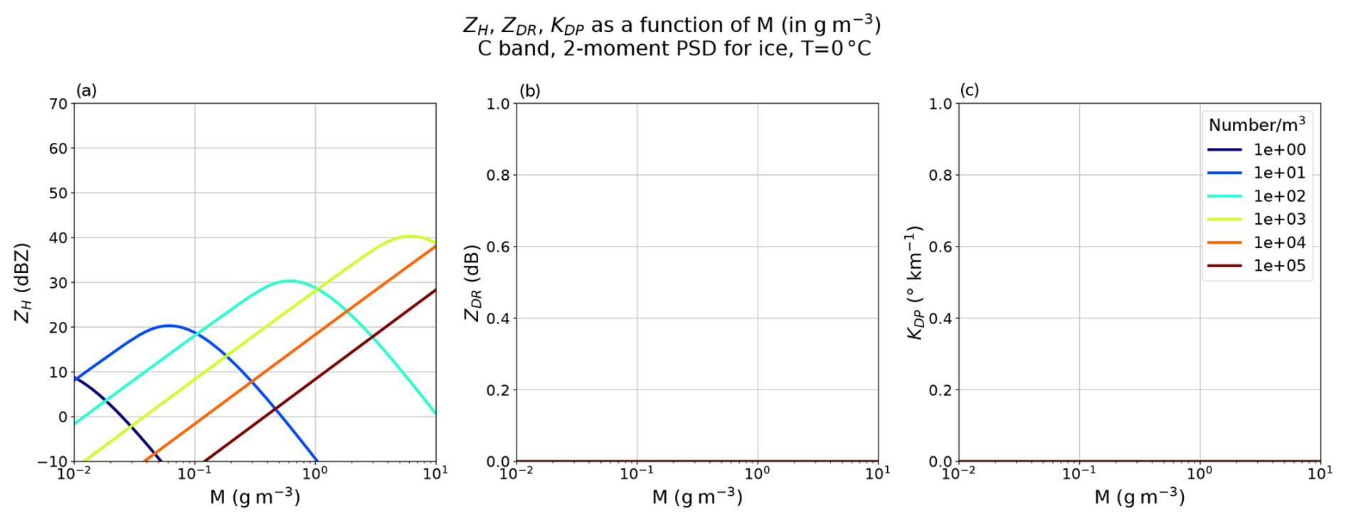
Figure C3Theoretical polarimetric outputs of the A16 forward operator for a two-moment ice hydrometeor class and for different number concentrations. From left to right: reflectivity, differential reflectivity, and specific differential phase as a function of the content.
Table D1Settings of the open-source Python package tobac, used in the tracking step, for cell envelope, cell core, and ZDR columns objects.
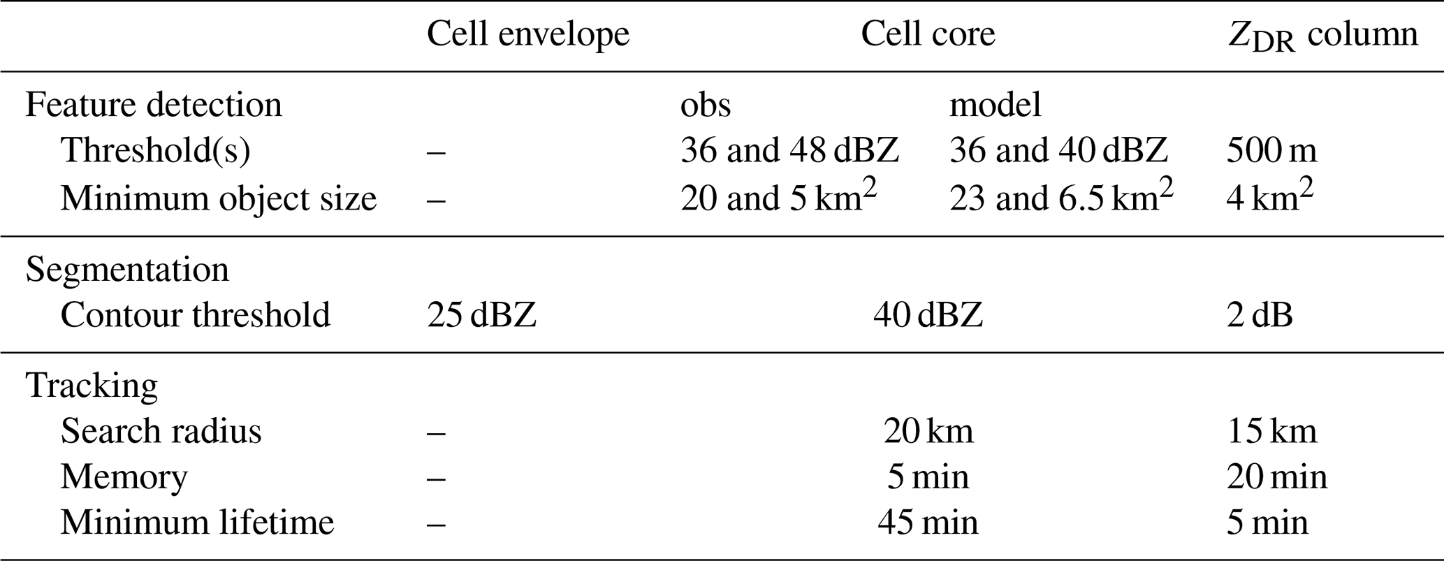
The radar forward operator software is publicly available at https://github.com/UMR-CNRM/operadar (Augros, 2025). This software is governed by the open-source CeCILL-C license.
The raw volumetric dual-polarization radar data are publicly accessible through the AERIS platform (https://radarsmf.aeris-data.fr/description/?uuid=dea49d60-1489-458e-a8de-589d21b14ca4, Météo-France, 2024) under a research and development license. The lookup tables used to simulate synthetic radar data from the model outputs are available at https://www.easydata.earth/metadataRecord/cbfad634-d22e-4013-862c-c79b57e147ca (last access: 6 August 2025, under CC-BY-4.0; https://doi.org/10.57932/8658B5E3-8314-476B-B3DF-29958AF6D9D6, David, 2025a; https://doi.org/10.57932/D321C87D-053F-494E-A5F9-C638D6F34E4A, David, 2025b; https://doi.org/10.57932/62183D3A-22D3-42CD-B7BF-CCFA037696D1, David, 2025c; https://doi.org/10.57932/BE018834-ACDD-48DA-86F0-9CA57908DE6C, David, 2025d). The model data that support the findings of this study are available from the corresponding author upon request.
A demonstration of the tracking performed on the 2022-06-20 thunderstorm event is available at https://doi.org/10.57932/346805fe-faf3-4c86-96b7-956e1735f495 (David, 2025e).
CD designed the methodology, developed the ZDR column algorithm, realized the analysis, and wrote the paper. CA, BV, and FB helped in the conceptualization, methodology, and supervision of the paper. TLB implemented the operator's melting scheme and contributed to its description in Appendix B.
The contact author has declared that none of the authors has any competing interests.
Publisher's note: Copernicus Publications remains neutral with regard to jurisdictional claims made in the text, published maps, institutional affiliations, or any other geographical representation in this paper. While Copernicus Publications makes every effort to include appropriate place names, the final responsibility lies with the authors.
This study has been partially supported through the grant EUR TESS no. ANR-18-EURE-0018 in the framework of the Programme des Investissements d'Avenir. The authors would like to thank Alexander Ryzhkov, Jacob Carlin, and Jeffrey Snyder for the discussions and constructive feedback that helped us better understand our limitations and pave the way for future prospects. The authors would also like to express their gratitude to John Krause for his review of the paper, which enhanced its overall quality.
This research has been supported by the Agence Nationale de la Recherche (EUR TESS, grant no. ANR-18-EURE-0018).
This paper was edited by Gianfranco Vulpiani and reviewed by two anonymous referees.
Al-Sakka, H., Boumahmoud, A.-A., Fradon, B., Frasier, S. J., and Tabary, P.: A New Fuzzy Logic Hydrometeor Classification Scheme Applied to the French X-, C-, and S-Band Polarimetric Radars, J. Appl. Meteorol. Clim., 52, 2328–2344, https://doi.org/10.1175/JAMC-D-12-0236.1, 2013. a, b
Aregger, M., Martius, O., Germann, U., and Hering, A.: Differential reflectivity columns and hail: linking C-band radar-based estimated column characteristics to crowdsourced hail observations in Switzerland, arXiv [preprint], https://doi.org/10.48550/arXiv.2410.10499, 14 October 2024. a
Augros, C.: OPERADAR (Version 0.0), CNRM, Météo-France, GitHub [code], https://github.com/UMR-CNRM/operadar, 2025. a
Augros, C., Caumont, O., Ducrocq, V., Gaussiat, N., and Tabary, P.: Comparisons between S-, C- and X-band polarimetric radar observations and convective-scale simulations of the HyMeX first special observing period, Q. J. Royal Meteorological Soc., 142, 347–362, https://doi.org/10.1002/qj.2572, 2016. a, b, c, d
Augros, C., Caumont, O., Ducrocq, V., and Gaussiat, N.: Assimilation of radar dual-polarization observations in the AROME model, Q. J. Roy. Meteor. Soc., 144, 1352–1368, https://doi.org/10.1002/qj.3269, 2018. a
Barnes, S. L.: A Technique for Maximizing Details in Numerical Weather Map Analysis, J. Appl. Meteorol. Clim., 3, 396–409, https://doi.org/10.1175/1520-0450(1964)003<0396:ATFMDI>2.0.CO;2, 1964. a
Besic, N., Figueras i Ventura, J., Grazioli, J., Gabella, M., Germann, U., and Berne, A.: Hydrometeor classification through statistical clustering of polarimetric radar measurements: a semi-supervised approach, Atmos. Meas. Tech., 9, 4425–4445, https://doi.org/10.5194/amt-9-4425-2016, 2016. a
Brandes, E. A., Ikeda, K., Zhang, G., Schönhuber, M., and Rasmussen, R. M.: A Statistical and Physical Description of Hydrometeor Distributions in Colorado Snowstorms Using a Video Disdrometer, J. Appl. Meteorol. Clim., 46, 634–650, https://doi.org/10.1175/JAM2489.1, 2007. a
Brousseau, P., Seity, Y., Ricard, D., and Léger, J.: Improvement of the forecast of convective activity from the AROME-France system, Q. J. Roy. Meteor. Soc., 142, 2231–2243, https://doi.org/10.1002/qj.2822, 2016. a, b, c, d, e
Bénard, P., Vivoda, J., Mašek, J., Smolíková, P., Yessad, K., Smith, C., Brožková, R., and Geleyn, J.-F.: Dynamical kernel of the Aladin–NH spectral limited-area model: Revised formulation and sensitivity experiments, Q. J. Roy. Meteor. Soc., 136, 155–169, https://doi.org/10.1002/qj.522, 2010. a
Cai, H. and Dumais, R. E.: Object-Based Evaluation of a Numerical Weather Prediction Model's Performance through Forecast Storm Characteristic Analysis, Weather Forecast., 30, 1451–1468, https://doi.org/10.1175/WAF-D-15-0008.1, 2015. a
Carlin, J. T. and Ryzhkov, A. V.: Estimation of Melting-Layer Cooling Rate from Dual-Polarization Radar: Spectral Bin Model Simulations, J. Appl. Meteorol. Clim., 58, 1485–1508, https://doi.org/10.1175/JAMC-D-18-0343.1, 2019. a
Carlin, J. T., Gao, J., Snyder, J. C., and Ryzhkov, A. V.: Assimilation of ZDR Columns for Improving the Spinup and Forecast of Convective Storms in Storm-Scale Models: Proof-of-Concept Experiments, Mon. Weather Rev., 145, 5033–5057, https://doi.org/10.1175/MWR-D-17-0103.1, 2017. a, b, c
Carpenter, A. E., Jones, T. R., Lamprecht, M. R., Clarke, C., Kang, I. H., Friman, O., Guertin, D. A., Chang, J. H., Lindquist, R. A., Moffat, J., Golland, P., and Sabatini, D. M.: CellProfiler: image analysis software for identifying and quantifying cell phenotypes, Genome Biol., 7, R100, https://doi.org/10.1186/gb-2006-7-10-r100, 2006. a
Caumont, O., Ducrocq, V., Delrieu, G., Gosset, M., Pinty, J.-P., Parent du Châtelet, J., Andrieu, H., Lemaître, Y., and Scialom, G.: A Radar Simulator for High-Resolution Nonhydrostatic Models, J. Atmos. Ocean. Tech., 23, 1049–1067, https://doi.org/10.1175/JTECH1905.1, 2006. a
Caumont, O., Ducrocq, V., Wattrelot, E., Jaubert, G., and Pradier-Vabre, S.: 1D+3DVar assimilation of radar reflectivity data: a proof of concept, Tellus A, 62, 173–187, https://doi.org/10.1111/j.1600-0870.2009.00430.x, 2010. a
Caumont, O., Mandement, M., Bouttier, F., Eeckman, J., Lebeaupin Brossier, C., Lovat, A., Nuissier, O., and Laurantin, O.: The heavy precipitation event of 14–15 October 2018 in the Aude catchment: a meteorological study based on operational numerical weather prediction systems and standard and personal observations, Nat. Hazards Earth Syst. Sci., 21, 1135–1157, https://doi.org/10.5194/nhess-21-1135-2021, 2021. a
Caylor, I. J. and Illingworth, A. J.: Radar Observations and Modelling of Warm Rain Initiation, Q. J. Roy. Meteor. Soc., 113, 1171–1191, https://doi.org/10.1002/qj.49711347806, 1987. a
Champeaux, J.-L., Laurantin, O., Mercier, B., Mounier, F., Lassegues, P., and Tabary, P.: Quantitative precipitation estimations using rain gauges and radar networks: inventory and prospects at Meteo-France, in: WMO Joint Meeting of CGS Expert Team on Surface-based Remotely-sensed Observations and CIMO Expert Team on Operational Remote Sensing, 5, 1–11, 2011. a
Cohard, J.-M., Pinty, J.-P., and Bedos, C.: Extending Twomey’s Analytical Estimate of Nucleated Cloud Droplet Concentrations from CCN Spectra, J. Atmos. Sci., 55, 3348–3357, https://doi.org/10.1175/1520-0469(1998)055<3348:ETSAEO>2.0.CO;2, 1998. a
Courtier, P., Freydier, C., Geleyn, J., Rabier, F., and Rochas, M.: The ARPEGE project at Météo‐France, in: Seminar on Numerical Methods on Atmospheric Models, ECMWF, Reading, UK, 193–231, https://www.ecmwf.int/sites/default/files/elibrary/1991/8798-arpege-project-meteo-france.pdf (last access: 28 May 2024), 1991. a
Courtier, P., Thépaut, J.-N., and Hollingsworth, A.: A strategy for operational implementation of 4D-Var, using an incremental approach, Q. J. Roy. Meteor. Soc., 120, 1367–1387, https://doi.org/10.1002/qj.49712051912, 1994. a
Cuxart, J., Bougeault, P., and Redelsperger, J.-L.: A turbulence scheme allowing for mesoscale and large-eddy simulations, Q. J. Roy. Meteor. Soc., 126, 1–30, https://doi.org/10.1002/qj.49712656202, 2000. a
David, C.: C-band tables with ICE3 microphysics for OPERADAR, EaSy Data [data set], https://doi.org/10.57932/8658B5E3-8314-476B-B3DF-29958AF6D9D6, 2025a. a
David, C.: C-band tables with LIMA microphysics for OPERADAR, EaSy Data [data set], https://doi.org/10.57932/D321C87D-053F-494E-A5F9-C638D6F34E4A, 2025b. a
David, C.: S-band tables with ICE3 microphysics for OPERADAR, EaSy Data [data set], https://doi.org/10.57932/62183D3A-22D3-42CD-B7BF-CCFA037696D1, 2025c. a
David, C.: S-band tables with LIMA microphysics fo OPERADAR, EaSy Data [data set], https://doi.org/10.57932/BE018834-ACDD-48DA-86F0-9CA57908DE6C, 2025d. a
David, C.: 2022-06-20 radar and model data cell tracking, EaSy Data [video], https://doi.org/10.57932/346805fe-faf3-4c86-96b7-956e1735f495, 2025e. a, b
Davis, C., Brown, B., and Bullock, R.: Object-Based Verification of Precipitation Forecasts. Part I: Methodology and Application to Mesoscale Rain Areas, Mon. Weather Rev., 134, 1772–1784, https://doi.org/10.1175/MWR3145.1, 2006. a
Davis, C. A., Brown, B. G., Bullock, R., and Halley-Gotway, J.: The Method for Object-Based Diagnostic Evaluation (MODE) Applied to Numerical Forecasts from the 2005 NSSL/SPC Spring Program, Weather Forecast., 24, 1252–1267, https://doi.org/10.1175/2009WAF2222241.1, 2009. a
Dawson, D. T., Mansell, E. R., Jung, Y., Wicker, L. J., Kumjian, M. R., and Xue, M.: Low-Level ZDR Signatures in Supercell Forward Flanks: The Role of Size Sorting and Melting of Hail, J. Atmos. Sci., 71, 276–299, https://doi.org/10.1175/JAS-D-13-0118.1, 2014. a, b
Donaldson, R. J., Dyer, R. M., and Kraus, M. J.: An Objective Evaluator of Techniques for Predicting Severe Weather Events, Tech. Rep. ADA015773, Air Force Cambridge Research Labs Hanscom AFB Mass, https://ntrl.ntis.gov/NTRL/dashboard/searchResults/titleDetail/ADA015773.xhtml (last access: 20 May 2024), 1975. a
Dotzek, N., Groenemeijer, P., Feuerstein, B., and Holzer, A.: Overview of ESSL's severe convective storms research using the European Severe Weather Database ESWD, Atmos. Res., 93, 575–586, https://doi.org/10.1016/j.atmosres.2008.10.020, 2009. a, b
Draine, B. T.: The Discrete-Dipole Approximation and Its Application to Interstellar Graphite Grains, Astrophys. J., 333, 848, https://doi.org/10.1086/166795, 1988. a
Ducongé, L., Lac, C., Vié, B., Bergot, T., and Price, J. D.: Fog in heterogeneous environments: the relative importance of local and non-local processes on radiative-advective fog formation, Q. J. Roy. Meteor. Soc., 146, 2522–2546, https://doi.org/10.1002/qj.3783, 2020. a
Figueras i Ventura, J., Boumahmoud, A.-A., Fradon, B., Dupuy, P., and Tabary, P.: Long-term monitoring of French polarimetric radar data quality and evaluation of several polarimetric quantitative precipitation estimators in ideal conditions for operational implementation at C-band, Q. J. Roy. Meteor. Soc., 138, 2212–2228, https://doi.org/10.1002/qj.1934, 2012. a
Forcadell, V., Augros, C., Caumont, O., Dedieu, K., Ouradou, M., David, C., Figueras i Ventura, J., Laurantin, O., and Al-Sakka, H.: Severe-hail detection with C-band dual-polarisation radars using convolutional neural networks, Atmos. Meas. Tech., 17, 6707–6734, https://doi.org/10.5194/amt-17-6707-2024, 2024. a
Fouquart, Y. and Bonnel, B.: Computations of solar heating of the Earth's atmosphere: A new parameterization, Beiträge zur Physik der Atmosphäre, 53, 35–62, https://cir.nii.ac.jp/crid/1370017282189594910 (last access: 5 June 2024), 1980. a
Gallus Jr., W. A. and Pfeifer, M.: Intercomparison of simulations using 5 WRF microphysical schemes with dual-Polarization data for a German squall line, Adv. Geosci., 16, 109–116, https://doi.org/10.5194/adgeo-16-109-2008, 2008. a
Gasper, F., Goergen, K., Shrestha, P., Sulis, M., Rihani, J., Geimer, M., and Kollet, S.: Implementation and scaling of the fully coupled Terrestrial Systems Modeling Platform (TerrSysMP v1.0) in a massively parallel supercomputing environment – a case study on JUQUEEN (IBM Blue Gene/Q), Geosci. Model Dev., 7, 2531–2543, https://doi.org/10.5194/gmd-7-2531-2014, 2014. a
Gourley, J. J., Tabary, P., and Parent du Chatelet, J.: A Fuzzy Logic Algorithm for the Separation of Precipitating from Nonprecipitating Echoes Using Polarimetric Radar Observations, J. Atmos. Ocean. Tech., 24, 1439–1451, https://doi.org/10.1175/JTECH2035.1, 2007. a
Hall, M. P. M., Goddard, J. W. F., and Cherry, S. M.: Identification of hydrometeors and other targets by dual-polarization radar, Radio Sci., 19, 132–140, https://doi.org/10.1029/RS019i001p00132, 1984. a
Heidke, P.: Berechnung Des Erfolges Und Der Güte Der Windstärkevorhersagen Im Sturmwarnungsdienst (Calculation of the success and the goodness of strong wind forecasts in the storm warning service), Geografiska Annaler, 8, 301–349, https://doi.org/10.1080/20014422.1926.11881138, 1926. a
Heikenfeld, M., Marinescu, P. J., Christensen, M., Watson-Parris, D., Senf, F., van den Heever, S. C., and Stier, P.: tobac 1.2: towards a flexible framework for tracking and analysis of clouds in diverse datasets, Geosci. Model Dev., 12, 4551–4570, https://doi.org/10.5194/gmd-12-4551-2019, 2019. a, b, c, d, e
Helmus, J. J. and Collis, S. M.: The Python ARM Radar Toolkit (Py-ART), a Library for Working with Weather Radar Data in the Python Programming Language, Journal of Open Research Software, 4, e25, https://doi.org/10.5334/jors.119, 2016. a
Hong, S.-Y. and Lim, J.-O. J.: The WRF Single-Moment 6-Class Microphysics Scheme (WSM6), J. Korean Meteor. Soc., 42, 129–151, 2006. a
Houze Jr., R. A.: Cloud Dynamics, Academic Press, ISBN 978-0-08-092146-4, 2014. a
Höller, H., Hagen, M., Meischner, P. F., Bringi, V. N., and Hubbert, J.: Life Cycle and Precipitation Formation in a Hybrid-Type Hailstorm Revealed by Polarimetric and Doppler Radar Measurements, J. Atmos. Sci., 51, 2500–2522, https://doi.org/10.1175/1520-0469(1994)051<2500:LCAPFI>2.0.CO;2, 1994. a
Hubbert, J. C., Ellis, S. M., Chang, W.-Y., Rutledge, S., and Dixon, M.: odeling and Interpretation of S-Band Ice Crystal Depolarization Signatures from Data Obtained by Simultaneously Transmitting Horizontally and Vertically Polarized Fields, J. Appl. Meteorol. Clim., 53, 1659–1677, https://doi.org/10.1175/JAMC-D-13-0158.1, 2014. a
Jameson, A. R.: Microphysical Interpretation of Multiparameter Radar Measurements in Rain. Part III: Interpretation and Measurement of Propagation Differential Phase Shift between Orthogonal Linear Polarizations, J. Atmos. Sci., 42, 607–614, https://doi.org/10.1175/1520-0469(1985)042<0607:MIOMRM>2.0.CO;2, 1985. a
Johnson, M., Jung, Y., Dawson, D. T., and Xue, M.: Comparison of Simulated Polarimetric Signatures in Idealized Supercell Storms Using Two-Moment Bulk Microphysics Schemes in WRF, Mon. Weather Rev., 144, 971–996, https://doi.org/10.1175/MWR-D-15-0233.1, 2016. a, b
Jung, Y., Zhang, G., and Xue, M.: Assimilation of Simulated Polarimetric Radar Data for a Convective Storm Using the Ensemble Kalman Filter. Part I: Observation Operators for Reflectivity and Polarimetric Variables, Mon. Weather Rev., 136, 2228–2245, https://doi.org/10.1175/2007MWR2083.1, 2008. a
Jung, Y., Xue, M., and Zhang, G.: Simulations of Polarimetric Radar Signatures of a Supercell Storm Using a Two-Moment Bulk Microphysics Scheme, J. Appl. Meteorol. Clim., 49, 146–163, https://doi.org/10.1175/2009JAMC2178.1, 2010. a
Kennedy, P. C. and Rutledge, S. A.: Dual-Doppler and Multiparameter Radar Observations of a Bow-Echo Hailstorm, Mon. Weather Rev., 123, 921–943, https://doi.org/10.1175/1520-0493(1995)123<0921:DDAMRO>2.0.CO;2, 1995. a
Kennedy, P. C., Rutledge, S. A., Petersen, W. A., and Bringi, V. N.: Polarimetric Radar Observations of Hail Formation, J. Appl. Meteorol. Clim., 40, 1347–1366, https://doi.org/10.1175/1520-0450(2001)040<1347:PROOHF>2.0.CO;2, 2001. a
Kessler, E.: On the Distribution and Continuity of Water Substance in Atmosphere Circulations, American Meteorological Society, Boston, MA, 10, 1–84, https://doi.org/10.1007/978-1-935704-36-2, 1969. a
Krause, J. and Klaus, V.: Identifying ZDR Columns in Radar Data with the Hotspot Technique, Weather Forecast., 39, 581–595, https://doi.org/10.1175/WAF-D-23-0146.1, 2024. a, b
Kumjian, M.: Principles and applications of dual-polarization weather radar. Part II: Warm- and cold-season applications, Journal of Operational Meteorology, 1, 243–264, https://doi.org/10.15191/nwajom.2013.0120, 2013. a
Kumjian, M. R. and Ryzhkov, A. V.: Polarimetric Signatures in Supercell Thunderstorms, J. Appl. Meteorol. Clim., 47, 1940–1961, https://doi.org/10.1175/2007JAMC1874.1, 2008. a, b
Kumjian, M. R., Ganson, S. M., and Ryzhkov, A. V.: Freezing of Raindrops in Deep Convective Updrafts: A Microphysical and Polarimetric Model, J. Atmos. Sci., 69, 3471–3490, https://doi.org/10.1175/JAS-D-12-067.1, 2012. a
Kumjian, M. R., Khain, A. P., Benmoshe, N., Ilotoviz, E., Ryzhkov, A. V., and Phillips, V. T. J.: The Anatomy and Physics of ZDR Columns: Investigating a Polarimetric Radar Signature with a Spectral Bin Microphysical Model, J. Appl. Meteorol. Clim., 53, 1820–1843, https://doi.org/10.1175/JAMC-D-13-0354.1, 2014. a
Kumjian, M. R., Lombardo, K., and Loeffler, S.: The Evolution of Hail Production in Simulated Supercell Storms, J. Atmos. Sciences, 78, 3417–3440, https://doi.org/10.1175/JAS-D-21-0034.1, 2021. a, b, c, d
Kuster, C. M., Snyder, J. C., Schuur, T. J., Lindley, T. T., Heinselman, P. L., Furtado, J. C., Brogden, J. W., and Toomey, R.: Rapid-Update Radar Observations of ZDR Column Depth and Its Use in the Warning Decision Process, Weather Forecast., 34, 1173–1188, https://doi.org/10.1175/WAF-D-19-0024.1, 2019. a, b, c, d
Kuster, C. M., Schuur, T. J., Lindley, T. T., and Snyder, J. C.: Using ZDR Columns in Forecaster Conceptual Models and Warning Decision-Making, Weather Forecast., 35, 2507–2522, https://doi.org/10.1175/WAF-D-20-0083.1, 2020. a, b
Köcher, G., Zinner, T., Knote, C., Tetoni, E., Ewald, F., and Hagen, M.: Evaluation of convective cloud microphysics in numerical weather prediction models with dual-wavelength polarimetric radar observations: methods and examples, Atmos. Meas. Tech., 15, 1033–1054, https://doi.org/10.5194/amt-15-1033-2022, 2022. a, b, c, d, e, f
Köcher, G., Zinner, T., and Knote, C.: Influence of cloud microphysics schemes on weather model predictions of heavy precipitation, Atmos. Chem. Phys., 23, 6255–6269, https://doi.org/10.5194/acp-23-6255-2023, 2023. a
ac, C., Chaboureau, J.-P., Masson, V., Pinty, J.-P., Tulet, P., Escobar, J., Leriche, M., Barthe, C., Aouizerats, B., Augros, C., Aumond, P., Auguste, F., Bechtold, P., Berthet, S., Bielli, S., Bosseur, F., Caumont, O., Cohard, J.-M., Colin, J., Couvreux, F., Cuxart, J., Delautier, G., Dauhut, T., Ducrocq, V., Filippi, J.-B., Gazen, D., Geoffroy, O., Gheusi, F., Honnert, R., Lafore, J.-P., Lebeaupin Brossier, C., Libois, Q., Lunet, T., Mari, C., Maric, T., Mascart, P., Mogé, M., Molinié, G., Nuissier, O., Pantillon, F., Peyrillé, P., Pergaud, J., Perraud, E., Pianezze, J., Redelsperger, J.-L., Ricard, D., Richard, E., Riette, S., Rodier, Q., Schoetter, R., Seyfried, L., Stein, J., Suhre, K., Taufour, M., Thouron, O., Turner, S., Verrelle, A., Vié, B., Visentin, F., Vionnet, V., and Wautelet, P.: Overview of the Meso-NH model version 5.4 and its applications, Geosci. Model Dev., 11, 1929–1969, https://doi.org/10.5194/gmd-11-1929-2018, 2018. a, b
Le Bastard, T.: Utilisation des données radar volumiques et d'un modèle de PNT à haute résolution pour une meilleure estimation quantitative des précipitations en plaine et sur les massifs montagneux, These de doctorat, Toulouse, INPT, https://theses.fr/2019INPT0140 (last access: 17 May 2025), 2019 (in French with English abstract). a
Li, X., Mecikalski, J. R., and Posselt, D.: An Ice-Phase Microphysics Forward Model and Preliminary Results of Polarimetric Radar Data Assimilation, Mon. Weather Rev., 145, 683–708, https://doi.org/10.1175/MWR-D-16-0035.1, 2017. a
Liu, P., Zhang, G., Carlin, J. T., and Gao, J.: A New Melting Model and Its Implementation in Parameterized Forward Operators for Polarimetric Radar Data Simulation With Double Moment Microphysics Schemes, J. Geophys. Res.-Atmos., 129, e2023JD040026, https://doi.org/10.1029/2023JD040026, 2024. a
Lo, C. H. B., Stein, T. H. M., Scovell, R. W., Westbrook, C. D., Darlington, T., and Lean, H. W.: Use of ZDR columns for early detection of severe convection within the operational radar network of the United Kingdom, Meteorol. Appl., 31, e2159, https://doi.org/10.1002/met.2159, 2024. a
Masson, V., Le Moigne, P., Martin, E., Faroux, S., Alias, A., Alkama, R., Belamari, S., Barbu, A., Boone, A., Bouyssel, F., Brousseau, P., Brun, E., Calvet, J.-C., Carrer, D., Decharme, B., Delire, C., Donier, S., Essaouini, K., Gibelin, A.-L., Giordani, H., Habets, F., Jidane, M., Kerdraon, G., Kourzeneva, E., Lafaysse, M., Lafont, S., Lebeaupin Brossier, C., Lemonsu, A., Mahfouf, J.-F., Marguinaud, P., Mokhtari, M., Morin, S., Pigeon, G., Salgado, R., Seity, Y., Taillefer, F., Tanguy, G., Tulet, P., Vincendon, B., Vionnet, V., and Voldoire, A.: The SURFEXv7.2 land and ocean surface platform for coupled or offline simulation of earth surface variables and fluxes, Geosci. Model Dev., 6, 929–960, https://doi.org/10.5194/gmd-6-929-2013, 2013. a
Matrosov, S. Y., Reinking, R. F., Kropfli, R. A., and Bartram, B. W.: Estimation of Ice Hydrometeor Types and Shapes from Radar Polarization Measurements, J. Atmos. Ocean. Tech., 13, 85–96, https://doi.org/10.1175/1520-0426(1996)013<0085:EOIHTA>2.0.CO;2, 1996. a
Maxwell Garnett, J. C.: Colours in metal glasses and in metallic films, Philos. T. R. Soc. Lond., 203, 385–420, https://doi.org/10.1098/rsta.1904.0024, 1904. a, b
Meischner, P., Guzzi, R., Imboden, D., Lanzerotti, L. J., and Platt, U. (Eds.): Weather Radar, Physics of Earth and Space Environments, Springer, Berlin, Heidelberg, https://doi.org/10.1007/978-3-662-05202-0, ISBN 978-3-642-05561-4, 978-3-662-05202-0, 2004. a
Météo-France: RADAR double-polar radial raw data from PAM* products, AERIS [data set], https://radarsmf.aeris-data.fr/description/?uuid=dea49d60-1489-458e-a8de-589d21b14ca4 (last access: 6 August 2025), 2024. a
Meyers, M. P., DeMott, P. J., and Cotton, W. R.: New Primary Ice-Nucleation Parameterizations in an Explicit Cloud Model, J. Appl. Meteorol. Clim., 31, 708–721, https://doi.org/10.1175/1520-0450(1992)031<0708:NPINPI>2.0.CO;2, 1992. a
Mishchenko, M. I. and Travis, L. D.: T-matrix computations of light scattering by large spheroidal particles, Opt. Commun., 109, 16–21, https://doi.org/10.1016/0030-4018(94)90731-5, 1994. a
Mlawer, E. J., Taubman, S. J., Brown, P. D., Iacono, M. J., and Clough, S. A.: Radiative transfer for inhomogeneous atmospheres: RRTM, a validated correlated-k model for the longwave, J. Geophys. Res.-Atmos., 102, 16663–16682, https://doi.org/10.1029/97JD00237, 1997. a
Morcrette, J.-J. and Fouquart, Y.: The Overlapping of Cloud Layers in Shortwave Radiation Parameterizations, J. Atmos. Sci., 43, 321–328, https://doi.org/10.1175/1520-0469(1986)043<0321:TOOCLI>2.0.CO;2, 1986. a
Murphy, A. and Daan, H.: Forecast evaluation, in: Probability, Statistics, and Decision Making in the Atmospheric Sciences, Westview Press, Chap. 10, 379–437, ISBN 13:978-0-367-28433 (hbk), 1985. a
Noilhan, J. and Mahfouf, J. F.: The ISBA land surface parameterisation scheme, Global Planet. Change, 13, 145–159, https://doi.org/10.1016/0921-8181(95)00043-7, 1996. a
Noilhan, J. and Planton, S.: A Simple Parameterization of Land Surface Processes for Meteorological Models, Mon. Weather Rev., 117, 536–549, https://doi.org/10.1175/1520-0493(1989)117<0536:ASPOLS>2.0.CO;2, 1989. a
Park, H. S., Ryzhkov, A. V., Zrnić, D. S., and Kim, K.-E.: The Hydrometeor Classification Algorithm for the Polarimetric WSR-88D: Description and Application to an MCS, Weather Forecast., 24, 730–748, https://doi.org/10.1175/2008WAF2222205.1, 2009. a, b
Pauley, P. M. and Wu, X.: The Theoretical, Discrete, and Actual Response of the Barnes Objective Analysis Scheme for One- and Two-Dimensional Fields, Mon. Weather Rev., 118, 1145–1164, https://doi.org/10.1175/1520-0493(1990)118<1145:TTDAAR>2.0.CO;2, 1990. a
Pergaud, J., Masson, V., Malardel, S., and Couvreux, F.: A Parameterization of Dry Thermals and Shallow Cumuli for Mesoscale Numerical Weather Prediction, Bound.-Lay. Meteorol., 132, 83–106, https://doi.org/10.1007/s10546-009-9388-0, 2009. a
Phillips, V. T. J., DeMott, P. J., and Andronache, C.: An Empirical Parameterization of Heterogeneous Ice Nucleation for Multiple Chemical Species of Aerosol, J. Atmos. Sci., 65, 2757–2783, https://doi.org/10.1175/2007JAS2546.1, 2008. a
Phillips, V. T. J., Demott, P. J., Andronache, C., Pratt, K. A., Prather, K. A., Subramanian, R., and Twohy, C.: Improvements to an Empirical Parameterization of Heterogeneous Ice Nucleation and Its Comparison with Observations, J. Atmos. Sci., 70, 378–409, https://doi.org/10.1175/JAS-D-12-080.1, 2013. a
Picca, J. and Ryzhkov, A.: A Dual-Wavelength Polarimetric Analysis of the 16 May 2010 Oklahoma City Extreme Hailstorm, Mon. Weather Rev., 140, 1385–1403, https://doi.org/10.1175/MWR-D-11-00112.1, 2012. a
Pinty, J.-P. and Jabouille, P.: A mixed-phase cloud parameterization for use in a mesoscale non-hydrostatic model: Simulations of a squall line of orographic precipitation, American Meteorological Society, Everett, WA, 217–220, http://195.83.22.22/mesonh/dir_publication/pinty_jabouille_ams_ccp1998.pdf (last access: 28 February 2025), 1998. a, b
Purcell, E. M. and Pennypacker, C. R.: Scattering and Absorption of Light by Nonspherical Dielectric Grains, Astrophysi. J., 186, 705–714, https://doi.org/10.1086/152538, 1973. a
Putnam, B., Xue, M., Jung, Y., Snook, N., and Zhang, G.: Ensemble Kalman Filter Assimilation of Polarimetric Radar Observations for the 20 May 2013 Oklahoma Tornadic Supercell Case, Mon. Weather Rev., 147, 2511–2533, https://doi.org/10.1175/MWR-D-18-0251.1, 2019. a
Putnam, B. J., Xue, M., Jung, Y., Zhang, G., and Kong, F.: Simulation of Polarimetric Radar Variables from 2013 CAPS Spring Experiment Storm-Scale Ensemble Forecasts and Evaluation of Microphysics Schemes, Mon. Weather Rev., 145, 49–73, https://doi.org/10.1175/MWR-D-15-0415.1, 2017. a, b, c
Rajeevan, M., Kesarkar, A., Thampi, S. B., Rao, T. N., Radhakrishna, B., and Rajasekhar, M.: Sensitivity of WRF cloud microphysics to simulations of a severe thunderstorm event over Southeast India, Ann. Geophys., 28, 603–619, https://doi.org/10.5194/angeo-28-603-2010, 2010. a
Rasmussen, R. M. and Heymsfield, A. J.: Melting and Shedding of Graupel and Hail. Part I: Model Physics, J. Atmos. Sci., 44, 2754–2763, https://doi.org/10.1175/1520-0469(1987)044<2754:MASOGA>2.0.CO;2, 1987. a, b
Reimann, L., Simmer, C., and Trömel, S.: Assimilation of 3D polarimetric microphysical retrievals in a convective-scale NWP system, Atmos. Chem. Phys., 23, 14219–14237, https://doi.org/10.5194/acp-23-14219-2023, 2023. a, b
Ricard, D., Lac, C., Riette, S., Legrand, R., and Mary, A.: Kinetic energy spectra characteristics of two convection-permitting limited-area models AROME and Meso-NH, Q. J. Roy. Meteor. Soc., 139, 1327–1341, https://doi.org/10.1002/qj.2025, 2013. a
Ryzhkov, A., Pinsky, M., Pokrovsky, A., and Khain, A.: Polarimetric Radar Observation Operator for a Cloud Model with Spectral Microphysics, J. Appl. Meteorol. Clim., 50, 873–894, https://doi.org/10.1175/2010JAMC2363.1, 2011. a, b, c, d
Ryzhkov, A. V. and Zrnic, D. S.: Radar Polarimetry for Weather Observations, Springer Atmospheric Sciences, Springer International Publishing, 1st edn., https://doi.org/10.1007/978-3-030-05093-1, ISBN 978-3-030-05092-4, 2019. a, b
Ryzhkov, A. V. and Zrnić, D. S.: Depolarization in Ice Crystals and Its Effect on Radar Polarimetric Measurements, J. Atmos. Ocean. Tech., 24, 1256–1267, https://doi.org/10.1175/JTECH2034.1, 2007. a
Ryzhkov, A. V., Zhuravlyov, V. B., and Rybakova, N. A.: Preliminary Results of X-Band Polarization Radar Studies of Clouds and Precipitation, J. Atmos. Ocean. Tech., 11, 132–139, https://doi.org/10.1175/1520-0426(1994)011<0132:PROXBP>2.0.CO;2, 1994. a
Ryzhkov, A. V., Kumjian, M. R., Ganson, S. M., and Khain, A. P.: Polarimetric Radar Characteristics of Melting Hail. Part I: Theoretical Simulations Using Spectral Microphysical Modeling, J. Appl. Meteorol. Clim., 52, 2849–2870, https://doi.org/10.1175/JAMC-D-13-073.1, 2013. a
Saunders, P. E.: Objective Identification and Tracking of ZDR Columns in X-band Radar Observations, Tech. rep., Purdue University, West Lafayette, Indiana, https://docs.lib.purdue.edu/cgi/viewcontent.cgi?article=2522&context=open_access_theses (last access: 28 February 2025), 2018. a
Schrom, R. S. and Kumjian, M. R.: Bulk-Density Representations of Branched Planar Ice Crystals: Errors in the Polarimetric Radar Variables, J. Appl. Meteorol. Clim., 57, 333–346, https://doi.org/10.1175/JAMC-D-17-0114.1, 2018. a
Seifert, A. and Beheng, K. D.: A two-moment cloud microphysics parameterization for mixed-phase clouds. Part 1: Model description, Meteorol. Atmos. Phys., 92, 45–66, https://doi.org/10.1007/s00703-005-0112-4, 2006. a
Seity, Y., Brousseau, P., Malardel, S., Hello, G., Bénard, P., Bouttier, F., Lac, C., and Masson, V.: The AROME-France Convective-Scale Operational Model, Mon. Weather Rev., 139, 976–991, https://doi.org/10.1175/2010MWR3425.1, 2011. a, b, c
Seliga, T. A. and Bringi, V. N.: Potential Use of Radar Differential Reflectivity Measurements at Orthogonal Polarizations for Measuring Precipitation, J. Appl. Meteorol. Clim., 15, 69–76, https://doi.org/10.1175/1520-0450(1976)015<0069:PUORDR>2.0.CO;2, 1976. a
Shrestha, P. and Simmer, C.: Modeled Land Atmosphere Coupling Response to Soil Moisture Changes with Different Generations of Land Surface Models, Water, 12, 46, https://doi.org/10.3390/w12010046, 2020. a
Shrestha, P., Mendrok, J., Pejcic, V., Trömel, S., Blahak, U., and Carlin, J. T.: Evaluation of the COSMO model (v5.1) in polarimetric radar space – impact of uncertainties in model microphysics, retrievals and forward operators, Geosci. Model Dev., 15, 291–313, https://doi.org/10.5194/gmd-15-291-2022, 2022a. a, b, c, d, e
Shrestha, P., Trömel, S., Evaristo, R., and Simmer, C.: Evaluation of modelled summertime convective storms using polarimetric radar observations, Atmos. Chem. Phys., 22, 7593–7618, https://doi.org/10.5194/acp-22-7593-2022, 2022b. a, b, c, d
Skamarock, W., Klemp, J., Dudhia, J., Gill, D., Barker, D., Wang, W., and Powers, J.: A Description of the Advanced Research WRF Version 3, Technical report, University Corporation for Atmospheric Research, https://doi.org/10.5065/D68S4MVH, 2008. a
Snyder, J. C., Ryzhkov, A. V., Kumjian, M. R., Khain, A. P., and Picca, J.: A ZDR Column Detection Algorithm to Examine Convective Storm Updrafts, Weather Forecast., 30, 1819–1844, https://doi.org/10.1175/WAF-D-15-0068.1, 2015. a, b
Sokolowsky, G. A., Freeman, S. W., Jones, W. K., Kukulies, J., Senf, F., Marinescu, P. J., Heikenfeld, M., Brunner, K. N., Bruning, E. C., Collis, S. M., Jackson, R. C., Leung, G. R., Pfeifer, N., Raut, B. A., Saleeby, S. M., Stier, P., and van den Heever, S. C.: tobac v1.5: introducing fast 3D tracking, splits and mergers, and other enhancements for identifying and analysing meteorological phenomena, Geosci. Model Dev., 17, 5309–5330, https://doi.org/10.5194/gmd-17-5309-2024, 2024. a, b
Starzec, M., Mullendore, G. L., and Kucera, P. A.: Using Radar Reflectivity to Evaluate the Vertical Structure of Forecast Convection, J. Appl. Meteorol. Clim., 57, 2835–2849, https://doi.org/10.1175/JAMC-D-18-0116.1, 2018. a, b
Stein, J.: Another look at the contingency tables: scores based on Manhattan distances in the phase space, Meteorol. Appl., 18, 28–39, https://doi.org/10.1002/met.199, 2011. a
Stein, T. H. M., Hogan, R. J., Clark, P. A., Halliwell, C. E., Hanley, K. E., Lean, H. W., Nicol, J. C., and Plant, R. S.: The DYMECS Project: A Statistical Approach for the Evaluation of Convective Storms in High-Resolution NWP Models, B. Am. Meteorol. Soc., 96, 939–951, https://doi.org/10.1175/BAMS-D-13-00279.1, 2015. a
Swets, J. A.: Indices of discrimination or diagnostic accuracy: Their ROCs and implied models, Psychol. Bull., 99, 100–117, https://doi.org/10.1037/0033-2909.99.1.100, 1986. a
Szyrmer, W. and Zawadzki, I.: Modeling of the Melting Layer. Part I: Dynamics and Microphysics, J. Atmos. Sci., 56, 3573–3592, https://doi.org/10.1175/1520-0469(1999)056<3573:MOTMLP>2.0.CO;2, 1999. a
Taufour, M., Vié, B., Augros, C., Boudevillain, B., Delanoë, J., Delautier, G., Ducrocq, V., Lac, C., Pinty, J.-P., and Schwarzenböck, A.: Evaluation of the two-moment scheme LIMA based on microphysical observations from the HyMeX campaign, Q. J. Roy. Meteor. Soc., 144, 1398–1414, https://doi.org/10.1002/qj.3283, 2018. a
Taufour, M., Pinty, J.-P., Barthe, C., Vié, B., and Wang, C.: LIMA (v2.0): A full two-moment cloud microphysical scheme for the mesoscale non-hydrostatic model Meso-NH v5-6, Geosci. Model Dev., 17, 8773–8798, https://doi.org/10.5194/gmd-17-8773-2024, 2024. a, b
Termonia, P., Fischer, C., Bazile, E., Bouyssel, F., Brožková, R., Bénard, P., Bochenek, B., Degrauwe, D., Derková, M., El Khatib, R., Hamdi, R., Mašek, J., Pottier, P., Pristov, N., Seity, Y., Smolíková, P., Španiel, O., Tudor, M., Wang, Y., Wittmann, C., and Joly, A.: The ALADIN System and its canonical model configurations AROME CY41T1 and ALARO CY40T1, Geosci. Model Dev., 11, 257–281, https://doi.org/10.5194/gmd-11-257-2018, 2018. a
Thomas, G.: Potentiel de l'assimilation des données radar à double polarisation pour la prévision numérique du temps à l'échelle convective, These de doctorat, Toulouse, INPT, https://theses.fr/2021INPT0009 (last access: 6 January 2025), 2021 (in French with English abstract). a
Thompson, G., Rasmussen, R. M., and Manning, K.: Explicit Forecasts of Winter Precipitation Using an Improved Bulk Microphysics Scheme. Part I: Description and Sensitivity Analysis, Mon. Weather Rev., 132, 519–542, https://doi.org/10.1175/1520-0493(2004)132<0519:EFOWPU>2.0.CO;2, 2004. a
Trömel, S., Blahak, U., Evaristo, R., Mendrok, J., Neef, L., Pejcic, V., Scharbach, T., Shrestha, P., and Simmer, C.: Chapter 7: Fusion of radar polarimetry and atmospheric modeling, in: Advances in Weather Radar, The Institution of Engineering and Technology, 2, 293–344, https://doi.org/10.1049/sbra557g_ch7, ISBN 978-1-83953-624-3, 2023. a
van der Walt, S., Schönberger, J. L., Nunez-Iglesias, J., Boulogne, F., Warner, J. D., Yager, N., Gouillart, E., and Yu, T.: scikit-image: image processing in Python, PeerJ, 2, e453, https://doi.org/10.7717/peerj.453, 2014. a
Vié, B., Pinty, J.-P., Berthet, S., and Leriche, M.: LIMA (v1.0): A quasi two-moment microphysical scheme driven by a multimodal population of cloud condensation and ice freezing nuclei, Geosci. Model Dev., 9, 567–586, https://doi.org/10.5194/gmd-9-567-2016, 2016. a, b
Wattrelot, E., Caumont, O., and Mahfouf, J.-F.: Operational Implementation of the 1D+3D-Var Assimilation Method of Radar Reflectivity Data in the AROME Model, Mon. Weather Rev., 142, 1852–1873, https://doi.org/10.1175/MWR-D-13-00230.1, 2014. a
Wolfensberger, D. and Berne, A.: From model to radar variables: a new forward polarimetric radar operator for COSMO, Atmos. Meas. Tech., 11, 3883–3916, https://doi.org/10.5194/amt-11-3883-2018, 2018. a, b, c, d
Wurtz, J., Bouniol, D., Vié, B., and Lac, C.: Evaluation of the AROME model's ability to represent ice crystal icing using in situ observations from the HAIC 2015 field campaign, Q. J. Roy. Meteorol. Soc., 147, 2796–2817, https://doi.org/10.1002/qj.4100, 2021. a
Wurtz, J., Bouniol, D., and Vié, B.: Improvements to the parametrization of snow in AROME in the context of ice crystal icing, Q. J. Roy. Meteor. Soc., 149, 878–893, https://doi.org/10.1002/qj.4437, 2023. a
Xue, M., Droegemeier, K. K., Wong, V., Shapiro, A., Brewster, K., Carr, F., Weber, D., Liu, Y., and Wang, D.: The Advanced Regional Prediction System (ARPS) – A multi-scale nonhydrostatic atmospheric simulation and prediction tool. Part II: Model physics and applications, Meteorol. Atmos. Phys., 76, 143–165, https://doi.org/10.1007/s007030170027, 2001. a
Xue, M., Droegemeier, K. K., and Wong, V.: The Advanced Regional Prediction System (ARPS) – A multi-scale nonhydrostatic atmospheric simulation and prediction model. Part I: Model dynamics and verification, Meteorol. Atmos. Phys., 75, 161–193, https://doi.org/10.1007/s007030070003, 2020. a
Yuter, S. E. and Houze, R. A.: Three-Dimensional Kinematic and Microphysical Evolution of Florida Cumulonimbus. Part II: Frequency Distributions of Vertical Velocity, Reflectivity, and Differential Reflectivity, Mon. Weather Rev., 123, 1941–1963, https://doi.org/10.1175/1520-0493(1995)123<1941:TDKAME>2.0.CO;2, 1995. a
- Abstract
- Introduction
- Data
- Methodology
- Results
- Discussion
- Conclusion
- Appendix A: List of the studied events
- Appendix B: Description of the enhanced melting scheme of the forward operator
- Appendix C: Theoretical polarimetric values of the A16 forward operator
- Appendix D: Summary of tobac settings
- Code availability
- Data availability
- Video supplement
- Author contributions
- Competing interests
- Disclaimer
- Acknowledgements
- Financial support
- Review statement
- References