Separating and quantifying facility-level methane emissions with overlapping plumes for spaceborne methane monitoring

Quantifying facility-level methane emission rates using satellites with fine spatial resolution has recently gained significant attention. However, the prevailing quantification algorithms usually require the methane column plume from a solitary point source as input. Such approaches are challenged with overlapping plumes from multiple point sources. To address these challenges, we propose a separation approach based on a heuristic optimization and the multi-source Gaussian plume model to separate the overlapping plumes. Subsequently, the integrated mass enhancement (IME) model is applied to accurately quantify emission rates. To validate the proposed method, observation system simulation experiments (OSSEs) of various scenarios are performed. The result shows that plume overlapping exacerbates the quantifying error of the IME method when applied without such a separation approach, where the quantification mean absolute percentage error (MAPE) increased from 0.15 to 0.83, and it is affected by factors such as source intervals, wind direction, and interference emission rates. By contrast, the application of the proposed separation method together with the IME quantification approach mitigates this interference, reducing the quantification MAPE from 0.83 to 0.38. Moreover, the proposed method also outperforms the direct use of multi-source Gaussian plume fitting for the quantification, with a MAPE of 0.45. Our separation method separates overlapping plumes from multiple sources into distinct, single-source observations, enabling the IME algorithm – a high-precision quantification approach for fine-spatial-resolution plume images – to handle multi-source scenarios effectively. This method can help future spaceborne carbon inventory activities for spatially clustering carbon-emitting facilities.

1 Introduction

Since the Industrial Revolution, the increasing anthropogenic emissions of greenhouse gases (GHGs) have emerged as the foremost contributor to global warming and climate change, obstructing global sustainable development (IPCC, 2023). To tackle this challenge, the global community has united and expressed a strong will to limit long-term warming below 1.5 °C above the pre-industrial level, as stipulated in the Paris Agreement under the United Nations Framework Convention on Climate Change (UNFCCC). Comprehensive monitoring of global GHGs is vital for verifying human activities' impacts on climate change, observing climate change trends, formulating solutions to address climate change, and evaluating the efficacy of climate policies. The conventional way to estimate GHG emissions is to multiply the elements of human activities by emission factors using statistical methods (Calvo Buendia et al., 2019). Yet, owing to the substantial uncertainty of emission factors and source coverage (Zhao et al., 2017; Suarez et al., 2019), the performance of this bottom-up method is limited. In this regard, spaceborne GHG monitoring capabilities, e.g., OCO-2/3 (Nassar et al., 2017), TROPOMI (Zhang et al., 2020), and TanSat (Yang et al., 2023), have demonstrated their ability to quantify anthropogenic GHG emissions from large sources, such as cities and large thermal power plants, which are considered point sources. Spaceborne GHG monitoring is capable of undertaking independent, objective, and high-spatiotemporal-coverage measurements and is thus considered important to verify the accuracy of bottom-up GHG emission inventories (Calvo Buendia et al., 2019; Liu et al., 2022).

Methane (CH₄) is a greenhouse gas second only to carbon dioxide(CO₂) in terms of radiative forcing, with a global warming potential (GWP-100) of about 27–29 times that of CO₂ per unit emission and a life span of only about 11.8 years (IPCC, 2023). As a result, taking proactive measures to reduce anthropogenic methane emissions can help alleviate global warming in the short term. Numerous studies indicate that anthropogenic methane emissions are primarily concentrated at a number of high-emission point sources (Nisbet et al., 2020; Cusworth et al., 2020; Duren et al., 2019; Frankenberg et al., 2016). Furthermore, a detected methane plume typically shows a higher signal-to-noise ratio (SNR) than CO₂ due to the significantly lower background concentration of methane (around 1.8 ppm) compared to CO₂ (approximately 420 ppm), as well as the stronger absorption cross-section of methane. These features provide convenience for spaceborne monitoring of anthropogenic methane emissions. A recent trend is monitoring methane point sources using orbital instruments with fine spatial resolution, as smaller pixels are more sensitive to column enhancement of point sources with relatively lower emissions rates (Jervis et al., 2021). For instance, GHGSat is a dedicated commercial constellation for GHG point source monitoring, with a resolution of 25–50 m (Jervis et al., 2021). Its supper fine spectral resolution endows it with a low retrieval uncertainty of 1 %–5 % (Varon et al., 2018). Guanter et al. (2021) describe detecting methane plumes with PRISMA, a versatile hyperspectral satellite. Sánchez-García et al. (2022) elucidate the detection of methane plumes with WorldView-3, a commercial multispectral satellite with a spatial resolution of 3.5 m.

One of the primary purposes of spaceborne methane point source monitoring is to quantify the emission rates. To do so, a widely used method is spaceborne measurements of backscattered solar radiation in the visible and shortwave infrared (VSWIR). The methane concentration (or its enhancement) is then retrieved using inversion algorithms, such as optimal-estimation-based methods (Rodgers, 2000; Frankenberg et al., 2005; Jervis et al., 2021), data-driven methods such as a matched filter (Thorpe et al., 2014), and deep learning methods (Özdemir and Koz, 2023). The emission rates of methane point sources are then estimated using quantification methods, which can be broadly divided into two categories. The first category generally allows for direct quantification, such as Gaussian plume fitting (Bovensmann et al., 2010; Nassar et al., 2017, 2021). The second category often requires clear detection of plume pixels from the observation, such as the integrated mass enhancement (IME; Frankenberg et al., 2016; Varon et al., 2018) method. To detect the plume pixels, Nassar et al. (2017) distinguish the plume and backgrounds with a 1 % density cutoff criterion, Kuhlmann et al. (2019) propose a Z-test-based plume detection algorithm to mask pixels with statistically higher values, Varon et al. (2018) combine Student's t test with computer-vision-based (CV-based) methods to detect plume pixels, and Joyce et al. (2023) use a deep learning method for the detection.

However, limited research has specifically addressed the quantification of methane emissions originating from overlapping plumes emitted by multiple spatially adjacent sources. Plume overlapping is not uncommon. Based on the analysis of the VISTA-CA inventory (Hopkins et al., 2019) of potential methane sources in California, US, it is found that >90 % of the intervals of a source to its neighbor are less than 200 m. Upon excluding the “oil and gas well”, constituting 96.5 % of the total, the median and mean intervals become 496 and 1247 m, respectively, indicating a spatial clustering distribution trend, potentially resulting in overlapping plumes. Plume overlapping poses a challenge to quantification as it breaks the one-to-one correspondence between a plume pixel and a source, which means the mass in each detected plume pixel may originate from multiple sources, introducing additional errors into the quantification when the mass in a conjoint pixel is attributed to any single source. Several studies have encountered the challenge of plume overlapping, which significantly complicates the quantification process (Kuhlmann et al., 2019) and, in extreme cases, makes quantification impossible (Duren et al., 2019; Kuhlmann et al., 2020; Sánchez-García et al., 2022). Therefore, it is necessary to separate the overlapping plumes and to establish one-to-one correspondences between plume pixels and emission sources, thus enabling accurate inventorying of emission rates for each individual source.

There have been several studies using Gaussian plume fitting to solve plume overlapping problems for spaceborne GHG monitoring. For example, Krings et al. (2011) employed a Gauss–Newton iteration-based optimal estimation approach to infer the emission rates of sources with overlapping plumes, and Nassar et al. (2017, 2021) employed a method of Gaussian plume combinations, where the interference sources are fixed, reducing the multi-source estimation problem into a single-source estimation problem. These methods can handle plume overlapping on a large scale. However, these methods are challenging for facility-level monitoring, where the auxiliary information is inaccurate or even unknown. Moreover, the Gaussian plume demonstrates uncertainty with small-scale plumes (Varon et al., 2018).

To address these challenges, we propose an approach to derive emission rates from overlapping plumes through separation and quantification. This approach is composed of a Gaussian plume weighting separation method (shown in Fig. 1) for plume separation and the traditional IME method for quantification. Firstly, the Gaussian plume weighting is based on parameter estimation for the multi-source Gaussian plume model. To mitigate the effects of inaccurate or missing auxiliary data, we introduce the optimization algorithm to perform parameter estimation. This approach is inspired by Allen et al. (2007) and Haupt et al. (2007), who utilize the genetic algorithm, a subclass of heuristic optimization algorithms, to infer pollutant emission rates by estimating Gaussian plume parameters, such as source emission rate, source location, and surface wind direction, using ground-based sensors. Secondly, to address the limited performance of direct quantification from Gaussian plume fitting at fine resolution, we employ the IME method for more precise quantification after the separation.

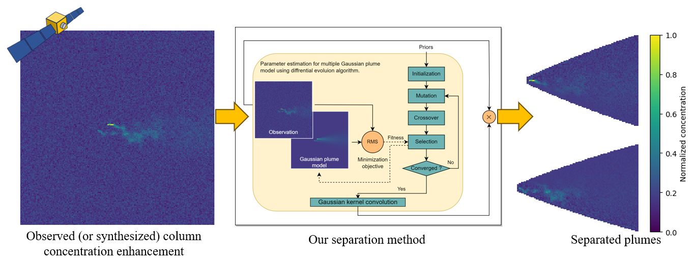
Figure 1 The proposed methodology for separating overlapping plumes. A heuristic-optimization-based method is proposed to estimate the Gaussian plume parameters for each source to separate the overlapping plumes. This method utilizes observed methane column enhancement and auxiliary data with uncertainty as inputs, yielding enhancements of separated plumes. The separated plumes are then quantified with the more precise IME method.

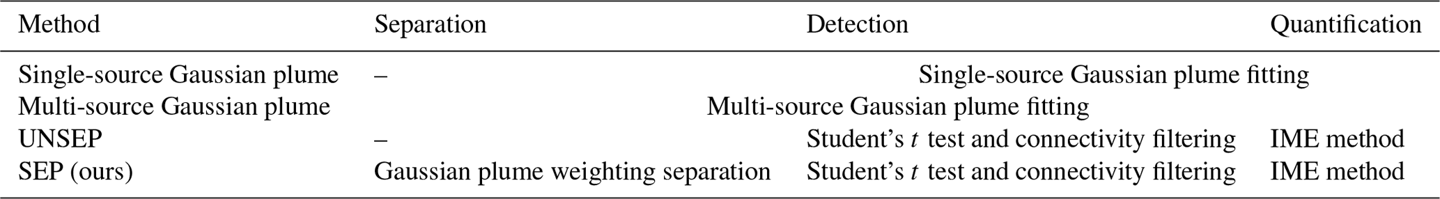
To study the impact of overlapping and the performance of various quantification methods, we simulate plumes using large eddy simulations conducted by the Weather and Research Forecasting Model (WRF-LES; https://www.mmm.ucar.edu/models/wrf, last access: 3 March 2023). Subsequently, we synthesize observations of various sources, meteorological conditions, and observation characteristics based on these simulated plumes. The synthesized observations comprised three scenarios of observation system simulation experiments (OSSEs), including single-source, dual-source, and real scenarios. Within these experiments, we compare the performance of the proposed method in quantification errors against conventional methods (shown in Table 1), including the single-source Gaussian plume method, multi-source Gaussian plume method, and IME method without separation. Furthermore, we validate our method by applying it to a genuine satellite-observed case featuring overlapping plumes.

Table 1 Comparison of methods evaluated in this work.

2 Methods

2.1 Separation and quantification method for overlapping plumes with multiple sources

In this section, a separation and quantification approach is proposed to quantify facility-level methane emissions with overlapping plumes. As shown in Table 1, the proposed method is composed of a Gaussian plume weighting separation process, the plume detection process, and the IME quantification process. Section 2.1.1 describes the formulation of the Gaussian plume models. Section 2.1.2 describes parameter estimation for the Gaussian plume models using a heuristic optimization algorithm. Section 2.1.3 describes the Gaussian plume weighting separation. Section 2.1.4 describes the detection method and the IME quantification method.

Section 2.1.4 describes the combination of the separation method and the IME method for the quantification.

2.1.1 2-D Gaussian plume model

The transport mechanism of methane from point sources in the atmospheric boundary layer (ABL) can be very complicated, as it is affected by multiple factors such as atmospheric turbulence, chemical reactions, and terrain effects. From the perspective of mass conservation, considering wind transport, gradient diffusion, and source–sink terms, the convection–diffusion equation can be obtained to represent this mechanism, which can be written as (Stockie, 2011)

$$\begin{array}{}\text{(1)}& {\displaystyle \frac{\partial C}{\partial t}}+\mathrm{\nabla }\cdot \left(C\mathit{u}\right)=\mathrm{\nabla }\cdot \left(\mathbf{K}\mathrm{\nabla }C\right)+S,\end{array}$$

where C represents the methane column mass concentration at a certain moment; t represents time; u represents the 2-D field of wind velocity vectors; matrix K is diagonal, with its elements representing diffusion coefficients for each wind velocity direction; and S represents the source item.

One way to solve this partial differential equation (PDE) is the numerical method (e.g., Hosseini and Stockie, 2017). However, the computational cost can be enormous. Analytical methods, on the other hand, simplify the problem by making assumptions, allowing for the derivation of analytical solutions to the PDE. For instance, the Gaussian plume expression of a point source can be obtained from the convection–diffusion equation by assuming that the wind speed is constant and uniform, the emission rate is time-invariant, and the turbulence is negligible (Sutton, 1932; Ermak, 1977; Stockie, 2011). The Gaussian plume model is widely applied to describe the pollutants, as well as the GHG dispersion in ABL, particularly in spaceborne GHG monitoring research (Bovensmann et al., 2010; Nassar et al., 2021; Jacob et al., 2022). As a result, we model the column mass concentration (kg m⁻²) at the location (x,y) using a 2-D Gaussian plume model for a ground-level point source, which can be written as (Sutton, 1932; Bovensmann et al., 2010)

$$\begin{array}{}\text{(2)}& {\displaystyle }\begin{array}{rl}{\displaystyle }{C}_{\text{SGP}}& {\displaystyle }(x,y;Q,u)=\\ {\displaystyle }& {\displaystyle \frac{Q}{\sqrt{\mathrm{2}\mathit{\pi }}{\mathit{\sigma }}_y\left(x\right)u}}\exp (-{\displaystyle \frac{\mathrm{1}}{\mathrm{2}}}{\left({\displaystyle \frac{y}{{\mathit{\sigma }}_y\left(x\right)}}\right)}^{\mathrm{2}}),\end{array}\end{array}$$

where the x axis is aligned with the direction of wind speed; Q represents the emission rate (kg s⁻¹); u represents the horizontal wind speed (m s⁻¹) at the plume height; and σ_y represents the diffusion coefficient across-wind, which is a function of downwind distance x and is decided by wind speed, underlying condition, and sunlight (Briggs, 1973). Equation (2) can then be extended to multiple-source scenarios of N sources, and the corresponding concentration is given by

$$\begin{array}{}\text{(3)}& C_{\text{MGP}}(x,y)=\sum _{n=\mathrm{1}}^N{C}_{\text{SGP}}(x_n^{\prime },y_n^{\prime };Q_n,u_n),\end{array}$$

where

$$\begin{array}{}\text{(4)}& \left[\begin{array}{c}{x}_n^{\prime }\\ y_n^{\prime }\end{array}\right]=\left[\begin{array}{cc}\cos {\mathit{\theta }}_n& \sin {\mathit{\theta }}_n\\ -\sin {\mathit{\theta }}_n& \cos {\mathit{\theta }}_n\end{array}\right]\left[\begin{array}{c}x-x_n\\ y-y_n\end{array}\right].\end{array}$$

Here Q_n and u_n denote the emission rate and wind speed of point source n at coordinates (x_n,y_n), respectively, and θ_n represents the wind speed angle of source n in an easting/northing Cartesian coordinate system, where 0 and 90° represent the eastward and northward winds, respectively. We presume uniform wind conditions for the modeled plumes (i.e., u_n=u, ${\mathit{\theta }}_n=\mathit{\theta },\forall n\in \mathrm{1},\mathrm{2},\mathrm{\dots },N$) in this work, given the spatially limited extent of facility-level plumes. This method simplifies subsequent parameter estimation to improve the convergence.

2.1.2 Gaussian plume fitting using the heuristic optimization algorithm

A heuristic optimization algorithm is introduced for parameter estimation of the Gaussian plume model discussed in Sect. 2.1.1. Heuristic optimization algorithms are capable of global searching in optimization and are thus widely used for solving optimization problems. Heuristic optimization algorithms have been widely used in parameter estimation of point source dispersion models (Hutchinson et al., 2017), e.g., Allen et al. (2007), Haupt et al. (2007), and Cervone et al. (2010), showing more robust performance compared to other optimization methods such as Bayesian inference (Platt and DeRiggi, 2012). The differential evolution algorithm (Storn and Price, 1997) is a heuristic optimization algorithm inspired by the evolution theory of biological species.

In this study, the differential evolution algorithm is selected as the estimation algorithm to iteratively minimize the metrics between the modeled concentration image by Eq. (3) and the observed concentration image to estimate the parameters of the dispersion model.

Here, the estimating parameters consist of source locations (x_i,y_i) and emission rates Q_i of source i, the global wind angle θ, and wind velocity u. For the application of the differential evolution algorithm in this paper, the searching spaces for the estimating parameters are set as follows: ±100 m for source locations (x_i,y_i) from their true values; ±50 % for the wind velocity from its true value, which is higher than the average errors of the widely used reanalysis meteorological database analyzed by Varon et al. (2018) and Duren et al. (2019); ±45° for the wind angle θ from its true value; and 0–5000 kg h⁻¹ for emission rates Q_i, covering all methane point sources in Duren et al. (2019).

The minimization objective is also important to apply the optimization algorithm. The most widely used minimization objective is to minimize the root mean square (rms) metrics between modeled and observed concentration images. The rms metric is given as

$$\begin{array}{}\text{(5)}& {\mathcal{L}}_{\text{rms}}=\sqrt{\sum _{i,j}\left(I_{\text{model}}\right(i,j)-I_{\text{obs}}(i,j){)}^{\mathrm{2}}},\end{array}$$

where I_model(i,j) and I_obs(i,j) represent the modeled and observed concentration images, respectively, and i and j represent the pixel indexes in row and column, respectively.

In the application of the differential evolution algorithm, the mutation strategy is set as a best-guided mutation, i.e., DE2 in Storn and Price (1997); the population (NP) is set as $\mathrm{10}\times (N\times \mathrm{3}+\mathrm{2})$, where N represents the number of sources. There are three and two parameters to be estimated for each source and all observations, respectively. The mutation constant (F) is set as 1 and the cross-over constant (CR) is set as 0.9 according to Storn and Price (1997). The relative convergence criterion is set as 10⁻³.

2.1.3 Gaussian plume weighting separation

Figure 1 illustrates the framework to separate an image of overlapping plumes into distinct images, each with a solitary plume. The parameters of the Gaussian plume model are estimated iteratively using the heuristic optimization algorithm described in Sect. 2.1.2, generating a series of images each with its corresponding modeled Gaussian plume. These Gaussian plumes are then utilized as weights to allocate the original observation image pixel by pixel. However, due to the stochastic nature of the transient plume at such small scales, there can be slight misalignments between the modeled Gaussian plume and the transient plume, particularly near the source, which brings obstacles to the following allocation. To address this misalignment issue, we employ Gaussian blur (i.e., convolution with a 2-D Gaussian kernel) to smooth the modeled plumes, thereby increasing robustness against the deviations of the transient plume. Formally, an image with separated plume ${\widehat{I}}_{\text{obs},n}$ of source n from observation I_obs is given by

$$\begin{array}{}\text{(6)}& {\widehat{I}}_{\text{obs},n}=I_{\text{obs}}\cdot {\displaystyle \frac{\langle C_{\text{SGP},n}\rangle }{{\sum }_{p=\mathrm{1}}^N\langle C_{\text{SGP},p}\rangle }},\end{array}$$

where C_SGP,n and C_SGP,p represent the modeled Gaussian plume image of sources n and p, respectively, and 〈⋅〉 represents the Gaussian blur operation.

2.1.4 Plume detection and IME quantification

A transient plume may exhibit significant deviations from the Gaussian plume at small scales, leading to unstable quantification with Gaussian plume fitting. In contrast, the integrated mass enhancement (IME) method demonstrates better accuracy in quantifying small-scale transient plumes (Varon et al., 2018; Jongaramrungruang et al., 2019). Therefore, we employ the IME method for more precise quantification of the separated plumes.

The emission rates estimated by the IME method are given by Varon et al. (2018):

$$\begin{array}{}\text{(7)}& Q={\displaystyle \frac{U_{\text{eff}}\cdot \text{IME}}{L}}={\displaystyle \frac{U_{\text{eff}}\cdot {\sum }_{(x,y)\in \mathbf{I}}\mathrm{\Delta }\mathrm{\Omega }(x,y)A(x,y)}{\sqrt{{\sum }_{(x,y)\in \mathbf{I}}A(x,y)}}},\end{array}$$

where I represents the set of pixels identified as a plume, and ΔΩ(x,y) represents the mass enhancement of pixel (x,y), A(x,y) represents the area of pixel (x,y). The effective wind speed is a logarithmic function with linear variations to 10 m wind speed U₁₀, where the parameters are fitted using the WRF-LES simulations (Varon et al., 2018). Since the IME$/L$ value may vary with the plume pixel detection method, we fit the U_eff for two methods in Table 1, UNSEP and SEP, respectively. We generate a large set of plumes with different emission rates, wind speeds, and mixing heights to fit the U_eff in linear relation to log U₁₀. The result is $U_{\text{eff}}=\mathrm{0.55}\log U_{\mathrm{10}}+\mathrm{0.62}$ m s⁻¹ for UNSEP and $U_{\text{eff}}=\mathrm{0.64}\log U_{\mathrm{10}}+\mathrm{0.94}$ m s⁻¹ for SEP.

The IME method requires the specification of plume pixels I within the observation. Similar to Varon et al. (2018), we utilize a combination of Student's t test and 2-D filters to detect plume pixels in the observation. However, this single-source approach tends to introduce excessive estimation when there is more than one source, thereby hindering comparative analyses between the direct application of IME without separation (denoted as UNSEP) and the proposed separation and quantification approach (denoted as SEP). To mitigate this issue, we propose a straightforward pixel detection process to make the results of UNSEP comparable to SEP. This process, named connectivity filtering, is based on pixel connectivity analysis, a morphological image processing technique. For a source of interest, the pixels in its nearest connected structures are attributed to the source, designated as I, while the remaining detected plume pixels are disregarded.

2.2 Synthesized observation

2.2.1 Methane plume simulation

We perform large eddy simulations using WRF-LES to synthesize observations for the evaluation. The large eddy simulation (LES) is a promising methodology for solving the Navier–Stokes equation and is widely employed to simulate dispersion in the ABL (Stoll et al., 2020). The WRF-LES can perform simulations that show good agreement with observations (Brunner et al., 2023) and is thus widely applied in the field of spaceborne GHG monitoring (Varon et al., 2018; Cusworth et al., 2019; Brunner et al., 2023).

WRF-LES is utilized to simulate 3-D volume concentration of methane (in kg m⁻³) from a point source, where the methane is modeled as a passive tracer (Nottrott et al., 2014). We add a trace gas dispersion function with open boundary conditions by modifying the source code of the WRF 4.4 ideal LES experiment. Similar to Varon et al. (2018), methane plumes are simulated with a mean geostrophic wind of 1, 3, 5, 7, or 9 m s⁻¹; an inversion height of 500, 800, or 1100 m; and a simulation region of 3.5 km×6 km (across and along wind) with horizontal and vertical resolutions of 20 and 10 m, respectively. The initial temperature is set as 293 K in the mixed layer, with a lapse rate of 0.12 K m⁻¹ above the inversion height. The surface sensible heat flux is set as 100 W m⁻². The model is run for 3 h for spin-up and 2 h for registration with 30 s intervals. The trace gas emission rate is set as 1 kg s⁻¹. The simulated concentration is scalable with source emission rates, as simulated by passive trace gas dispersion.

The simulated 3-D volume concentration snapshots are then integrated by weighting each column by a column averaging kernel (Bovensmann et al., 2010; Jongaramrungruang et al., 2019). The column averaging kernel is a vector representing the vertical sensitivity distribution of the instrument and retrieval algorithm, and here it is considered to be vertically uniform. The resulting 2-D column mass enhancements are then subjected to additive Gaussian noise, considering instrumental and retrieval uncertainty. The noise is given as a percentage of methane's mean dry column concentration, which is considered to be 1.8 ppm (i.e., ≈10.3 g m⁻² at 1 atm, dry air). The influence of the methane background is not considered, and the synthesized enhancements are only attributed to plume and noise in this work.

2.2.2 Synthetic observations

To evaluate the possible impact of plume overlapping on quantification and the performance of the proposed separation method, we performed observation system simulation experiments (OSSEs) with simulated mass columns by WRF-LES. OSSEs are widely applied to evaluate spaceborne GHG source detection and quantification abilities by simulating observed spectral radiations or retrieved concentrations (Bovensmann et al., 2010; Kuhlmann et al., 2019; Varon et al., 2018). OSSEs with realistic LESs, accounting for actual surface topography and meteorological conditions (Stoll et al., 2020), are preferable for specific source targets; however, the computational cost can be expensive, considering massive point source targets with highly heterogeneous spatial and emission conditions, e.g., targets in Duren et al. (2019). One feasible approach is to sum multiple simulated column mass images after rotations, shifting, and concentration scalings while assuming the turbulence variations among multiple images are negligible. This approach allows for simulating sources with arbitrary emission rates as well as spatial and meteorological conditions, allowing a much lower computational cost and thus reducing linear time complexity (O(N)) to nearly constant (O(1)) for simulating N sources when N is large enough.

To synthesize an image of concentration enhancement observation with multiple sources, we first establish an easting/northing Cartesian system where the x axis points east and the y axis points north. The field of view (FoV) is square with sides of length 6 km and parallel to the axes, centered at (0,0) of the Cartesian system. Then, the 2-D column mass snapshots are randomly selected with the given wind speed and mixing depth. These snapshots are then scaled according to the emission rate of each source. Then, to rotate and shift the snapshots for an observation, we traverse all the pixels in the observation and accumulate their mapping pixels in each snapshot. For a given pixel of the observation at (x,y), the mapping pixel indexing in the nth snapshot is given by

$$\begin{array}{}\text{(8)}& {\displaystyle }\begin{array}{rl}{\displaystyle }\left[\begin{array}{c}{i}_n^{\prime }\\ j_n^{\prime }\end{array}\right]=& {\displaystyle }\left[\begin{array}{cc}\cos \mathit{\theta }& \sin \mathit{\theta }\\ -\sin \mathit{\theta }& \cos \mathit{\theta }\end{array}\right]\left[\begin{array}{c}x-x_n\\ y-y_n\end{array}\right]\cdot \left[\begin{array}{c}\frac{\mathrm{1}}{\mathrm{\Delta }x}\\ \frac{\mathrm{1}}{\mathrm{\Delta }y}\end{array}\right]\\ {\displaystyle }& {\displaystyle }+\left[\begin{array}{c}{I}_{\text{source}}\\ J_{\text{source}}\end{array}\right],\end{array}\end{array}$$

where θ represents the wind angle to the x axis, (x_n,y_n) represents the location of source n, Δx and Δy represent the horizontal resolutions in WRF-LES, and (I_source,J_source) represents the location of the source pixel in WRF-LES. The indices $(i_n^{\prime },j_n^{\prime })$ are then rounded, thus completing the nearest-neighbor interpolation. Here, considering the small size of the plume and the domain, we adopt a unified wind velocity across the domain.

2.2.3 Observation scenarios

We test our separation method under three different scenarios, namely Exp1–3, each consisting of trials with various experiment settings. Examples of each scenario are shown in Fig. 2. Exp1, the single-source scenario, comprises a full factorial experiment of environmental factors, source factors, and observation factors to evaluate the performance of quantifying methods. Exp2, the dual-source scenario, comprises a full factorial experiment with several overlapping-related factors to analyze the impact of plume overlapping, as well as to evaluate the performance of separation and quantification methods. Exp3, the random source scenario, comprises a Monte Carlo test to further evaluate the separation and quantification methods.

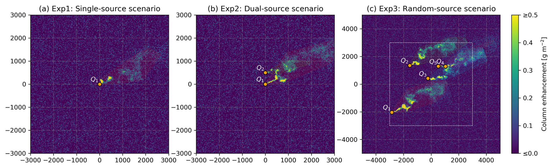
Figure 2 Examples for each experiment scenario of synthesized observations. The plots represent the synthesized methane column enhancements. Each semi-transparent polygon patch covers a plume, where the concentration is larger than the uncertainty. The dashed box in (c) encloses the area where random sources are generated. The emission rates vary between 200 and 2000 kg h⁻¹. In these examples, the ground pixel size is fixed at 25 m, while the retrieval uncertainty is set at 1 %.

In Exp1, a single source is placed in the center of the simulation domain and a full factorial experiment is conducted to test the performance of the quantifying method under all combinations of multiple-factor levels. These factors include environmental factors (mixing depth at 500, 800, and 1100 m; wind speed at 1, 3, 5, 7, and 9 m s⁻¹; wind direction at 0 and 45°), source factors (emission rates ranging from 100 to 2000 kg h⁻¹), and observation factors (ground pixel size ranging from 25 to 200 m; retrieval uncertainty at 1 %, 3 %, and 5 %). It is noteworthy that for observation factors, ground pixel size is determined by typical point source monitoring satellites, while retrieval uncertainty is established by satellites with ultrafine spectral resolution, such as GHGSat (Varon et al., 2018). The wind direction is defined in the Cartesian coordinate system, and the retrieval uncertainty is considered a 0-biased additive noise with the standard deviation as a percentage of methane's mean dry column mass. Each combination is repeated 10 times. The quantification performance of the Gaussian plume fitting, unseparated IME (UNSEP), and separated IME (SEP) methods is evaluated. The results are elaborated in Sect. 3.1. Examples of the plume image under various conditions are shown in the Supplement.

In Exp2, a secondary source is introduced as an interference source to produce overlapping in order to evaluate the impact on quantification and separation. Exp2 is also a full factorial experiment, where we fix the mixing depth at 800 m, the emission rates at 200 kg h⁻¹, the ground pixel size at 25 m, and the retrieval uncertainty at 1 %. The rest of the factors include wind speed at 1, 3, 5, 7, and 9 m s⁻¹; wind direction ranging from −90 to 90°; distance ranging from 100 to 900 m; and the emission rate ratio between the secondary and original source ($Q_{\mathrm{2}}/Q_{\mathrm{1}}$) ranging from 0 to 5. Each combination of trials is repeated 10 times. The quantification performance of the single-source Gaussian plume fitting, multi-source Gaussian plume fitting, unseparated IME, and separated IME methods is evaluated. The results are elaborated in Sect. 3.2. Comparable results with different ground pixel size and noise settings are shown in the Supplement.

In Exp3, a Monte Carlo experiment is conducted to further assess the performance of the unseparated IME and separated IME methods. For each trial, one source is randomly sampled from the AVRIS-NG observed methane source list (Duren et al., 2019), and its geolocation and emission rate are thus specified. Likewise, additional neighboring sources within the 6 km×6 km domain are then included in the simulation. For simplicity, sources with emission rates lower than 25 kg h⁻¹ (accounting for about 5 % of the summation) are excluded from the list as they are considered too small to be accurately measured by spaceborne measurements, and their interference as background is also neglected. Additionally, we assume all the sources on the list exhibit persistence. This assumption is supported by the average confidence for persistence on the original list being 0.83. Additionally, it compensates for the manual removal of overlapping sources during the quality control phase conducted by the list maker. The winds to load the plumes are then obtained from the 10 m wind of the fifth generation of atmospheric reanalysis of the European Centre for Medium-Range Weather Forecasts (ECMWF ERA5; Hersbach et al., 2020). We then match geostrophic wind using the 10 m wind (shown in the Supplement). A random plume with the matched geostrophic wind is then added to the domain. The sampling time range for loading wind velocity covers local noon in 2022. The wind velocity is considered uniform across the domain and is interpolated to the observation center using five-point inverse distance weighting such as in Xu et al. (2022). To ensure that all generated sources inside the domain are quantifiable, each side of the simulation frame is extended outward 2 km for a 10 km×10 km domain. The plumes originating from outside the domain are considered well mixed and their interferences with the synthesized enhancements are not considered. This random experiment is repeated 2000 times. The quantification performances of the unseparated IME and separated IME methods are then evaluated and elaborated in Sect. 3.3.

2.3 EMIT observation

We also test our separation method on methane plumes retrieved by the Earth Surface Mineral Dust Source Investigation (EMIT) instrument installed on the International Space Station (ISS). EMIT is a hyperspectral instrument capable of imaging spectroscopy in the visible to short wavelength infrared, with a nadir ground sampling distance of 30–80 m (Green et al., 2020). The methane column enhancement data (EMITL2BCH4ENHv001) are expressed in units of parts per million meters (ppm m) and are retrieved using an adaptive matched filter technique (Green et al., 2023b). Green et al. (2023a) also provide the corresponding identified plume complexes (EMITL2BCH4PLM v001), where the plumes sometimes overlap and thus form these clusters.

For the quantification, we first converted the concentration map from ppm m to kg m⁻² (Sánchez-García et al., 2022). Then, we applied the separation method to extract plumes from each source, and the extracted plumes were then quantified by the IME method, as described in Sect. 2.1. The wind velocity for separation and quantification is interpolated from ERA5 as described in Sect. 2.2.3. The source locations are identified through visual inspection and cross-verified with local ground facilities using a high-resolution satellite map from Google Earth. Monte Carlo propagation is introduced to evaluate the uncertainty of the quantification, and the systematic uncertainty of the IME method is not considered (Sánchez-García et al., 2022). For the Monte Carlo propagation, the input uncertainties include observation uncertainty from the corresponding EMITL2BCH4PLM data and wind speed uncertainty estimated as the standard deviation of the five points nearest ERA5.

2.4 Evaluation indicators

2.4.1 Overlapping indicator

To assess the degree of plume overlapping, a mass overlapping index is proposed, defined as the ratio of the mass integration of the interference sources to that of the primary source. The mass overlapping index for source i of N sources is given by

$$\begin{array}{}\text{(9)}& {\displaystyle }\begin{array}{rl}{\displaystyle }& {\displaystyle }{\text{OI}}_{{\text{mass}}_i}=\\ {\displaystyle }& {\displaystyle \frac{{\sum }_{(x,y)\in \mathbf{I}}\left[\right({\sum }_{n=\mathrm{1}}^N\mathrm{\Delta }{\mathrm{\Omega }}_n(x,y)-\mathrm{\Delta }{\mathrm{\Omega }}_i(x,y))\cdot A(x,y\left)\right]}{{\sum }_{(x,y)\in \mathbf{I}}\mathrm{\Delta }{\mathrm{\Omega }}_i(x,y)A(x,y)}},\end{array}\end{array}$$

where I denotes the plume pixel of source i. Higher ${\text{OI}}_{{\text{mass}}_i}$ means that the plume of source i is subject to more severe interference.

2.4.2 Emission rates estimation indicators

The quantification of a methane source is considered equivalent to solving a parameter estimation problem. We introduce R², the coefficient of determination, to indicate the overall prediction accuracy. Furthermore, as R² has a relatively poor ability to explain samples with small true values, absolute percentage error (APE) is introduced to indicate the estimation error of a single sample, and mean absolute percentage error (MAPE) is introduced to indicate the overall estimation error. The definitions of R², APE, and MAPE are given by

$$\begin{array}{}\text{(10)}& {\displaystyle }{R}^{\mathrm{2}}=\mathrm{1}-{\displaystyle \frac{{\sum }_{n=\mathrm{1}}^N({\widehat{Q}}_n-Q_n{)}^{\mathrm{2}}}{{\sum }_{n=\mathrm{1}}^N(\stackrel{\mathrm{‾}}{Q}-Q_n{)}^{\mathrm{2}}}},\text{(11)}& {\displaystyle }{\text{APE}}_n=\left|{\displaystyle \frac{{\widehat{Q}}_n-Q_n}{Q_n}}\right|,\text{(12)}& {\displaystyle }\text{MAPE}={\displaystyle \frac{\mathrm{1}}{N}}\sum _{n=\mathrm{1}}^N\left|{\displaystyle \frac{{\widehat{Q}}_n-Q_n}{Q_n}}\right|,\end{array}$$

respectively, where Q_n and ${\widehat{Q}}_n$ represent the true emission rate and predicted emission rate, respectively, of source n; $\stackrel{\mathrm{‾}}{Q}$ is the average of true emission rates; and N represents the number of sources in the experiments.

3 Results

3.1 Quantification results for a single source

In Exp1, we evaluate the baseline performance of various quantification methods, including the emission rates derived directly from the Gaussian plume fitting, unseparated and direct IME quantification (denoted as UNSEP), and quantification after applying the separation method (denoted as SEP) using a full factorial experiment. The overall quantification errors (MAPE) for the three quantification methods are 0.89, 0.30, and 0.40, respectively. The distributions of quantification errors, in terms of absolute percentage error (APE), with respect to different simulation factors in Exp1 are shown in Fig. 3.

Figure 3 Distribution of quantification APE under various experimental parameters in Exp1. The orange dashes denote the medians of APE, the boxes denote the range between the lower and upper quartiles (Q1 and Q3), and ⊥ and ⊤ extend from the box by 1.5 times the interquartile range (IQR). The quantification errors in APE of Gaussian plume fitting, unseparated IME (UNSEP), and separated IME (SEP) methods are represented in the legend.

As shown in Fig. 3a, the APE of all three methods exhibits nearly linear increasing trends with respect to pixel size, with Pearson's correlation coefficients (R) of 0.24, 0.18, and 0.21, and all p values are less than 0.01. Similar trends are also shown in Fig. 3b, where the APE of three methods increases slightly with respect to uncertainty ($R=\mathrm{0.16},\mathrm{0.13},\mathrm{0.14}$; p<0.01). As shown in Fig. 3c and d, the variance of APE with respect to mixed depth and wind direction is minor. As shown in Fig. 3e, the APE of the Gaussian plume and UNSEP increases with respect to the wind speed. However, the APE of the SEP reaches the maximum at the wind speed of 3 m s⁻¹. With increasing wind speed, SEP exhibits lower quantification error than UNSEP of 9 m s⁻¹. As shown in Fig. 3f, the quantification error of all three methods decreases with the emission rates and shows a sublinear trend.

3.2 Quantification results for dual sources

In Exp2, we introduce an interference source to create overlapping for the full factorial experiment. After introducing an interference source, the MAPE of single-source Gaussian plume fitting increases from 0.45 to 1.23, while the increases in the multi-source Gaussian plume model are negligible, which remain 0.45. Similarly, the UNSEP increases from 0.15 to 0.83, while the SEP only increases from 0.30 to 0.38.

As demonstrated in Fig. 4, the SEP shows the best quantification performance in most cases, followed by multi-source Gaussian plume fitting, UNSEP, and single-source Gaussian plume fitting in terms of MAPE. With decreasing wind speed, the errors of quantification results by multi-source Gaussian plume fitting become comparable to that of SEP. When the wind speed is 1 m s⁻¹, the quantification results of multi-source Gaussian plume fitting are slightly better than SEP. As distance increases or interference strength ($Q_{\mathrm{2}}/Q_{\mathrm{1}}$) decreases, plumes are less likely to overlap, leading to UNSEP outperforming SEP. At 900 m distance or interference strength decreasing to 0.5, UNSEP achieves the best quantification performance.

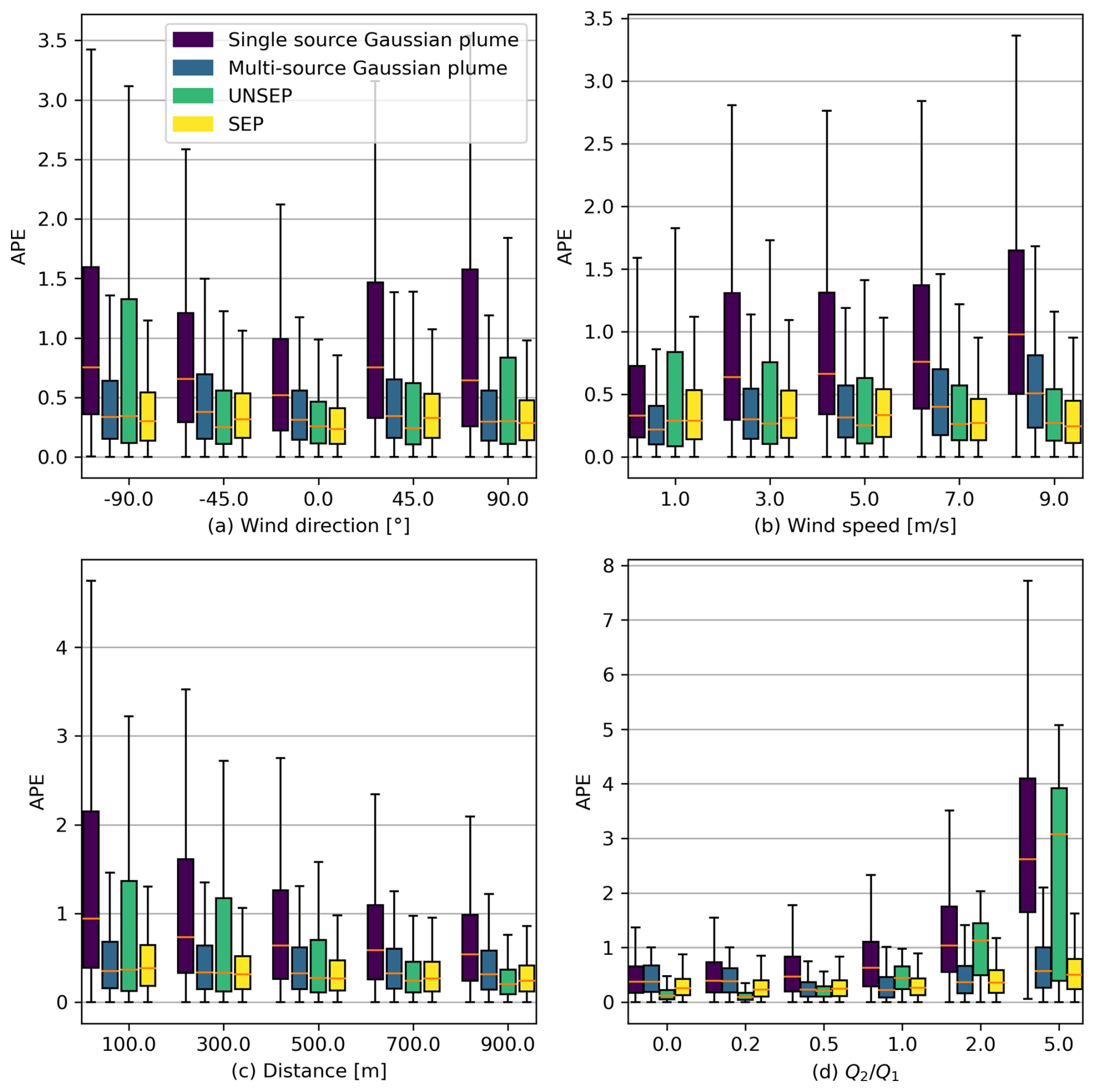
Figure 4 Distribution of quantification APE with respect to various experimental factors in Exp2.

The multiple-source Gaussian plume and SEP exhibit better quantification performance on overlapping plumes as interference strength intensifies. Also, both multi-source Gaussian plume fitting and SEP show minor variations in factors including wind direction, wind speed, distance between two sources, and interference strength. In contrast, single-source Gaussian plume fitting and UNSEP are more susceptible to these factors, with their performances deteriorating as wind direction increasingly aligns with the line connecting the sources, wind speed decreases (for UNSEP), wind speed increases (for single-source Gaussian plume fitting), distance decreases, and interference intensifies. Similar trends are observed with varying observation pixel sizes and retrieval noise, as demonstrated in our further experiments (shown in the Supplement).

3.3 Quantification results for random sources

In Exp3, we focus on comparing the UNSEP and SEP in a more realistic Monte Carlo simulation. Factors including source locations, emission rates, and wind velocities are randomly selected from real distributions. The sampled factors demonstrate good agreement in terms of source emission rates (Fig. 5a) and wind speed (Fig. 5b) with the real distributions of the entire source list. The sampled emission rates follow a lognormal distribution, with a mean of 172.2 kg h⁻¹ and standard deviation of 340.8 kg h⁻¹. As shown in Fig. 5c, 53.7 % of the frames cover one source, 24.6 % of the frames cover two sources, and 21.7 % of the frames cover more than two sources. On average, there are 2.33 sources per frame (6 km×6 km).

Figure 5 Statistical description of the factors in the Monte Carlo experiment (Exp3). The red bins denote the distribution of all sources from the AVIRIS-NG methane source inventory and the corresponding local noon wind speed distribution in the entire year of 2022. The blue bins denote the distribution of the selected sources in Exp3.

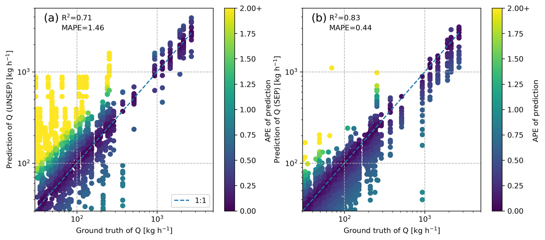
Figure 6 Comparison between quantification results of (a) unseparated quantification and (b) separated quantification in Exp3.

Figure 6 shows the quantification results of unseparated and separated IME quantifications. The results of SEP demonstrate improvements in R² from 0.71 to 0.83 compared to UNSEP and a decrease in the quantification error (MAPE) from 1.46 to 0.44. We also find that SEP is notably more accurate in estimating low-emission sources compared to UNSEP.

To further investigate the distribution of overlapping and the performance of UNSEP and SEP in handling overlapping, we demonstrate quantification error over the source overlapping index (shown in Fig. 7). The overlapping index OI_mass ranges from 0 to 6.09. Only 36.0 % of sources are completely isolated from other sources, and their overlapping index OI_mass is 0; half of the sources have OI_mass>0.02, and 4.3 % of sources are subjected to overlapping with OI_mass≥1. We observe a nearly linear relation relationship between APE of UNSEP and OI_mass (Pearson's R=0.45, p<0.01), and the regression result can be expressed as ${\text{APE}}_{\text{UNSEP}}=\mathrm{2.76}\cdot {\text{OI}}_{\text{mass}}+\mathrm{1.34}$. We define severe overlapping as occurring when the APE exceeds twice the intercept. Then, this results in an OI_mass threshold of 0.41, indicating that 28.9 % of the sources experience severe overlapping. In comparison, the corresponding OI_mass threshold of SEP is 3.00 (${\text{APE}}_{\text{SEP}}=\mathrm{0.15}\cdot {\text{OI}}_{\text{mass}}+\mathrm{0.45}$; Pearson's R=0.13, p<0.01), which only accounts for 0.5 % of all sources. This indicates that the effect of overlapping is largely suppressed by SEP and thus results in robust quantification.

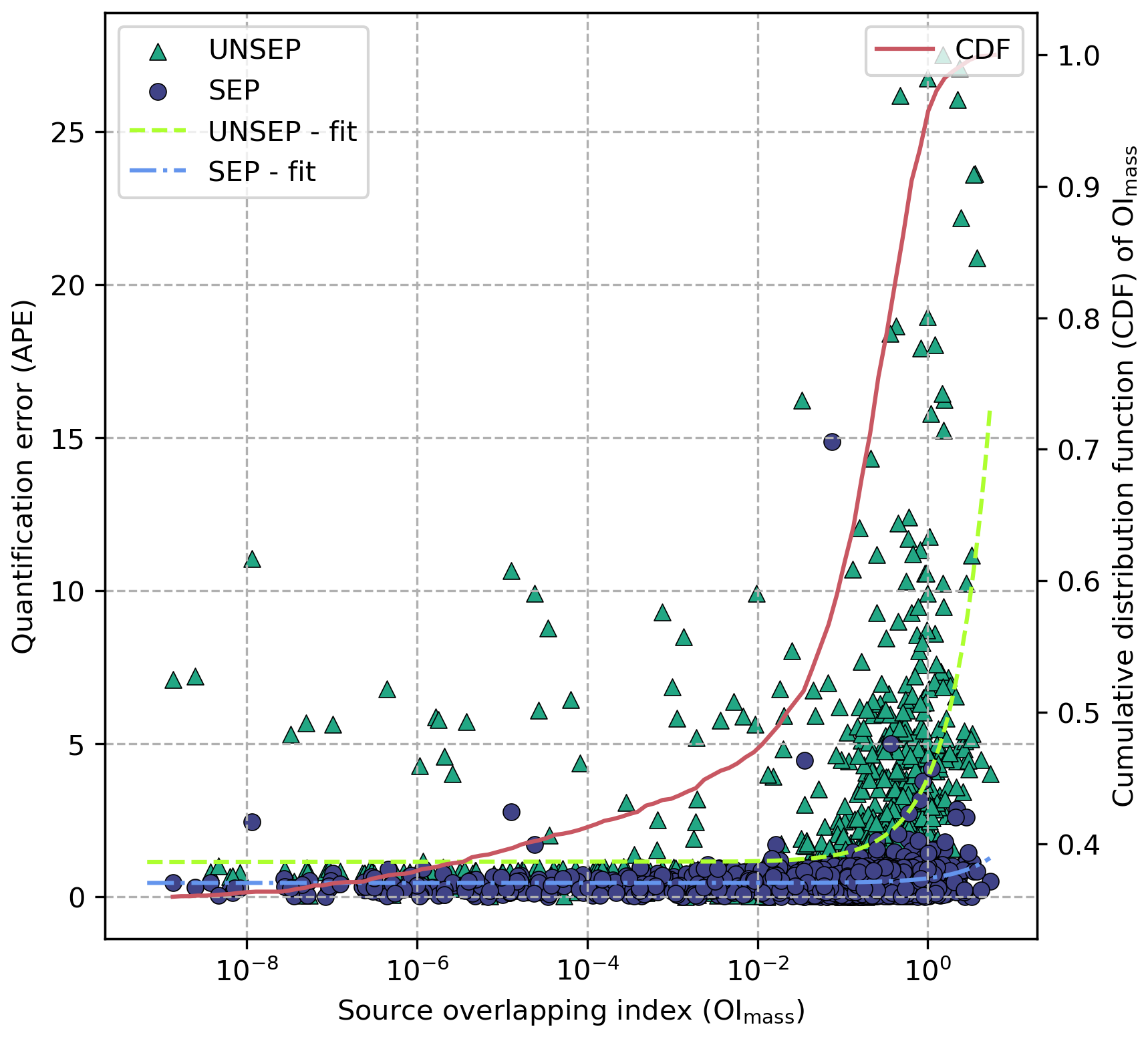
Figure 7 Comparison between quantification results and the source overlapping index (OI_mass). The dashed line represents the linear fitted quantification error of UNSEP with respect to OI_mass. The solid red line represents the cumulative distribution function of OI_mass.

3.4 Quantification on EMIT observation

In this section, we evaluate our separation and quantification method using real satellite observations of EMIT. We focus on a specified cluster of plumes observed by EMIT on 15 August 2022 at 04:28 UTC in Turkmenistan, near the Goturdepe oil and gas production field. The sources in this location are spatially aggregated and create significant plume overlapping (see Fig. 8). Through manual inspection and high-resolution satellite imagery verification, we identify six sources within the cluster. The emission rates of each source are quantified using our separated quantification method. Additionally, we quantify the entire cluster as a whole using the conventional IME method (UNSEP without connectivity filtering in Sect. 2.1.4).

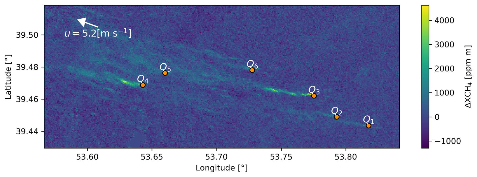
Figure 8 Overlapping plumes observed by EMIT on 15 August 2022 at 04:28 UTC. This image is from the dataset EMITL2BCH4ENH v001, which is publicly available at https://lpdaac.usgs.gov/products/emitl2bch4enhv001/ (last access: 3 July 2024).

The quantification results are shown in Table 2. The estimated emission rates for each source range from 1.64 to 5.20 t h⁻¹. We compare our estimated emission rates with previous research. We find that source Q₃ has also been quantified by Irakulis-Loitxate et al. (2022) and Sánchez-García et al. (2022), and their estimations for Q₃ are 1.4 ± 0.4 and 5.0 ± 2.2 t h⁻¹, respectively. There is a gap of more than 2 years between these two estimations, and their estimations demonstrate significant differences. Our estimation for Q₃ on 15 August 2022 is 3.34 ± 0.90 t h⁻¹, which is comparable to the previous estimations. The summation of separated quantification results for the six sources is 16.77 ± 4.65 t h⁻¹. In comparison, the quantification result of the whole cluster is 21.06 ± 5.51 t h⁻¹, which is higher than the summation, but their differences are consistent within margins of error. This is reasonable as pixels in separated quantification may not be attributed to any source and thus excluded in the final quantification, leading to underestimations.

Table 2 Quantification results from EMIT observations. Six sources are manually identified and quantified. The quantification result summation for the separated IME method over each source separately (summation) is compared to the results for the unseparated IME method over the whole methane plume cluster (whole).

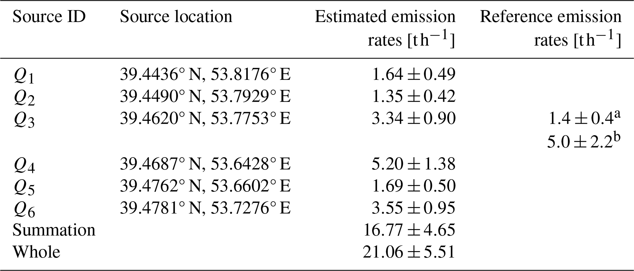
^a Observed by PRISMA on 27 March 2020 (Irakulis-Loitxate et al., 2022). ^b Observed by WorldView-3 on 10 April 2022 (Sánchez-García et al., 2022).

4 Discussion and conclusions

In this study, we compared the baseline quantification performance of the Gaussian plume model with two IME-based methods (UNSEP and SEP) for spaceborne methane point source monitoring in Exp1 (see Sect. 3.1). Our findings indicate that the IME methods outperform the Gaussian plume model on small scales with ground pixel sizes up to 200 m. Additionally, we observed weak positive linear relationships of the quantification error of all three methods with respect to both ground pixel size and retrieval uncertainty.

Then we investigated the impact of plume overlapping on the quantification. We found that plume overlapping increases quantification errors in Exp2. Specifically, the MAPE for the UNSEP method increased from 0.15 to 0.83, and for single-source Gaussian plume fitting, it increased from 0.45 to 1.23 when compared to cases with no interference (see Sect. 3.2). Factors such as closer source intervals and disproportion emission rates will enlarge these defects. Overlapping plumes can produce connective pixels that cover multiple sources, which are ambiguous to attribute. Simply eliminating these pixels will result in increasing missed detections and quantification errors. In addition, the relatively sparse spatial resolution of spaceborne methane monitoring techniques compared to airborne techniques can increase the proportion of these ambiguous pixels. The findings from the Monte Carlo experiment in Exp3 indicate that plume overlapping can affect up to 18 % of the sources, resulting in a doubling of errors for unseparated IME quantification (see Sect. 3.3). As a result, it is essential to find and attribute pixels in overlapping plumes correctly for spaceborne quantification.

To tackle this issue, we introduced a heuristic optimization algorithm to perform parameter estimations for the 2-D multi-source Gaussian plume model. Based on the outputs of this model with the estimated parameters, we assigned the mass to sources according to the modeled concentrations by each pixel. In this way, we separated an overlapping plume image into several single-plume images. This “soft segmentation” shows better performance in plume pixel detection for overlapping plumes than “hard segmentation” methods, e.g., the plume detection method by Varon et al. (2018), which assigns all the mass in a pixel to a single source while the mass may originate from multiple sources. Results in the Monte Carlo experiment (Exp3) show that the application of separation is effective in quantification, where MAPE decreases from 1.46 to 0.45, and R² increases from 0.71 to 0.84, compared to quantification without separation (see Sect. 3.3).

Additionally, our separation model can perform independent estimation for attributes such as wind speed and direction, as well as source locations, which makes the separation robust to the uncertainty in auxiliary data. Although the emission rates as parameters of the 2-D multi-source Gaussian plume model are estimated, they are only used for separation instead of quantification. As our experiment results in Exp1 and Exp2 show, Gaussian plume fitting exhibits higher systematical uncertainty than the IME method in quantifying fine-scale methane plumes. It needs to be noted that, in our experiment, the quantification error of the Gaussian plume increases with pixel size and is constantly higher than the IME methods as shown in Exp1. This is slightly different from Varon et al. (2018) and Jongaramrungruang et al. (2019), who demonstrate that the plume shows a better approximation of Gaussian form with increasing pixel size above 300 m. One explanation for the inability to pinpoint the turning point of performance enhancement in Gaussian plume fitting is the limited size of our simulation domain. As we increase the pixel size, the number of pixel samples decreases, which counteracts the advantages of averaging eddies using larger pixels, thereby impeding the performance improvement of the Gaussian plume fitting. A comprehensive exploration of the trade-offs between Gaussian plume and IME methods may require large-scale, high-resolution LESs and is beyond the scope of this paper.

In the experiment with real satellite observations (see Sect. 3.4), firstly, we notice that identifying source locations correctly is crucial for separation and quantification. Although we verified the source with satellite imagery, it still appears less precise. Utilizing detailed facility-level inventories, such as VISTA-CA, could greatly help source detection, separation, and quantification. Additionally, for previously unknown emission sources, integrating multimodal information, including pipeline maps, and using simultaneous facility flare observations can also be introduced for accurate identification (Irakulis-Loitxate et al., 2022). Secondly, we also notice that there are unignorable differences in source quantification results across research, as shown in Sect. 3.4. The temporal variability in source emissions and the associated uncertainty in quantification are coupled, posing challenges to cross-verification among observations. This suggests the need for further verification with ground-truth data. Thirdly, we find that in some cases the plumes exhibit a large deviation from the WRF-LES simulation, especially in complex terrains, such as valleys. In this case, using uniform wind assumptions may also lead to the overestimation of the performance of the IME quantification method as well as the separation method.

In this study, we proposed a separation and quantification approach, which combines the Gaussian plume and IME method, to quantify overlapping plumes from multiple facility-level point sources in spaceborne methane observations. As implied by the VISTA-CA inventory and AVIRIS-NG observed methane source list, the methane point sources can be spatially aggregated in some places, meaning that the plume overlapping may be non-negligible. This deficiency will constrain the quantification scope of spaceborne GHG monitoring techniques. As a result, our separation method can be important to spaceborne methane monitoring for constructing or verifying facility-level emission inventories (e.g., Duren et al., 2019), as well as environmental administration departments. For future research, a dispersion model, which is more representative of real transient plumes, can be introduced to improve the separation performance. The interferences of background methane are not considered in this work, and future work may consider using realistic backgrounds to account for irregular noise, such as Jongaramrungruang et al. (2022) and Gorroño et al. (2023). A series of tests on more realistic simulations, as well as real observations, should also be performed for further validation.