High-resolution maps of Arctic surface skin temperature and type retrieved from airborne thermal infrared imagery collected during the HALO–(𝒜 𝒞)³ campaign

Two retrieval methods for the determination of Arctic surface skin temperature and surface type based on radiance measurements from the thermal infrared (TIR) imager VELOX (Video airbornE Longwave Observations within siX channels) were developed. VELOX captured TIR radiances in terms of brightness temperatures for wavelengths from 7.7 to 12 µm in six spectral channels. The imager was deployed on the High Altitude and LOng Range research aircraft (HALO) during the HALO–(𝒜𝒞)³ aircraft field campaign conducted in the framework of the Arctic Amplification: Climate Relevant Atmospheric and SurfaCe Processes and Feedback Mechanisms (𝒜𝒞)³ research programme. The measurements were taken over the Fram Strait and the central Arctic in March and April 2022. Radiative transfer simulations assuming cloud-free atmospheric conditions were performed showing that the influence of water vapour on the measured brightness temperature can be neglected. Therefore it was possible to apply a single-channel retrieval technique to obtain the surface skin temperature from the VELOX data. The retrieval results were compared with data from the MODerate-resolution Imaging Spectroradiometer (MODIS) showing an agreement within 2.0 K. Secondly, a pixel-by-pixel surface classification retrieval was developed using a random forest algorithm. It classifies surfaces into types of open water, sea-ice–water mixture, thin sea ice, and snow-covered sea ice. The resulting sea-ice concentrations were compared with satellite data, yielding a mean absolute difference (MAD) of 5 %. In addition, the classified pixels were aggregated into segments of the same surface type, providing different segment size distributions for all surface types. When grouped by the distance to the sea-ice edge, the segment size distribution showed a shift to fewer but larger floes in the direction of the pack ice.

1 Introduction

Arctic amplification comprises Arctic-specific processes and feedback mechanisms that cause a number of obvious changes of the Arctic climate system, such as accelerated warming of the Arctic region as compared to the rest of the globe (Wendisch et al., 2023a). Another signature of Arctic amplification involves the transition to fewer, thinner, and more dynamic sea ice within the last decades (Kwok, 2018; Meier and Stroeve, 2022; Budikova, 2009; Notz and Community, 2020). Therefore, observations of the current state and the changes of the Arctic sea ice are critical. Furthermore, the Arctic sea ice serves as a thermal insulator, regulating heat and moisture exchange between the ocean and atmosphere (Maykut and Untersteiner, 1971; Qu et al., 2019). To quantify these exchange processes, measurements of sea-ice surface skin temperature (IST) and open-ocean sea surface temperature (SST) are crucial. In situ measurements from buoys or ship-borne instruments are sparse in the Arctic due to harsh conditions and logistical challenges in this area (Smith et al., 2019). As a consequence, remote sensing techniques are used to determine IST and SST (Hall et al., 2004; Li et al., 2022; Nielsen-Englyst et al., 2023). To retrieve these properties, established approaches use information supplied by observations in the wavelength range of the atmospheric window (7–14 µm), where atmospheric absorption can mostly be neglected (McMillin and Crosby, 1984; Liu et al., 2006). Specifically, wavelength bands centred around 11 and 12 µm are commonly used to retrieve the temperature of prevailing surface features (Hall et al., 2004). However, in the Arctic, these surface features partly represent small-scale phenomena, such as leads, which are narrow openings in sea ice with spatial extents ranging from metres to kilometres. Leads may account for a significant amount of net heat energy fluxes in the Arctic (Qu et al., 2019; Gryschka et al., 2023). Additionally, melt ponds, which form on sea ice due to melting processes, reduce the surface albedo by up to 45 % (Tao et al., 2024), thereby affecting the solar atmospheric radiative energy budget significantly close to the ground (Anhaus et al., 2021; Niehaus et al., 2023). Common satellite retrievals often lack the horizontal resolution needed to discriminate the majority of narrow leads and small melt ponds. For example, the horizontal resolution of the MODerate resolution Imaging Spectroradiometer (Willmes and Heinemann, 2015, MODIS) restricts its observations to features larger than 500 m (Hall et al., 2004). The heterogeneous spatial distribution of typical Arctic surface types, e.g. open water, thin sea ice, snow-covered sea ice, melt ponds, and transitional types plays an important role in the determination of the Arctic Radiative Energy Budget (REB) (Di Biagio et al., 2021; Anhaus et al., 2021; Wendisch et al., 2023b).

To quantify spatial heterogeneity, surface classification algorithms have been developed, using empirically determined thresholds (Massom and Comiso, 1994; Jäkel et al., 2019b; Thielke et al., 2023), including supervised (Wright and Polashenski, 2018) and unsupervised statistical learning approaches (Paul and Huntemann, 2021). Massom and Comiso (1994) used measurements at wavelengths in the thermal infrared (TIR) from the Advanced Very High Resolution Radiometer (Cracknell, 1997, AVHRR) to classify the surface into open water, new ice, young ice, and thick ice with a snow cover with a resolution of 1.1 km at nadir. The scene classification by Paul and Huntemann (2021) used MODIS TIR data with wavelengths similar to Massom and Comiso (1994), but the classification into open water, thin sea ice, thick sea ice, and clouds was performed by a deep neural network instead of thresholds based on a histogram. As both approaches used TIR data, they can also be applied at polar night. In contrast, Jäkel et al. (2019b), Thielke et al. (2023), and Wright and Polashenski (2018) relied on high-spatial-resolution airborne data rather than satellite imagery. While Thielke et al. (2023) used a thermal imager mounted to a helicopter during polar night, both Wright and Polashenski (2018) and Jäkel et al. (2019b) derived surface type classifications with airborne based measurements at visible wavelengths to distinguish open water, melt ponds, and sea ice. Thielke et al. (2023) retrieved IST to distinguish sea ice and open water with a resolution of 1 m and Wright and Polashenski (2018) used imagery on the decimetre scale. In summary, results of satellite retrievals offer wide scene and consistent time coverage but provide data with limited horizontal resolution, while airborne data offer images of high horizontal resolution but with limited spatial and temporal coverage.

Therefore, we have developed a skin temperature retrieval algorithm applied to the TIR imager VELOX (Video airbornE Longwave Observations within siX channels; Schäfer et al., 2022) and combined with a surface type classification using supervised machine learning techniques. A random forest algorithm (Breiman, 2001; Belgiu and Drăguţ, 2016; Wright and Polashenski, 2018) was used to classify the observed surface types pixel-by-pixel into four categories: open water (OW), ice–water mix (IWM), thin ice (TI), and snow-covered ice (SC). To sharpen the interpretation of spatial properties of the surface types, a segmentation was applied unifying neighbouring pixels of the same surface type into segments. The article is structured as follows: the measurements from the HALO–(𝒜𝒞)³ campaign and satellite data used in this study are introduced in Sect. 2. The single-channel surface skin temperature retrieval method and the random forest algorithm used to classify surface types are described in Sect. 3. The data are used to investigate the spatial characteristics of the classified surface types in Sect. 4.

2 Measurements and instrumentation

2.1 Airborne campaign

The HALO–(𝒜𝒞)³ aircraft campaign was conducted from 7 March to 12 April 2022 to investigate the evolution of air mass transformation processes during warm-air intrusions and cold-air outbreaks in the Arctic (Wendisch et al., 2024). In total, 59 flights with multiple research aircraft were realized, among them 17 flights with research aircraft HALO, which was based in Kiruna, Sweden. In Fig. 1, the locations of measurement are depicted, together with the campaign-averaged sea-ice concentration (SIC). In addition to all HALO tracks that were flown during the campaign (limited to the map extent; for a full overview see Wendisch et al., 2024).

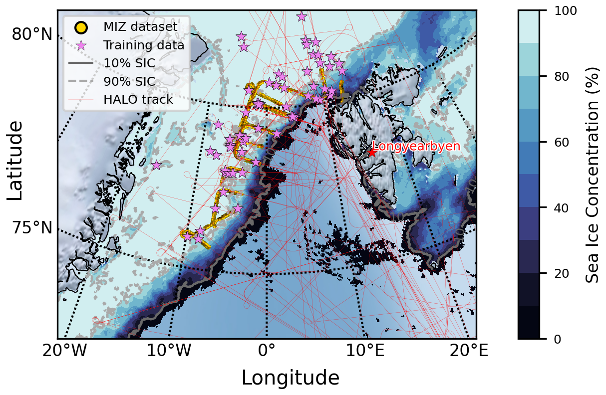
Figure 1 Overview of the data applied in this study, with the location of the data points in orange and all flown HALO tracks in light red. The average SIC during the campaign is shown in blue contours, with a grey solid and dashed line indicating the 10 % and 90 % SIC contour, respectively. The data were provided by Spreen et al. (2008). Pink stars indicate the location of the training data used for the supervised classification.

Due to HALO's range of up to 9000 km, the measurements capture Arctic surface and atmospheric parameters on a regional scale while ensuring high spatial resolution when compared to satellite sensors like MODIS, AVHRR, or the Sentinel-3 Sea and Land Surface Temperature Radiometer (SLSTR; Donlon et al., 2012) The variability of different Arctic surface types (OW, IWM, TI, and SC) is highest in the region between the ice-free open ocean and the pack ice. Here, we focus on small-scale variability of the surface skin temperature resulting from the inhomogeneous distribution of Arctic surface types. Therefore, the following analysis will be restricted to the marginal sea-ice zone (MIZ), which is suitable for such investigations. The MIZ is defined as the region where the campaign averaged sea-ice concentration (SIC) average was between 10 % and 90 %. In addition, we include data where the SIC exceeded 90 % for less than 10 min. A set of remote sensing instruments was deployed on HALO (Ehrlich et al., 2025), of which only those relevant to the analysis are briefly introduced here. To capture two-dimensional (2D) fields of TIR radiances, the VELOX (Video airbornE Longwave Observations within siX channels) TIR imager was operated in a nadir-viewing configuration. VELOX covers a spectral range of 7.7 to 12 µm, providing radiance measurements, which are converted to brightness temperatures (Schäfer et al., 2022). At a typical flight altitude of 10 km, the imager achieves a horizontal resolution of 10 m by 10 m per pixel, corresponding to a field of view (FOV) spanning an area of 5 km by 6 km. VELOX acquires images with a temporal resolution of 100 Hz.

Table 1 Spectral wavelength range and thermal noise uncertainty in terms of the net equivalent temperature difference (NETD) of VELOX (Video airbornE Longwave Observations within siX channels) adapted from Schäfer et al. (2022).

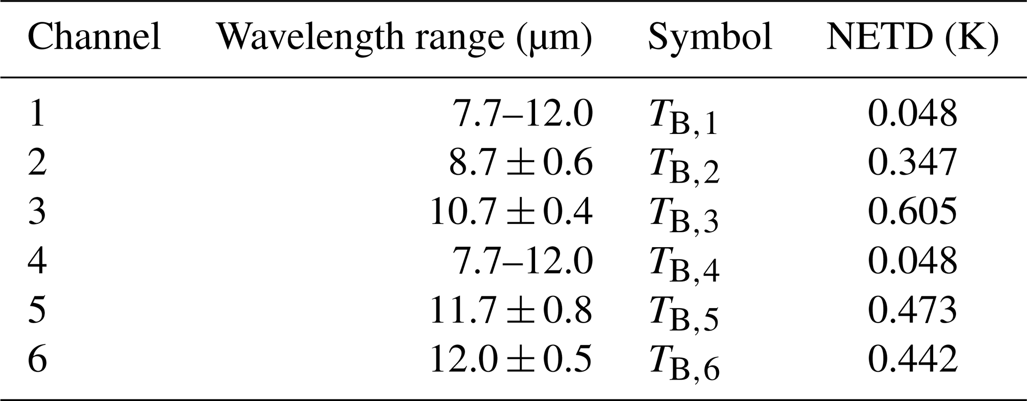
The instrument is operated with six spectral filters resulting in six channels, of which two are redundant broadband channels (channel 1 and 4). The remaining channels are narrow-band, each centred on specific wavelengths. The uncertainty in the measurements is characterized by the net equivalent temperature difference (NETD) for each channel. The broadband channels have a NETD of 0.048 K, while the narrow-band channels show varying NETD values shown in Table 1. For HALO–(𝒜𝒞)³, the corrected brightness temperature data, resampled to 1 s temporal resolution, were provided by Schäfer et al. (2023). To retrieve cloud cover, the HALO Microwave Package (Mech et al., 2014, HAMP) and the water vapour differential absorption lidar WALES (Wirth et al., 2009) were installed on HALO. In addition, 330 dropsondes (George et al., 2024) were released during the campaign. We have restricted our analysis to cloud-free scenes in the MIZ. For this purpose, a cloud mask based on campaign-specific radar reflectivity and lidar backscatter coefficient thresholds was applied (Konow et al., 2019). To ensure the data quality, each scene was visually examined to confirm the absence of clouds.

2.2 Satellite data

Independent measurements of surface skin temperature were provided by MODIS sea-ice surface temperature (IST;  Hall and Riggs, 2021) and sea surface temperature (SST;  NASA, 2024). Both datasets were based on a split-window retrieval algorithm, which determined surface skin temperature from the measured brightness temperatures. For the respective surface types, MODIS channels 1 (0.645 µm), 2 (0.865 µm), 4 (0.555 µm), 6 (1.64 µm), 31 (11 µm), and 32 (12 µm) were used. The IST dataset were provided as swaths with a horizontal resolution of 1 km by 1 km, while the SST dataset is gridded with a horizontal resolution of 4 km by 4 km. Daily fields of SIC were provided by the assimilated MODIS/AMSR-2 SIC product, derived from a synthesis from MODIS and AMSR-2 (Ludwig et al., 2019). Depending on the combination of MODIS and AMSR-2, the fields of SIC have a 5 km horizontal resolution for all conditions and 1 km for cloud-free scenes. Satellite images in terms of spectral radiance with high horizontal resolution were obtained from the Sentinel-2 multispectral imager (MSI, hereafter Sentinel-2) data. To characterize the surface reflectivity, the red (0.664 µm), green (0.559 µm), and blue (0.492 µm) (RGB) channels were sufficient, which have a horizontal resolution of 10 m by 10 m. For the high latitudes reached by HALO-(𝒜𝒞)³ observations, the revisit time of Sentinel-2 is about 1 d, which enabled daily observations and allowed for collocation of the satellite observations with VELOX images (Spoto et al., 2012). The Sentinel-2 data were accessed via the Google Earth Engine (GEE;  Gorelick et al., 2017).

3 Retrieval methods

3.1 Surface skin temperature

VELOX detects spectral radiances in the TIR wavelength range that are converted to TIR brightness temperatures, T_B, characterizing the combined emission by atmospheric components and the surface. Actually, a significant contribution results from emission by atmospheric gases, although the spectral bands are located in the atmospheric window region. This atmospheric contribution has to be removed from the signal to derive the surface temperature, also called surface skin temperature. To correct for the atmospheric emission between the aeroplane and the surface, a split-window method (SW) is commonly applied (McMillin and Crosby, 1984; Li et al., 2013). Adjusted to VELOX measurements, this approach can be formulated as follows:

$$\begin{array}{}\text{(1)}& T_{\mathrm{S}}=a_{\mathrm{sw}}+b_{\mathrm{sw}}\cdot T_{\mathrm{B},\mathrm{5}}+c_{\mathrm{sw}}\cdot (T_{\mathrm{B},\mathrm{5}}-T_{\mathrm{B},\mathrm{6}}).\end{array}$$

T_S represents the surface skin temperature, T_B,5 is the brightness temperature measured with VELOX channel 5 installed on HALO in about 10 km altitude, which is least affected by water vapour absorption. The coefficients a_sw, b_sw, and c_sw are empirically determined with a linear regression. Thus, $T_{\mathrm{B},\mathrm{5}}-T_{\mathrm{B},\mathrm{6}}$, represents the brightness temperature difference between channels 5 and 6, serving as a proxy for water vapour absorption. Vincent et al. (2008) found that this brightness temperature difference observed in the Arctic region is also sensitive to other parameters, such as atmospheric inversion height or aerosol particles. Their proposed single-channel algorithm (SCA;  Vincent, 2019) has been adapted to VELOX data as follows:

$$\begin{array}{}\text{(2)}& T_{\mathrm{S}}=a_{\mathrm{sca}}+b_{\mathrm{sca}}\cdot T_{\mathrm{B},\mathrm{5}}.\end{array}$$

We have performed radiative transfer simulations (RTSs) to constrain the contribution of atmospheric absorption to the surface skin temperature for both retrieval methods. The RTSs were conducted with the radiative transfer library (libRadtran;  Emde et al., 2016). The simulations were initialized with temperature and humidity profiles from dropsondes that were released from HALO during the campaign (Wendisch et al., 2024). The surface skin temperature was provided by MODIS (Hall and Riggs, 2021), whereas ozone content was given by the ERA5 reanalysis data (Hersbach et al., 2020).

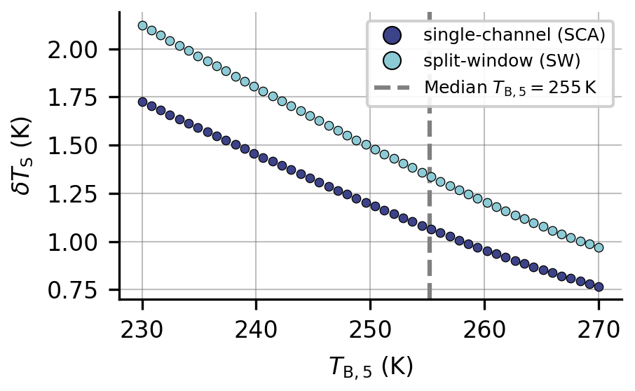
Figure 2 Empirically determined total uncertainty of the surface skin temperature retrieval δT_S as a function of VELOX-measured brightness temperature T_B,5. In dark blue, the total uncertainty was calculated for the SCA, in light blue for the SW.

For the molecular absorption parameters, REPTRAN medium (Gasteiger et al., 2014) was chosen, along with the DIScrete ORdinate Radiative Transfer solvers (DISORT;  Stamnes et al., 2000). To constrain the retrieval uncertainties as a function of the atmospheric total column water vapour concentration, the integrated water vapour (IWV) was varied from 0 to 50 kg m⁻². During the HALO–(𝒜𝒞)³ campaign, the integrated water vapour (IWV) was confined to values less than 10 kg m⁻² (Walbröl et al., 2024). To evaluate the two retrieval methods the total uncertainty δT_S was calculated for both algorithms. Adapted from Brown and Minnett (1999), who formulated the uncertainties for the MODIS IST retrieval, the total uncertainty of the VELOX retrievals was formulated as follows:

$$\begin{array}{}\text{(3)}& {\displaystyle }\mathit{\delta }{T}_{\mathrm{S}}^{\mathrm{sw}}=\sqrt{(\mathit{\delta }{T}_{\mathrm{atm}}^{\mathrm{sw}}{)}^{\mathrm{2}}+(\mathit{\delta }{T}_{\mathrm{VEL},i}{)}^{\mathrm{2}}},\text{(4)}& {\displaystyle }\mathit{\delta }{T}_{\mathrm{S}}^{\mathrm{sca}}=\sqrt{(\mathit{\delta }{T}_{\mathrm{atm}}^{\mathrm{sca}}{)}^{\mathrm{2}}+(\mathit{\delta }{T}_{\mathrm{VEL},\mathrm{5}}{)}^{\mathrm{2}}},\text{(5)}& {\displaystyle }\mathit{\delta }{T}_{\mathrm{vel},i}=\sqrt{(\mathit{\delta }{T}_{\mathrm{vel},i}^{\mathrm{sys}}{)}^{\mathrm{2}}+(\mathit{\delta }{T}_{\mathrm{VEL},i}^{\mathrm{ran}}{)}^{\mathrm{2}}},\end{array}$$

where

$$\begin{array}{}\text{(6)}& {\displaystyle }\mathit{\delta }{T}_{\mathrm{VEL},i}^{\mathrm{sys}}=A+B\cdot T_{\mathrm{B},i},\text{(7)}& {\displaystyle }\mathit{\delta }{T}_{\mathrm{VEL},i}^{\mathrm{ran}}={\mathrm{NETD}}_{\mathrm{B},i}.\end{array}$$

The overall uncertainty of the surface skin temperature δT_S was quantified as the square root of the sum of the squared uncertainties from the atmospheric correction and the uncertainty introduced by VELOX δT_VEL,i, which was split into a random part $\mathit{\delta }{T}_{\mathrm{VEL},i}^{\mathrm{ran}}$ equivalent to the NETD and a systematic part $\mathit{\delta }{T}_{\mathrm{VEL},i}^{\mathrm{sys}}$. The systematic uncertainty was parameterized based on the measured brightness temperature T_B,i in channel i. The superscripts “sca” and “sw” correspond to the respective algorithms, while the index subscript i indicates VELOX channel i. The total uncertainty for both retrievals, depending on T_B,5 and assuming a constant δT_atm, is shown in Fig. 2. Due to the difference in considering only the NETD of channel 5 for the SCA and both NETDs of channel 5 and 6 for the SW, the SCA retrieval has a lower error across all temperature ranges.

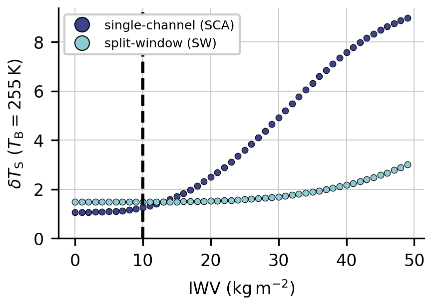
Figure 3 Comparison of surface temperature retrieval uncertainty (δT_S) as a function of integrated water vapour (IWV, kg m⁻²) for the single-channel algorithm (dark blue) and split-window method (light blue).

To evaluate the sensitivity of the retrievals to IWV, the total uncertainty of both retrievals as a function of IWV is shown in Fig. 3. Below the IWV threshold of 10 kg m⁻², the SCA outperforms the SW, due to the reduced NETD only using one channel. Above this threshold, atmospheric absorption dominates the total uncertainty favouring the SW algorithm. In summary, the single-channel algorithm has a lower total uncertainty for IWV values below 10 kg m⁻², while the split-window algorithm is more suitable for more humid atmospheres. Therefore, the SCA is applicable in the Arctic region when low IWV concentrations are present.

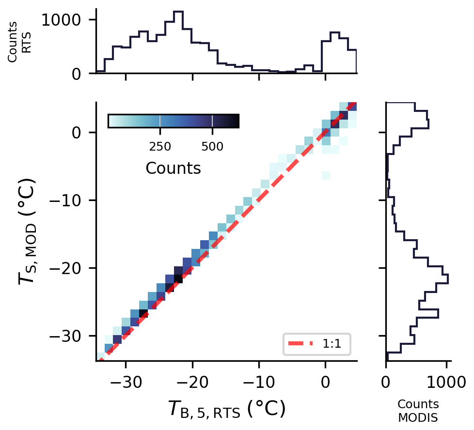
Figure 4 MODIS skin temperature T_S,MOD is compared to the simulated brightness temperature at HALO flight altitude for VELOX channel 5 (11.5 µm) T_RTS,B5.

As a consequence, we continue with the derivation of the regression coefficients a_sc,b_sc of the SCA algorithm. For this purpose, the RTSs were performed with a temporal resolution of 1 s, resulting in simulated brightness temperature values for VELOX channel 5 $T_{\mathrm{B},\mathrm{5},\mathrm{RTS}}$ at HALO flight altitude. These simulated brightness temperature values at flight altitude are linearly regressed against MODIS surface skin temperature. The resulting fit parameters for slope and offset serve as the single-channel coefficients:

$$\begin{array}{}\text{(8)}& {\displaystyle }{a}_{\mathrm{sc}}=\mathrm{9.051}\mathrm{K}\text{(9)}& {\displaystyle }{b}_{\mathrm{sc}}=\mathrm{0.967}{\mathrm{K}}^{-\mathrm{1}}.\end{array}$$

In Fig. 4, MODIS surface skin temperatures T_S,MOD were plotted against simulated brightness temperature $T_{\mathrm{B},\mathrm{5},\mathrm{RTS}}$. The regression shows a coefficient of determination of R²=0.99 and a root mean square error (RMSE) of 0.47 K. Substituting ${\mathit{\delta }}_{\mathrm{atm}}^{\mathrm{sc}}=\mathrm{0.47}$ and NETD=0.473 K into Eq. (4), the overall uncertainty of the SCA algorithm using RTSs with ERA5 IWV data was computed as

$$\begin{array}{}\text{(10)}& \mathit{\delta }{T}_{\mathrm{S}}=\mathrm{1.1}\pm \mathrm{0.3}\mathrm{K},\end{array}$$

where the range of δT_S reflects the error for different measurement conditions.

3.2 Surface type classification

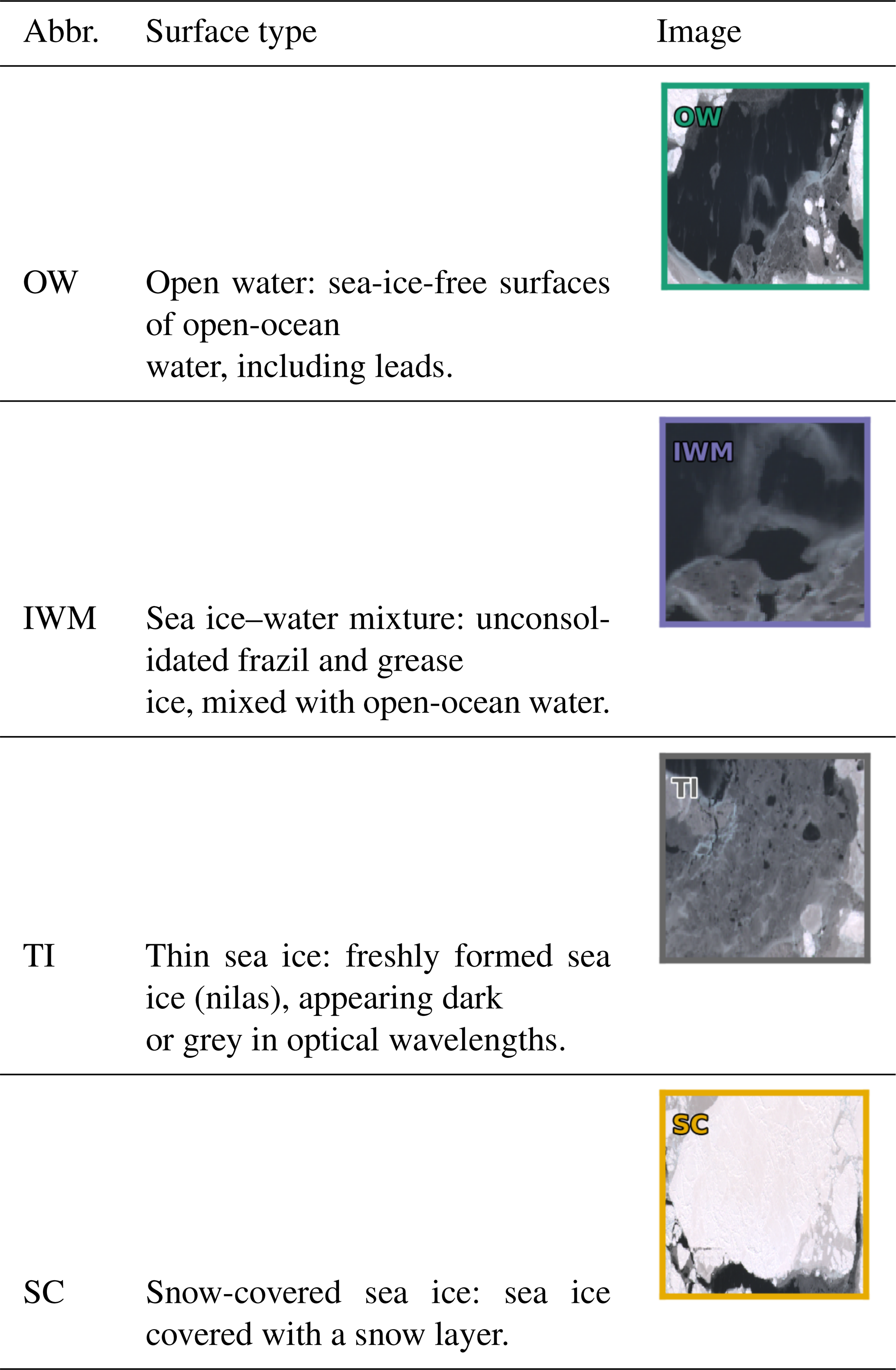
To distinguish different surface types, we have adapted established definitions (Miao et al., 2015; Wright and Polashenski, 2018; Jäkel et al., 2019a). As no melt ponds were observed during HALO-(𝒜𝒞)³, this surface type was omitted. To illustrate the surface types, a Sentinel-2 true colour image is analysed in Fig. 5. All surface types applied in this study are present in this scene and characterized in Table 2.

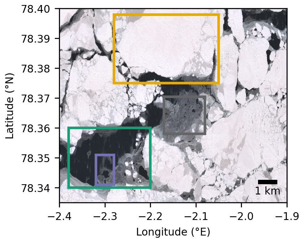
Figure 5 True colour image provided by Sentinel-2 on 4 April 2022 at 13:35:00 local time. The four coloured rectangles represent the surface types selected for this study: sea-ice-free open water (green), ice–water mix (purple), thin sea ice (grey), and snow-covered sea ice (yellow).

Table 2 Surface types with short characterization, corresponding abbreviations, and representative images from Fig. 5.

The image analysis consists of three steps. First, the VELOX 2D-images are preprocessed. Next, a random forest (RFA) classification algorithm is applied for pixel-wise surface classification. Finally, a segmentation algorithm is used to identify and summarize areas of the same surface type.

3.2.1 Preprocessing images

Since the temporal sampling rate of the VELOX data was 1 Hz, and the typical cruise speed of HALO was about 200 m s⁻¹, it was possible to construct push-broom-like images (PLIs) of the corresponding nadir strips at each time step. With this technique, the effect of the viewing zenith angle (VZA) on the measured brightness temperature can be neglected. Furthermore, georeferencing was performed for each data point of the PLI, providing crucial information about the geographic location of the measurement. This process incorporates the geographical position, flight altitude, and attitude data from HALO, as well as the calculated viewing azimuth and zenith angles for the applied lens and detector combination of VELOX and the measured mounting direction of VELOX.

3.2.2 Random forest classification of surface types

To determine the surface type, a random forest (RFA) was implemented in a pixel-by-pixel fashion; i.e. each pixel was individually classified. The RFA comprises a supervised machine learning method that constructs ensembles of decision trees, which are fitted to user-defined ground-truth data. It combines the interpretability of decision trees with the robustness to noise characteristics of other ensemble methods (Breiman, 2017; James et al., 2023). For the implementation of the RFA, the machine learning library autogluon (Erickson et al., 2020) was used, allowing for a comparison of multiple machine learning methods. Compared to other supervised learning algorithms, the RFA demonstrated comparable accuracy, while significantly reducing computation time.

Table 3 Input parameters as processed from VELOX measurements and used in the pixel-wise RF surface type classification.

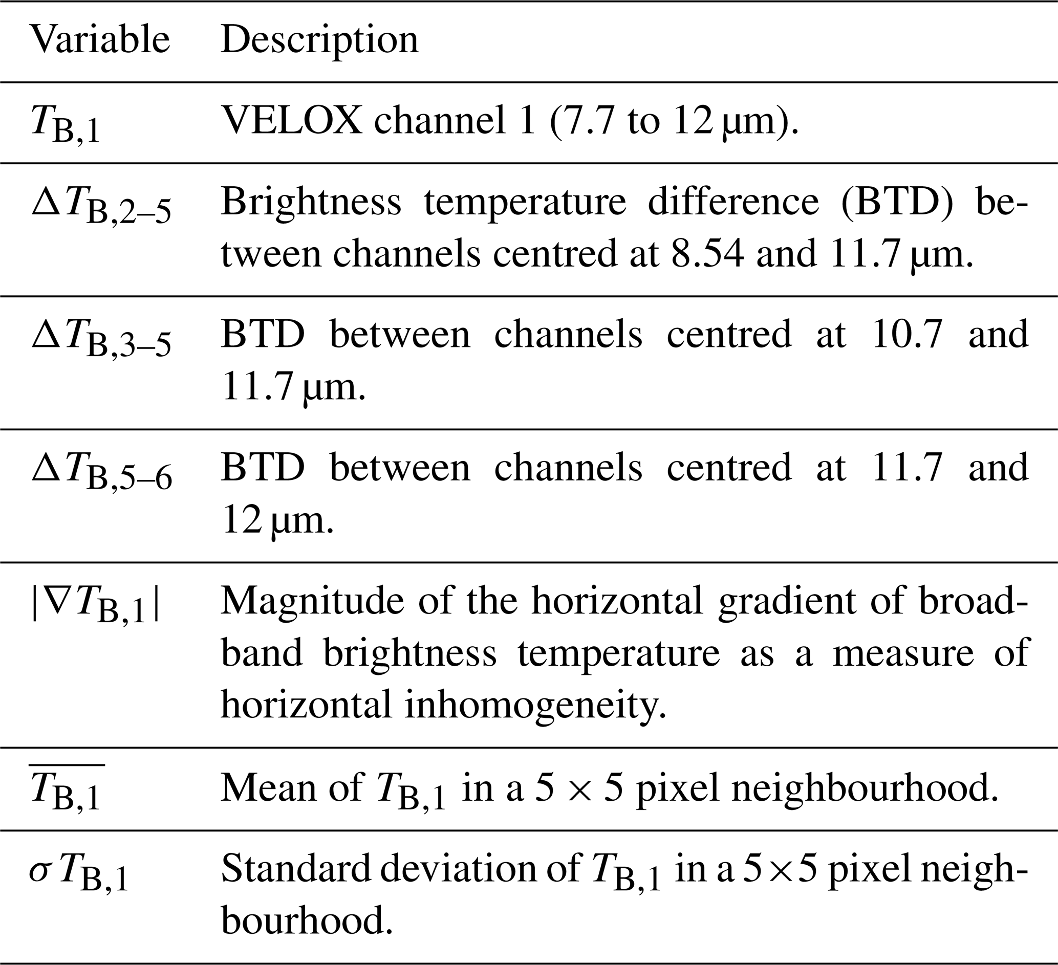
Sentinel-2 images classified manually were used as the ground truth. For labelling these images, the Computer Vision Annotation Tool (Sekachev et al., 2020, CVAT) was applied. In total, 58 VELOX images from 10 research flights were labelled, resulting in 13 million labelled pixels. The locations of the training data are depicted as pink stars in Fig. 1. The training data were sampled randomly from the available data (Sentinel-2 image available, cloud free) and subsequently filtered to resemble all latitudes equally. Seven input features, as defined in Table 3, are applied to the RFA. All parameters are calculated from VELOX brightness temperature data.

The accuracy of a multi-class classification problem can be expressed by the ratio of correct to all predictions. When validated in a 5-fold cross-validation setup, the RF showed an accuracy of 87 % with respect to the test data.

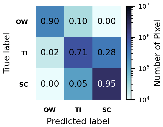
Figure 6 Confusion matrix of the RFA prediction, showing the percentage of the correctly predicted pixels on the diagonal. The off-diagonal elements represent the false positive and false negative values.

To further assess the performance of the RFA, a confusion matrix is shown in Fig. 6. The highest accuracy is achieved on the SC surface type (95 %), followed by the OW surface type (90 %). The TI surface type achieves a lower overall accuracy with 71 %, due to transitional nature of this surface type. In Fig. 7b, the initial RFA classification for an example scene is shown. A common challenge when using RFA for image classification is the speckles, as seen in this figure. To address this issue, segmentation is required, which is described in the next section.

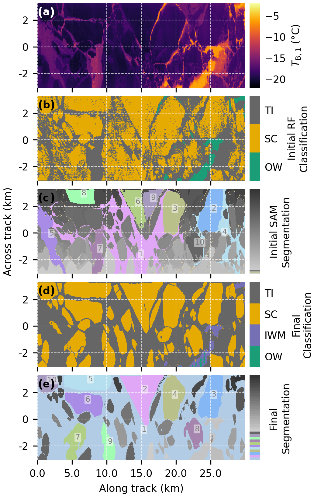
Figure 7 Overview of surface classification and segmentation results for the push-broom-like image captured on 4 April 2022 from 13:36:14 to 13:38:31 UTC. (a) Broadband brightness temperature T_B,1 (7.7–12 µm) as push-broom-like image. (b) Initial surface type classification using the random forest algorithm (RFA), identifying open water, thin ice, and snow-covered ice. (c) Initial segmentation using the segment-anything model (SAM), with numbered segments representing the 10 largest areas for illustration. (d) Final surface type classification: the most common surface type within each segment from (c) was assigned, and a surface skin temperature threshold was used to sort the ice–water mix (IWM) from OW. (e) Final segmentation, where new segments were assigned to all connected regions of the same surface type derived from (d), with the largest segments again highlighted by their respective numbers.

3.2.3 Segmentation

To assign the predefined surface types to the retrieved fields of surface skin temperature, the PLIs are subjected to the open-source image segmentation algorithm segment-anything (SAM; Kirillov et al., 2023). The SAM algorithm image segments on the basis of colour gradients and points that are placed by the user. The initial segmentation of an exemplary scene is shown in Fig. 7c. Although the model was not fine-tuned, i.e. not trained with a specific user dataset, it proves a high capability to segment previously unseen data in a zero-shot fashion (Wu and Osco, 2023; Ren et al., 2024). This offers an advantage over training a segmentation algorithm, which is demanding in terms of data points and computational time.

To automatically generate a segmentation mask with SAM, a grid of points is placed on the PLI and then recursively shifted to avoid over-segmentation of the images. This means that initially a grid is constructed on the image, and the algorithm searches for segments close to the grid points. To ensure stable segmentation, the grid is divided into smaller subgrids, which are then shifted relative to the initial grid points. This process is repeated three times. Since some over-segmentation still occurs, resulting in smaller predicted segments than those identified by humans, information from surface classification is added to the segmentation. First, each segment identified by SAM is subjected to a majority vote, meaning the most frequently occurring surface type within a particular segment is assigned to that segment. Finally, the segments are obtained by merging neighbouring segments of the same surface class. This results in a natural image segmentation, which is illustrated in the lowest panel of Fig. 7e.

This merging step can connect large, contiguous areas of a single surface type (e.g. thin ice), which can influence feature size statistics. Therefore, the initial, finer-grained segmentation from SAM (prior to merging) is retained for a sensitivity analysis (see Sect. 4.3). To allow for full transparency and further exploration by the community, both the initial and final merged segmentation masks were provided in our public dataset (Müller et al., 2025). In a final post-processing step, the IWM class is identified to ensure the physical consistency of the final product. This step addresses instances where pixels were classified as OW despite having temperatures well below the physical freezing point of seawater. Specifically, any OW pixel with a surface skin temperature cooler than −3 °C was reclassified as IWM. This threshold was chosen to represent a sub-pixel sea-ice fraction of greater than 33 %, assuming the sub-pixel surface skin temperature of sea ice to be −15 °C and the surface skin temperature of OW close to the freezing point of −1.7 °C (Skogseth et al., 2009; De La Rosa et al., 2011).

4 Results and discussion

4.1 Surface skin temperature

In Fig. 8, the VELOX-retrieved surface skin temperature T_S,VELOX is compared to the MODIS surface skin temperature T_S,MOD, obtained from Hall and Riggs (2021) and NASA (2024), showing the coefficient of determination R² to be equal to 0.96.

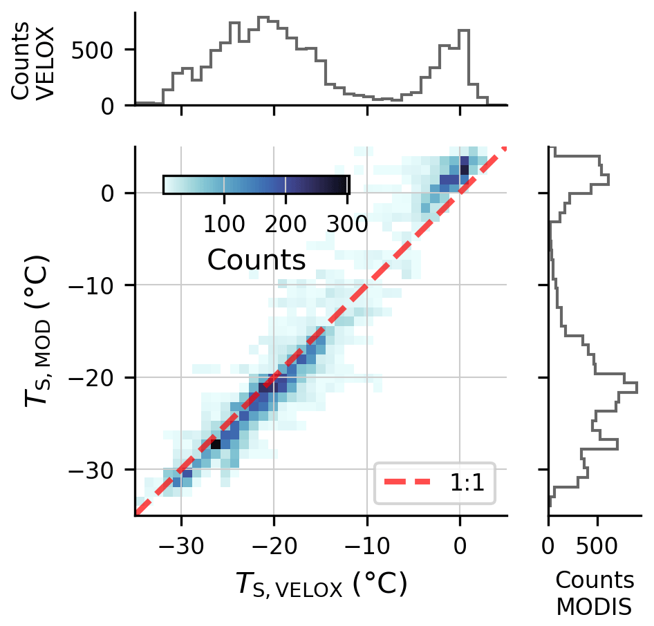
Figure 8 Scatter plot of MODIS T_S,MOD against VELOX-retrieved T_S,VEL, with VELOX data averaged to match the MODIS pixel size. The appended frequency distributions show the corresponding surface skin temperature distributions for both datasets.

For this comparison, the instantaneous FOVs of the single VELOX pixels were combined by averaging to fit the MODIS pixel-size, allowing for a direct comparison between their two datasets. The RMSE was determined to be 2.0 K with a bias of 0.51 K and a mean average difference of 1.55 K. Furthermore, Fig. 8 indicates slightly higher values of surface skin temperature derived from VELOX, T_S,VELOX, with respect to MODIS, T_S,MOD, over sea ice and lower values over open water. As the dataset comprises multiple days, it is essential to provide information on the location of the data. To simplify this spatial information into a scalar, the data are grouped by their distance to the sea-ice edge (positive direction into the internal ice zone). As the individual pixels have been georeferenced, their relative distance to the nearest sea-ice edge (defined by campaign-averaged SIC values between 9 %–11 %) is computed. For this, the distance of each spatial segment centre to the temporally closest available AMSR-2/MODIS SIC pixel is calculated. The mean surface skin temperature coloured by surface types is plotted in Fig. 9a against the distance to the sea-ice edge.

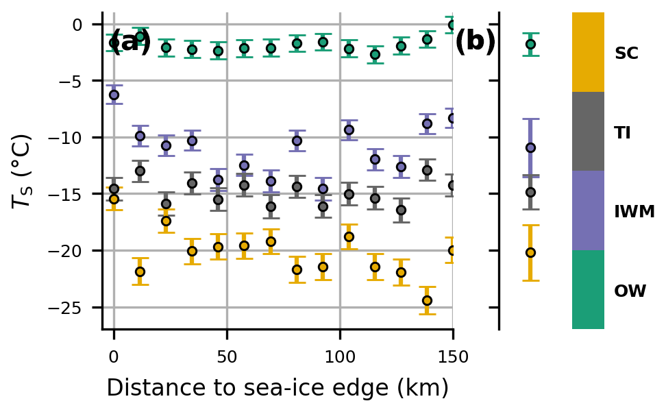
Figure 9 (a) Mean T_S of different surface type segments, weighted by segment size and aggregated over 10 km bins from the sea-ice edge into the internal ice zone. (b) Mean T_S over all marginal sea-ice-zone segments.

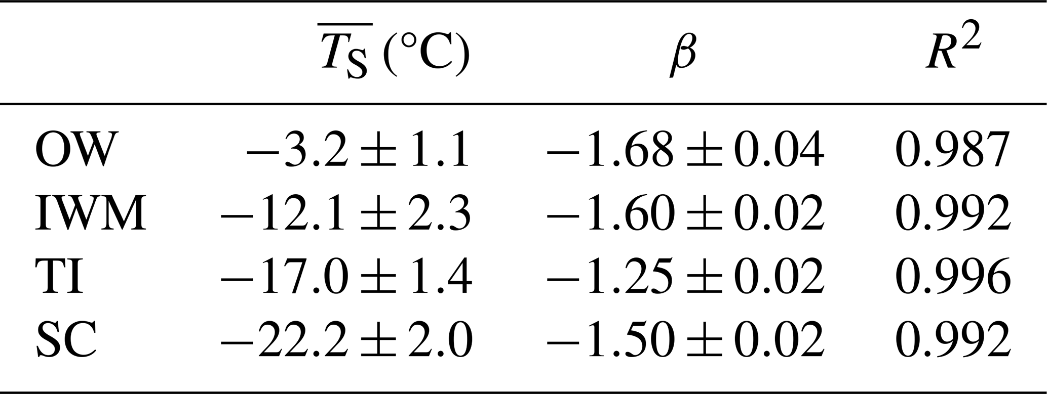
In Fig. 9b, the mean surface skin temperature of all segments $\stackrel{\mathrm{‾}}{T_{\mathrm{S}}}$, weighted by their size, is shown. A clear separation between the $\stackrel{\mathrm{‾}}{T_{\mathrm{S}}}$ of different surface types is observed as expected. The values from Fig. 9b are displayed together with the corresponding error range in Table 4.

4.2 Spatial analysis of surface types

From the segmentation, we retrieve the corresponding segment size, mean temperature, and standard deviation of each segment. The results are illustrated in Fig. 10, showing the spatial distance of each segment centre to the nearest sea-ice edge plotted against the corresponding surface type. The fraction of the open-water surface type decreases from 40 % to below 5 % in the first 20 km, while the fraction of the snow-covered surface type becomes increasingly dominant when approaching the pack ice. The surface types thin ice and ice–water mix maintain relatively constant fractions of occurrence across all considered distances from the ice edge, with no clear trend observed.

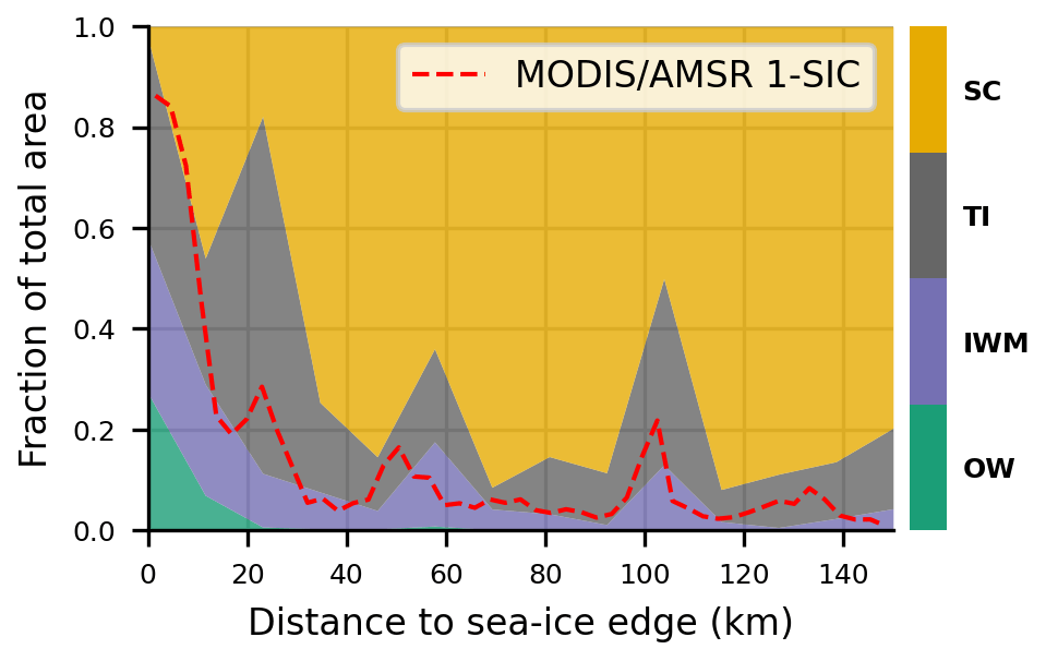
Figure 10 Fraction of total area for the four surface classes as a function of the distance to the closest sea-ice edge. The red dashed line indicates the open-water fraction (1.0 - SIC) from MODIS/AMSR-2 (Ludwig et al., 2019).

When compared with the provided SIC from MODIS/AMSR-2, the computed RMSE and mean absolute difference (MAD) are 8 % and 5 %, respectively. For this comparison, the nearest available SIC data from the satellite product were matched with a similar FOV of the VELOX PLI. The errors result from the temporal mismatch between both datasets, as MODIS/AMSR-2 SIC is only available as a daily gridded product. When comparing the bias, i.e. the difference between VELOX SIC and MODIS/AMSR-2 SIC, an underestimation of 3 % or an overestimation of 5 % is observed, depending on whether only pixels classified as open water are considered open water or if pixels classified as both open water and ice–water mix are included. As shown in Fig. 10, the open-water fraction and the area fractions derived from VELOX agree within the given error range.

4.3 Segment size distribution

Since the segmentation enables the measurement of individual segment sizes, an analysis of the spatial structure of the data is performed. Here, we extend the concept of the floe size distribution (FSD; Rothrock and Thorndike, 1984; Herman, 2010; Bateson et al., 2022) to the segment size distribution N_SSD, resulting in the following description:

$$\begin{array}{}\text{(11)}& N_{\mathrm{SSD}}\left(x_{\mathrm{SEG}}\right)=C\cdot (x_{\mathrm{SEG}}{)}^{\mathit{\beta }}.\end{array}$$

Here, x_SEG represents the segment size in units of m², C is an empirical constant, and β is the dimensionless power-law exponent describing the scaling of the distribution. The closer the exponent is to zero, the more N_SSD favours large segments. This approach simplifies the complex spatial heterogeneity of the MIZ by expressing the scaling of N_SSD using β, a single scalar value.

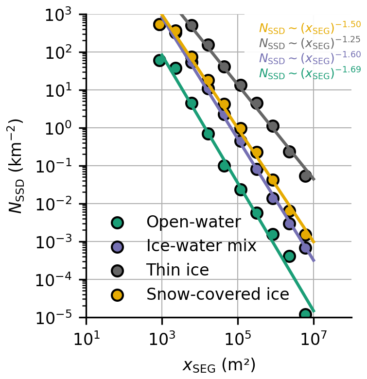
Figure 11 Double-logarithmic graph of the segment size density (coloured dots) for all four surface types as a function of the segment size. The surface types are colour-coded, indicating open water (green), ice–water mix (purple), thin ice (grey), and snow-covered ice (yellow). Linear fits (coloured lines) are added in the respective surface type colour, providing the exponents listed in the top right.

In Fig. 11, the segment size density N_SSD (in units of km⁻²) for different surface types is displayed in a double-logarithmic graph as a function of the segment size, x_SEG. In addition, the individual distributions are fitted with a linear model. The slope of each linear fit corresponds to the exponent of the power-law distribution, β. The different β_i values computed for each surface type are shown in Table 4.

Table 4 Summary of mean surface temperature $\stackrel{\mathrm{‾}}{T_{\mathrm{S}}}$, power-law exponents β, and goodness of fit R² for the corresponding N_SSD, for different surface types.

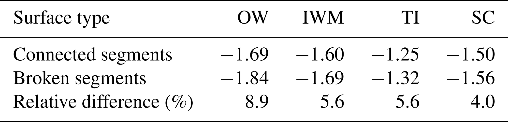
We conclude that, in addition to the different sea-ice types, the surface types ice–water mix and open water also follow a power-law distribution. The computed β values for, for example, the snow-covered sea-ice type are in the range of corresponding literature data, with values ranging from −0.91 to −2.9 (Herman, 2010). A key characteristic observed during our flights over the MIZ was the presence of large, contiguous areas of thin ice or snow-covered ice, which can appear as very large segments in our final classification (e.g. Fig. 7e). We interpret these as genuine physical features of newly forming ice in the MIZ at the time of observation rather than as segmentation artefacts. However, we acknowledge that the definition of a “segment” is sensitive to the processing methodology and that the scale of these large features can influence the resulting feature size distribution (FSD). To quantify this sensitivity, we performed an additional analysis by calculating the FSD statistics on the initial, finer-grained segmentation generated by SAM, before our final step of merging adjacent segments of the same class (an example of this initial stage is shown in Fig. 7c). The results, summarized in Table 5, demonstrate that the power-law coefficients change by 4 % to 8 %, depending on the surface type.

Table 5 Power-law coefficients for the four surface types, with “Connected segments” denoting the final segmentation where same surface type segments are merged and “Broken segments” the finer SAM segmentation.

To gain more insight into the spatial heterogeneity within the MIZ, we fit the N_SSD of the snow-covered segments to 10 km sized bins of distance to the sea-ice edge (in pack-ice direction).

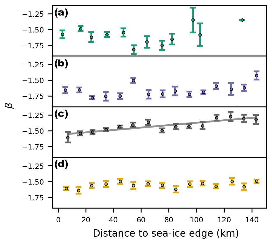
Figure 12 Power-law exponent β of the segment size distribution N_SSD, binned in 10 km steps, starting from the sea-ice edge into the direction of the internal ice zone by surface type. For (a) open water, (b) ice–water mix, and (d) snow-covered ice, no trend is observed. For (c) thin ice, a significant linear trend is observed.

In Fig. 12, the size power-law exponent β is shown as a function of the distance to the sea-ice edge for the different surface types. A linear trend is fitted only to the TI data, suggesting significance with a R²=0.76 and a p value less than 0.001. The increase in β from −1.6 to −1.3 reflects a physical characteristic of the MIZ. Closer to the sea-ice edge, a higher number of smaller segments is observed (more negative β) due to intensified floe breakup, whereas larger floes (less negative β) become more prevalent further into the MIZ, where ocean wave propagation is more attenuated (Herman, 2010; Denton and Timmermans, 2022).

5 Summary and conclusions

During the HALO–(𝒜𝒞)³ aircraft field campaign, covering the Fram Strait to the North Pole in March and April 2022, an extensive dataset of surface and atmospheric properties was measured by a variety of instruments mounted on three research aircraft (Wendisch et al., 2024). The data were compiled by the High Altitude and LOng range research aircraft (HALO), which was instrumented with radar, lidar, a dropsonde launching facility, microwave radiometer, and various spectral imagers (Ehrlich et al., 2025). This study was based on observations collected by the VELOX (Video airbornE Longwave Observations within siX channels;  Schäfer et al., 2022) thermal infrared (TIR) imaging system, which was installed on HALO in a nadir viewing direction. Due to its fast-spinning filter wheel (100 Hz) equipped with multiple spectral band-pass and long-pass filters, a high spatial resolution of 10 m by 10 m pixel size for a target at 10 km distance is achieved with VELOX, providing valuable high-resolution TIR spectral radiances expressed in brightness temperatures.

Using VELOX data from HALO–(𝒜𝒞)³, which are publicly available from Schäfer et al. (2023), a single-channel (SCA) surface skin temperature retrieval based on linear coefficients derived from radiative transfer simulations (RTSs) was adapted. Comparisons with multiple-channel retrievals and surface skin temperature products from the MODerate resolution Imaging Spectroradiometer (MODIS;  Hall et al., 2004; Hall and Riggs, 2021; NASA, 2024) provided agreement in the range of 2 K, with a coefficient of determination of R²=0.96 and a bias of 0.5 K. To categorize the obtained surface skin temperature fields, a surface type classification algorithm was developed based on publicly available software tools combined with physically reasonable thresholds applied to regenerated push-broom images from the initial brightness temperature data. The resulting two-dimensional fields provide segment-vise information of the surface type, which can then be analysed in combination with, e.g. the retrieved surface skin temperature. The data were classified into the following surface types: open water (OW), thin ice (TI), ice–water mix (IWM), and snow-covered ice (SC). The IWM class was identified in a post-processing step, reclassifying all OW pixels with a surface skin temperature of less than −3 °C as IWM.

With the surface skin temperature and surface classification retrievals, important parameters were obtained with high spatial resolution. When computing the resulting sea-ice concentration (SIC) from the surface classification, agreement with a bias of about 5 % with the MODIS/AMSR-2 product was obtained, if the IWM surface type is assigned to be “sea-ice-free”. Additional sensitivity studies will be required to assess the influence of this surface type. The established classification serves as a promising foundation for these future investigations. The retrieved power-law segment size statistics are generally consistent with values reported in the literature (Denton and Timmermans, 2022). For the snow-covered surface type, these findings align with those of Herman (2010), who observed power-law exponents ranging from −0.91 to −2.9 and reported an increase in the exponent when transitioning from the sea-ice edge to the interior ice zone. Overall, although the temporal duration and the spatial extent of the presented dataset are limited, agreement with other studies emphasizes its value for the sea-ice community. Extending this analysis to different seasons will be crucial for capturing processes like melt pond evolution, though this will require multi-sensor data fusion to resolve the increased complexity of surface types. Therefore, the primary value of this high-resolution methodology lies in providing “ground truth” for calibrating satellite retrievals and refining sub-grid-scale parameterizations in pan-Arctic models.