Comparison of the performance between three Doppler wind lidars and a novel wind speed correction algorithm

Doppler wind Lidars (DWLs) have been widely used to detect wind vector variations, based on ground monitoring of atmospheric boundary layer and wind shear. This study evaluates the performance between three DWLs and in situ balloon radiosonde. Lidars data comparison focuses on low altitudes (height <2 km) from July to September 2021 from three producers: MSD (Minshida), CUIT (homemade), and WP (windprofile) Lidars. Within the research height range, comparisons show the root mean square errors (RMSE) for wind speed were 1.11, 4.45, and 5.15 m s⁻¹, while wind direction RMSE were shown at 49.83, 82.89, and 84.87°, respectively. The measurement accuracy decreases with the altitude increase (up to 2 km). The Lidar performance requires a certain amount of aerosol backscattering, when PM_2.5 ranges within 35–50 µg m⁻³, MSD Lidar exhibited the highest wind speed correlation (R²=0.82) with radiosonde, and the wind direction accuracy observed with the three Lidars is enhanced with the increase of aerosol concentration, indicating that particle loading is the critical factor affecting the wind profile. Lidar performance varied significantly with planetary boundary layer heights (PBLH), particularly, the Lidar performance is relatively optimal when the PBLH within 500–750 m, with the Pearson correlation coefficients (PCCs) of wind speed are 0.97, 0.92, and 0.72, while the wind direction is shown at 0.98, 0.75, and 0.70, respectively. The vertical relationship between cloud base height (CBH) and PBLH had also varied influences on the Lidar measurements. Machine learning was used to remove anomalies and complement missing values, the random forest (RF) demonstrated superior performance, with the Area Under the Curve (AUC) of 0.93(CUIT) and 0.90(WP) in the Receiver Operating Characteristic (ROC) curves. RF-based correction of CUIT data enhanced the R² from 0.42 to 0.65. The R² between the RF-based CUIT and Aeolus satellite data was 0.83, indicating that the method effectively improved data, even in circumstances of anomalies. We proposed a new correction algorithm combined with the isolation forest (IF) and RF to handle high-dimensional and incomplete datasets. Our procedure could increase the Lidar measurement quality of wind.

1 Introduction

The development of the low-altitude economy depends on efficient airspace management and flight scheduling. The Lidar technology has laid a strong foundation for turbulence measurement, wind shear detection, gravity wave analysis, and boundary layer height estimation (Chanin et al., 1989; Harvey et al., 2015; Sathe and Mann, 2013; Shun and Chan, 2008; Talianu et al., 2006). The biggest, most significant risk of unmanned aerial vehicle (UAV) flight is the wind shear in the low layer at the boundary. DWL uses the optical Doppler effect to measure atmospheric wind speed by detecting the frequency shift between emitted and backscattered laser signals, offering high spatial and temporal resolution measurements (Du et al., 2017).

Conventional wind measurement systems face inherent limitations. In recent years, Lidar has successfully overcome many of the limitations associated with conventional detection equipment (Liu et al., 2019). For example, differing from mechanical anemometers, DWL can remotely measure wind speed without contact with the atmosphere (Tavakol Sadrabadi and Innocente, 2024). Radiosondes, reckoned as the best accuracy, suffer from discontinuous temporal sampling and cannot support all-weather monitoring (Abdunabiev et al., 2024). In observational experiments, there are phenomena leading to anomalies and missing DWL data. These errors may arise from different atmospheric conditions, for instance, the strong aerosol concentration and Brillouin backscattering signals may lead to errors in retrieving low-altitude wind speeds (Fahua et al., 2021). Traditional Lidar data inversion methods (e.g., Velocity Azimuth Display, VAD; Doppler Beam Swinging, DBS) exhibit horizontal wind speed errors exceeding 10 % in complex terrains (Liu et al., 2022). Differences in pulsed laser instruments can affect the detection efficiency and accuracy of Lidar's detection (Ge et al., 2014), as well as data processing methods (Smalikho and Banakh, 2016).

Machine learning has been demonstrated to have the ability to solve missing values and improve DWL accuracy, such as noise filtering and data imputation (Lin et al., 2022; Lolli, 2023; Yang et al., 2021). Meteorological data have the characteristics of time series, and machine learning methodologies such as the RF and neural networks have been proved effective in unveiling latent patterns in wind-related time series data. The incorporation of machine learning-based validation and quality control algorithms has the potential to enhance wind measurement accuracy and facilitate the prediction of upper-level wind fields. In recent years, wind field data has received a lot of attention, and the RF algorithms are particularly popular (Vassallo et al., 2020; Wang et al., 2017). For example, the RF algorithm has been used to correct numerical model wind predictions for weather forecasting (Wang et al., 2021), improving forecast accuracy significantly. The RF algorithm employs an ensemble of decision trees to mitigate overfitting and enhance prediction robustness (Hastie et al., 2009). It has been proved to enhance prediction accuracy without a substantial increase in computational cost, to be robust against multicollinearity, and to demonstrate considerable stability in scenarios involving anomalies (Boulesteix et al., 2011). The RF algorithm has been demonstrated to address missing data effectively and to manage high variability, rendering it well-suited for the preprocessing of wind datasets (Zhao et al., 2024b). In comparison to other algorithms, such as AdaBoost and K-nearest neighbors (KNN), RF demonstrates superior performance in predicting wind speed and power generation, as evidenced by reduced mean absolute percentage error (MAPE) values (Malakouti, 2023). This study proposes the RF algorithm for Lidar wind data to develop a wind profile correction algorithm. For the verification of wind profiles, a radiosonde will be used to enhance the stability of the system and evaluate the feasibility of the algorithm (Huang et al., 2021).

Spaceborne wind Lidar technology is also effective for wind detection (Kim et al., 2021). Satellite retrieval for wind field information has become an important trend for future applications. The combination of ground-based and spaceborne Lidar enables high-precision atmospheric wind speed observation, which is crucial for weather forecast and wind energy development, but data acquisition rates for lower atmospheric layers significantly decrease under multilayered clouds or optically thick cloud systems (Belova et al., 2021; Rennie et al., 2021). Satellites equipped with scatterometers and radiometers, such as Metop-A, Metop-B, and Coriolis (He et al., 2022a; Silva et al., 2022), provide wind speed and direction. The Aeolus satellite, launched by the European Space Agency in 2018, is the first to provide comprehensive global wind observation. It operates in a 320 km sun-synchronous orbit, following a flight path roughly along the Earth's day-night boundary, and completing one orbit every 90 min (Belova et al., 2021). The satellite provides high-quality wind components and aerosol optical properties from the Earth's surface to the lower stratosphere (Belova et al., 2021; Flament et al., 2021). The satellite with a 1.5 m diameter Lidar system emits ultraviolet laser pulses and collects scattered light particles from the atmosphere at altitudes of 20–30 km. Wind speed, direction, and other parameters are determined by measuring the Doppler shift of the light waves (Witschas et al., 2020). This technology is one of the most effective measurements. In 2021, Guo et al. (2021) compared data from the European Space Agency's satellite with domestic wind profiler RWP network measurements, finding a good match between the Aeolus wind product and the RWP data. Chen et al. (2021) examined the seasonal variation in Aeolus satellite detection performance in China by combining ERA5 and radiosonde data, concluding that the satellite's performance is influenced by seasonal factors. Mie winds exhibit minimal systematic bias in regions with strong scatterers (typically clouds/aerosols), though random errors vary with signal strength. Rayleigh winds show small biases and random errors in the clear-sky free troposphere but face increased uncertainty in cloud-affected regions or the clear-sky boundary layer. Within cloud layers, Rayleigh channel signals are heavily scattered and absorbed by cloud particles, necessitating reliance on the Mie channel. Aeolus' strength lies in its global coverage, whereas its weaknesses include vertical resolution, cloud-penetration capability, and high sensitivity to clouds. Radiosondes remain an unparalleled reference benchmark, especially for validating Aeolus under cloudy conditions-despite their spatial representativity limitations. However, there is still a gap between comparing and validating Aeolus satellite products and Lidar data. Joint comparisons of spaceborne and ground-based measurements are essential for assessing the advantages and limitations of Lidar in accurately capturing wind fields, which will support the integration of laser sensors and inversion algorithms in next-generation wind measurement satellites.

This study investigates wind field measurements using three ground-based Doppler Lidar systems (CUIT, MSD, and WP Lidars) through a three-month comparative campaign at the Nanjiao Observatory in Beijing, collocated with radiosonde observations. the accuracy of the three ground-based Lidars are evaluated against radiosonde data as the reference standard. The study investigates the impact of PM_2.5 concentration on wind measurement performance. The effect of height on wind speed and direction was analyzed by comparing the Lidar performance under different PBLH and CBH conditions. The study also conducts satellite-ground validation to assess the consistency of the Aeolus Satellite. We propose a novel machine learning framework for wind profile correction by comparing various algorithms to optimize the data accuracy.

2 Instruments and methods

2.1 Method and instruments

The experiment was conducted at Beijing's Nanjiao Observatory (39.80° N, 116.32° E, 30 m a.s.l.) from 9 June to 31 August 2021, featuring a three-month intensive comparative observation campaign with multiple Lidar wind measurement systems. The Nanjiao Observatory, an integrated atmospheric observation base of the China Meteorological Administration. It plays a significant role in monitoring and predicting weather changes in the Beijing region. The observatory stands as the sole upper-air meteorological station within a 200 km radius, and launches enhanced radiosondes every day at 01:15, 07:15, and 19:15 LST. As the radiosondes ascend with the ballon, they drift with the wind and collect upper-air wind field data. These balloons can climb to at least 40 km altitudes, providing wind field data within the region.

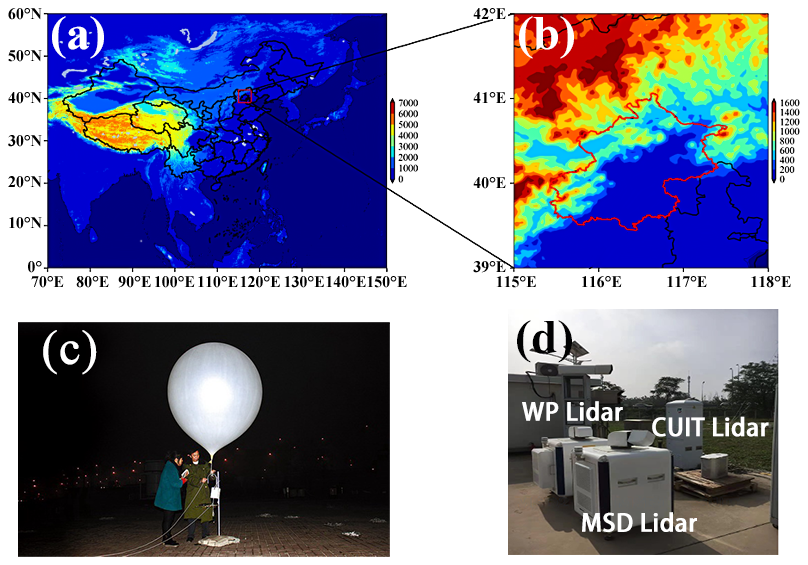
Figure 1 Location of the Nanjiao Observatory and instruments deployed during the campaign.

As shown in Fig. 1, Three coherent DWLs – MSD (Minshida Technology Co.), CUIT (homemade), and WP (WindPrint S4000) – were deployed alongside daily radiosonde launches. Both the MSD Lidar and CUIT Lidar employ single-frequency pulsed fiber lasers with a wavelength of 1550 nm. Aerosol molecules and large particles present in the air serve as tracers of the wind field. Coherent DWL retrieves the atmospheric wind field by measuring the backscatter of aerosols moving with the wind field (Weickmann et al., 2009).

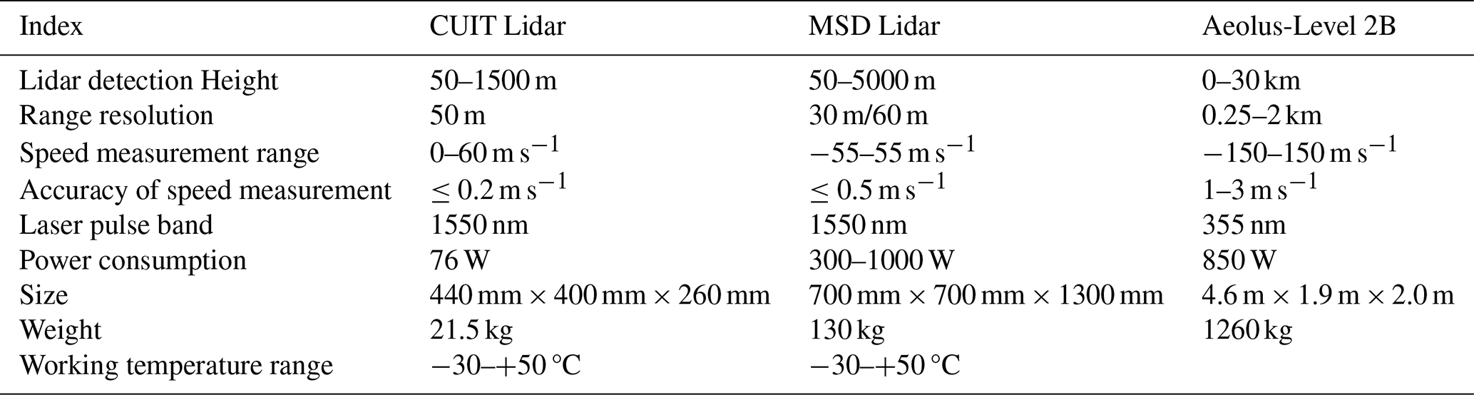
This study necessitates retrieving Aeolus satellite data from the European Space Agency (ESA) website (https://earth.esa.int/eogateway/catalog/aeolus-scientific-l2b-rayleigh-mie-wind-product, last access: 21 September 2025) for comparative analysis. Aeolus is a wind-profiling satellite, launched by ESA in 2018. It operates in a 320 km Sun-synchronous orbit, following a flight path approximately aligned with Earth's day-night terminator, completing an orbit every 90 min (Belova et al., 2021). The satellite is equipped with a 1.5 m diameter telescope, a scattering receiver to collect reflected signals, and a Doppler wind ultraviolet Lidar system named “Aladin”, which operates with an output power comparable to a small nuclear reactor and can penetrate the atmosphere up to 30 km altitude. Its working principle involves a processing system with a 1.5 m diameter aperture emitting pulsed ultraviolet laser beams (wavelength 355 nm) at a rate of 50 observations per second, with each beam generating billions of photons directed at the atmosphere. However, only a few hundred are scattered back to the satellite due to interactions with atmospheric molecules. The Doppler effect determines the time delay between emitted pulses and backscattered signals. The Doppler effect determines the time delay between emitted pulses and backscattered signals, and the wind field is observed by calculating the wind direction, speed, and displacement. The mean wind speed measurements are obtained by averaging the values obtained in vertical and horizontal directions. Vertical sampling is conducted within 24 altitude bins, ranging from 0.25 to 2 km.

A comparison of the technical specifications of Aeolus and other Lidars is presented in Table 1. The three Lidars use range gates to select specific distance ranges, measuring the velocity of aerosol particles within these ranges, and obtaining wind speeds at different altitudes. The Aeolus Level 2B (L2B) product is the Aeolus satellite's primary wind field product. It provides horizontal line-of-sight (HLOS) wind speed observations that have been atmospheric corrected and geo-located, extracting the necessary L2B data variables, such as the latitude, longitude, and wind speed information within the observation time range. The L2B product also provides scene classification based on the backscatter ratios corresponding to winds from “cloudy” or “clear” atmospheric regions, generating observation types such as “Rayleigh-clear”, “Rayleigh-cloudy”, and “Mie-cloudy” (Borne et al., 2024; Martin et al., 2021).

The satellite-Lidar comparison in the article refers to the method proposed by Guo et al. (2021). The Aeolus Level 2B wind products represent averages over specific vertical bins (each bin spanning 0.25–2 km in height), while ground-based instruments achieve resolutions of 30 m/50 m/60 m. Preprocessing Steps as follows:

• Step 1: Partition the high-resolution ground-based lidar data according to Aeolus's vertical bin boundaries.

• Step 2: Average the ground-based data within each bin to generate vertical-layer-averaged wind fields corresponding to Aeolus.

• Step 3: Project the averaged wind fields onto Aeolus's line-of-sight (HLOS) direction for comparison.

Table 1 Instruments Technical Index.

Figure 2 The flow of Lidar and radiosonde dataset height matching.

2.2 Data processing

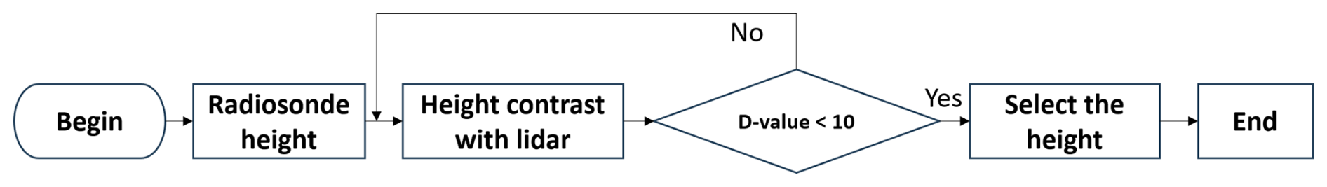
The collected data often have outliers in the DWL measurement process. Data use quality control can obtain accurate information about the changes in the atmospheric wind profile, which is helpful to understand and predict the atmospheric motion pattern. As shown in Fig. 2, the wind speed and direction data from the radiosonde, CUIT Lidar, MSD Lidar, and WP Lidar are height-matched through the implementation of the sliding window method, producing a comprehensive dataset that is arranged sequentially based on time, altitude, wind direction, and wind speed. This dataset serves as the foundation for subsequent analyses. The sliding window method, widely used in signal processing and time series analysis, was applied to align datasets. This method involves strategically restricting the maximum number of data points that each window can accommodate, as previously outlined in the extant literature (Wang et al., 2023; Zhao et al., 2024a). The specific matching process, using the radiosonde height and CUIT Lidar height as an example, employs a sliding window of size 3, moving two positions to the right each time. In each window, a value is selected and compared with the CUIT Lidar height, with the closest value being selected as the matched radiosonde height.

When measuring wind speed, sudden peaks often result in anomalous values. The isolation forest (IF) model is used to filter the data to identify and remove these anomalies. IF (Liu et al., 2008) is an unsupervised anomaly detection algorithm that effectively identifies anomalies in a dataset by isolating outliers (Hernandez-Mejia et al., 2024). The algorithm recursively partition data points into subsets using randomly selected features and thresholds (Borne et al., 2024). Anomalies require fewer partitions to isolate them from other data (Liu and Aldrich, 2024). Anomalous values have the characteristic of being few and significantly different from normal values. The IF can separate and remove anomalies without modeling the normal data, and identify anomalous data accurately. In constructing the binary tree structure, fewer partitions are required to isolate anomalous data, which is closer to the root, and normal data is further from the root. This feature allows for effective anomaly detection. The CUIT data is complete without any omission. The one with the most missing data is CUIT Lidar, where 426 out of a total of 2885 data points are missing, the missing rate reaches 14.8 %. The second one is WP Lidar, there are 46 missing data points, accounting for 1.6 % of the total 2885 points. The following algorithm will be used to optimize missing and anomalous data.

2.2.1 Isolation tree

Let T be a node of the isolation tree (iTree). T has two possibilities: it is either a leaf node with no children or an internal node with a test and exactly two children. (T_lT_r). The test is composed of an attribute q and split value p, where p>q, which divides the data points into T_l and T_r.

The sample data $X=\mathit{\{}{x}_{\mathrm{1}}{x}_{\mathrm{2}},\mathrm{\dots },x_n\mathit{\}}$ where n represents the number of instances in the distribution. The iTree is recursively constructed by splitting based on the attribute q and split value p. The splitting process terminates when the tree reaches the height limit (|X|=1), or when all instances in X have the same value.

2.2.2 Anomaly detection

For anomaly detection, the method primarily ranks data points based on path length or anomaly score, with the points at the top being considered anomalous.

Path length: The path length h(x) of point x is calculated as the distance from the root node of the iTree to the leaf node for point x.

Anomaly score:

After getting the path length h(x), the outlier scour of x is as follows:

$$\begin{array}{}\text{(1)}& {\displaystyle }S\left(xu\right)={\mathrm{2}}^{-\frac{E\left(h\right)}{C\left(u\right)}}\text{(2)}& {\displaystyle }C\left(u\right)=\mathrm{2}H\left(u-\mathrm{1}\right)-{\displaystyle \frac{\mathrm{2}(u-\mathrm{1})}{u}}\end{array}$$

where the u is the number of samples, and C(u) is the average path length of all data in the training set. H(i) is harmonic number, ln (i)+0.5772156649. E(h) is the average path length of x across n iTrees.

1. When $E\left(h\right)\to C\left(u\right),S\to \mathrm{0.5}$;

2. when $E\left(h\right)\to \mathrm{0},S\to \mathrm{1}$;

3. when $E\left(h\right)\to u-\mathrm{1},S\to \mathrm{0}$;

Evaluate and remove outliers based on the anomaly score.

1. If S(xu) approaches 0.5, the outlier becomes less apparent.

2. If S(xu) approaches 0, the score is normal value.

3. If S(xu) approaches 1, the value is anomalous.

2.3 Random forest for lidar data

To address the missing values after Lidar detection and after outlier removal, this study uses RF to correct the Lidar data. In the correction of Lidar data, the wind speed and direction at each altitude layer are treated as samples. Considering the uncertainties and errors in the original data, the RF is used for correction. By integrating multiple decision trees, RF can effectively handle and analyze high-dimensional complex data, accurately predicting wind speed and direction, thereby improving wind field data's supplementation and prediction capabilities. It is important to note that the performance of the RF model largely depends on the quality of the training data and the selection of features. Additionally, attention should be given to the issue of overfitting, and the model should be optimized and adjusted based on actual conditions. The RF model in this research is built as follows: Step 1: Extract a sub-sample matrix from the training matrix as the training samples.

Step 2: Each sample has M features. Specify a constant m where m≪M and randomly select a subset of m features from the M features. Finally, select the optimal feature subset for regression.

Step 3: Allow the tree to continuously split until a certain height is reached.

Step 4: Repeat the previous three steps until the regression tree is fully constructed and trained. The final output model is the “ensemble predictor” f(x). The ensemble predictor f(x). is composed of the “base learners” $h_{\mathrm{1}}\left(x\right),\mathrm{\dots },h_J\left(x\right)$ (Cutler et al., 2012):

$$\begin{array}{}\text{(3)}& f\left(x\right)={\displaystyle \frac{\mathrm{1}}{J}}{\sum }_{j=\mathrm{1}}^J{h}_J\left(x\right)\end{array}$$

Figure 3 The total flow of data processing.

2.4 Lidar data correction

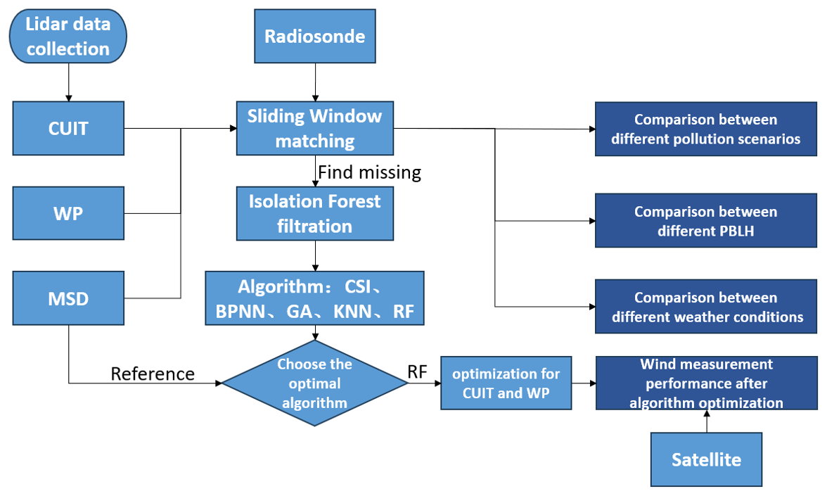
The overall data processing workflow is shown in Fig. 3. After matching the wind direction and wind speed data from the three Lidars with radiosonde data using the sliding window method, the data is compared under different pollution conditions, PBLH, and weather conditions to identify the optimal performing Lidar and the Lidar that requires improvement. For missing values caused by the instrument itself or following anomaly cleaning, cubic spline interpolation (CSI), back propagation neural network (BPNN), Genetic Algorithm (GA), k-nearest neighbor (KNN), and RF were used to fill the missing values. By comparing the correlation of each algorithm, the most suitable algorithm is identified for the final Lidar data optimization, the Aeolus satellite is used to verify the reliability of the algorithm further.

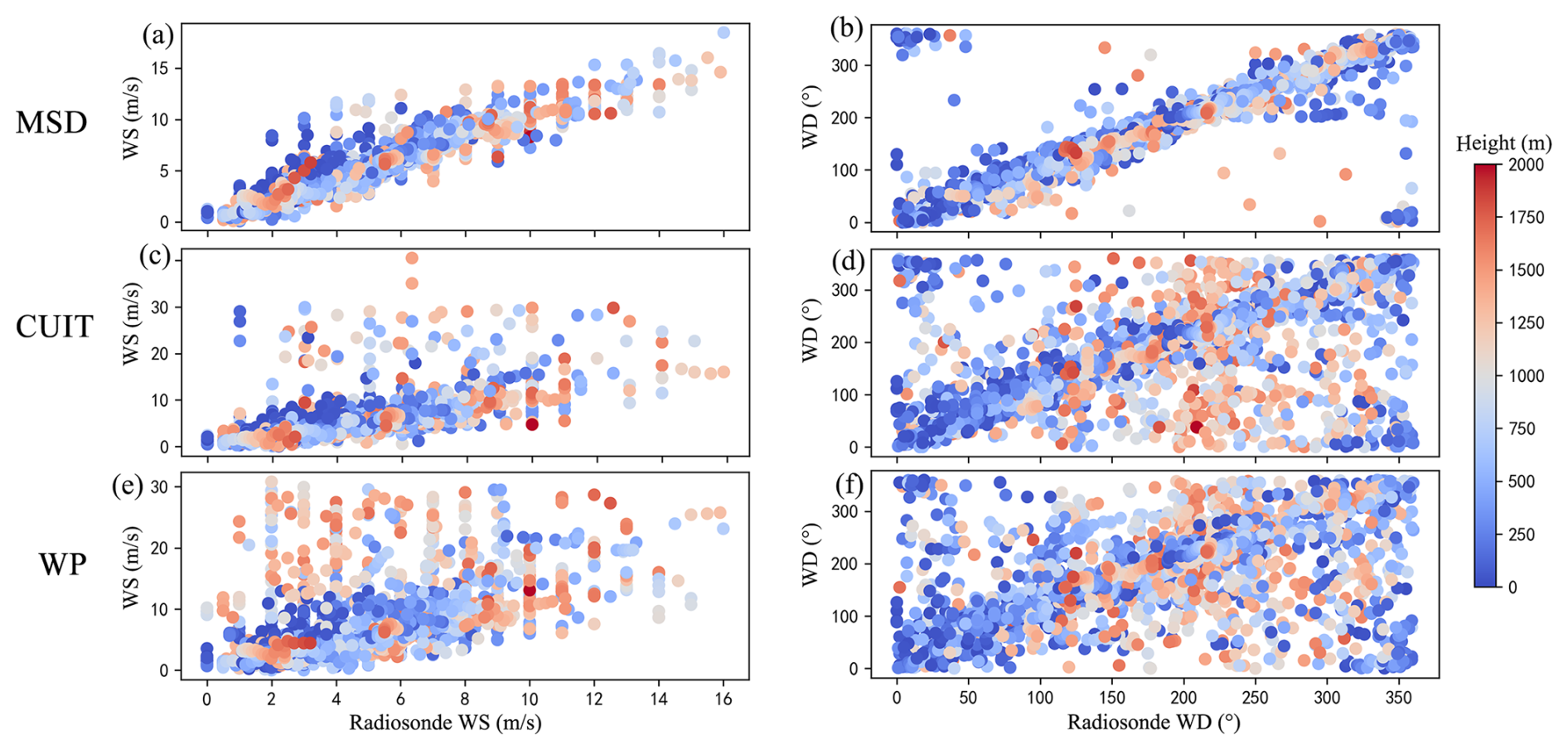
Figure 4 (a) WS and (b) WD of radiosonde data and MSD Lidar at different heights; (c) WS and (d) WD of WP Lidar; Comparison of (e) WS and (f) WD of CUIT Lidar; color bar represents height.

3 Results and discussion

3.1 Performance comparison of Doppler wind lidars

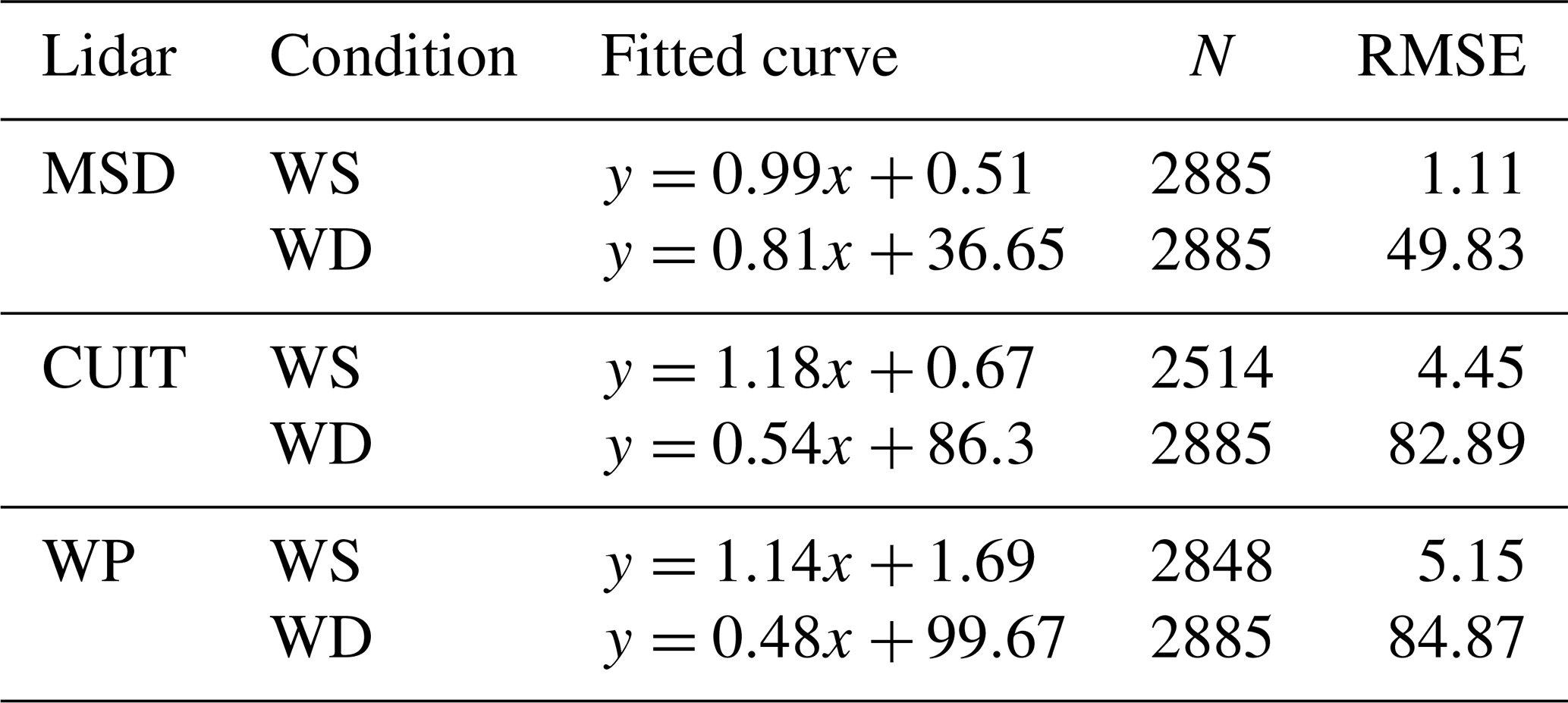
Figure 4 compares wind speed and direction data from MSD Lidar, CUIT Lidar, and WP Lidar with the radiosonde data at different heights. The dispersion of the scatter points represents the correlation between the Lidars and the radiosonde data. The WD was defined as the range from 350 to 10°, and all winds within this range were classified as northerly, which were not considered anomalies in the study. As shown in Fig. 4, MSD Lidar, CUIT Lidar, and WP Lidar exhibited good consistency with the radiosonde data in the low-altitude region below 600 m. However, as the altitude increased, the dispersion of wind speed and direction from the three Lidars gradually increased, especially above 1500 m. Regression parameters of three Lidars and radiosonde data are summarized in Table 2. MSD Lidar had a wind speed and direction slope of 0.99 and 0.81, respectively, with RMSE values of 1.11 m s⁻¹ and 49.83°, which were closest to the radiosonde data. CUIT Lidar showed significant anomalies below 750 and above 1500 m, with wind speed overestimated, and wind direction RMSE reaching 82.89°. The performance of WP Lidar exhibited an overestimation of wind speed across all heights. Notably, the magnitude of errors was particularly pronounced in high-altitude regions, as evidenced by wind direction RMSE reaching 84.87°. Overall, the observation data in the low-altitude region (blue) were more stable. In contrast, the high-altitude region (red) decreased observation accuracy for all three Lidars due to altitude effects. This reveals an exponential decay trend in Lidar measurement accuracy with increasing altitude, consistent with the attenuation characteristics of Lidar backscatter signals. These results provide critical insights for high-precision wind field monitoring: The MSD Lidar is the preferred choice for boundary layer observations (<1.5 km). At the same time, real-time radiosonde data correction is advised for elevated altitude applications.

Table 2 Regression parameters of three Lidars and radiosonde.

3.2 Comparative analysis of performance under different air quality conditions

To investigate the performance of three DWLs in measuring wind speed and direction under different aerosol mass concentrations, the experiment integrated PM_2.5 concentration data from collaborative observations with wind profile analysis. The PM_2.5 concentrations are relatively low at the site, so the concentration range was divided into three pollution levels: L1 (PM_2.5=0–15 µg m⁻³), L2 (PM_2.5=15–35 µg m⁻³), and L3 (PM_2.5=35–50 µg m⁻³) (Wu et al., 2016). Figure 5a–c present Scatter plots of wind speed regression relationships for the MSD, CUIT, and WP Lidars across these pollution tiers, with linear regression lines for L1 (red), L2 (green), and L3 (yellow). The results show the correlation of the three Lidars in different pollution levels. It is evident that aerosol concentrations significantly affect the performance of Lidar in wind speed detection. The regression parameters of the three Lidars and radiosonde under different pollution conditions are summarized in Table 3. During L3 pollution episodes, MSD Lidar achieves the highest correlation with the radiosonde (R²=0.82), demonstrating strong stability and reliability. In contrast, CUIT Lidar and WP Lidar show much lower correlations under L3 conditions ($R_{\mathrm{CUIT}}^{\mathrm{2}}=\mathrm{0.24},R_{\mathrm{WP}}^{\mathrm{2}}=\mathrm{0.04}$), indicating that their detection performance is significantly affected by air quality. Under L1 conditions, the correlations for CUIT Lidar and WP Lidar are R²=0.35 and R²=0.32, with RMSE values of 1.43 and 1.36 m s⁻¹, respectively. Under L2 conditions, the correlations decrease to R²=0.3 and R²=0.17, with RMSE values of 1.45 and 1.39 m s⁻¹, respectively. Aerosol mass concentration has a negative impact on the detection performance of DWL, particularly for CUIT and WP Lidars, which exhibit significant performance degradation under higher pollution levels. No data were collected under heavy pollution conditions (>50 µg m⁻³ PM_2.5) during the experiment, which may be attributed to a decline in performance above 50 µg m⁻³.

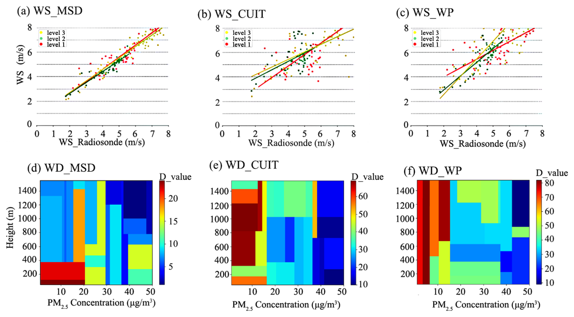
Figure 5 Comparison of radiosonde data with CUIT, MSD, WP (a–c) WS, and (d–f) WD at different heights and PM_2.5 concentrations.

The wind direction difference can be used to evaluate the impact of different aerosol mass concentrations on the performance of DWL. Due to the periodic nature of wind direction data, the absolute value of the wind direction difference was calculated, and differences exceeding 180° were excluded from the analysis. Figure 5d–f illustrates the distribution of wind direction differences as a function of PM_2.5 concentration and height. The x-axis represents aerosol mass concentration, the y-axis represents height, and the colorbar represents the wind direction difference. The MSD Lidar exhibits high detection accuracy, maintaining wind direction deviations within 20°. Under the L1 air quality, maximum deviations (D>20°) occur below 400 m altitude, while within the 400–1400 m range, deviations remain below 10°. For L2 conditions within this height band, deviations increase to 17.5°. The wind direction difference of MSD Lidar remains below 7.5° at altitudes above 1 km, indicating high accuracy in high-altitude detection, though with certain limitations under low aerosol concentration conditions. The CUIT Lidar demonstrates a heightened wind direction difference of 40–65° when PM_2.5 concentrations fall below 17 µg m⁻³. When PM_2.5 concentrations increase to 17–37 µg m⁻³, the deviation reduces to 30–40°. As PM_2.5 concentrations increase (>40 µg m⁻³), the difference significantly decreases to 10–25°, indicating improved accuracy under higher pollution conditions. The WP Lidar demonstrates the poorest performance (<15 µg m⁻³ PM_2.5), with deviations reaching 50–80°. However, when PM_2.5 concentrations exceed 40 µg m⁻³ and altitudes exceed 800 m, deviations significantly reduce to about 10°. WP's performance above 800 m improves with deviations within 20° under L3 conditions. The observed accuracy enhancement with increasing aerosol concentrations (>800 m altitude) likely stems from amplified laser backscattering signals caused by atmospheric particulates. This phenomenon particularly improves wind field retrieval accuracy in elevated regions. Operational deployment of DWL systems in polluted environments requires careful consideration of both instrument specifications and ambient aerosol characteristics. Overall, the observed performance improvement at L3 (35–50 µg m⁻³) concentrations reflects that the Lidar requires a certain amount of aerosol backscattering.

Table 3 Regression parameters of three Lidars and radiosonde under different pollution conditions.

3.3 PBLH's impact on Doppler wind lidars

Aerosol concentrations exhibit a pronounced inverse correlation with PBLH variations. During daytime, convective updrafts enhance PBLH development, which promotes vertical diffusion of aerosols and reduces their near-surface concentrations (Paul and Das, 2022; Su et al., 2018). This section quantifies explicitly the sensitivity of Lidar wind field retrievals to PBLH stratification. Performance evaluations of three Lidar systems (MSD, CUIT, and WP Lidar) against radiosonde measurements were conducted across PBLH and CBH used by the ERA5 datasets. The time resolution of the PBLH and CBH of the ERA5 reanalysis data is one hour. The three Lidars matched the time and altitude through the sliding window method. Because of the linear relationship, the Pearson correlation coefficient (PCC) was chosen to represent the correlation with the radiosonde. As shown in Fig. 6, the MSD Lidar exhibited a correlation higher than 0.85 with radiosonde wind speed across all height intervals, demonstrating strong accuracy and insensitivity to PBLH variations. However, its wind direction correlation notably decreased to 0.53 within the 1500–1750 m PBLH range, likely attributable to enhanced aerosol-layer complexity at elevated mixing heights and the small samples in this range (N=41). Although the sample size within this PBLH is relatively less, wind speed was unaffected; only the poor performance in wind direction was particularly prominent. This may be due to complex turbulent structures and aerosol distributions leading to wind direction instability in high PBLH regions (Lothon et al., 2009; Su et al., 2020; Yamartino, 1984). Outside this interval, wind direction correlations remained robust (>0.70), indicating superior overall performance. The CUIT Lidar showed a wind speed correlation generally above 0.7, its performance was optimal in the 500–750 m PBLH range (ρ_WS=0.92, ρ_WD=0.75), but its wind speed decreased to 0.6 at a PBLH of 1000–1250 m. The wind direction correlation dropped below 0.4 when PBLH exceeded 1500 m, reflecting limitations in high-altitude detection. The WP Lidar showed significant deficiencies in wind speed detection, with correlations below 0.72 across all height intervals, and its performance declined notably with increasing PBLH.

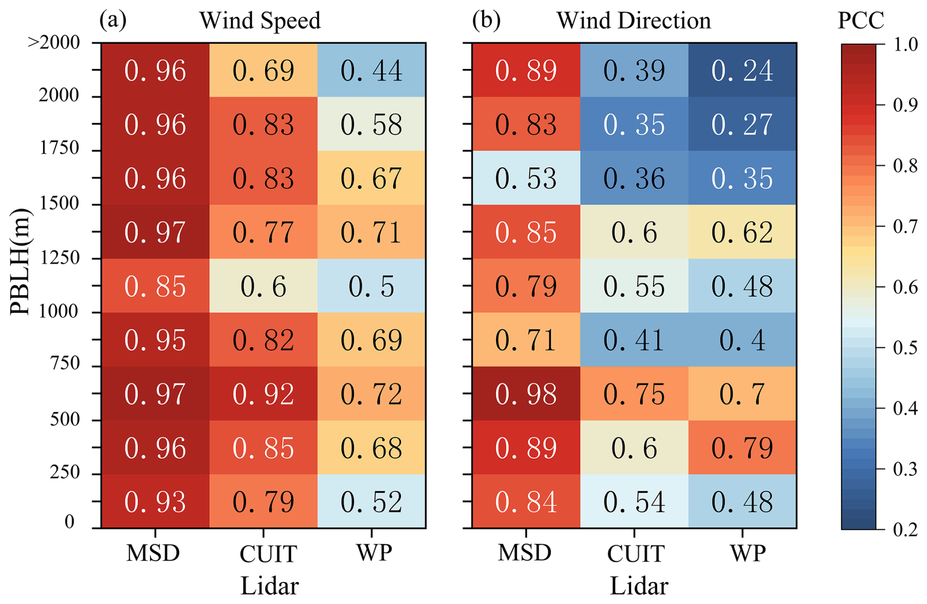
Figure 6 Comparison of (a) WS and (b) WD between radiosonde data and CUIT Lidar, MSD Lidar, and WP Lidar at different PBLH; Color bar represents Pearson correlation coefficient.

This may be attributed to the principle of DWL, which posits that backscattering signals from aerosols play a critical role in wind speed measurement, particularly within the boundary layer and lower troposphere (He et al., 2022b; Li and Yu, 2018; Tan et al., 2019). The performance of Lidar is influenced by the distribution of particles, which is affected by different PBLH levels. At lower altitudes (<750 m), all three Lidars demonstrated optimal performance, likely due to stable wind speed and direction, and minimal turbulence within this range, resulting in superior Lidar measurement accuracy. Conversely, the wind direction measurement performance declined substantially at higher altitudes (>1500 m).

To further investigate the influence of PBLH on Lidar performance, the vertical relationship between CBH and PBLH (both derived from ERA5 data) was introduced to analyze atmospheric impacts on Lidar measurements. As illustrated in Fig. 6, two distinct PBLH ranges, 1000–1250 and 500–750 m, were selected to examine contrasting Lidar performance (superior vs. inferior). The WS and WD performance of three Lidars under varying CBH and PBLH conditions is summarized in Table 4.

When PBLH was elevated (1000–1250 m) with low clouds (CBH <1 km), the PCCs for MSD are 0.85 (WS) and 0.93 (WD). Under shallow PBLH (500–750 m) with higher clouds (CBH >750 m), MSD exhibited significantly improved PCCs of 0.97 (WS) and 0.98 (WD), maintaining its superior performance. Notably, MSD and CUIT Lidars dominated in WS correlation (PCCs: 0.85 and 0.59, respectively) under high PBLH conditions (1000–1250 m, CBH <1 km), which is similar to Fig. 6. In this case, the coupling ratio between cloud and PBLH is as high as 90 % (Su et al., 2022), the atmosphere is usually accompanied by higher relative humidity (Liu, 2019), the turbulent mixing effect in the boundary layer is enhanced, and the vertical distribution of aerosols becomes complicated, all of which exacerbated Lidar signal interference. Conversely, PBLH was elevated (500–750 m) with high clouds (CBH >750 m), WD correlations dominated across all three Lidars (PCCs: 0.98, 0.65, and 0.59). The decoupling between clouds and the boundary layer fostered a stable vertical structure, confining aerosols and turbulence predominantly below the PBLH. This stratification minimized cloud-induced signal attenuation, enabling clearer detection of vertical wind profiles.

Table 4 The WS and WD performance of three Lidars under varying CBH and PBLH conditions.

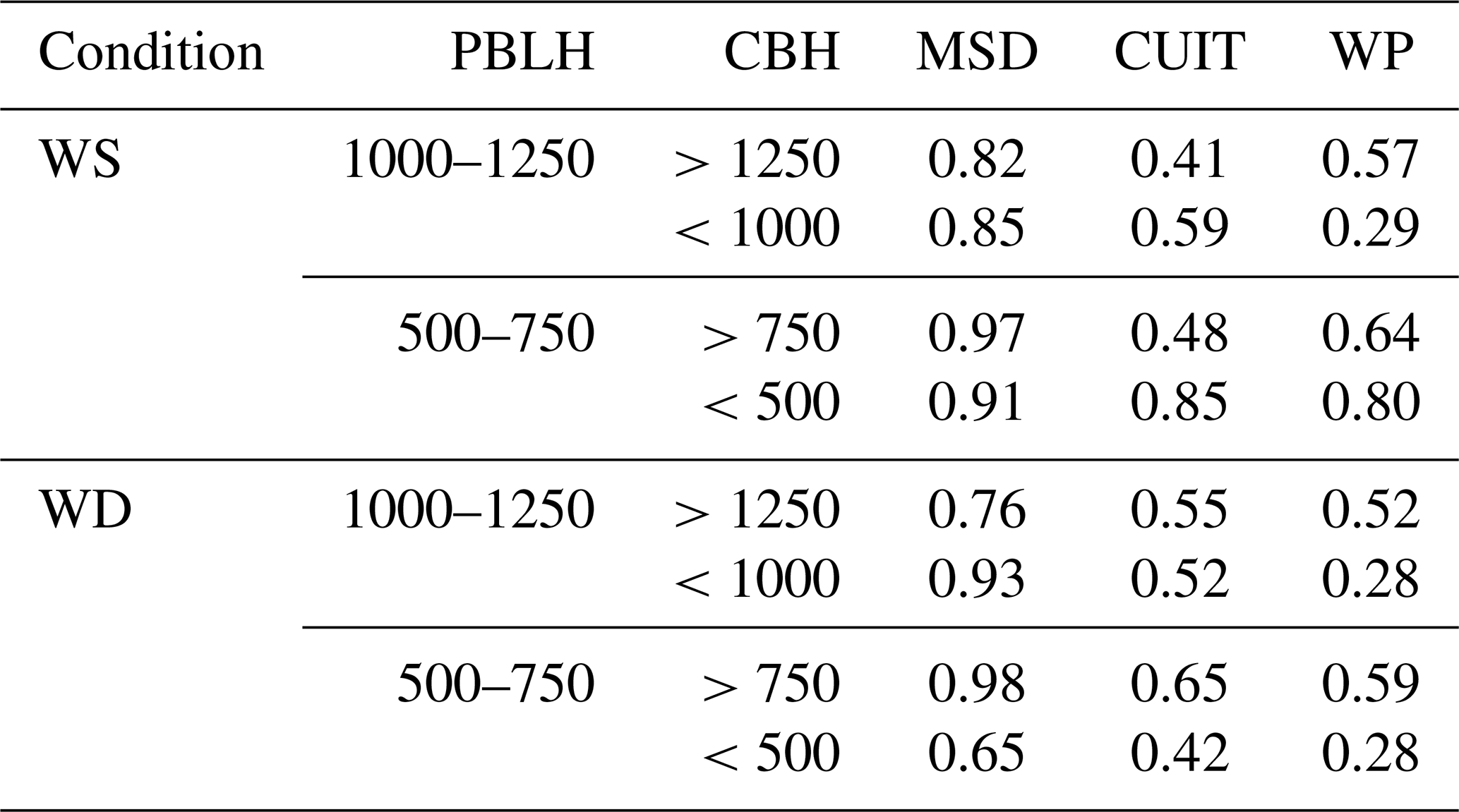
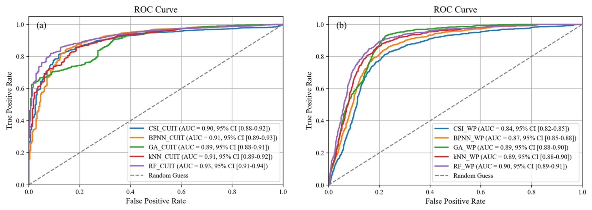
Figure 7 The ROC Curves between three Lidars and radiosonde after interpolation using five algorithms.

3.4 Analysis of correction results of random forest algorithm

The IF filtering identified additional data gaps in both CUIT and WP Lidar datasets. To maintain temporal continuity, anomalous values were replaced with NaN rather than row deletion. Five interpolation algorithms – CSI, BPNN, GA, k-NN, and RF – were implemented to enhance data reliability. Fig. 7 shows the comparison of the Receiver Operating Characteristic (ROC) curves of five optimization algorithms. The Area Under the Curve (AUC) metrics, accompanied by 95 % confidence intervals (CI) derived from bootstrap resampling (n=1000). Random forest (RF_CUIT and RF_WP) demonstrated superior performance with the AUC of 0.93 (95 % CI [0.91–0.94]) and 0.90 (95 % CI [0.89–0.91]), underscoring its robustness in modeling non-linear relationships and high-dimensional atmospheric data. This aligns with its inherent capability to handle complex interactions within lidar-derived wind profiles. CSI's inherent locality is characterized by using cubic functions to connect adjacent points (Komsta, 2010). This approach entails global fitting, thereby rendering any alteration in a single data point capable of affecting the entire curve. This heightened sensitivity can make the spline curve more uneven and challenging to manipulate, particularly for functions comprising linear segments or sudden alterations (Maglevanny and Smolar, 2016). Wind speed may exhibit nonlinear or abrupt variations over time and space under higher altitudes or complex airflow conditions. Cubic spline interpolation struggles to capture such non-smooth dynamic changes effectively, leading to increased interpolation errors. For BPNN, the sufficiency and efficiency of the training set are critical factors influencing generalization (Singh et al., 2023). With limited wind speed data, there is a risk of overfitting or underfitting, which may lead to unstable performance. Due to the inherent randomness of genetic operations, the GA does not always produce optimal solutions, although it can find suboptimal solutions within a reasonable time (Jurasovic and Kusek, 2010). While GA excels in global optimization, its iterative nature might hinder real-time processing efficiency, a critical factor for operational Lidar systems. The k-NN algorithm is sensitive to local data structures, performing poorly in regions with sparse observations or high volatility (Gupta et al., 2020). The RF algorithm can handle high-dimensional datasets and capture complex nonlinear relationships effectively (Grimm et al., 2008; Horemans et al., 2020). RF minimizes the risk of overfitting, resulting in more reliable predictions by aggregating multiple decision trees (Grimm et al., 2008; Horemans et al., 2020; Li et al., 2023). Regarding interpolation, RF can effectively handle missing values, ensuring that the model remains robust and accurate (Xu et al., 2024). The iterative hyperparameter tuning process optimized RF's performance, confirming its suitability for DWL data correction under complex atmospheric conditions.

In summary, all algorithms significantly outperformed the random guess baseline (AUC =0.5), and the confidence intervals across all methods are narrow (<0.04 AUC range), confirming their utility and reliability in wind data refinement. recommended. RF is recommended for Lidar applications, prioritizing accuracy due to its high AUC and stable CI. These findings highlight the importance of algorithm selection tailored to specific operational requirements in atmospheric remote sensing.

To achieve optimal interpolation results, a parameter grid was defined with “mtry” and “ntree”. “mtry” represents the number of features considered at each split in the RF, with mtry $\in [\mathrm{1},\mathrm{10}]$, and “ntree” represents the number of trees, with ntree $\in [\mathrm{100},\mathrm{500}]$. The parameter grid was iteratively traversed in the training function to identify the optimal parameter configuration, with a fixed random seed ensuring computational reproducibility.

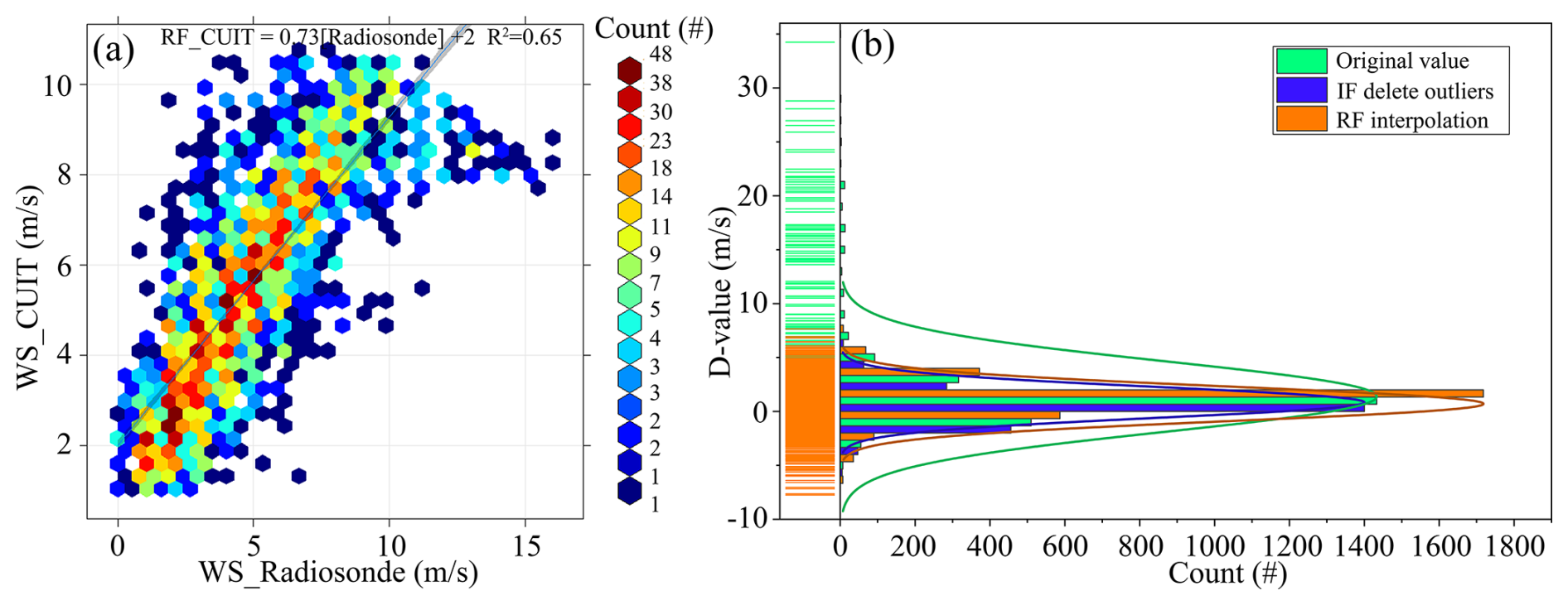
Figure 8 (a) WS scatter plot of CUIT Lidar and radiosonde after processing; (b) Comparison distribution map of the difference between CUIT and radiosonde after IF and RF processing.

Figure 8a shows the scatter plot of wind speed data after removing anomalies using the IF and interpolating missing values with RF. Initial CUIT Lidar wind speed data exhibited poor agreement with radiosonde measurements (R²=0.42). Following anomaly removal via the IF and RF-based interpolation, correlation improved significantly (R²=0.65). The RF interpolation led to a more complete data distribution, with missing values being compensated for.

Figure 8b shows the distribution of differences between CUIT Lidar and radiosonde data after algorithmic processing. The original CUIT data (green) exhibited a wide distribution with a maximum difference of 34 m s⁻¹. The peak of the difference was not concentrated near 0 m s⁻¹. After filtering the data with IF (blue), anomalies were removed, and the differences became more concentrated within −3–3 m s⁻¹. The IF effectively identifies and outliers, allowing the remaining data to better align with the radiosonde trend. After optimizing and supplementing the data using the RF algorithm (orange), the wind speed data became closer to the radiosonde data, with the peak difference aligning at 0 m s⁻¹. The range of the difference distribution further narrowed, demonstrating a high consistency between the interpolated CUIT Lidar data and the radiosonde data. The orange histogram exhibited significantly superior symmetry and concentration compared to the blue histogram, RF not only repaired missing values but also preserved the global characteristics and trends of the data. In summary, the enhanced peak concentration of the difference distribution validates the applicability and reliability of the RF model in correcting nonlinear data. These improvements are particularly pronounced in low-altitude regimes (<1 km), where boundary layer turbulence amplifies measurement uncertainties.

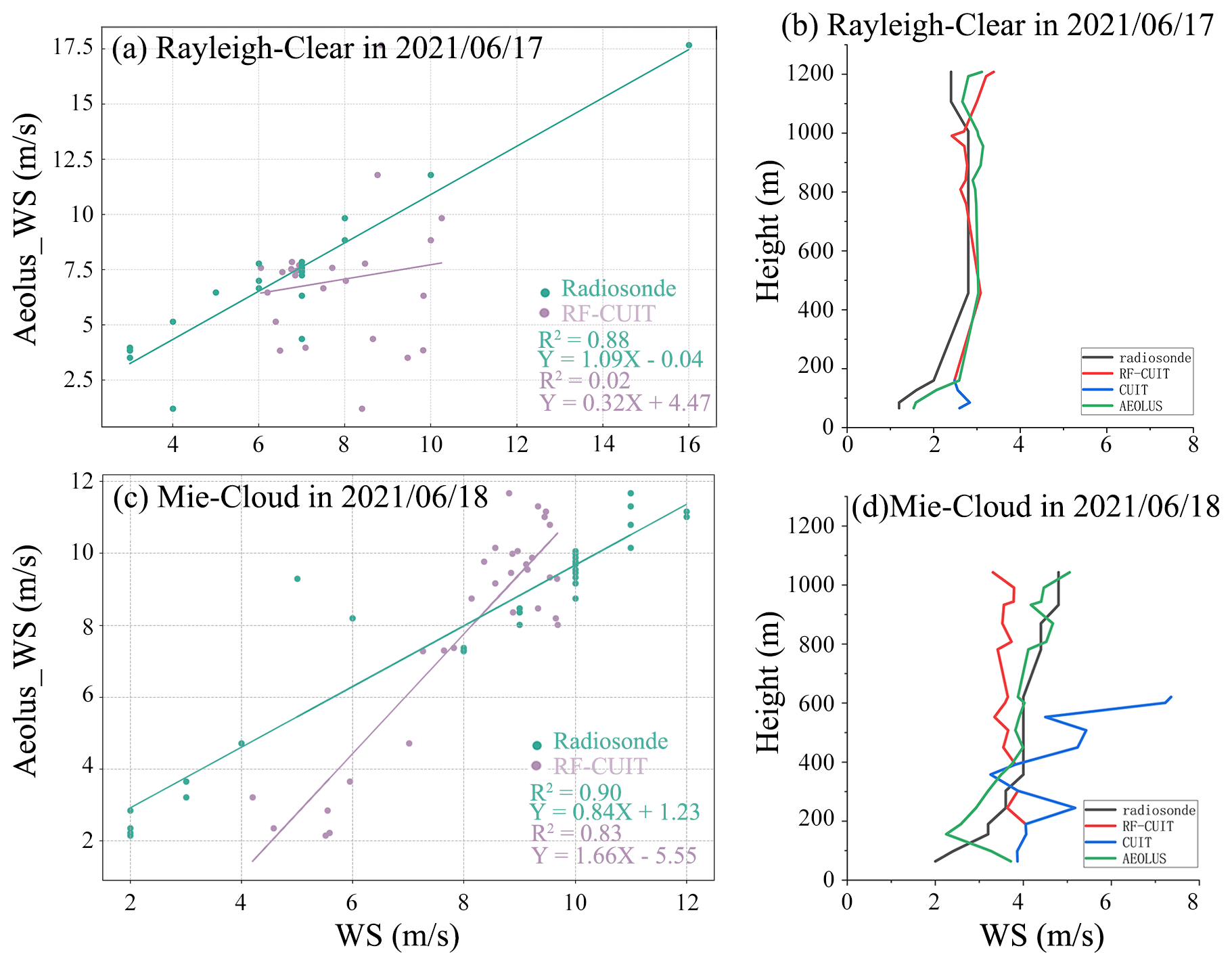
Figure 9 The relationship between interpolated CUIT Lidar, radiosonde, and Aeolus satellite data in the (a) Rayleigh and (c) Mie channels; and (b, d) a profile plot from a single radiosonde observation.

3.5 Aeolus verification

As shown in Fig. 9, comparative analysis of Aeolus satellite products revealed enhanced wind speed retrieval precision under cloudy conditions (Mie-channel R²=0.90) compared to clear-sky retrievals (Rayleigh-channel R²=0.88. This performance differential stems from amplified backscatter signals through cloud-aerosol interactions, underscoring the critical role of atmospheric particulates as natural scattering tracers for optimizing spaceborne wind profiling.

The Aeolus satellite exhibits high consistency with radiosonde data in both channels, indicating the feasibility of using Aeolus for Lidar data validation. A case for a radiosonde observation on 17 June 2021, as shown in Fig. 9a and b, indicates that CUIT Lidar data had a high proportion of missing values, with a missing rate of up to 80 %. However, in this case, the application of RF for interpolation led to a substantial enhancement in the congruence between CUIT Lidar and radiosonde data, particularly within the 0.5–1 km altitude range. During the radiosonde observation on 18 June in Fig. 9c and d, the IF successfully identified and removed anomalies in the 200–600 m range. Following RF interpolation, the correlation between CUIT Lidar and Aeolus satellite data exhibited a substantial enhancement, with R² reaching 0.83. This outcome signifies that this method can effectively enhance data quality and accuracy, even in anomalies. But that reflects agreement on the scale resolvable by Aeolus, not necessarily the full resolution of the Lidar. Integrating Aeolus validation and RF-based correction establishes a robust framework for enhancing Lidar data reliability. These findings validate the ability of machine learning for complex atmospheric data reconstruction.

4 Conclusions

This study was conducted at the Nanjiao Observatory in Beijing from 9 June to 31 August 2021, using three ground-based DWLs (MSD, CUIT, and WP) and simultaneous radiosonde data to evaluate the performance of the Lidars under different conditions.

The results show that all Lidars demonstrate strong concordance with radiosonde wind speed measurements at the low altitude of 600 m. As altitude increases, the deviations in wind speed and direction from the three Lidars gradually increase. The RMSE of wind speed for MSD Lidar is 1.11 m s⁻¹, 4.45 m s⁻¹ for CUIT Lidar and 5.15 m s⁻¹ for WP Lidar. In terms of wind direction, MSD Lidar exhibited the most accurate performance, with an RMSE of 49.83°, CUIT Lidar with an RMSE of 82.88°, and WP Lidar exhibited the most significant deviation with an RMSE of 84.87°. Among the three Lidars, MSD Lidar exhibited the highest accuracy in wind speed and wind direction measurements, closest to radiosonde measurements.

The correlation and accuracy of wind speed measurements from MSD Lidar with radiosonde data were optimal under varying pollution conditions, as evidenced by R² values of 0.76, 0.65, and 0.82 for L1, L2, and L3 pollution conditions, and RMSE values of 0.79, 0.47, and 0.66 m s⁻¹, respectively. Additionally, under light pollution conditions with aerosol mass concentrations of 0–15 µg m⁻³, MSD Lidar exhibited the highest correlation with radiosonde wind speed, demonstrating its intense sensitivity to aerosol mass concentrations. When the aerosol concentration in the lower atmosphere increases to a certain level (40–50 µg m⁻³), Lidar can facilitate better signal reception by scattering improvement. Consequently, it is imperative to consider the impact of varying aerosol mass concentrations when detecting low-altitude wind fields to ensure the optimal performance of Lidar instruments.

The PBLH significantly influences Lidar performance, with the most effect observed at PBLH of 1000–1250 m, and the optimal performance at lower altitudes (500–750 m). MSD and CUIT Lidars dominated in WS correlation (PCCs: 0.85 and 0.59, respectively) under high PBLH conditions (1000–1250 m, CBH <1 km). The turbulent mixing effect in the boundary layer is enhanced, and the vertical distribution of aerosols becomes complicated, which exacerbates Lidar signal interference. Conversely, PBLH was elevated (500–750 m) with high clouds (CBH >750 m), WD correlations dominated across all three Lidars (PCCs: 0.98, 0.65, and 0.59). The decoupling between clouds and the boundary layer fostered a stable vertical structure. This stratification minimized the cloud-induced signal attenuation.

Five algorithms interpolation (CSI, BPNN, GA, k-NN, and RF) was applied to CUIT and WP Lidar, the RF demonstrated superior performance with the AUC of 0.93 (95 % CI [0.91–0.94]) and 0.90 (95 % CI [0.89–0.91]) in the ROC curves. And RF-based correction of CUIT enhanced R² from 0.42 to 0.65, bringing it into closer alignment with the radiosonde data. This outcome underscores the efficacy of the RF correction algorithm, its reliability, and its aptitude for managing high-dimensional and incomplete data.

The cloud cover has a significant impact on the DWL measurement by the comparative analysis with the Aeolus satellite product, the results revealed enhanced wind speed retrieval precision under cloudy conditions (Mie-channel R²=0.90) compared to clear-sky retrievals (Rayleigh-channel R²=0.88). In the case of severe anomalies, the correlation between CUIT Lidar and satellite data is significantly enhanced after RF interpolation, and R² reaches 0.83.

Overall, this study sheds light on the different factors affecting the DWLs of wind speed and wind direction, including different aerosol mass concentrations, PBLH and CBH conditions, Machine learning, and Satellites, and the combination of IF and RF algorithms can effectively improve the quality and accuracy of wind field data for the future research of low-altitude detection.