the Creative Commons Attribution 4.0 License.
the Creative Commons Attribution 4.0 License.
 | 25 Sep 2025
Synergy of millimeter-wave radar and radiometer measurements for retrieving frozen hydrometeors in deep convective systems
Hirohiko Masunaga
Satellite remote sensing of frozen hydrometeors in deep convective systems is essential for understanding precipitation systems and the formation of upper-level clouds. To reduce uncertainties in ice cloud microphysical properties inside convective clouds, a combined use of millimeter-wave sensors sensitive to frozen particles in deep convective clouds is a promising strategy. This study uses the CloudSat Cloud Profiling Radar (CPR) and the Global Precipitation Measurement (GPM) Microwave Imager (GMI) to retrieve the vertical profiles of ice water content (IWC), number concentration (Nt), and mass-weighted diameter (Dm). A new retrieval method is developed by a combination of a deep neural network (DNN) and an optimal estimation method (OEM). In the first step of the algorithm, an initial guess is estimated by DNN based on an a priori database, followed by the next step where OEM seeks a more optimal frozen hydrometer profile.
The retrieval performance is evaluated against selected match-up observations of CloudSat and GPM. The combined use of CPR and GMI observations reduces retrieval errors compared to the CPR-only observations. The retrieved frozen hydrometer profiles excellently reproduce CPR reflectivity and GMI brightness temperatures (Tb) when computed by forward simulations. The Dual-frequency Precipitation Radar (DPR) reflectivity is also reasonably reproduced, indicating some ability to retrieve large snow and graupel particles detectable by the low-frequency radars. A significant spread in simulated Tb is found for large ice water paths (IWPs) among different ice habit models tested, of which the optimal models are dendrite snowflake and soft sphere for the ice density model used in this algorithm. The combined algorithm developed by this work implies the potential of passive and active millimeter-wave instruments for retrieving multiple aspects of the cloud ice properties when combined in tandem. Future work will incorporate new satellite missions, including EarthCARE Doppler millimeter-wave radar and submillimeter-wave radiometers such as Ice Cloud Imager.
- Article
(9596 KB) - Full-text XML
- BibTeX
- EndNote


Frozen hydrometeors such as cloud ice, snow, and graupel play a crucial role in tropical convective cloud systems, particularly those accompanied by intense rainfall and widespread anvils. Deep convective clouds as often observed in the tropics contain a significant amount of solid precipitation particles aloft, which serve as the primary source of heavy precipitation at the surface. Moreover, cirrus anvils detrained from deep convection contributes to the formation of nearly one-half of tropical upper-level clouds (Luo and Rossow, 2004). These ice clouds in the tropical upper troposphere impose a significant radiative forcing in both shortwave and longwave spectra, and the imbalance between the shortwave and longwave effects depends on cloud microphysical properties (Hartmann and Berry, 2017; Ohno and Satoh, 2018). The radiative forcing of clouds associated with global warming is identified as one of the largest sources of uncertainty in climate change predictions (IPCC, 2021). To understand the formation processes of precipitation systems in deep convective clouds and tropical upper-level clouds, it is crucial to observationally clarify the properties of frozen hydrometeors formed within convective clouds.
Understanding the properties of frozen hydrometeors is a significant challenge for both numerical modeling and satellite observations. Among the general circulation models (GCMs) used in IPCC assessments, significant discrepancies in the global mean ice water path (IWP) have been reported, resulting mainly from limitations in cloud parameterization (Waliser et al., 2009). These discrepancies give rise to errors in climate predictions and uncertainties in the cloud feedbacks associated with global warming. High-quality global-scale satellite observation data are instrumental for validating the climate models. However, the IWP estimates from satellite observations, while relatively consistent in spatial distribution, have significant discrepancies in absolute values among one another (Duncan and Eriksson, 2018; Eliasson et al., 2011). The primary sources of these discrepancies are believed to be the uncertainties in the cloud microphysical properties and differences in the sensor's sensitivity to ice particles (Duncan and Eriksson, 2018).
To reduce the uncertainty in cloud microphysical properties, a combined use of multiple sensors offers a promising strategy. The signals observed by satellite sensors depend not only on ice water content (IWC) but also on the cloud microphysical properties such as particle size distribution (PSD) and particle shape. Constraining IWC and the cloud microphysical properties at the same time benefits from a synergy of multiple sensors with different measuring principles, which could complement the technical limitations of individual sensors alone. Cloud ice observations have historically begun with passive sensors in the visible, infrared (Heidinger and Pavolonis, 2009), and microwave spectrum (Deeter and Evans, 2000; Evans et al., 2012). In recent years, methods for a combined use of radar and lidar have been developed (Delanoë and Hogan, 2008, 2010; Deng et al., 2015, 2010; Okamoto et al., 2003, 2010). Radar and lidar observations of cloud ice, independently or in tandem, have led to significant advancements in reducing the uncertainty of cloud microphysical properties. However, the synergy of radar and lidar observations is not optimal for the retrieval of frozen hydrometer within thick clouds such as convective clouds because the lidar signals experience severe attenuation. The uncertainty in cloud microphysical properties within the convective clouds remains a significant challenge.
This study explores a combined use of millimeter-wave radar and radiometer measurements, which are both able to penetrate through a deep cloud layer better than lidar observations. The Cloud Profiling Radar (CPR) aboard the CloudSat satellite and the Global Precipitation Measurement (GPM) Microwave Imager (GMI) aboard the GPM core observatory are used in this study. GMI carries a series of channels from lower to higher frequencies (G-band) unlike the single-frequency CPR. Since the scattering properties depend on frequency and particle size, a combined use of CPR and GMI observations at different wavelengths has the potential to reduce uncertainties in the particle size distribution. In addition, CPR captures the backscattered echoes from hydrometers, while GMI observes extinction (absorption and scattering) signals. As shown previously (Liu, 2008), the backscattering and extinction properties change differently for various frozen particle shapes. Combining the different measurement principles of CPR and GMI may help reduce the uncertainties of particle shape. The objective of this study is to develop an algorithm to retrieve the frozen hydrometers combining CPR and GMI measurements, exploiting the frequency and instrument dependencies of the microphysical properties of ice particles.
Previous studies that have explored a combined use of a cloud radar and a microwave radiometer largely relied on simulated observations (Pfreundschuh et al., 2020) or aircraft observations (Evans et al., 2005, 2012; Pfreundschuh et al., 2022), whereas few studies analyze actual observations from multiple satellite-borne sensors used in tandem. In this study, a method is developed to retrieve the vertical profiles of IWC, number of concentration (Nt), mass-weighted diameter (Dm), and the associated uncertainties. Machine learning and optimal estimation approaches are combined into the inversion model. Section 2 details the satellite data and numerical models used in this study. Section 3 describes the methodology and flow of the retrieval algorithm. Section 4 evaluates the algorithm performance and the synergy of CPR and GMI observations. Section 5 validates the retrievals using CloudSat and GPM observations and investigates preferred assumptions of particle shape. Section 6 compares the estimates from current algorithm with existing cloud ice products. Finally, Sect. 7 summarizes the findings and outlines future prospects.
2.1 Simultaneous observations from the GPM and CloudSat satellites
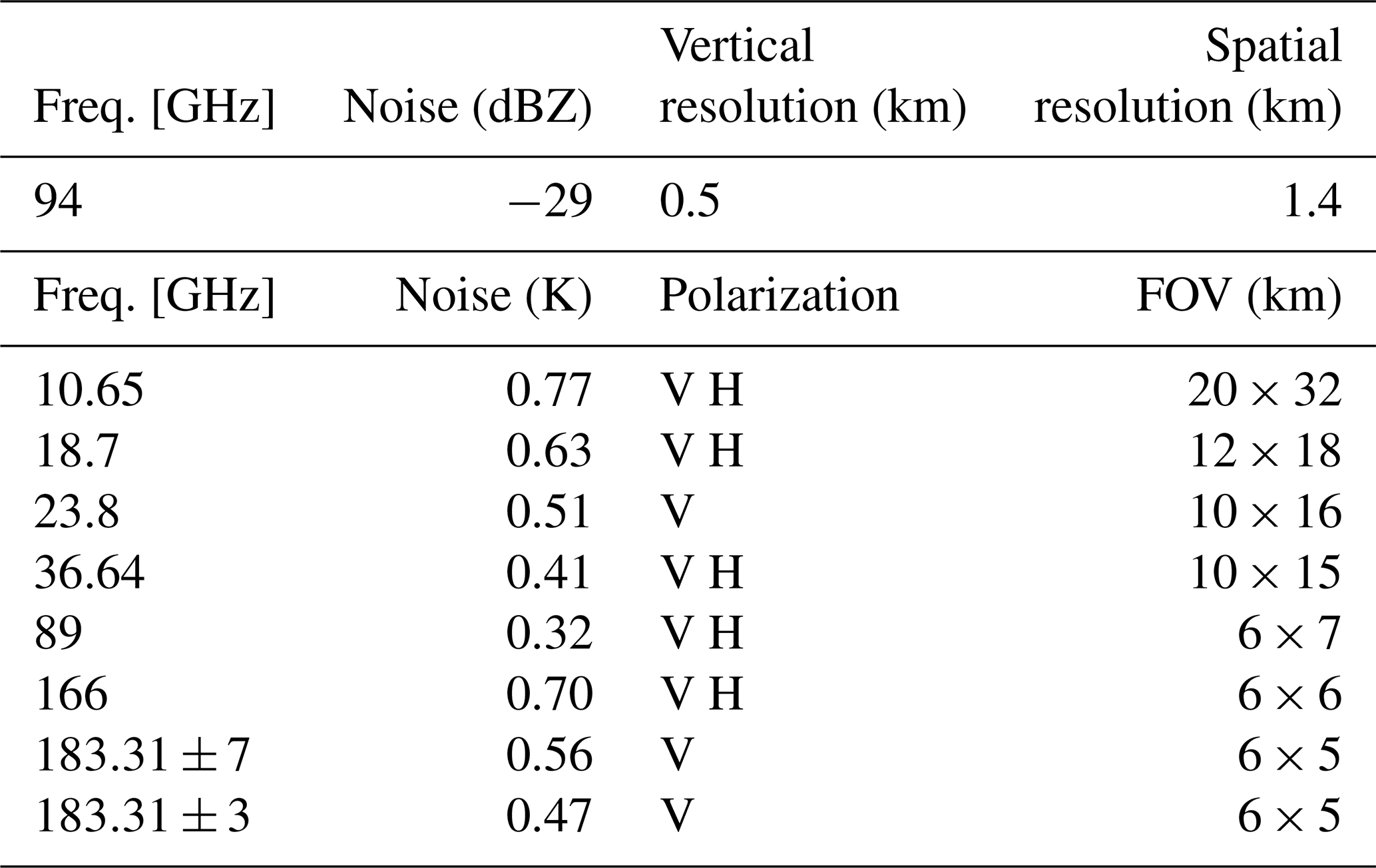
The CPR aboard the CloudSat satellite is a nadir-looking W-band radar. Table 1 outlines the specifications of the CPR. The detailed vertical structure of hydrometeors can be derived from 94 GHz radar reflectivity from the CPR. The GMI aboard the GPM core satellite is a conically scanning microwave radiometer. As shown in Table 1, the GMI channels span a wide frequency range from 10 to 183 GHz (Newell et al., 2015). In this study, brightness temperature (Tb) at frequencies of 89 GHz and higher is used since these frequencies are sensitive to the microwave scattering by frozen hydrometeors. The GMI has the highest spatial resolution among space-borne passive microwave sensors equipped with frequencies above 166 GHz. The inclined orbit of the GPM satellite has occasional orbital overlaps with polar-orbiting satellites including CloudSat, allowing for simultaneous observations at various locations from time to time.
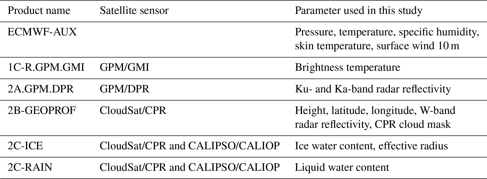
For the evaluation of the combined GMI and CPR algorithm being developed, we utilize a match-up observation dataset from GPM/GMI, Dual-frequency Precipitation Radar (DPR), and CloudSat/CPR (Turk et al., 2021). This dataset collects data when GPM and CloudSat fly over the same location within a time difference of 15 min. This dataset consists of observations from GMI, DPR, and CPR along CloudSat's ground tracks as well as the collocated ECMWF atmospheric state variable data (ECMWF-AUX). For comparison, also used are an existing cloud and precipitation product (2C-ICE and 2C-RAIN) derived from CPR and Cloud-Aerosol LIdar with Orthogonal Polarization Lidar (CALIOP) aboard the Cloud-Aerosol Lidar and Infrared Pathfinder Satellite Observations (CALIPSO) satellite (Deng et al., 2015). Detailed information regarding the products and parameters used in this study is provided in Table 2. The comparison and evaluation of the current algorithm with these datasets will be discussed in Sects. 4 and 5.
Table 2Details of the GPM, CloudSat, CALIPSO, and ECMWF-AUX products.
2.2 Cloud-resolving model
In this study, an a priori database constituted of cloud and atmospheric variables is constructed with global cloud-resolving simulations from the Nonhydrostatic ICosahedral Atmospheric Model (NICAM). The development of NICAM, initially begun by Tomita and Satoh (2004), is currently maintained by the Atmosphere and Ocean Research Institute (AORI) at the University of Tokyo, the Japan Agency for Marine-Earth Science and Technology (JAMSTEC), and the RIKEN Advanced Institute for Computational Science (RIKEN/AICS). NICAM has spawned numerous studies on tropical atmospheric dynamics (Miura et al., 2007; Miyakawa et al., 2014; Nakano et al., 2015). NICAM outputs of an Madden–Julian Oscillation (MJO) event offered a test bed for the assessment of cloud microphysical schemes in comparison with satellite observations (Masunaga et al., 2008). Technical details about the NICAM can be found in Satoh et al. (2008, 2014). The version of NICAM simulations adopted in this study was run using a single-moment microphysical scheme with a horizontal resolution of 14 km and a vertical resolution of 38 layers.
2.3 Forward model
The Joint Simulator for Satellite Sensors (J-sim) (Hashino et al., 2013, 2016) is used for forward simulations of satellite observations in this study. J-sim, being developed by Japan Aerospace Exploration Agency (JAXA), contains radar and microwave radiometer modules based on the Satellite Data Simulator Unit (SDSU) (Masunaga et al., 2010), which are employed for simulating observations compatible with GPM/GMI, DPR, and Cloud Sat/CPR. J-sim allows various microphysical assumptions to be tested, such as particle size distribution (PSD) and particle shape in the forward radiative transfer calculations (for details, see Sect. 3.1). Technical details of J-sim are described in Hashino et al. (2013, 2016).
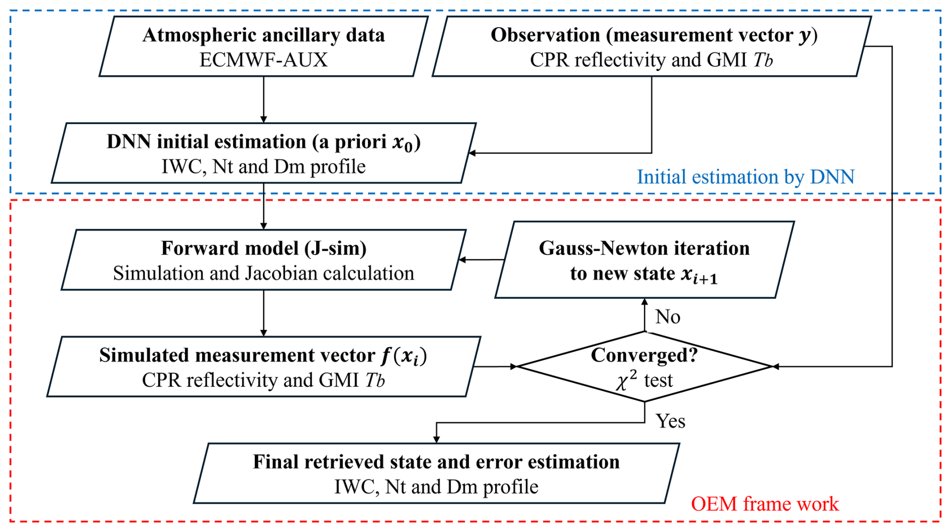
In this section, the current algorithm methodology is described to retrieve the vertical profiles of IWC, Nt, Dm, and the associated uncertainties. The algorithm flow shown in Fig. 1 consists of two components. The first component, marked by a dashed blue box, produces an initial estimation of the vertical profiles of IWC and Nt (and Dm) using a deep neural network (DNN). In the second component indicated by a dashed red box, the optimal estimation method (OEM) is adopted to optimize the frozen hydrometer profile (IWC, Nt, and Dm) using the DNN estimates as the first guess and then estimates the retrieval error. The DNN technique has the disadvantages that estimates are highly dependent on the training dataset and that uncertainty cannot be easily evaluated, but it has the advantage of obtaining reasonable estimates with a very low computational cost. The DNN technique is suitable for a quick estimation of an initial guess. On the other hand, OEM is computationally more expensive than DNN but is a well-established methodology, providing statistically robust retrievals that best match observations (Rodgers, 2000) beyond the constraint of the a priori database used for the DNN component. OEM is suitable for the final optimization of the retrieved values and the estimation of uncertainty. The cloud microphysics assumptions commonly used by DNN and OEM are described in Sect. 3.1, the details of the DNN training in Sect. 3.2, and the details of the OEM framework in Sect. 3.3; an example of retrieval using this combined algorithm is shown in Sect. 3.4.
3.1 Cloud microphysical assumption
3.1.1 Particle size distributions
The cloud PSD is determined in a complex manner depending on a variety of factors such as in-cloud temperature but needs vast simplifications in practice when formulated in retrieval algorithms. In previous studies, lognormal or gamma distribution functions (Austin et al., 2009; Deng et al., 2010), which consist of temperature-dependent PSD parameters, have been mainly used to capture the basic properties of PSD. In this study, the following temperature-dependent gamma PSD function is assumed as in Heymsfield et al. (2013):
Here N0 is the intercept, μ is the dispersion, λ is the slope parameter, and D is the maximum dimension of a particle. In this algorithm, μ is prescribed as a function of temperature (T) as defined by Eq. (2) of Heymsfield et al. (2013), while N0 and λ are free parameters to be optimized in the algorithm. The PSD for liquid hydrometeors (cloud water and rain) is as given by the NICAM cloud microphysical scheme (Tomita, 2008).
3.1.2 Particle shapes and densities
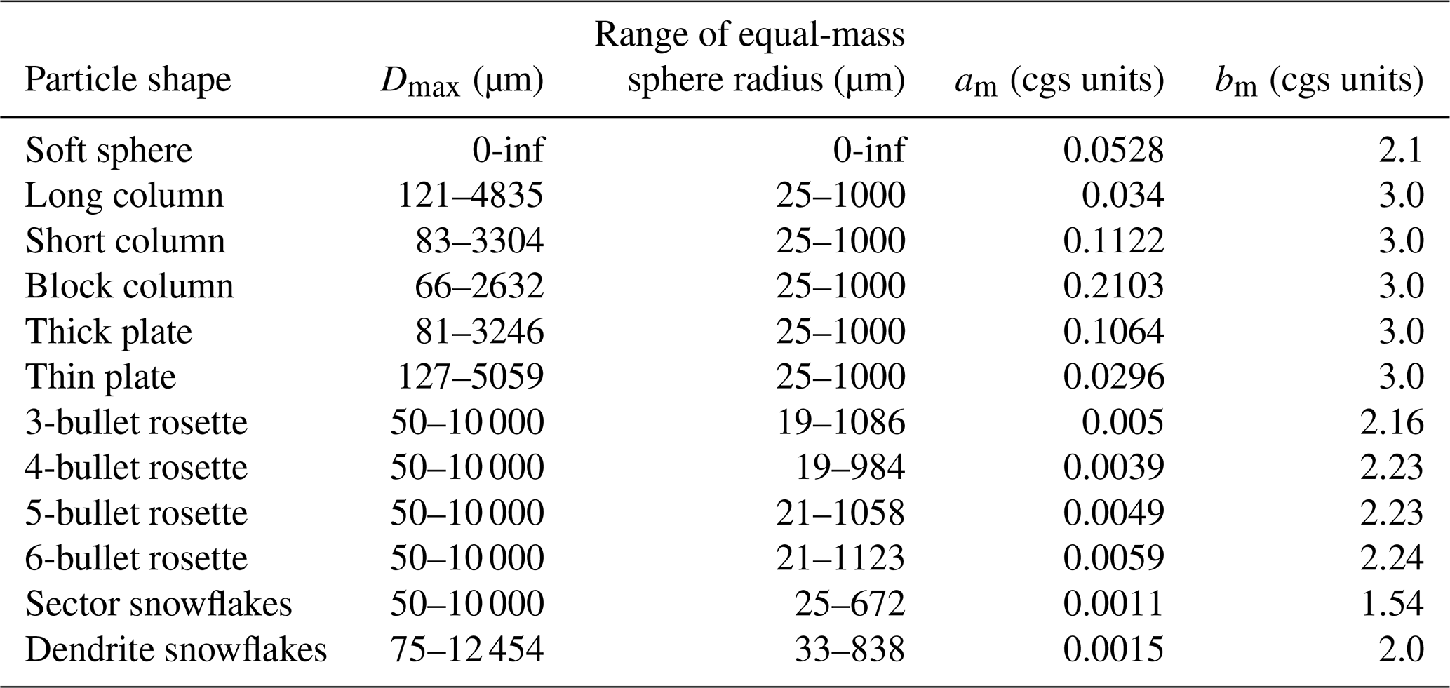
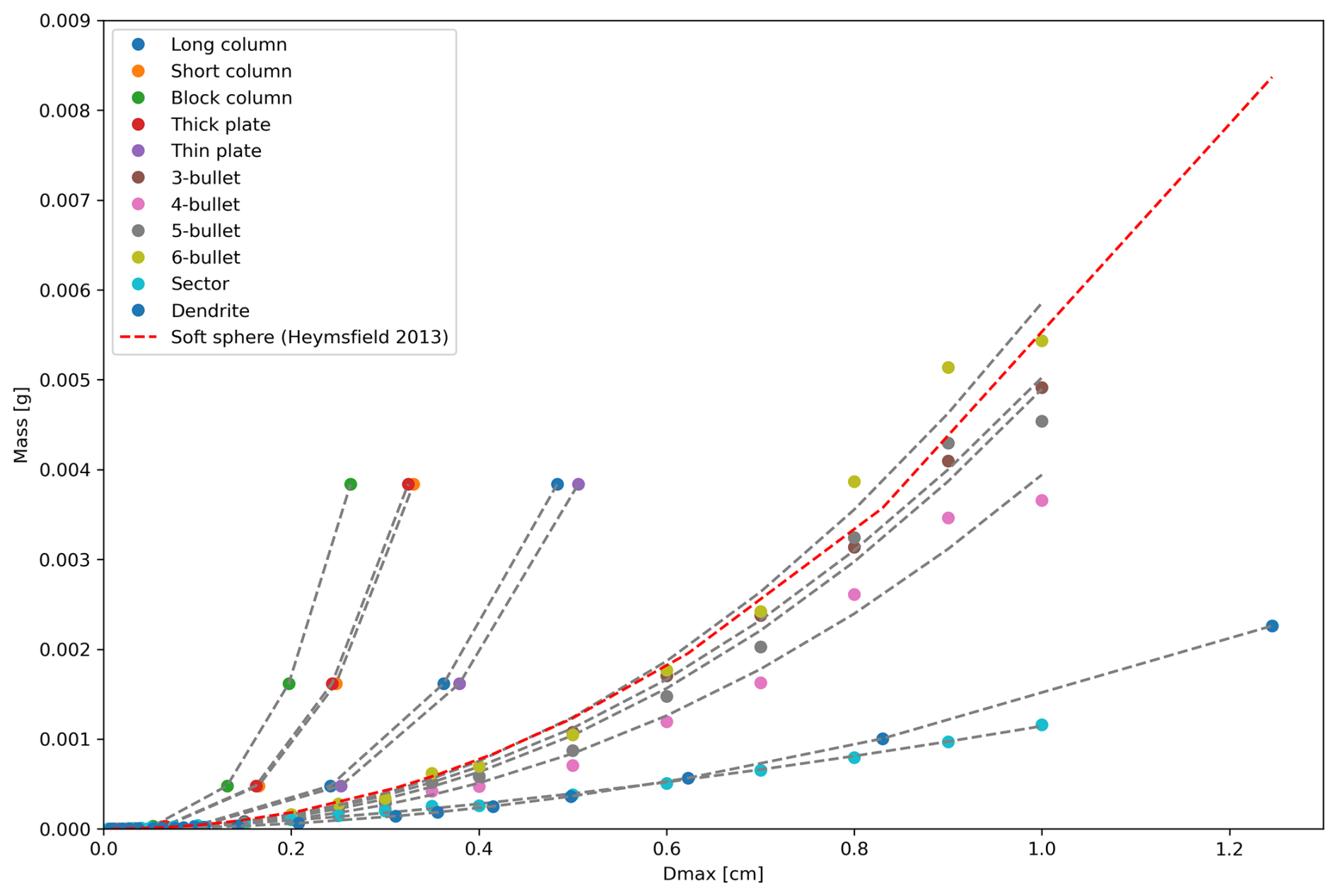
Radar and radiometric observations also depend on the shape and density of frozen hydrometeors. Frozen hydrometeors are more diverse in shape and density than liquid hydrometeors. For example, light snowflakes have a density of less than 100 kg m−3 and have significantly different single scattering properties (SSP) from spherical solid ice (with the density of 916 kg m−3). The discrete dipole approximation method (DDA) has been widely used to calculate SSP for non-spherical particles (Draine and Flatau, 1994; Liu, 2008; Okamoto, 2002). J-sim has an option to incorporate the SSPs of 11 different non-spherical shapes into radiative transfer calculations using pre-computed DDA databases (Liu, 2008). These non-spherical particle models are assumed to be randomly oriented, and the effects of ice-particle orientation on V- and H-polarized Tb (Gong and Wu, 2017) are not considered in this study. In addition to these non-spherical particle models, this algorithm assumes a “soft sphere” with the mass–diameter (m–D) relationship reported in Heymsfield et al. (2013). Figure 2 and Table 3 show the m–D relationship and the parameters of each particle model used in this study. Section 4 provides the retrieval results assuming “soft sphere” particle model, and Sect. 5 discusses the optimal particle shape assumptions including non-spherical models.
Table 3Details of the parameter for the 12 different ice-particle models.
3.1.3 Retrieval parameters
The retrieval parameters of frozen hydrometers are IWC, Nt, and Dm, as expressed by the following equations.
The definition of particle size varies among previous studies. Although Dm is used in the present algorithm, effective radius (Re) is also calculated by Eq. (5) for ease of comparison with existing data products. The parameters of area–diameter relationship aa and bb in Eq. (5) are set to the values reported in Heymsfield et al. (2013).
3.2 Deep neural network for initial value estimation
The flowchart of DNN training is shown in Fig. 3. As mentioned earlier, the frozen hydrometeor datasets of the cloud-resolving model (NICAM) are used as the reference data, and the observations simulated by the forward model (J-sim) from the NICAM data are input to the DNN training. The training dataset and procedure are described below in some detail.

3.2.1 Training dataset
Figure 4a, c, and e show the contoured frequency by altitude diagram (CFAD) of absolute humidity (AH), and temperature (T) from NICAM reference dataset in the tropics. For comparison, Fig. 4b, d, and f plot the CFAD of AH and T from the ECMWF-AUX product, respectively, for 3 winter months (DJF) of 2015 in the tropics. The tropical oceans have little seasonal variation, so there are no significant changes over different seasons. Although not shown in Fig. 4, IWC, pressure (P), liquid water content (LWC), sea surface temperature (SST), and sea surface wind speed (SSW) obtained from NICAM are also recorded for forward calculations. Figure 4e and f show the CFAD of radar reflectivity simulated from NICAM and actual observed CPR reflectivity. The humidity, temperature, and radar reflectivity simulated from NICAM are similar to those of real atmospheric profiles, indicating that NICAM serves well as a reference (a priori) database for initial value estimation.
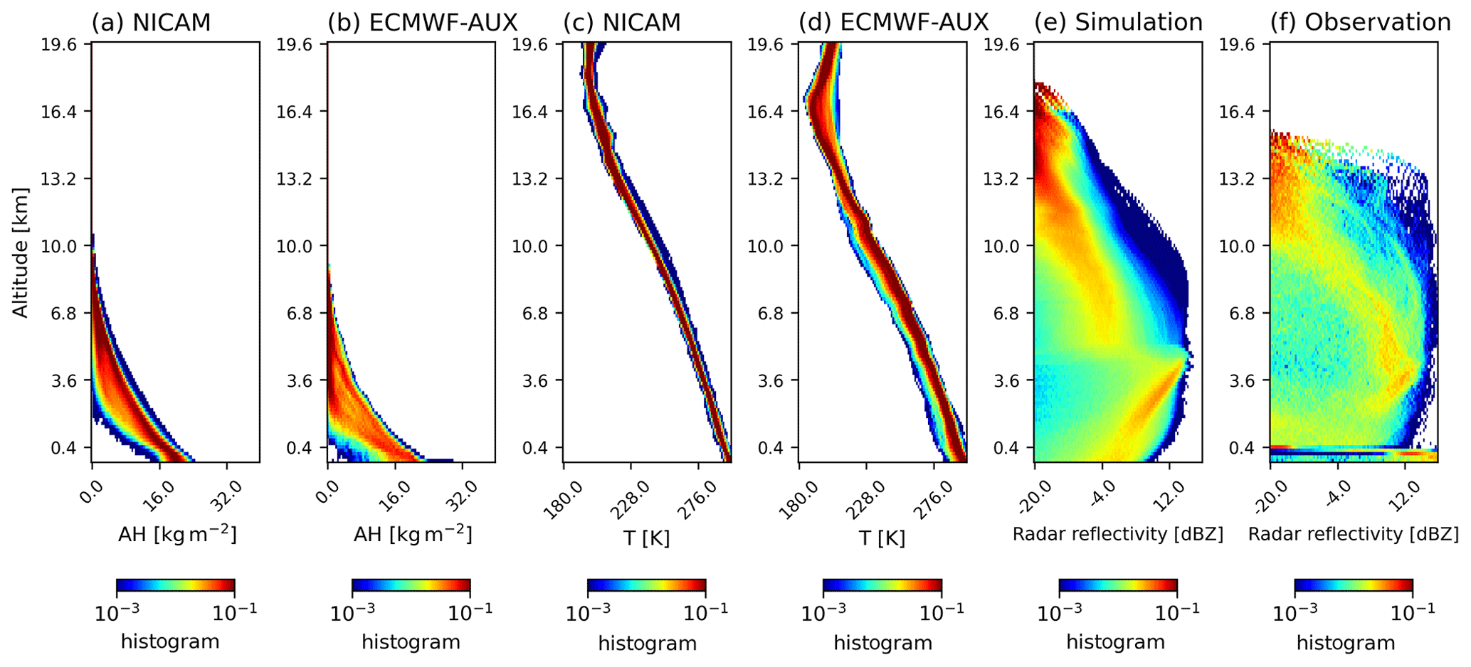
Figure 4CFAD of NICAM reference dataset and actual atmospheric variables. CFAD of temperature profiles for (a) NICAM and (b) ECMWF-AUX. CFAD of absolute humidity profiles for (c) NICAM and (d) ECMWF-AUX. CFAD of radar reflectivity profiles for (e) simulation and (f) CPR observation.
3.2.2 DNN training
The DNN transforms the input data using the weight matrix W and the activation function φ(x). Using a nonlinear function φ(x), DNN allows for a nonlinear transformation. In this study, the widely used ReLU function is adopted as φ(x). The DNN inversion model yDNN can be written as follows for input data: xi.
Here, cn values are constant vectors. The DNN model consists of three layers with 200 nodes in this study. During DNN training, W is optimized using the back-propagating algorithm to minimize the following loss function JDNN.
where the reference data yi are NICAM-based frozen hydrometer profiles, and the input data xi are the simulated observation from reference yi for GMI and CPR. Therefore, yi can be represented as the true inversion solution of the forward model F−1(xi). The DNN inversion model yDNN(xi) would ideally approach the true inversion model F−1(xi) through the minimization of JDNN. In practice, care must be taken to avoid technical issues such as overfitting.
To stabilize the DNN training, the following preprocessing of input data is performed. GMI Tb depends not only on cloud physical parameters but also on water vapor, temperature profiles, and surface emissions. To factor out these effects, ΔTb (above 89 GHz), which is the all-sky Tb minus the clear-sky Tb, is used as the input for DNN. Clear-sky Tb is obtained by repeating the forward simulations with all condensates taken out. The clear-sky Tb values for the real observations are calculated similarly but with the atmospheric states from ECMWF-AUX (see Sect. 4 for details). The CPR reflectivity profiles have a much larger number of dimensions than the GMI Tb data, which are used together as DNN inputs. An empirical orthogonal function (EOF) analysis is performed to retain only the first 10 principal components of radar reflectivity profiles (EOFZej, j=1–10), so the dimension size is made comparable between CPR and GMI observations. The cumulative variance by the top 10 principal components accounts for approximately 99.9 % of the total variance. The principal component EOFZej is obtained from the Eqs. (8) and (9).
Here, ej is the eigenvector of Eq. (8); and represent the radar reflectivity profile and its vertical average, respectively, for the nth sample in the training data; Zeobs is the observed radar reflectivity profile; and EOFZej is the jth principal component.
It is noted that the NICAM simulations contain errors due to the limited resolution of the model or the representativeness of real cloud profiles by the model. These errors would only remotely affect the final retrieval in that the DNN-derived solution is adjusted by the OEM as outlined next. As such, the role of the DNN in this algorithm is an efficient production of the initial values for the OEM component.
3.3 Optimal estimation for the final retrieval and uncertainty evaluation
The bottom half of Fig. 1 shows the main flow of the OEM for finale retrieval and uncertainty evaluation. The OEM is a Bayesian method that finds a solution which maximizes the given posteriori possibility density function ppost(X | Y) (Rodgers, 2000). Here, the state vector X is defined by combining vertical profiles of IWC and Nt, and the measurement vector Y is the CPR Ze and GMI Tb above 89 GHz.
Here, n is the number of cloud ice layers. IWC and Nt profiles are set to be in a logarithmic form to avoid negative estimates. The microwave radiative transfer at 89 GHz and higher frequencies is significantly affected by water vapor. Ideally, the water vapor profile should also be included in the state vector X of Eq. (10) and optimized within the OEM framework. From a technical perspective, however, optimizing both the ice-particle and water vapor profiles is computationally demanding, as the amount of information provided by satellite observations (i.e., the dimension of the observation vector Y in Eq. 10) is too limited relative to the number of unknown parameters to be retrieved (i.e., the dimension of the state vector X). This imbalance can cause convergence issues in the retrieval. For thick ice clouds such as deep convective clouds, scattering signals from ice particles are expected to dominate brightness temperature despite the considerable absorption and emission signals from water vapor. Therefore, the water vapor profile from ECMWF-AUX is used as a fixed input, and only the ice cloud profile is optimized. The fidelity of the ECMWF-AUX water vapor profile is discussed in Sect. 4.1.
Assuming a Gaussian possibility density function, the cost function JOEM to be minimized by OEM is written as the following equation.
where F(X) is the satellite observation simulated by the forward model (J-sim) from the state vector X; Xa is a priori state, given by the initial value estimated by DNN; and Sa is the covariance error matrix for the a priori state. For the sake of mathematical consistency, Sa in theory should be specified using error covariances calculated from the a priori dataset (i.e., the DNN training data). However, the error correlations derived from NICAM may not be fully reliable, as NICAM is a limited representation of cloud statistics in the real atmosphere. Hence Sa is tuned in a simplistic manner without referring to the a priori dataset. The elements of Sa including off-diagonal terms are defined as to take into account the level-to-level correlations (Delanoë and Hogan, 2008; Rodgers, 2000). Here, dij is the distance between k and l layers. Although several values of σa and L are tested and have little impact on the retrieval results, the combination σa=0.5 and L=3.5 km, which gives the most favorable performance, is selected. Se is the covariance error matrix for measurements which take into account not only sensor-derived measurement errors but also forward simulation-derived errors such as the uncertainty due to particle shape assumptions. The measurement error of CPR reflectivity is set to be 2.5 dBZ according to previous studies (Deng et al., 2010). A previous study (Kulie et al., 2010) reported that the uncertainty in the high-frequency Tb due to particle shape assumptions is K at 166 GHz. In addition, since the GMI footprint is larger than the CPR footprint, errors caused by the non-uniform beam filling (NUBF) effect should be considered. The measurement error of GMI Tb is set sufficiently large value of 4 K, and the off-diagonal terms of Se are assumed to be zero.
The Gauss–Newton iteration method is used as the algorithm for finding the minimum value of the cost function in Eq. (11), and the state vector of the ith iteration Xi is repeatedly updated until convergence according to the following equation:
The Jacobian matrix H is calculated using the finite difference method by applying forward simulations to IWC and Nt profiles being perturbed in each layer. The convergence is evaluated using the χ2 test (Rodgers, 2000) to obtain the final-retrieved state vector. OEM offers the retrieval errors defined by the trace of the following matrix S defined below.
It should be noted that since Sa and Se are built upon simple assumptions, the retrieval error calculated by Eq. (14) is valid only approximately.
3.4 Example of the retrieval
Figure 5 shows an example retrieval for a given CPR and GMI match-up observation. The solid black lines in Fig. 5a and b are the CPR reflectivity and GMI ΔTb used as the input, and Fig. 5c and d plot the DNN-based initial estimates of IWC and Nt profiles and the iteration process by OEM. Figure 5a also shows the CPR reflectivity and GMI ΔTb simulated by the forward model using the DNN and OEM estimates as the input. The DNN yields the estimates that are roughly, if not perfectly, consistent with the satellite observations, suggesting that the DNN performs well as an initial value estimator. The OEM, refining the DNN estimate, estimates the frozen hydrometer profiles in better agreement with both the CPR reflectivity profile and GMI Tb. A statistical evaluation of the algorithm performance will be discussed in Sects. 4 and 5.
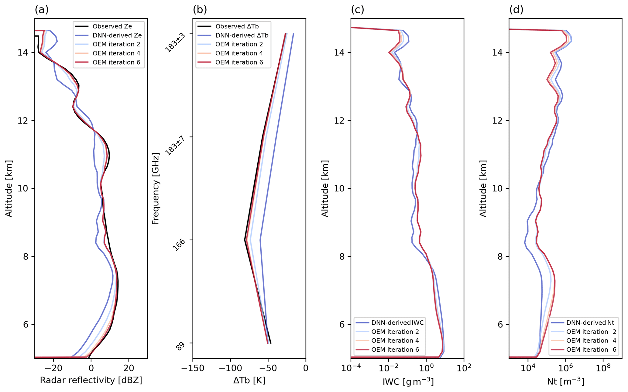
Figure 5Example of the initial estimation by DNN and iteration process by OEM. (a) The CPR reflectivity observations are plotted as a black line and radar reflectivity simulated from the DNN initial estimates as a dark-blue line. The OEM iteration process is shown with the number of iterations, and the radar reflectivity simulated from the OEM final estimates is plotted with a dark-red line. (b) Same comparison as in (a) for GMI ΔTb. (c) The DNN initial estimates of IWC are plotted with a dark-blue line and the OEM final estimates of IWC with a dark-red line. (d) Same comparison as in (c) for Nt.
4.1 Application to match-up observations of GPM and CloudSat
In this section, the present algorithm is applied to actual match-up observations from CloudSat and GPM satellites (Turk et al., 2021). Figure 6a and b show a snapshot of simultaneous observations of CPR and GMI on 18 March 2016, containing a mature tropical convective system. Observed GMI Tb is plotted with solid lines, and the simulated clear-sky Tb from atmospheric data ECMWF-AUX is plotted with dashed lines. The GMI Tb and the simulated clear-sky Tb are in good agreement in the clear-sky regions (latitudes 11°), showing the fidelity of the temperature and humidity sounding in use. A sensitivity experiment has been conducted (not shown) with the ECMWF-AUX humidity profile replaced with a saturated or supersaturated water vapor profile within the cloud-masked regions. This change was found to have no significant impact on the ice cloud retrieval results. Therefore, the ECMWF-AUX humidity profile is used as input even within cloudy regions in this study. The ΔTb for each channel is the difference between GMI Tb and simulated clear-sky Tb.
Figure 6c plots GMI 166GHz ΔTb with a dotted black line and vertically integrated CPR reflectivity Zeint, defined as follows (Kulie et al., 2010), with a blue line:
Here, HFL and HCT are the freezing level and cloud-top height, respectively. Care needs to be taken, however, when comparing Zeint with the corresponding GMI ΔTb. While the CPR is a nadir-looking radar, GMI observations have a slanted viewing angle of about 52.8° at Earth's surface. As a result, the layer of cloud ice aloft producing a depression of GMI Tb is horizontally offset from the CPR profile matched up to the surface geolocation. To reduce the error due to this misalignment, ΔTb is shifted so that the correlation of horizontal pattern between ΔTb and Zeint becomes the highest (shown in red line). As described in Sect. 3.3, the errors caused by the NUBF effect are already considered in the covariance matrix Se. The CPR reflectivity and the shifted GMI ΔTb are input to the algorithm to retrieve the frozen hydrometer profile. The retrieved IWC, Nt, and Dm profiles obtained from the current algorithm are shown in Fig. 7.
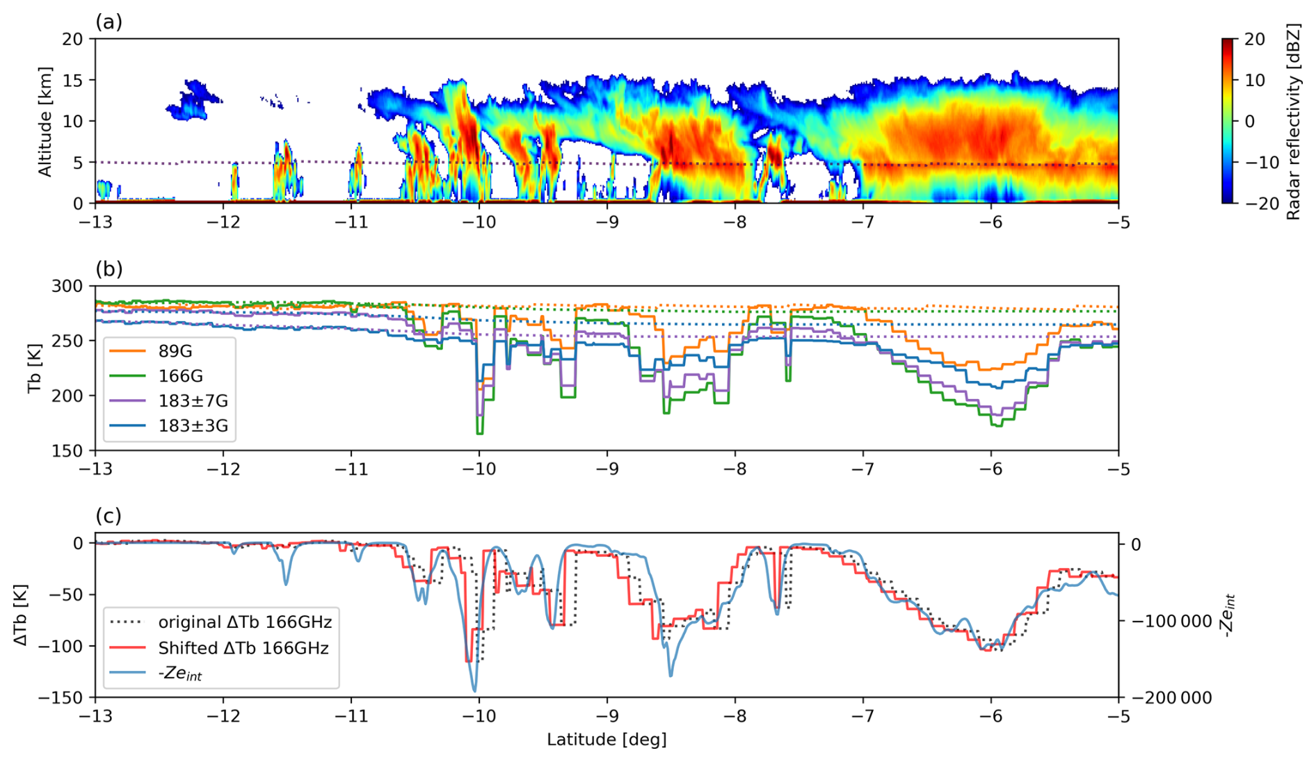
Figure 6The match-up observation data of CloudSat/CPR reflectivity and GPM/GMI brightness temperature for algorithm inputs. (a) The vertical distribution of CPR reflectivity and freezing level (dotted line). (b) The solid lines are GMI Tb observations, and the dotted lines are the clear-sky brightness temperature simulated from ECMWF-AUX. (c) Horizontal distribution of CPR Zeint (red line), 166 GHz ΔTb (black line), and shifted 166 GHz ΔTb (blue line).
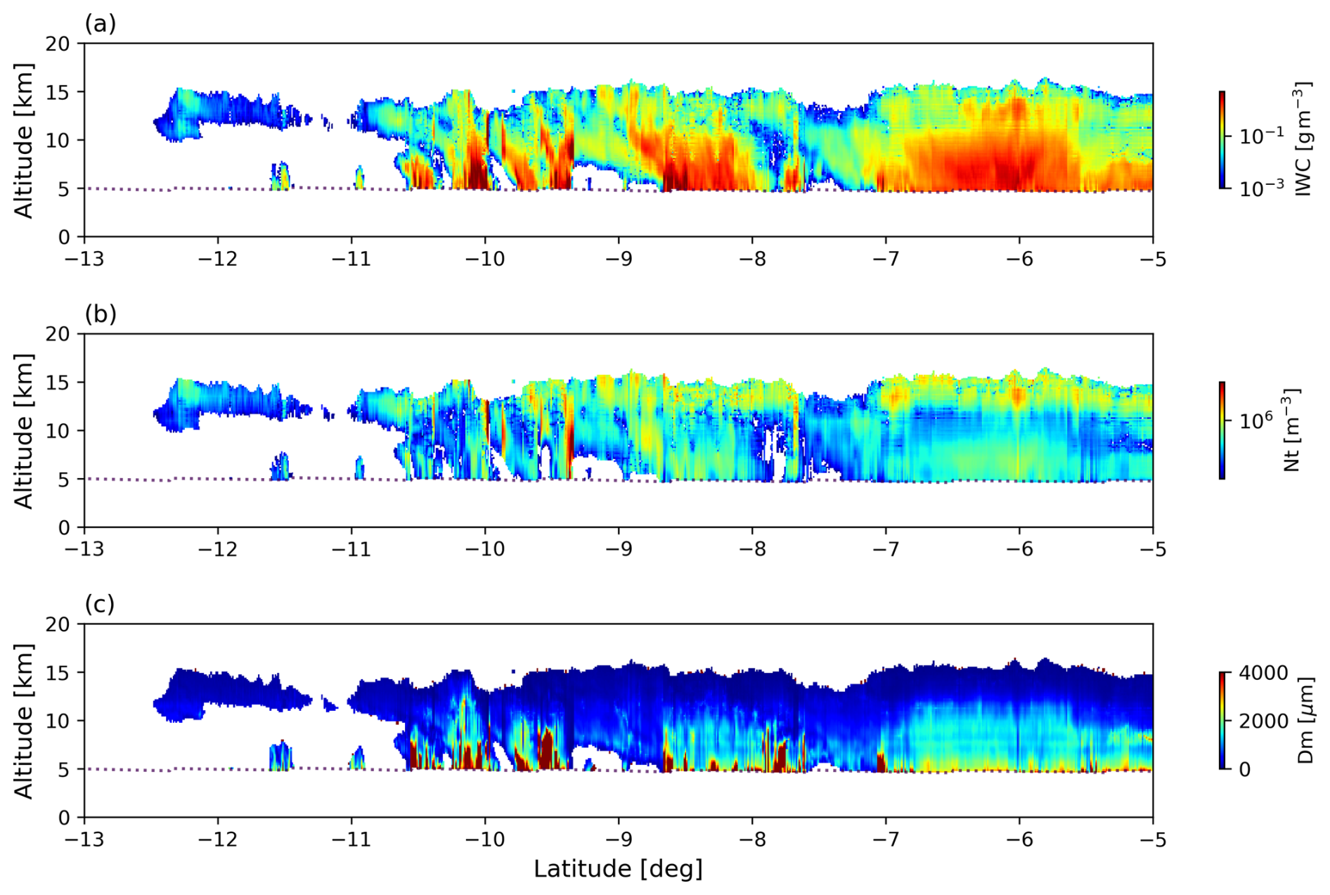
Figure 7The retrieved IWC (a), Nt (b) and Re (c) profiles from the current algorithm. The dotted lines are the freezing level.
4.2 Reduction of uncertainty by synergy between GMI and CPR observations
The OEM also provides the retrieval errors by Eq. (14). Figure 8a and b show the retrieval error of IWC and Nt on the logarithmic scale. Figure 8c and f are example profiles of the IWC and Nt retrieval errors extracted from a latitude of −6°. To assess the performance of the GMI-CPR synergy, the retrieval errors are compared between the CPR-only (blue line) and combined-use cases (red line), respectively. The combined-use case has smaller errors than the CPR-only case in all layers, confirming a positive impact of adding GMI observations to CPR measurements.
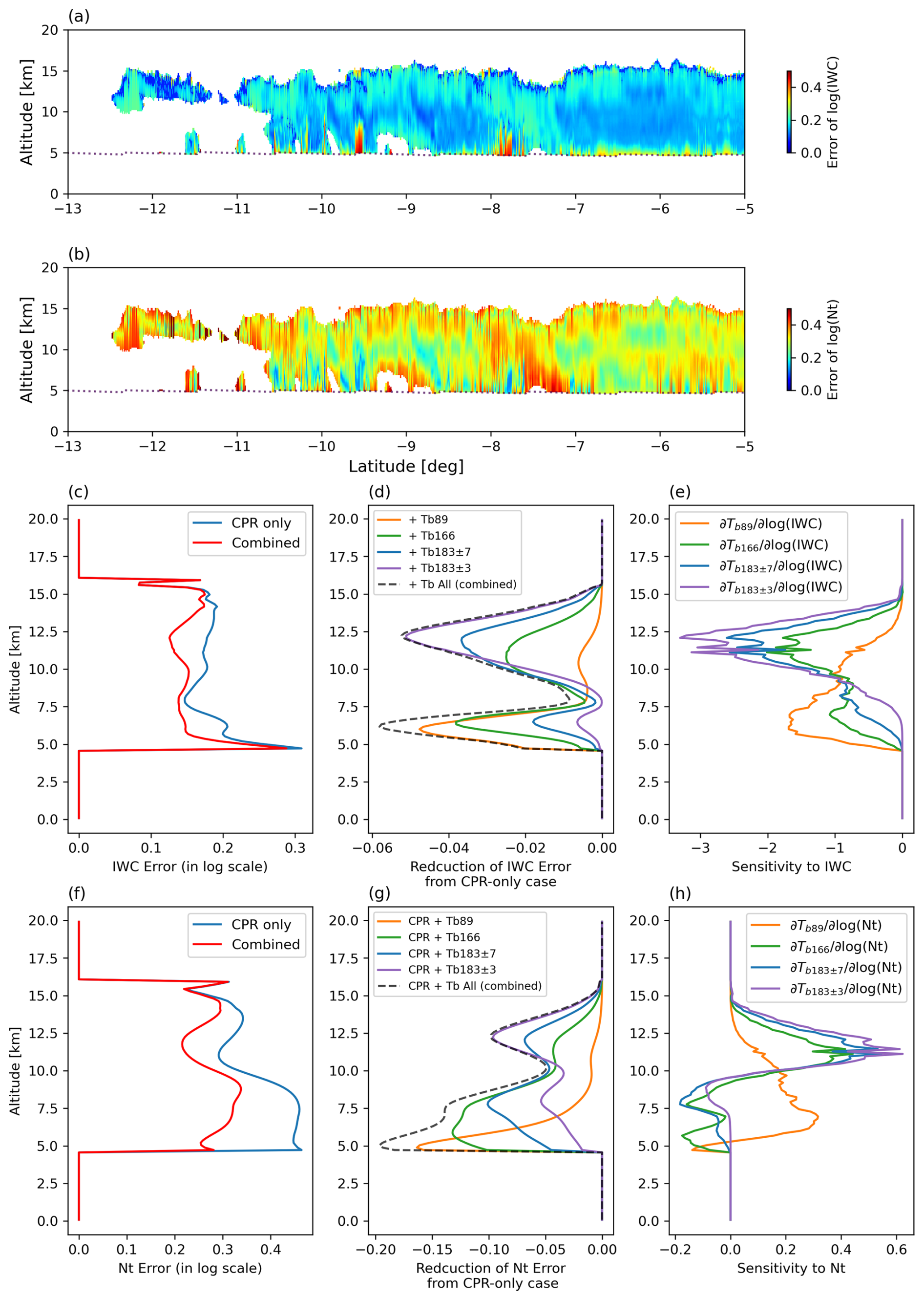
Figure 8Retrieval error analysis for investigation of synergy between CPR and GMI observations. Retrieval error profiles of (a) IWC and (b) Nt on a logarithmic scale. (c) An example of IWC error profiles calculated for CPR-only (blue line) and combined-use case (red line). (d) Error reductions of IWC from the CPR-only case by adding each GMI high-frequency channel to the CPR observation. (e) Sensitivity (Jacobian) of each GMI high-frequency channel to IWC in each layer. (f) Same comparison as in (c) for Nt. (g) Same comparison as in (d) for Nt. (h) Same comparison as in (e) for Nt.
Figure 8d and g plot the reduction of errors when each GMI channel is added to the CPR-only observation one by one. The 89 GHz Tb contributes mainly to the reduction of retrieval errors in the lower layers, while 183±3 GHz Tb mainly reduce errors in the upper layers. The error reduction in the upper layers is exclusively owing to 183±3 GHz Tb only, with the contribution of other frequencies being minimal. The 166 and 183±7 GHz Tb contributes across all layers from the upper to the lower layers. Figure 8e and h show the sensitivity of each GMI high-frequency channel to IWC and Nt in each layer using the Jacobian matrix in Eq. (13). The peak of error reduction shown in Fig. 8d and g is consistent with the peak of sensitivity shown in Fig. 8e and h for each channel. As noted earlier, the true values of Sa and Se are unknown, so the retrieval errors theoretically calculated by Eq. (14) may not be accurate in practice. Given the uncertainty in Sa and Se, the quantitative interpretation of error reductions in Fig. 8 requires caution. Nevertheless, the sensitivity analysis results in Fig. 8d, e, g, and h meet physical expectations, and thus the error estimates above are considered to be valid from a qualitative perspective.
5.1 Reproducibility of CPR and GMI observations
In situ data to validate cloud physical parameters are limited in availability. The algorithm performance is therefore tested using measurables (Ze and Tb) instead of retrieved variables (IWC, Nt, and Dm). To this end, measurables are reproduced with forward simulations using the retrieved frozen hydrometer parameters as the input for comparison with actual observations. This comparison is performed using 10 match-up observations of CPR and GMI, including the case shown in Figs. 6 and 7. The 2C-RAIN product is used for cloud liquid water and rain water beneath the cloud-ice layer. As far as the layer of liquid cloud and rain is optically thick for microwave radiation as typical of heavily raining clouds, high-frequency Tb becomes far less sensitive to liquid water path (LWP) than to IWP (Masunaga, 2022), and the uncertainty resulting from the liquid component is negligible.
Figure 9a and b show an example of simulated CPR radar reflectivity in the solid-phase layer and GMI Tb from the current algorithm estimates. Compared to the actual observation shown in Fig. 6, the spatial structure of radar reflectivity and the horizontal distribution of Tb are reproduced well. Figure 9c and d are scatter plots of the simulated and actual observations for the 10 match-up cases. The simulated radar reflectivity and Tb at high-frequency channels are both unbiased overall against the actual observations. This result assures self-consistency of the current algorithm.
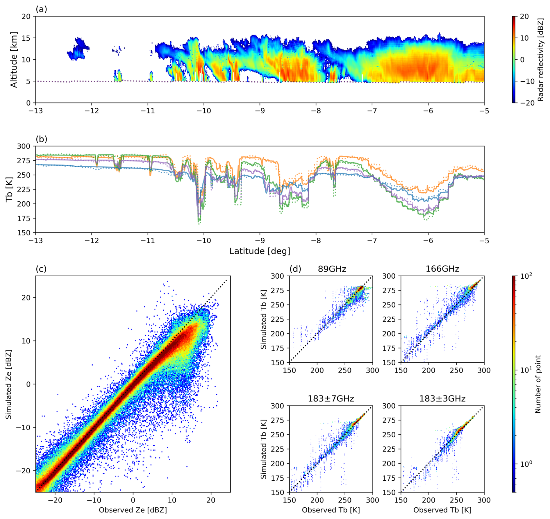
Figure 9Reproducibility of the CPR reflectivity and GMI Tb for the current algorithm. (a) Example of the simulated CPR reflectivity and (b) simulated GMI Tb (solid lines) from the frozen hydrometeors estimated by the current algorithm. Dotted lines are actual GMI Tb observations for comparison. (c) Statistical comparison between actual reflectivity and simulated reflectivity for 10 match-up cases. (d) Results of the same comparisons as in (c) for each GMI high-frequency channel.
5.2 Reproducibility of DPR observations
DPR carried by the GPM core observatory yields simultaneous observations with GMI radiometry, providing additional data to assess the algorithm performance. GPM/DPR, a suite of Ku- and Ka-band radars, are sensitive to large frozen hydrometeors such as snow and graupel inside of deep convective clouds, having information independent of CPR and GMI observations. This study uses DPR reflectivity above freezing level to test the cloud ice estimates from the present algorithm. Similarly to Fig. 9, the Ku- and Ka-band radar reflectivity is simulated from the current algorithm estimates of frozen hydrometers (Fig. 10b and d) for comparison with the actual DPR observations ((a) and (c)). The current estimates of cloud ice reproduce the overall distribution of observed Ku and Ka radar reflectivity. As shown in Fig. 10e and f, the simulated DPR reflectivity exhibits no systematic bias against the actual DPR observation for the 10 match-up cases despite the significant spread.
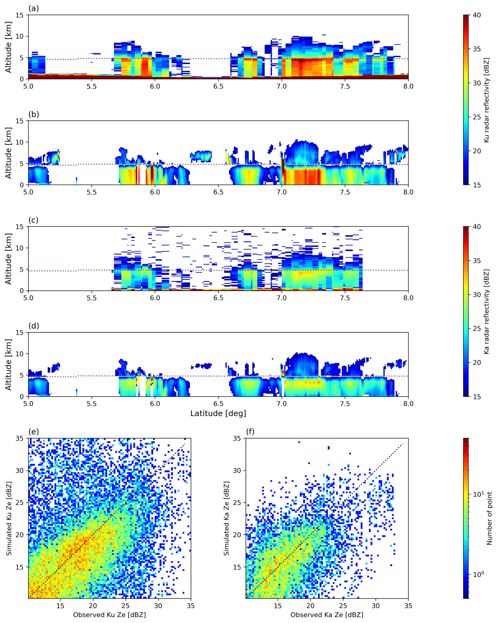
Figure 10Reproducibility of DPR Ku and Ka-band radar reflectivity. Snapshot of the (a) Ku-DPR observation and (b) simulated Ku-band reflectivity from the current algorithm estimates. Snapshot of the (c) Ka-DPR observation and (d) simulated Ka-band reflectivity from the current algorithm estimates. (e) Statistical comparison between actual Ku-DPR observations and simulated Ku-band reflectivity using 10 match-up cases. (f) Same comparison as in (e) for Ka-band reflectivity.
5.3 Particle shape assumptions
This section discusses the assumptions of the particle model optimal for this synergistic algorithm. CPR reflectivity mainly captures the backscattering properties of particles, while GMI Tb values mainly observe the scattering and absorption properties. A combined use of these two independent information has the potential to constrain uncertainties in the assumptions of the particle model. To test this, the reproducibility of CPR and GMI observations is evaluated with different non-spherical particle models listed in Table 3. Only the particle model that consistently represents all the backscattering, absorption, and scattering properties would allow the algorithm to find the solution (frozen hydrometer profile) that accords with both CPR and GMI observations. Figure 11a–f compare the simulated reflectivity and Tb with the actual CPR and GMI observations for the six representative particle models (long column, thin plate, 4-bullet rosette, sector snowflake, dendrite snowflake and soft sphere). The CPR reflectivity is well reproduced regardless of the particle model assumptions by optimizing IWC and Nt (that is, the PSD parameters λ and N0) in our algorithm. On the other hand, the simulated Tb is clearly lower than the observed Tb for cold Tb values, except for the dendrite snowflake and soft sphere cases. These results indicate two points: (1) the soft sphere and dendrite snowflake are the optimal particle models for cold Tb values among the six models tested here, and (2) CPR observations alone are not sufficient to simultaneously constrain the uncertainties in the PSD and particle models.
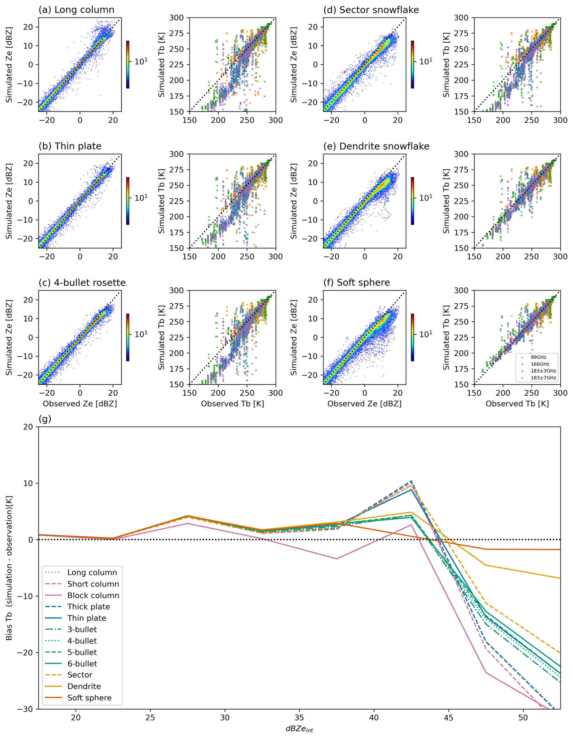
Figure 11Comparison of the reproducibility of CPR and GMI observations for various particle models. Scatter plots between actual observations and simulated observations assuming (a) long column, (b) thin plate, (c) 4-bullet rosette, (d) sector snowflake, (e) dendrite snowflake, and (f) soft sphere. (g) Dependency of Tb bias (simulation − observation) of Zeint (IWP) for each particle model.
Figure 11g plots the difference between the simulated and actual Tb as a function of IWP for each particle model assumption. Since the IWP estimate varies with the particle model assumptions, the horizontal axis is substituted by Zeint in Eq. (15). Simulated Tb is much lower than the observation for most non-spherical particle models at large Zeint (IWP), whereas for the dendrite snowflake and soft sphere, Tb bias is relatively small for the whole range of Zeint. The findings imply that for clouds with very large IWP such as deep convective clouds, the dendrite snowflake and soft sphere may be the most appropriate particle models. It should be noted, however, that for more frequently occurring clouds with moderate to low IWP, differences in Tb bias among particle models are small, making it difficult to identify a clearly preferable model. A previous study (Fig. 11 in Kulie et al., 2010) shows a similar figure to Fig. 11g and also reported that most non-spherical particle models except the dendrite snowflake exhibit excessive scattering (negative biases to actual observation) for large IWPs. Kulie et al. (2010) first converted CPR reflectivity to IWC, assuming Liu's non-spherical model (Liu, 2008), and then simulated Tb from this IWC, assuming the same particle model to compare with the actual SSMIS 157 GHz Tb. Their study assumed a fixed PSD when simulating Tb, so the failure to reproduce SSMIS Tb values may be caused by an inappropriate PSD assumption rather than the particle model. However, even our algorithm, which optimizes PSD parameters by OEM, cannot find the solution that is simultaneously consistent with the CPR and GMI observations for non-spherical particle model except for dendrite snowflake.
While the results in Fig. 11g indicate that the soft sphere assumption best reproduces satellite observations, several previous studies have reported that non-spherical particles are essential in reproducing realistic scattering signals instead of soft sphere particles (Ekelund et al., 2020; Kuo et al., 2016; Olson et al., 2016; Kulie et al., 2010). This apparent inconsistency may be explained by a few possible hypotheses as follows.
The validity of soft spheres may vary largely with the particle density model (m–D relation) in use. The present work adopts the m–D relationship from Heymsfield et al. (2013), which is different from the soft sphere model used in previous studies. The current finding does not imply that all soft sphere models, if any, are superior to non-spherical particle models used in previous studies.
The soft sphere model best fits observations for very large IWPs, suggesting that it may only be well suited for certain cloud types such as deep tropical convective clouds. This is physically reasonable because an appreciable amount of graupel is formed by riming in deep convection. The scattering properties of graupel are likely better approximated by soft spheres than snowflakes and ice crystals. In contrast, the soft sphere assumption may be less appropriate for stratiform precipitation investigated in Olson et al. (2016), where scattering is likely dominated by aggregated snow particles. Such differences in cloud microphysics between convective and stratiform clouds may explain the contrasting results between the present and previous studies.
The current retrieval is compared with the CloudSat/CALIPSO standard radar/lidar product (2C-ICE). Figure 12a and b show the IWC and Re estimates of 2C-ICE, and the observable areas for the CALIPSO lidar (lidar cloud mask above 25 %) are shaded in grey. Figure 12c and d compare the 2C-ICE estimates with the current algorithm assuming soft sphere for the 10 match-up cases. Here, Re is calculated using Eq. (5). The IWC estimates of current algorithm agree very well with 2C-ICE, but there is a positive bias in Re. In particular, the Re bias tends to increase with Re toward deep inside the cloud layer. As shown in Fig. 12a and b, in the 2C-ICE product, the combined radar and lidar observations are limited to near the cloud tops, so the retrieval in deeper cloud layers is almost based on the CPR observations only. On the other hand, this study also uses GMI, allowing synergetic observations even deep inside of clouds (as shown in Fig. 8e and h). The current algorithm actually captures large snow and graupel particles inside convective clouds, to which the DPR is sensitive (as shown in Fig. 10). In addition, lidar is sensitive to small particles, whereas microwave instruments are sensitive only to relatively large hydrometers. One possible reason for the Re bias is the difference in the sensor-specific sensitivity. Other factors could be differences in the cloud microphysical assumptions such as PSD and particle shape.
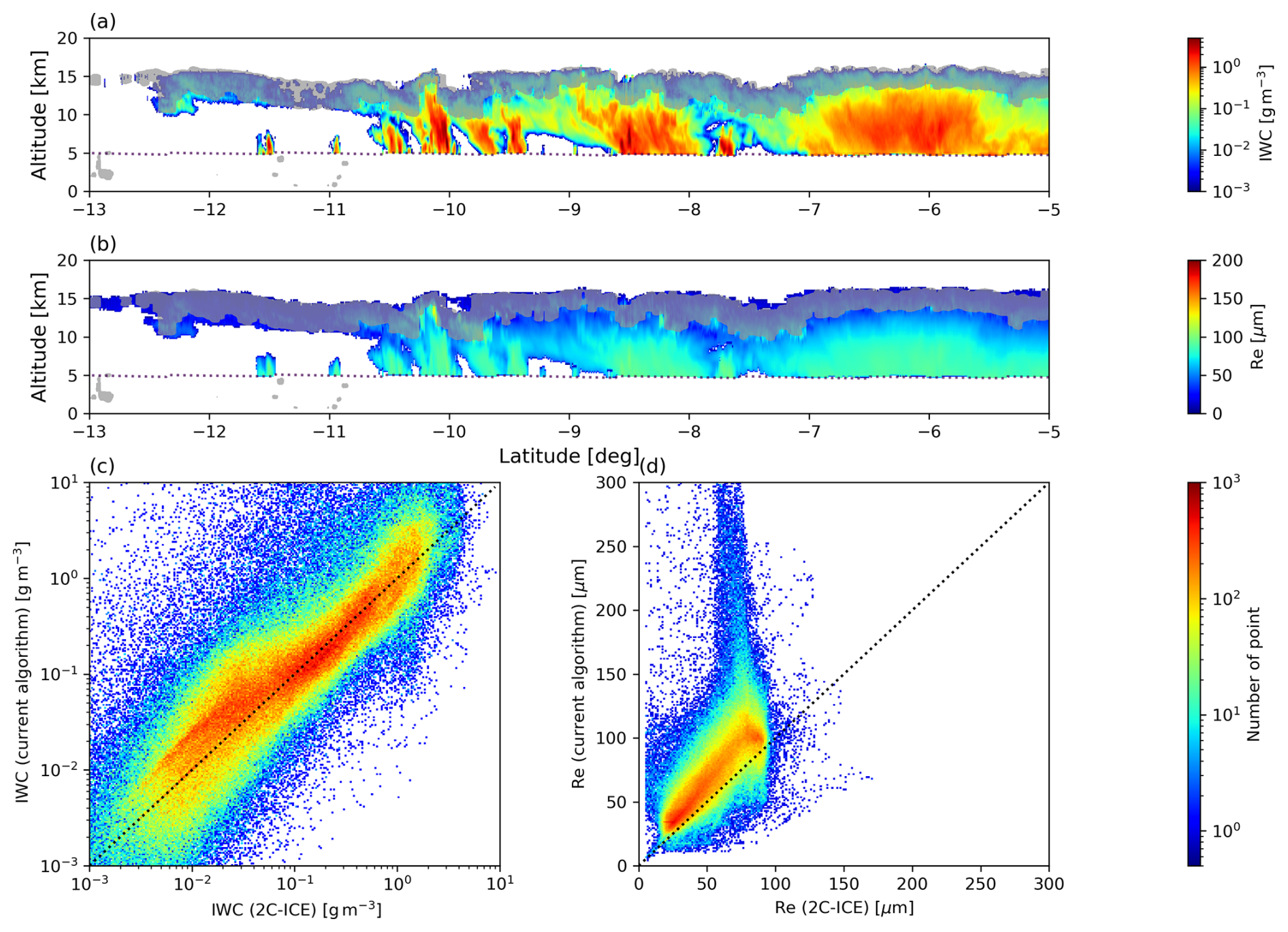
Figure 12(a) Example of IWC and Re profiles of 2C-ICE product in same case as Figs. 6 and 7. (b) Comparison of IWC and Re between 2C-ICE and the current estimates assuming soft sphere for 10 match-up cases.
This study develops an algorithm to retrieve the vertical profiles of IWC, Nt, and Dm in deep convective systems using simultaneous CPR and GMI observations. A new algorithm that combines the DNN and OEM for the inversion problem solver is proposed. The role of DNN in this algorithm is to estimate near-optimal initial values at low computational cost. The DNN is trained using an a priori database constructed from the cloud-resolving model (NICAM) (Fig. 4). The OEM uses the DNN estimate as an initial state to further optimize the frozen hydrometer profile to be consistent with CPR and GMI observations (Fig. 5). The retrieval error is calculated as a byproduct of the OEM at the in same time. The retrieval performance of the current algorithm is evaluated using match-up observations of CPR and GMI (Figs. 6 and 7). The combined use of CPR and GMI reduces the retrieval error compared to the case using CPR only, indicating a positive impact of the synergy between CPR and GMI observations (Fig. 8c and f). These reductions of retrieval error are significant at multiple altitudes where the GMI high-frequency Tb is most sensitive to ice particles (Fig. 8d, e, g, and h).
To evaluate the validity of the current algorithm estimates, the reproducibility of microwave Tb and radar reflectivity is tested through forward simulations. The CPR and GMI observations are reproduced to a reasonable extent overall (Fig. 9). Furthermore, the current estimates statistically reproduce the DPR observations (Ku- and Ka-bands), which have independent information and are sensitive to large snow and graupel particles inside convective clouds (Fig. 10). In addition, it was found that the evaluations of the simultaneous reproducibility of CPR reflectivity and GMI Tb values can constrain the choice of non-spherical particle model. For dendrite snowflake and Heymsfield's soft sphere, Tb bias is relatively small regardless of IWP, whereas the simulated Tb is much lower than observed Tb at large IWP for other particle models tested (Fig. 11).
Finally, the current estimates are compared with the existing radar–lidar cloud ice product (2C-ICE) (Fig. 12). The results are statistically in agreement for IWC, but Re tends to be overestimated by the current algorithm compared to 2C-ICE. The biases may be caused by differences in cloud microphysics assumptions (such as particle models) and the sensitivity of the sensors used in the algorithm.
The framework of the algorithm developed in this study can be applied to the combined use of various cloud/precipitation radars and millimeter/submillimeter radiometers by adjusting the sensor configuration of the forward model. In the future, we plan to extend the algorithm to Doppler CPR carried by the EarthCARE satellite and millimeter/submillimeter-wave radiometers such as GOSAT-GW/AMSR3 and MetOp-SG/ICI, which are to be launched within the next few or several years.
Code is available upon request.
The match-up observation datasets from GPM/GMI and CloudSat/CPR are included in Turk et al. (2021). The forward model used in this study (Joint Simulator for Satellite Sensors) is available from https://www.eorc.jaxa.jp/theme/Joint-Simulator/userform/js_userform.html (Hashino et al., 2013, 2016). The NICAM data used in this work will be made available upon request by the authors. The Tensorflow module in Python is used for machine learning (deep neural network).
The supplement related to this article is available online at https://doi.org/10.5194/amt-18-4791-2025-supplement.
All coding, analysis, and writing of the first draft of this study were performed by KO. The study design, discussions on results, and manuscript improvement were greatly assisted by HM.
The contact author has declared that neither of the authors has any competing interests.
Publisher’s note: Copernicus Publications remains neutral with regard to jurisdictional claims made in the text, published maps, institutional affiliations, or any other geographical representation in this paper. While Copernicus Publications makes every effort to include appropriate place names, the final responsibility lies with the authors.
Guosheng Liu and Tempei Hashino are gratefully acknowledged for making the non-spherical scattering database publicly available and helping us use it in the forward model (Joint Simulator for Satellite Sensors). The authors thank Kentaro Suzuki for providing the data of cloud-resolving model (NICAM) for our research.
This paper was edited by Pavlos Kollias and reviewed by two anonymous referees.
Austin, R. T., Heymsfield, A. J., and Stephens, G. L.: Retrieval of ice cloud microphysical parameters using the CloudSat millimeter-wave radar and temperature, J. Geophys. Res., 114, D00A23, https://doi.org/10.1029/2008jd010049, 2009.
Deeter, M. N. and Evans, K. F.: A Novel Ice-Cloud Retrieval Algorithm Based on the Millimeter-Wave Imaging Radiometer (MIR) 150- and 220-GHz Channels, J. Appl. Meteorol. Climatol., 39, 623–633, https://doi.org/10.1175/1520-0450-39.5.623, 2000.
Delanoë, J. and Hogan, R. J.: A variational scheme for retrieving ice cloud properties from combined radar, lidar, and infrared radiometer, J. Geophys. Res., 113, D07204, https://doi.org/10.1029/2007JD009000, 2008.
Delanoë, J. and Hogan, R. J.: Combined CloudSat-CALIPSO-MODIS retrievals of the properties of ice clouds, J. Geophys. Res., 115, D00H29, https://doi.org/10.1029/2009JD012346, 2010.
Deng, M., Mace, G. G., Wang, Z., and Okamoto, H.: Tropical Composition, Cloud and Climate Coupling Experiment validation for cirrus cloud profiling retrieval using CloudSat radar and CALIPSO lidar, J. Geophys. Res., 115, D00J15, https://doi.org/10.1029/2009JD013104, 2010.
Deng, M., Mace, G. G., Wang, Z., and Berry, E.: CloudSat 2C-ICE product update with a new Ze parameterization in lidar-only region, J. Geophys. Res., 120, 12198–12208, https://doi.org/10.1002/2015jd023600, 2015.
Draine, B. T. and Flatau, P. J.: Discrete-dipole approximation for scattering calculations, J. Opt. Soc. Am. A Opt. Image Sci. Vis., 11, 1491–1499, https://doi.org/10.1364/JOSAA.11.001491, 1994.
Duncan, D. I. and Eriksson, P.: An update on global atmospheric ice estimates from satellite observations and reanalyses, Atmos. Chem. Phys., 18, 11205–11219, https://doi.org/10.5194/acp-18-11205-2018, 2018.
Ekelund, R., Eriksson, P., and Pfreundschuh, S.: Using passive and active observations at microwave and sub-millimetre wavelengths to constrain ice particle models, Atmos. Meas. Tech., 13, 501–520, https://doi.org/10.5194/amt-13-501-2020, 2020.
Eliasson, S., Buehler, S. A., Milz, M., Eriksson, P., and John, V. O.: Assessing observed and modelled spatial distributions of ice water path using satellite data, Atmos. Chem. Phys., 11, 375–391, https://doi.org/10.5194/acp-11-375-2011, 2011.
Evans, K. F., Wang, J. R., Racette, P. E., Heymsfield, G., and Li, L.: Ice cloud retrievals and analysis with the compact scanning submillimeter imaging radiometer and the cloud radar system during CRYSTAL FACE, J. Appl. Meteor, 44, 839–859, https://doi.org/10.1175/JAM2250.1, 2005.
Evans, K. F., Wang, J. R., O'C Starr, D., Heymsfield, G., Li, L., Tian, L., Lawson, R. P., Heymsfield, A. J., and Bansemer, A.: Ice hydrometeor profile retrieval algorithm for high-frequency microwave radiometers: application to the CoSSIR instrument during TC4, Atmos. Meas. Tech., 5, 2277–2306, https://doi.org/10.5194/amt-5-2277-2012, 2012.
Gong, J. and Wu, D. L.: Microphysical properties of frozen particles inferred from Global Precipitation Measurement (GPM) Microwave Imager (GMI) polarimetric measurements, Atmos. Chem. Phys., 17, 2741–2757, https://doi.org/10.5194/acp-17-2741-2017, 2017.
Hartmann, D. L. and Berry, S. E.: The balanced radiative effect of tropicalanvil clouds, J. Geophys. Res.-Atmos., 122, 5003–5020, https://doi.org/10.1002/2017JD026460, 2017.
Hashino, T., Satoh, M., Hagihara, Y., Kubota, T., Matsui, T., Nasuno, T., and Okamoto, H.: Evaluating cloud microphysics from NICAM against CloudSat and CALIPSO [code], J. Geophys. Res., 118, 7273–7292, https://doi.org/10.1002/jgrd.50564, 2013.
Hashino, T., Satoh, M., Hagihara, Y., Kato, S., Kubota, T., Matsui, T., Nasuno, T., Okamoto, H., and Sekiguchi, M.: Evaluating Arctic cloud radiative effects simulated by NICAM with A-train [code], J. Geophys. Res., 121, 7041–7063, https://doi.org/10.1002/2016JD024775, 2016.
Heidinger, A. K. and Pavolonis, M. J.: Gazing at Cirrus Clouds for 25 Years through a Split Window. Part I: Methodology, J. Appl. Meteor. Climatol., 48, 1100–1116, https://doi.org/10.1175/2008JAMC1882.1, 2009.
Heymsfield, A. J., Schmitt, C., and Bnsemer, A.: Ice cloud particle size distributions and pressure-dependent terminal velocities from in situ observations at temperatures from 0 to 86 C, J. Atmos. Sci., 70, 4123–4154, https://doi.org/10.1175/JAS-D-12-0124.1, 2013.
IPCC: Climate Change 2021: The Physical Science Basis. Cambridge University Press, 2391 pp., https://doi.org/10.1017/9781009157896, 2021.
Kulie, M. S., Bennartz, R., Greenwald, T. J., Chen, Y., and Weng, F.: Uncertainties in Microwave Properties of Frozen Precipitation: Implications for Remote Sensing and Data Assimilation, J. Atmos. Sci., 67, 3471–3487, https://doi.org/10.1175/2010JAS3520.1, 2010.
Kuo, K.-S., Olson, W. S., Johnson, B. T., Grecu, M., Tian, L., Clune, T. L., Aartsen, B. H. V., Heymsfield, A. J., Liao, L., and Meneghini, R.: The Microwave radiative properties of falling snow derived from nonspherical ice particle models. Part I: An extensive database of simulated pristine crystals and aggregate particles, and their scattering properties, J. Appl. Meteorol. Clim., 55, 691–708, https://doi.org/10.1175/jamc-d-15-0130.1, 2016.
Liu, G.: A Database of Microwave Single-Scattering Properties for Nonspherical Ice Particles, B. Am. Meteorol. Soc., 89, 1563–1570, https://doi.org/10.1175/2008BAMS2486.1, 2008.
Luo, Z. and Rossow, W. B.: Characterizing Tropical Cirrus Life Cycle, Evolution, and Interaction with Upper-Tropospheric Water Vapor Using Lagrangian Trajectory Analysis of Satellite Observations, J. Climate, 17, 4541–4563, https://doi.org/10.1175/3222.1, 2004.
Masunaga, H.: Satellite Measurements of Clouds and Precipitation, Springer Nature Singapore, 297 pp., https://doi.org/10.1007/978-981-19-2243-5, 2022.
Masunaga, H., Satoh, M., and Miura, H.: A joint satellite and global cloud-resolving model analysis of a Madden-Julian Oscillation event: Model diagnosis, J. Geophys. Res., 113, D17210, https://doi.org/10.1029/2008jd009986, 2008.
Masunaga, H., Matsui, T., Tao, W.-K., Hou, A. Y., Kummerow, C. D., Nakajima, T., Bauer, P., Olson, W. S., Sekiguchi, M., and Nakajima, T. Y.: Satellite Data Simulator Unit: A Multisensor, Multispectral Satellite Simulator Package, B. Am. Meteorol. Soc., 91, 1625–1632, 2010.
Miura, H., Satoh, M., Nasuno, T., Noda, A. T., and Oouchi, K.: A Madden-Julian oscillation event realistically simulated by a global cloud-resolving model, Science, 318, 1763–1765, 2007.
Miyakawa, T., Satoh, M., Miura, H., Tomita, H., Yashiro, H., Noda, A. T., Yamada, Y., Kodama, C., Kimoto, M., and Yoneyama, K.: Madden-Julian Oscillation prediction skill of a new-generation global model demonstrated using a supercomputer, Nat. Commun., 5, 3769, https://doi.org/10.1038/ncomms4769, 2014.
Nakano, M., Sawada, M., Nasuno, T., and Satoh, M.: Intraseasonal variability and tropical cyclogenesis in the western North Pacific simulated by a global nonhydrostatic atmospheric model, Geophys. Res. Lett., 42, 565–571, https://doi.org/10.1002/2014GL062479, 2015.
Newell, D., Draper, D., Remund, Q., Figgins, D., Krimchansky, S., Wentz, F., and Meissner, T.: GPM Microwave Imager (GMI) on-orbit performance and calibration results, in: 2015 IEEE International Geoscience and Remote Sensing Symposium (IGARSS), 5158–5161, https://doi.org/10.1109/IGARSS.2015.7326995, 2015.
Ohno, T. and Satoh, M.: Roles of cloud microphysics on cloud responses to sea surface temperatures in radiative-convective equilibrium experiments using a high-resolution global nonhydrostatic model, J. Adv. Model. Earth Syst., 10, 1970–1989, https://doi.org/10.1029/2018MS001386, 2018.
Okamoto, H.: Information content of the 95-GHz cloud radar signals: Theoretical assessment of effects of nonsphericity and error evaluation of the discrete dipole approximation, J. Geophys. Res., 107, AAC 4-1–AAC 4-16, https://doi.org/10.1029/2001jd001386, 2002.
Okamoto, H., Iwasaki, S., Yasui, M., Horie, H., Kuroiwa, H., and Kumagai, H.: An algorithm for retrieval of cloud microphysics using 95-GHz cloud radar and lidar, J. Geophys. Res., 108, https://doi.org/10.1029/2001jd001225, 2003.
Okamoto, H., Sato, K., and Hagihara, Y.: Global analysis of ice microphysics from CloudSat and CALIPSO: Incorporation of specular reflection in lidar signals, J. Geophys. Res., 115, https://doi.org/10.1029/2009JD013383, 2010.
Olson, W. S., Tian, L., Grecu, M., Kuo, K.-S., Johnson, B. T., Heymsfield, A. J., Bansemer, A., Heymsfield, G. M., Wang, J. R., and Meneghini, R.: The Microwave Radiative Properties of Falling Snow Derived from Nonspherical Ice Particle Models, Part II: Initial Testing Using Radar, Radiometer and In Situ Observations, J. Appl. Meteorol. Clim., 55, 709–722, https://doi.org/10.1175/JAMC-D-15-0131.1, 2016.
Pfreundschuh, S., Eriksson, P., Buehler, S. A., Brath, M., Duncan, D., Larsson, R., and Ekelund, R.: Synergistic radar and radiometer retrievals of ice hydrometeors, Atmos. Meas. Tech., 13, 4219–4245, https://doi.org/10.5194/amt-13-4219-2020, 2020.
Pfreundschuh, S., Fox, S., Eriksson, P., Duncan, D., Buehler, S. A., Brath, M., Cotton, R., and Ewald, F.: Synergistic radar and sub-millimeter radiometer retrievals of ice hydrometeors in mid-latitude frontal cloud systems, Atmos. Meas. Tech., 15, 677–699, https://doi.org/10.5194/amt-15-677-2022, 2022.
Rodgers, C. D.: Inverse Methods For Atmospheric Sounding: Theory And Practice, World Scientific, 256 pp., https://doi.org/10.1142/3171, 2000.
Satoh, M., Matsuno, T., Tomita, H., Miura, H., Nasuno, T., and Iga, S.: Nonhydrostatic icosahedral atmospheric model (NICAM) for global cloud resolving simulations, J. Comput. Phys., 227, 3486–3514, https://doi.org/10.1016/j.jcp.2007.02.006, 2008.
Satoh, M., Tomita, H., Yashiro, H., Miura, H., Kodama, C., Seiki, T., Noda, A. T., Yamada, Y., Goto, D., Sawada, M., Miyoshi, T., Niwa, Y., Hara, M., Ohno, T., Iga, S.-I., Arakawa, T., Inoue, T., and Kubokawa, H.: The Non-hydrostatic Icosahedral Atmospheric Model: description and development, P. Earth Planet. Sci., 1, 1–32, https://doi.org/10.1186/s40645-014-0018-1, 2014.
Tomita, H.: New microphysical schemes with five and six categories by diagnostic generation of cloud ice. J. Meteor. Soc. Japan, 86A, 121–142, https://doi.org/10.2151/jmsj.86A.121, 2008.
Tomita, H. and Satoh, M.: A new dynamical framework of nonhydrostatic global model using the icosahedral grid, Fluid Dyn. Res., 34, 357, https://doi.org/10.1016/j.fluiddyn.2004.03.003, 2004.
Turk, F. J., Ringerud, S. E., Camplani, A., Casella, D., Chase, R. J., Ebtehaj, A., Gong, J., Kulie, M., Liu, G., Milani, L., Panegrossi, G., Padullés, R., Rysman, J.-F., Sanò, P., Vahedizade, S., and Wood, N. B.: Applications of a CloudSat-TRMM and CloudSat-GPM Satellite Coincidence Dataset [data set], Remote Sens., 13, 2264, https://doi.org/10.3390/rs13122264, 2021.
Waliser, D. E., Li, J. L. F., and Woods, C. P.: Cloud ice: A climate model challenge with signs and expectations of progress, J. Geophys. Res., 114, D00A21, https://doi.org/10.1029/2008JD010015, 2009.