A 30-month field evaluation of low-cost CO₂ sensors using a reference instrument

Low-cost, medium-precision sensor (LCS) networks have emerged as a promising approach for CO₂ monitoring under complex urban emission conditions. However, the field performance of these LCSs faces significant challenges from environmental factors (e.g., temperature, humidity) and long-term drifts caused by sensor degradation (e.g., light source aging). In this study, we performed 30 months of co-located observations using LCS units (named SENSE-IAP) alongside a Picarro reference analyzer to evaluate long-term field performance, which is essential for the correction and validation of mid–low-cost CO₂ observation networks. The environmental correction system we developed effectively corrected the impact of daily environmental changes, which reduced the root mean square errors (RMSEs) from 5.9 ± 1.2 to 1.6 ± 0.5 ppm for SENSE-IAP. The corrections remained robust against seasonal environmental changes, maintaining daily RMSE typically within 1–3 ppm throughout the 30 months of observation. Long-term drifts, commonly occurred in LCS, produced biases of up to 27.9 ppm over 2 years. Furthermore, seasonal drift cycle contributed up to 25 ppm RMSE after 6 months of deployment. Although the environmental correction system could not address these errors, linear interpolation effectively calibrated the long-term drift, reducing the 30-month RMSE to 2.4 ± 0.2 ppm. To improve the accuracy of high-density CO₂ networks using such LCSs, we recommend maintaining a calibration frequency preferably within 3 months and not exceeding 6 months, with optimal calibration performed during both winter and summer to ensure accuracy within 5 ppm. These findings indicate that SENSE-IAP instruments can operate long-term without requiring a return to the laboratory for re-calibration or frequent field standard gas calibration, thereby substantially reducing time, labor, and financial costs.

1 Introduction

Urban CO₂ emissions demonstrate complex spatial and temporal variability (Wada et al., 2011) influenced by diverse emission sources (Gurney et al., 2012; Kellett et al., 2013), meteorological factors (Grimmond et al., 2002; Lateb et al., 2016), and potential misinterpretation by biogenic fluxes (Miles et al., 2021). These complexities pose significant challenges in accurately capturing and interpreting the intricate changes in urban CO₂ concentrations, highlighting the necessity for more advanced and comprehensive monitoring solutions.

Table 1 Types of low-cost and mid-cost sensors.

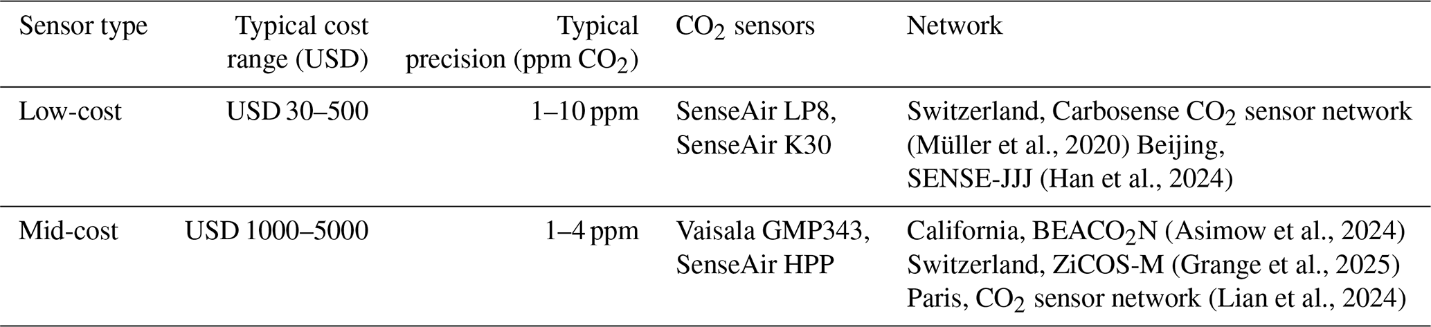
Recent advancements in medium-precision carbon monitoring technologies have enabled the establishment of high-density sensor networks with low to mid cost and medium precision, presenting a viable and competitive monitoring strategy (Müller et al., 2020; Shusterman et al., 2018). This approach effectively addresses the challenges posed by CO₂ variability in urban environments, where complex emission sources, vegetative carbon sinks, and dynamic meteorological conditions interact. Unlike high-precision instruments (0.1 ppm) such as Picarro cavity ring-down spectroscopy (CRDS) analyzers (Picarro, 2023), which cost approximately USD 100 000; low-cost (USD 30–500); and mid-cost (USD 1000–5000) sensors utilizing non-dispersive infrared (NDIR) technology (Table 1) (Han et al., 2025), offer a 1–10 ppm accuracy at a fraction of the price (USD 30–5000) – representing a cost reduction of more than an order of magnitude. This enhanced affordability facilitates large-scale deployment, making these sensors particularly attractive for comprehensive urban CO₂ monitoring systems (Lopez-Coto et al., 2017; Turner et al., 2016; Wu et al., 2016; Zeng et al., 2021).

While cost-effective, NDIR sensors are sensitive to environmental changes and often exhibit long-term drifts and abrupt jumps. Noise, environmental sensitivity, and temporal drifts result in raw measurements that typically have more significant errors and uncertainties than the accuracy and resolution required for urban CO₂ monitoring. The accuracy of these sensors typically depends on correction methods that account for environmental factors such as temperature, humidity, and pressure. However, the sensitivities of these variables can vary significantly, presenting major challenges in calibrating large sensor networks (Bigi et al., 2018; Delaria et al., 2021; Hagan et al., 2018; Martin et al., 2017). With careful correction – using environmental chambers and co-located high-precision instruments – these sensors can achieve short-term measurement accuracy within ± 1–3 ppm under controlled laboratory conditions (Cai et al., 2024; Grange et al., 2025; Müller et al., 2020).

Additionally, unlike high-precision instruments, NDIR sensors are more prone to temporal drift and fluctuations. To mitigate these issues, sensors are periodically re-calibrated at the laboratory or undergo in situ field calibration using traceable standard gases. While essential, these correction processes are labor-intensive and time-consuming. Some networks adopt alternative approaches. For instance, sensor-specific drift slope can be predetermined before deployment, with offsets corrected using the lower percentile (5 %–10 %) of observations across the entire network (Shusterman et al., 2016). Delaria et al. (2021) demonstrated that using the median value from at least 12 sites with minimal temperature dependence as a reference can maintain network precision at 3.6 ppm. Another method involves determining drift by comparing nearby instruments under specific weather conditions when horizontal CO₂ gradients are small (Müller et al., 2020). A widely used and robust calibration method involves automatic or manual standard gas injections. In the Beijing and Jinan networks, we applied this method across more than 160 instruments, with automatic standard gas calibration performed weekly. Results showed mean biases of −1.28 to −0.64 ppm at a 1-month scale (Cai et al., 2024). Manual standard gas calibration is particularly useful in mobile observations, such as on-road vehicle measurements and vertical profile observations using tethered balloons (Liu et al., 2021; Bao et al., 2020). However, calibration costs can be significant. For automatic standard gas calibration (weekly frequency), expenses reach approximately USD 300 per station per year, consuming two 8 L, 10 MPa gas tanks (one as a working standard and the other for quality control). Consequently, maintaining 100 stations with such low-cost sensors would incur an annual cost of USD 30 000 for standard gas alone.

Currently, several locations, such as California, Paris, Switzerland, and Beijing, have established high-density CO₂ monitoring networks utilizing NDIR sensors (Table 1). For instance, the Berkeley Environmental Air-quality and CO₂ Network (BEACO₂N) in California, USA, utilizes the Vaisala CarboCap GMP343 sensor (mid-cost), with a raw accuracy of ± 3 ppm +1 % reading (Vaisala, 2020). After correcting for bias and temporal drift using the in situ method, the observation accuracy is approximately 1–4 ppm (Shusterman et al., 2016, 2018), while the reported accuracy improved to 1.6–3.6 ppm after temperature correction (Delaria et al., 2021). The Carbosense CO₂ sensor network in Switzerland (Müller et al., 2020), which uses the SenseAir LP8 sensor (low-cost), with a raw accuracy of ± 50 ppm (SenseAir, 2019), achieves an observation accuracy of 8–12 ppm through initial laboratory chamber correction and regular drift calibration via ambient co-location with nearby reference instruments.

China aims at peaking carbon emissions before 2030 and achieving carbon neutrality before 2060 (the Dual Carbon Goals, DCGs) (He et al., 2020; Huang et al., 2023; Zeng et al., 2022). To support China's DCGs and address the high spatial variability in CO₂ concentration in urban areas, the Institute of Atmospheric Physics, Chinese Academy of Sciences (IAP), has established a network of 134 sites using SenseAir K30 sensor since 2017 (Han et al., 2024). This study presents the correction methods developed for the SenseAir K30 sensors and evaluates the accuracy achievable through the environmental dependence correction method based on laboratory simulation. At a field observation site in Beijing, environmentally corrected low-cost sensors (LCSs) were co-located with high-precision Picarro instruments for up to 30 months. By comparing the data with measurements from Picarro instruments, we gained more profound insights into the long-term performance and long-term drift characteristics of the LCS, as well as assessed the effectiveness of our long-term drift correction method. Our findings demonstrate that timely long-term drift correction significantly improved the accuracy of urban CO₂ monitoring networks based on LCS and reduced time, labor, and money investment. This research provides valuable evidence for optimizing the deployment and maintenance of LCS-based monitoring networks in urban environments.

2 The application of SenseAir K30 sensors for urban CO₂ monitoring

A multivariate linear regression analysis was used for environmental correction, which can improve the accuracy of the SenseAir K30 sensor from its initial specification of ± 30 ppm ± 3 % of reading (SenseAir: K30 products sheets, 2022) to a range of 1.7–4.3 ppm (Martin et al., 2017). The environmentally corrected K30 sensor demonstrated reliability and consistency when compared to higher-precision instruments and standard gas under a controlled indoor environment with a root mean square error (RMSE) ranging from 1 to 3 ppm on a monthly scale (Cai et al., 2024). Furthermore, the low-cost sensor exhibited highly consistent with Picarro system during on-road observations conducted using the same vehicle with an RMSE of 3.6 ppm (Liu et al., 2021). In a study by Bao et al. (2020), the sensor was utilized to measure the CO₂ vertical profile in the lower troposphere in Hebei Province, China, showing good consistency with traditional gas chromatography measurements (Bao et al., 2020). Additionally, Cai et al. (2024) applied the low-cost sensor in an industrial park, revealing a CO₂ concentration enhancement of 5–28 ppm within the park compared to a reference site (Cai et al., 2025a).

The Beijing–Tianjin–Hebei (or Jing–Jin–Ji, JJJ) network, deployed with low-cost sensors, has provided valuable insights into seasonal variations, urban–rural differences, and the homology of CO₂ and PM_2.5 (Han et al., 2024). The low-cost sensors have also been proven effective in detecting signals related to COVID-19. Continued CO₂ measurements in Beijing showed a 15 ppm reduction during the 2020 lockdown period compared to the before and after periods. Similarly, regular on-road CO₂ observation in Beijing before, during, and after COVID-19 lockdown showed a 40–60 ppm decrease during COVID-19 lockdown period (Liu et al., 2021). These applications demonstrate the versatility and reliability of low-cost sensors in capturing both environmental and anthropogenic influences on atmospheric CO₂ concentrations.

3 Instrument design and correction methods of SENSE-IAP

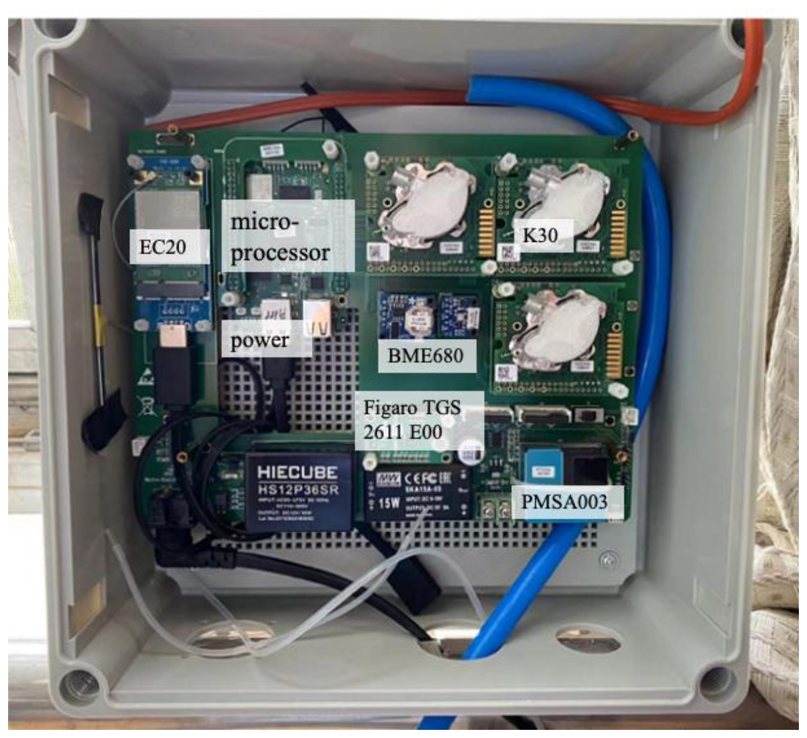
The SENSE-IAP instrument integrates three K30 sensors alongside a Bosch BME680 (BME) sensor (Bao et al., 2020; Liu et al., 2021), all collected by an updated version of BeagleBone Green Wireless (BBGW). The standard version of SENSE-IAP instrument also includes a Figaro TGS 2611 sensor for CH4 detection and a Plantower PMSA003 for PM_2.5 measurements. These components are compactly integrated onto a single circuit board and housed within a weatherproof enclosure, as illustrated in Fig. 1.

The BME sensor is positioned close to the K30s to simultaneously monitor the temperature (T in °), relative humidity (RH in %), and pressure (P in hPa) of the air mass inside the instrument. This design ensures real-time correction of the sensor response values, accounting for dynamically changing external environmental conditions and enhancing measurement accuracy.

Figure 1 The layout of sensors in the standard version of SENSE-IAP instrument.

To improve the observing accuracy, we developed a CO₂ calibration system incorporating both controlled environmental experiments and calibration software (Bao et al., 2020; Han et al., 2024; Liu et al., 2021). The system follows these main steps: (1) converting raw electrical signals to CO₂ values within atmospheric observation ranges; (2) resampling data from 2 s to 1 min to reduce white noise; (3) applying environmental corrections of temperature, humidity, and air pressure during span calibration; and (4) performing calibration using standard gas traceable to the WMO X2007 scale (identical to the standard used in high-precision systems like Picarro instruments) to remove system bias. The controlled environmental experiments typically require 1 week of co-location with a reference instrument to determine environmental correction coefficients followed by another week of co-location for post-quality check. To fully characterize long-term drift patterns, we recommended maintaining observations for at least 1 year to capture seasonal variations (including both summer and winter cycles).

The raw signals from all sensors were collected at a frequency of 2 s with a standard deviation of approximately ± 4 ppm. Figure 2 shows the experimental results of continuously introducing standard gas over 25 h to evaluate the instrument's noise characteristics. As shown in Fig. 2, the Allan deviation (in ppm) decreases with increasing integration time. At a 2 s measurement interval, the noise level is 4 ppm, which decreases to approximately 0.2 ppm for integration times ranging from 2 min to 1 h. However, the Allan deviation increases after 1 h of integration time, indicating the presence of drift contributions.

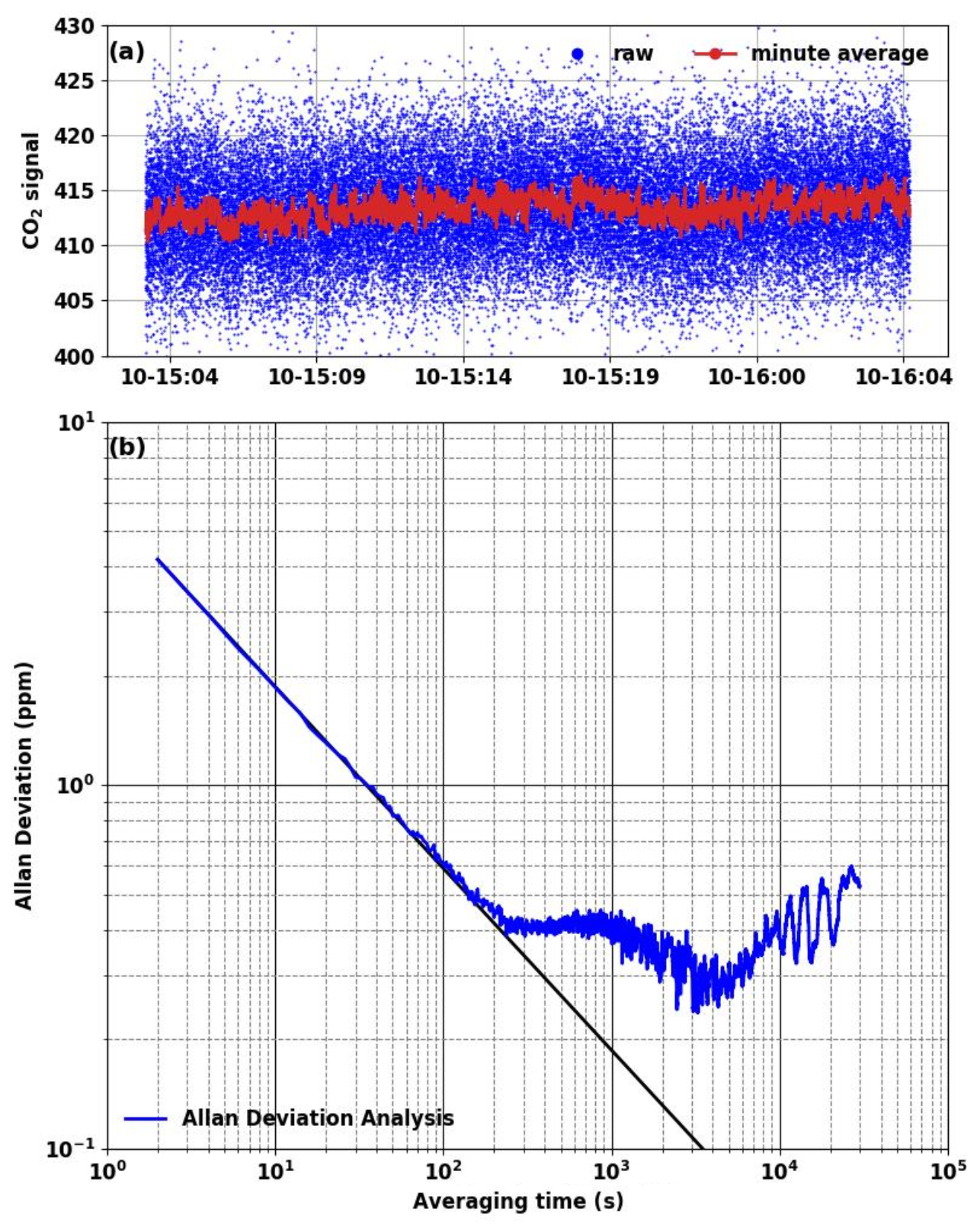
Figure 2 (a) The raw signals measured continuously over 25 h from 03:00 UTC on 15 October to 03:00 UTC on 16 October 2022. (b) Allan deviation log plots.

In addition to white noise, the raw signals often contain outliers that must be removed through quality control. According to Eq. (1), following the 3σ principle, the original data points x_i collected during the sampling period are treated as samples. The average value $\stackrel{\mathrm{‾}}{x}$ of non-missing x_i is calculated, and the standard deviation (SD) of the x_i is σ. If $|x_i-\stackrel{\mathrm{‾}}{x}|>\mathrm{4}\mathit{\sigma }$, the data point is identified as an outlier and removed. We adopted the 4σ threshold to strike a balance between effectively removing outliers and preserving the natural ranges of variability in the data.

$$\begin{array}{}\text{(1)}& \mathit{\sigma }=\sqrt{{\displaystyle \frac{{\sum }_{i=\mathrm{1}}^n{\left(x_i-\stackrel{\mathrm{‾}}{x}\right)}^{\mathrm{2}}}{n-\mathrm{1}}}}\end{array}$$

Subsequently, the raw signals are averaged from a 2 s interval to a 1 min interval (resample) to reduce standard deviation. A 1 min integration time was chosen as an optimal trade-off between noise reduction and maintaining sufficient time resolution to track natural variations in CO₂ concentrations accurately. As in Eq. (2), the resampled value Y_i for each minute is calculated as the average of all non-outlier values x_j within that minute.

$$\begin{array}{}\text{(2)}& Y_i={\displaystyle \frac{{\sum }_{j=\mathrm{1}}^m{x}_j}{m}}\end{array}$$

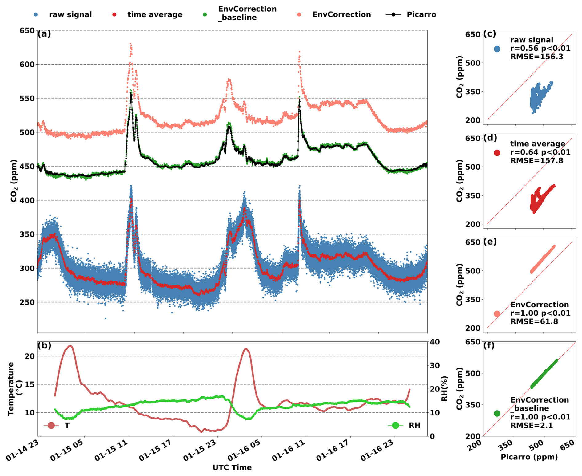
Figure 3 (a) Compared CO₂ at each processing step. (b) Synchronized monitoring of T and RH. (c–f) The scatter plots of CO₂ measurements form LCS and Picarro instrument at different processing steps, including (c) the raw signal in 2 s resolution, (d) the values after noise reduction at a 1 min resolution, (e) the CO₂ concentrations after environment corrections, and (f) systematic bias correction.

The correction system we developed substantially improves the accuracy of CO₂ measurements through a comprehensive process that includes outlier removal and noise reduction. Figure 3 shows the main steps of the correction system, with the data cleaning method described earlier constituting the initial two steps. As shown in Fig. 3a, the raw signal (blue) undergoes de-specking and denoising (red). However, a noticeable deviation remains between the LCS measurements and the true value, with a correlation coefficient (r value) of approximately 0.6 (Fig. 3c–d). The differences mainly come from environmental sensitivity and baseline deviations in concentration.

Similarly to the correction standards used in high-precision systems, our LCS units are calibrated using standard gas traceable to the WMO X2007 scale. This calibration adjusts the span and calibrates system bias before deployment. For the typical CO₂ concentration range (400–700 ppm), a concentration-dependent offset (ΔC) exists between the time-averaged LCS measurements and the standard gas concentration. Since this concentration dependence varies for each K30 sensor, laboratory corrections are essential for accuracy improvement. Our concentration correction process includes multiple concentration gradients, ensuring applicability to real-world monitoring scenarios. The fitting parameters of ΔC against the measured values are determined through regression analysis, enabling precise correction across the operational range.

$$\begin{array}{}\text{(3)}& \mathrm{\Delta }C=Y_{\mathrm{m}}-y_{\mathrm{0}},\end{array}$$

where y₀ represents the concentration of standard gas or the high-precision reference instrument (Picarro G2301); Y_m is the minute-averaged values from LCSs.

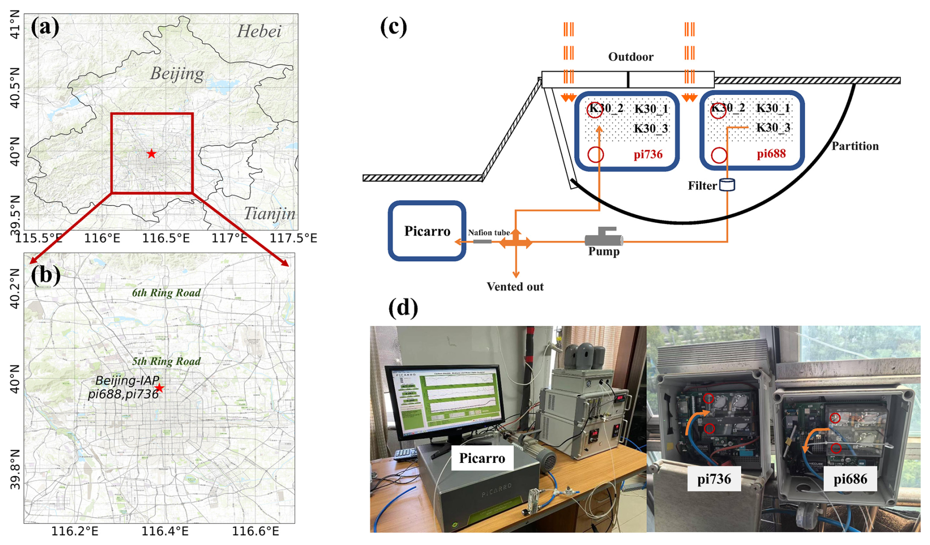
Figure 4 (a) Map of the location of Beijing-IAP in Beijing. (b) Map showing the location of Beijing-IAP within Beijing's main urban area. (c) The diagram of gas flow design for the synchronous observation system. (d) The photographs of the instrument installation setup. The source for the basemap used in panels (a)–(b) is ESRI (https://server.arcgisonline.com/arcgis/rest/services/World_Topo_Map/MapServer, last access: 16 June 2025).

Environmental calibration was conducted in an environmental controlled chamber. The LCS environmental sensitivity corrections included T compensation (10–50 °C in five steps), RH compensation (10 %–90 % in nine steps), and P compensation. This correction is based on sensitivity testing conducted in the laboratory (Martin et al., 2017), with comparisons made against Picarro. Each sensor is assigned unique sensitivity parameters through multivariate regression and iteration analysis.

$$\begin{array}{}\text{(4)}& \begin{array}{rl}\mathrm{\Delta }C& =f\left(a_T,Y_T\right)+f\left(a_H,Y_H\right)+f\left(a_P,Y_P\right)\\ & +f\left(a_C,Y_C\right)+\mathit{\epsilon },\end{array}\end{array}$$

where the baseline correction coefficient is ε; Y_T, Y_H, Y_P, and Y_C represent the compensation values for the T, RH, P, and concentration sensitivity, respectively, applied to the minute-averaged CO₂ measurement; a_T, a_H, and a_P are the regression coefficients against T, RH, and P, respectively; and a_C is the span correction coefficient against concentration.

Thus, the corrected CO₂ can be expressed as

$$\begin{array}{}\text{(5)}& \begin{array}{rl}C& =Y_m-(f\left(a_T,Y_T\right)+f\left(a_P,Y_P\right)+f\left(a_H,Y_H\right)\\ & +f\left(a_C,Y_C\right)+\mathit{\epsilon }).\end{array}\end{array}$$

The r values between the CO₂ corrected in the final two steps and the Picarro measurements are close to 1 (Fig. 3e–f). Additionally, the difference between the environmental correction (pink) and baseline calibration (green) in Fig. 3a represents the coefficient ε. After applying these correction steps, the accuracy of the LCS measurements improved to 1–4 ppm compared to Picarro (Liu et al., 2021).

Before deployment, the span and system bias of the LCSs were calibrated. However, once deployed to field stations, LCSs tended to drift on a weekly to monthly scale, necessitating time-dependent drift calibration. We defined S_cor as the starting time of drift and E_cor as the time when the drift slope stabilized or when calibration was required, with $\mathrm{\Delta }=E_{\mathrm{cor}}-S_{\mathrm{cor}}$. ΔC_drift represents the bias between the concentration C measured by the instrument and the standard concentration C₀ at E_cor. Using the Eq. (6), the drift rate over time (ppm min⁻¹) at E_cor is calculated (s_t). The b_cal is a constant deviation, representing the difference between the baseline and the standard value before long-term drift occurs (at S_cor). This value is generally considered to be zero since system bias has been calibrated before departure. The error at any time between S_cor toE_cor can be calibrated to $C_{\mathrm{Cor}}^{\mathrm{drift}}$ using the following formulas:

$$\begin{array}{}\text{(6)}& {\displaystyle }\mathrm{\Delta }{C}_{\mathrm{drift}}=s_t\mathrm{\Delta }t+b_{\mathrm{cal}},\text{(7)}& {\displaystyle }{C}_{\mathrm{Cor}}^{\mathrm{drift}}=C-\mathrm{\Delta }{C}_{\mathrm{drift}}.\end{array}$$

This integrated instrument with environmental correction and drift correction is named SENSE-IAP.

4 Co-located observation system

Our experiment has been conducted since July 2022 at IAP (Beijing-IAP site, Fig. 4a and b). Located in a central urban area with high population density, the Beijing-IAP site is significantly influenced by traffic emissions.

To evaluate the performance of the LCS, we developed a synchronous observation system that compares the LCS with high-precision instruments. This system includes two SENSE-IAP units (numbered pi688 and pi736), each equipped with three K30 sensors. A cavity ring-down spectrometer (Picarro G2301) was used as the high-precision instrument for CO₂ measurements (Picarro, 2023). The precision and accuracy of the Picarro instrument are better than 0.1 ppm (Yang et al., 2021). At Beijing-IAP, the Picarro analyzer was calibrated monthly using high-pressure standard gases provided by the Meteorological Observation Center of the China Meteorological Administration (MOC/CMA), which are traceable to the World Meteorological Organization (WMO) X2007 scale.

To ensure long-term synchronous observation between the LCSs and Picarro, deployment enables two sets of instruments to measure the same gas mass. This ensures that any differences in observed values only come from the effects of T, RH, and P, as well as the concentration span, all of which can be adjusted through correction methods. The deployment setup is shown in Fig. 4b–c.

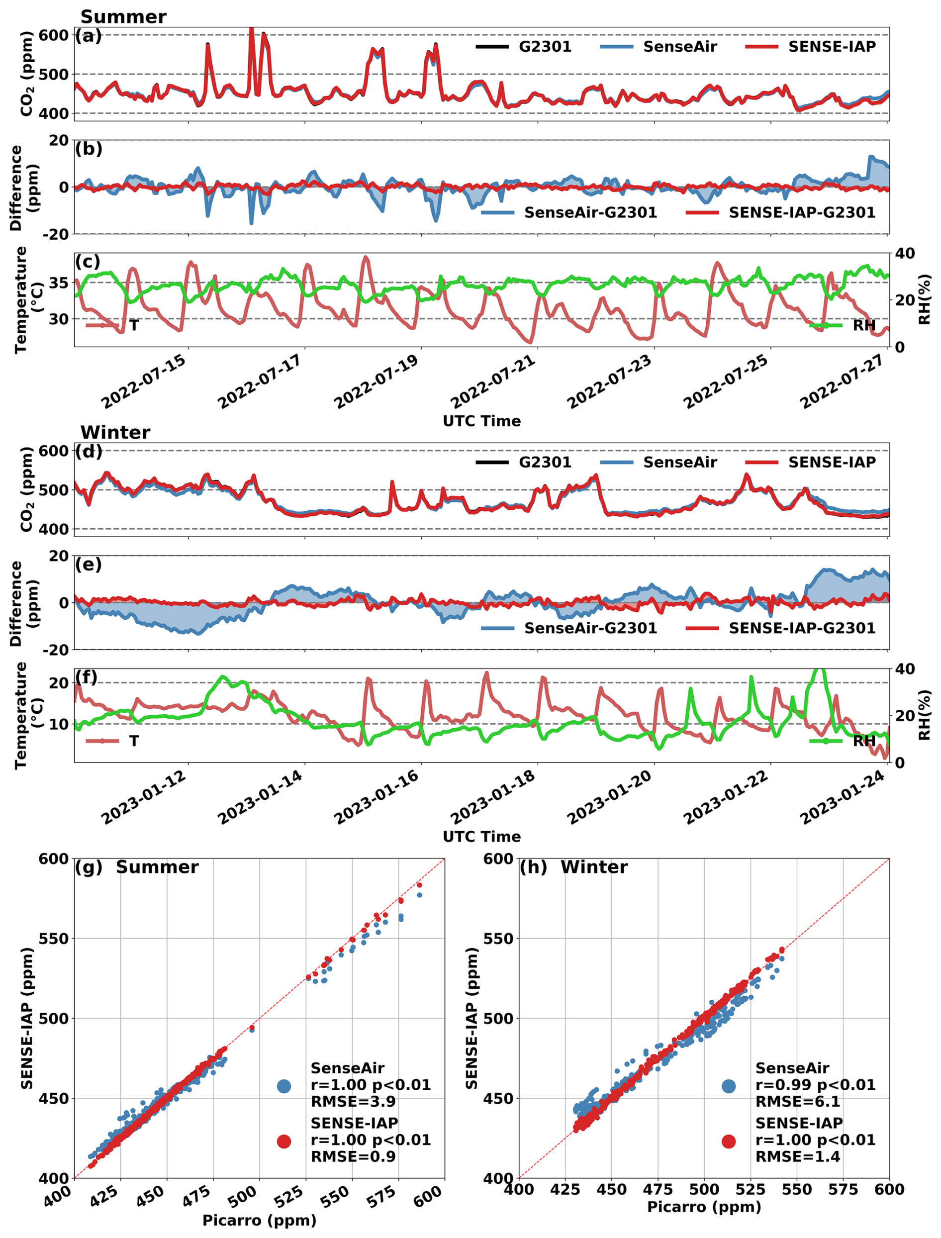
Figure 5 Comparison between hourly CO₂ concentrations measured by the SENSE-IAP and Picarro systems at the Beijing site from 13 to 27 July 2022 (a–c, g) and 10 to 24 January 2023 (d–f, h). We compared both the raw CO₂ data from SenseAir (blue) and the environmentally corrected data from SENSE-IAP (red) with that from Picarro (black). The T and RH were measured for the environment inside the instrument.

The instruments were mounted on the edge of an open window to directly measure the outdoor air and environmental changes, which were almost the same as field-deployed conditions (Figs. 4 and S8 in the Supplement). Temperature primarily ranged from 0–40° and RH typically between 0 % and 60 %. A partition isolated the LCSs from indoor spaces, ensuring measurements primarily reflected outdoor environmental conditions. Three K30 sensors and one BME sensor were housed in a transparent cover featuring two 2 mm diameter ventilation holes in the upper-left and lower-left corners (red circles in Fig. 4c and d). Air passively diffuses into the pi688 enclosure, while a 4 mm diameter blue tube connected to the cover's left side enabled active air sampling via an air pump (GAST DOA-P504-BN). Upstream of the pump, the airflow passed through a capsule-type 10 µm filter (COBETTER 92WM-LPF1000) for particulate matter removal (Fig. 4c). Downstream of the pump, a Nafion drying tube is installed for Picarro analysis (bypassed for SENSE-IAP measurements) (Fig. 4c). The filtered air is then divided by a four-way valve, delivering 3–5 L min⁻¹ to the pi736 and 0.3–0.4 L min⁻¹ to the Picarro analyzer, with excess air vented through the final outlet.

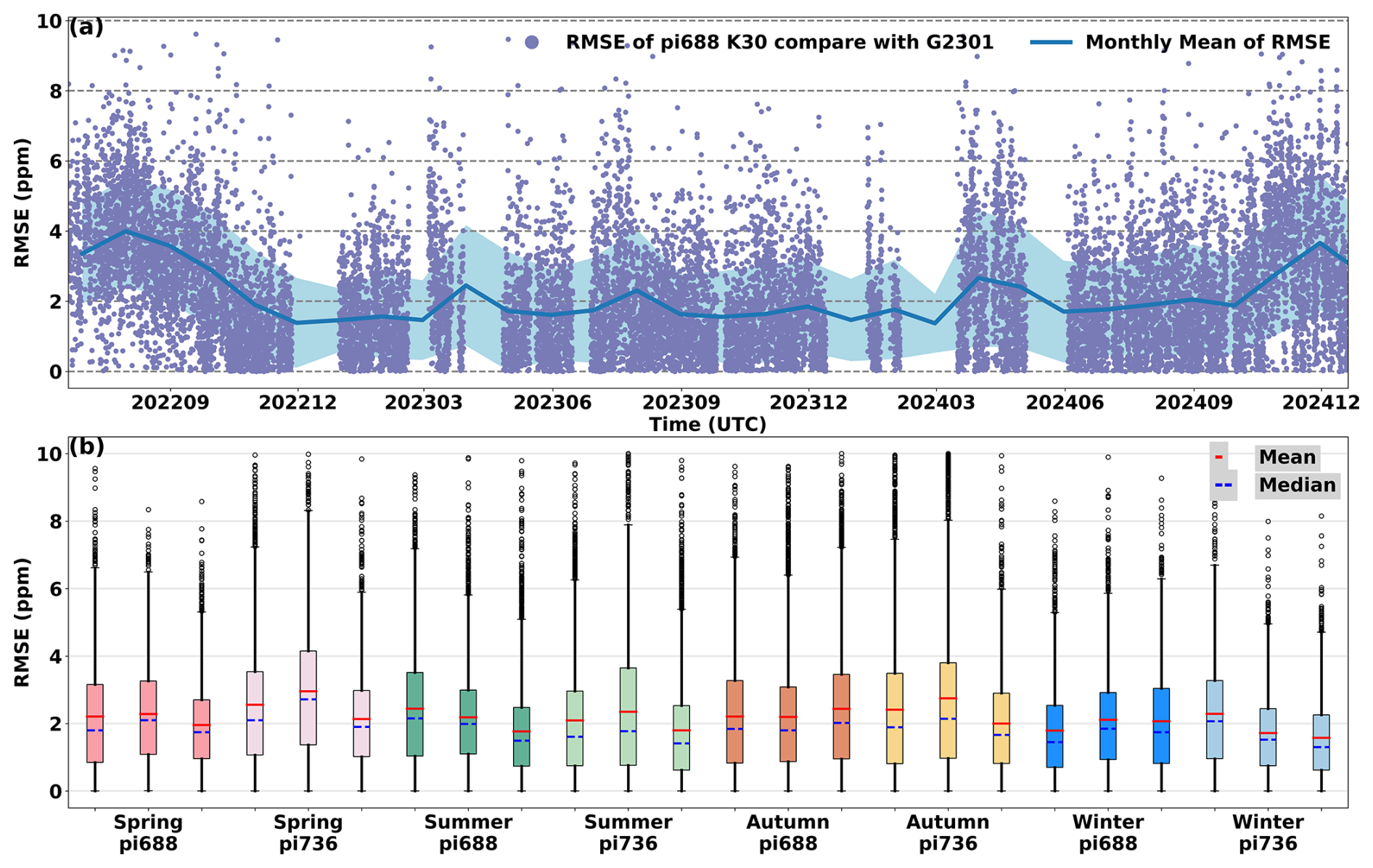
Figure 6 (a) The time series of daily RMSEs for hourly CO₂ concentration relative to Picarro (purple points) from June 2022 to December 2024, with a monthly rolling mean (blue line and shadow). (b) Box plot of the daily RMSEs of all six sensors across different seasons. Sensors from the same instrument are represented in the same colors (spring: dark pink/pink, summer: dark green/green, autumn: orange/yellow, and winter: dark blue/blue). Within each box, the red line indicates the mean value, while the blue dashed line represents the median values.

5 Environmental corrections for field measurements

To distinguish between the effects of short-term environmental factors and long-term drifts, we present these corrections separately. To focus specifically on the environmental corrections, all results in this section were obtained after removing long-term drift. A comprehensive discussion of long-term drift is provided in Sect. 5. Figure 5 shows the results from environment-corrected SENSE-IAP at the Beijing- IAP site compared with those from the Picarro system. After approximately 2 weeks of data collection during both summer and winter, the SENSE-IAP showed highly consistent results with Picarro, with RMSEs of 1.6 ppm in summer and 1.8 ppm in winter. In contrast, the raw CO₂ concentration data from the SenseAir showed a higher RMSE of 6.2 ppm in summer and 7.0 ppm in winter. Furthermore, the effectiveness of environmental correction is evident across different seasons.

The correction system effectively adjusted the CO₂ concentration within the 400–700 ppm measurement range. As shown in Fig. 5b, during the period from 16 to 19 July, even when the ambient CO₂ concentration experienced significant fluctuations, the instrument showed high consistency with Picarro. The T and RH detected by the BME sensor were used to monitor the instrument's internal environment. Notably, in winter mornings, sunrise caused a significant temperature increase due to the presence of metal components on the circuit board (Fig. 5f). Our environmental correction successfully corrected for the temperature dependence, as the deviation between the SenseAir and Picarro showed a strongly correlated with temperature in both seasons (Fig. S1a). Additionally, the deviation of SenseAir relative to Picarro was significantly associated with RH in summer (Fig. S1b), and our correction system incorporated humidity, which was related to ambient temperature. Compared to the raw SenseAir data, the consistency of all six sensors improved markedly, with the RMSE decreasing from 5.0 ± 1.0 to 1.3 ± 0.2 ppm in summer and from 6.8 ± 0.8 to 2.0 ± 0.4 ppm in winter (Fig. S2).

Table 2 The long-term drift trend of six sensors (unit: ppm per month).

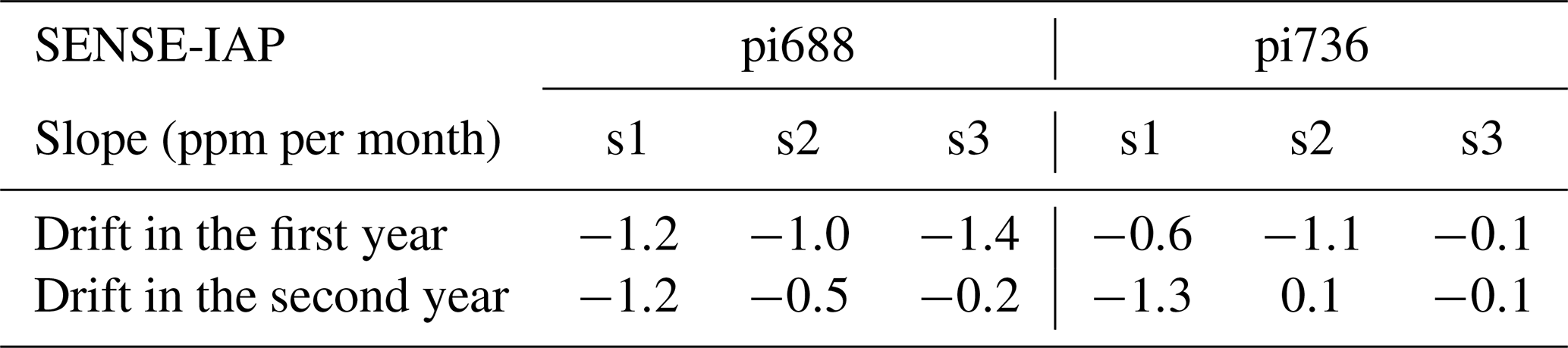
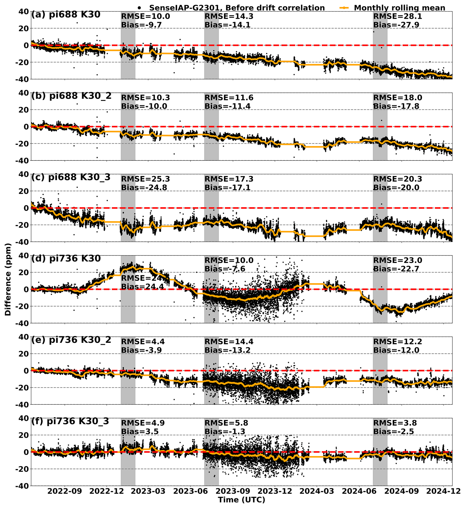
Figure 7 Time series of ΔCO₂ for the six sensors at the Beijing-IAP from June 2022 to December 2024 (black), with the monthly rolling mean (yellow line). The gray shadow represents the 1-month time range used to evaluate the RMSE and bias for each sensor after half a year, 1 year, and 2 years of deployment.

Our correction system can perform environmental sensitivity analysis and correction on individual sensors, with the correction efficacy remaining robust across seasonal environmental changes. We further analyzed the daily RMSE of the SENSE-IAP relative to Picarro during 30 months of co-located observation. As shown in Fig. 6a, the daily RMSE of one sensor (pi688-K30) ranged from 1.5 to 4.0 ppm throughout the observation period, with the light blue shadow representing the monthly mean ± standard deviation. The average and median of daily RMSEs for this sensor were less than 2.0 ppm (Fig. 6b), except for an increase to higher than 2 ppm in summer (dark green). Compared to Picarro, the consistency of SENSE-IAP was better in winter, with an RMSE below 2.0 ppm on most days. Except for a few sensors exhibiting slightly higher RMSEs (approximately 3.0 ppm) in spring and autumn (pi732-K30), the daily RMSEs of the six sensors showed no significant seasonal variation (Fig. 6b).

6 Performance of typical long-term drift and correction method

After environmental correction, the six SENSE-IAP sensors were co-located with a Picarro analyzer synchronously for over 30 months. As shown in Fig. 7, two types of long-term drift were identified: (1) a downward drift trend and (2) a seasonal drift cycle. While the environmental correction system effectively corrects the impact of diurnal environmental changes (Fig. 6), significant errors occurred in sensors due to the two types of long-term drift. Without the long-term drift calibration algorithm, the bias of SENSE-IAP could reach 27.9 ppm with an RMSE of approximately 28.1 ppm (Fig. 7).

Table 3 Evaluation parameters^* of the CO₂ concentration measured by K30 sensors compared to those from Picarro, including SenseAir-Corrected values, Raw signal, and SENSE-IAP at the Beijing-IAP from June 2022 to December 2024 (unit: ppm).

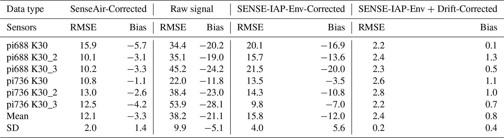
^* According to the statistical results of 24 h running means.

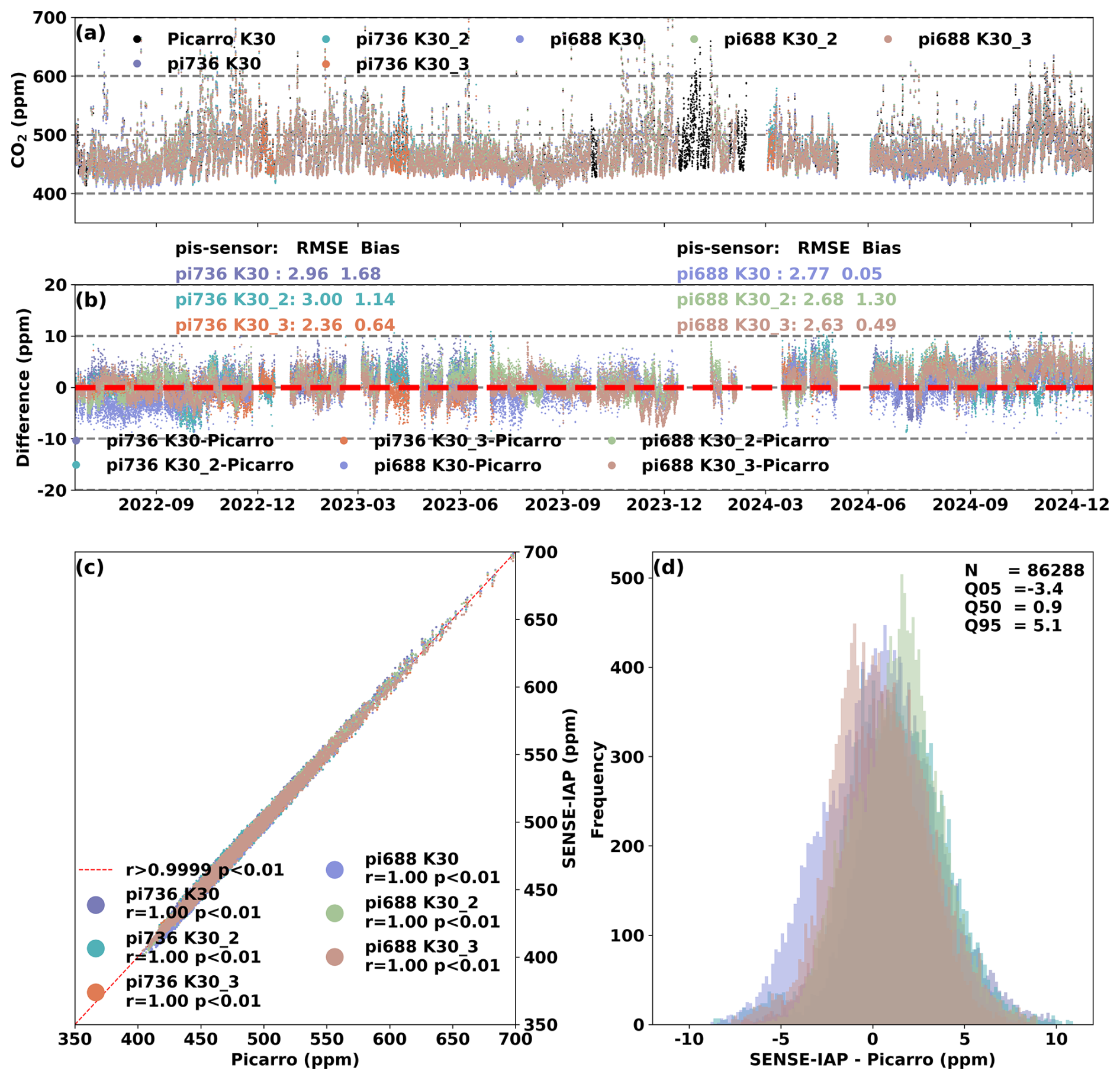
Figure 8 (a) Comparison of hourly CO₂ concentrations measured by six sensors and Picarro at Beijing-IAP from June 2022 to December 2024. (b) The time series of ΔCO₂. (c) Scatter plot of SENSE-IAP and Picarro. (d) Histogram plot of the ΔCO₂.

During the observation period, all six sensors exhibited long-term downward drifts ranging from 0.1 to 1.2 ppm per month (Fig. 7 and Table 2). Among the six sensors deployed in this study, only pi736 K30_3 showed a drift trend of less than 0.1 ppm per month (Table 2). For sensors such as pi688-K30 and pi688-K30_2, the ΔCO₂ displayed a continuous downward trend over the 30 months, with slopes of 1.2 and 1.0 ppm per month, respectively (Table 2). Notably, the drift trends for these sensors did not show significant stabilization over time.

In addition to the downward drift trend, sensors like pi688-K30_3 and pi736-K30 exhibited varying seasonal cycle trends. After 6 months of deployment, these sensors showed RMSEs of 25.3 and 24.8, respectively (Fig. 7). However, after more than 1 year of observation, the impact of seasonal drift decreased, and the errors caused by long-term drift were highlighted, resulting in reduced RMSEs as 17.3 and 10 ppm, respectively. The RMSE evaluation was conducted during the identical period employed for drift correction.

From the perspective of drift magnitude, a significant bias of 5 ppm (approximately 1 % of the ambient CO₂ concentration) typically occurred within 3–10 months after calibration, with most cases observed within 5 months. The seasonal drift cycle occurred on a 6-month scale, with maximum errors typically occurring in winter and summer. Therefore, we recommend that the long-term drift calibration frequency of SENSE-IAP should be no less than 3 months and no longer than 6 months. In addition, drift calibration should be performed at least once during both winter and summer seasons. If the target monitoring accuracy is within 3 ppm, the drift calibration frequency should be at least every 2 months, as a 3 ppm bias typically develops within 2–5 months.

The method for the long-term drift calibration is as follows. According to functions 6–7, we illustrate our long-term drift calibration method by focusing on the first year of observations. At the start of the observation period (June 2022), we adjusted the baseline of the six sensors. We designated the initial calibration time point as S_cor for the first observation period (June 2022 to January 2023). The inflection point of the drift trend in February 2023 was identified as E_cor for the first period and as S_cor for the second period of the observation (January to September 2023). The E_cor for the second period was set to September 2023 in this study. We applied the linear calibration method between these two time points for both periods of the drift trend. After calibration, the CO₂ concentrations from the six sensors showed strong consistency with the Picarro, with an RMSE ranging from 2.4–3.0 ppm (Fig. 8).

It should be noted that due to the loose connection of ventilation pipeline between July 2023 and March 2024, the CO₂ concentration measured by pi736 and Picarro were not strictly synchronized. This issue led to a relatively lower short-term monitoring accuracy during this period, primarily due to the lag effect caused by air diffusion. To assess the actual hourly monitoring accuracy of SENSE-IAP, we excluded data from this period. Without this exclusion, the RMSE for pi736 would have been 3.9–4.5 ppm (Fig. S3). However, to ensure the completeness and robustness of the long-term drift analysis, we retained samples from this period, allowing for a more comprehensive evaluation of drift trends over time.

7 Comparison of data quality across multiple levels over a long-term scale

As previously mentioned, the correction system effectively corrected the sensors' short-term environmental dependence. By applying a linear calibration method at least every 3 months, we can calibrate the time-dependent drift of LCSs and resolve residual seasonal cycles that the environmental correction system cannot fully resolve. This seasonal variation is prominently reflected in the original electrical signal (raw signal). As shown in Fig. S4b, we eliminated the influence of short-term environment changes through a 24 h running mean, revealing that the seasonal drift cycle in the raw signal can reach up to 100 ppm with an RMSE of 38.2 and a bias of −21.1 ppm (Table 3).

The defining characteristic of medium-precision low-cost sensors is the presence of long-term drift. This drift, which exhibits a downward trend, is observed in all sensors, with variations only in the drift rate (Fig S5). Long-term drifts resulted in an RMSE of 15.8 and a bias of −12.0 for the LCS, respectively (Table 3). Although seasonal cycle does not significantly alter the overall trend of long-term drift, seasonal environmental variations can introduce errors of up to 25 ppm if baseline calibration are performed only annually (Fig. 7). Therefore, we recommend that baseline calibration be conducted at least every 6 months, ideally during both winter and summer.

The data provided by the SenseAir manufacturer were corrected for temperature sensitivity using the default temperature parameters. The long-term drift was calibrated using a so-called ABS algorithm, which employs periodic one-point calibration in SenseAir, assuming that the minimum value of CO₂ concentration is 400 ppm in fresh air (SenseAir-Corrected data). However, due to the constant assumption of fresh air concentration, coupled with the carbon absorption of vegetation in summer and the higher emissions in winter, the SenseAir-Corrected data exhibit a fluctuating trend of approximately 20 ppm, with higher values in summer and lower values in winter. Consequently, the bias of SenseAir-Corrected data can be −3.3 ± 1.4 ppm with an RMSE of 12.1 ± 2.0 ppm (Fig. S6, Table 3). In contrast, the drift-calibrated SENSE-IAP data demonstrate a much smaller bias (0.8 ± 0.4 ppm) and an 80 % improvement in accuracy with an RMSE of 2.4 ± 0.2 ppm (Fig S7, Table 3).

8 Seasonal drift cycle effects on SENSE-IAP

As shown in Fig. S8, the seasonal variations observed before instrument linear calibration were correlated with T, RH, and P. The ΔCO₂ between pi736-K30 and Picarro significantly correlated with all three environmental factors, with r values of −0.58, −0.46, and 0.33 against T, RH, and P, respectively. In contrast, the relationship between pi688-K30_3 and environmental factors was opposite to that of pi736-K30, with r values of 0.33, 0.5, and −0.6 against T, RH, and P, respectively. Considering seasonal phase differences between CO₂ concentration changes and environmental factors, this seasonal deviation was likely attributable to not only insufficient environmental compensation but also the influence of seasonal effects on the instrument's physical properties. For instance, changes in the sensor's optical cavity size caused by thermal expansion and cold contraction can change the optical path lengths, subsequently affecting the pressure within the optical cavity and the strength of infrared CO₂ absorption (Yao et al., 2023). However, this hypothesis cannot fully explain why the two sensors, pi688 K30_3 and pi736 K30, exhibited opposite drift directions during the same season.

Long-term drift is typically observed in low- and mid-cost NDIR CO₂ sensors. Although our findings provide valuable references data specifically for K30 sensors, the recommended calibration frequency and observed seasonal cycle characteristics may also apply to other similar NDIR sensors. The calibration method we employed is universally applicable and effective for long-term drift corrections. For other NDIR sensors, we recommend selecting several representative samples for co-location with a high-precision instrument under field conditions for a minimum of 1 year to fully characterize their performance. This extended co-location period is crucial for comprehensively for evaluating both long-term drifts trends and seasonal drift patterns. Such characterization studies provide essential guidance for implementing remote calibration in high-density sensors networks. Alternatively, standard gas calibration serves as a practical substitute method. Based on our experimental results, we recommend a calibration frequency of at least once every 1 to 3 months for this approach.

9 Conclusions

We evaluated low-cost NDIR CO₂ sensors using Picarro as a reference instrument. Our environmental correction system effectively corrected the impact of short-term daily environmental changes by assigning unique environmental sensitivity parameters to each sensor. This approach reduces the short-term RMSE from 5.9 ± 1.2 ppm for SenseAir to 1.6 ± 0.5 ppm for SENSE-IAP. The correction system demonstrates robustness against seasonal environmental variations, maintaining a daily RMSE of 1–3 ppm.

Based on a 30-month observation, we recommend that the calibration frequency for long-term drifts do not exceed 6 months. For optimal performance and to ensure the target monitoring accuracy remains within 1 % of the ambient CO₂ concentration, a 3-month calibration interval is recommended. If standard instruments, standard gases (which are generally easier to obtain) or other reliable concentration references such as model simulations are available, long-term drift can be linearly corrected at the seasonal scale.

Consequently, after deployment, even with significant environmental changes around the instrument, there is no need to frequently bring the instruments back to the laboratory for re-correction of environmental impacts. After the long-term drift calibration, the RMSE of SENSE-IAP remains 2.4 ± 0.2 ppm even after 30 months of operation. This performance enables long-term deployment of the instruments, significantly reducing the maintenance costs associated with LCS.