Urban pollution monitoring with the AOTF-based NO₂ camera: validation with other DOAS instruments

Elevated surface concentrations of nitrogen dioxide (NO₂) are associated with poor air quality, making its detection and monitoring important for human health and the environment. Existing instruments such as the TROPOMI satellite currently deliver daily global maps of NO₂ tropospheric columns, and the future Sentinel-4 instrument will return hourly maps. While areas of strong concentrations (cities, large industries) can be detected in these satellite observations, their spatiotemporal resolution remains too coarse to capture local hot spots and quick variations.

In the context of urban air quality monitoring, we present a new type of remote sensing instrument capable of observing spatial and temporal gradients in the NO₂ field, which is not currently possible with either space instruments or from the routine operations of conventional diffraction grating and other ground-based remote sensing instruments. This novel instrument is based on an acousto-optical tunable filter (AOTF) located at the heart of a telecentric imaging system. The instrument acquires spectral images in the region 430–455 nm, where NO₂ exhibits strong absorption features. A dense spectral sampling was commanded in order to enable the application of the DOAS (differential optical absorption spectroscopy) method in the processing of the spectra measured by each detector pixel.

In March 2024, the instrument was deployed at the BAQUNIN supersite for atmospheric research, located in the center of Rome. In order to validate the NO₂ camera measurements, coincident acquisitions by a MAX-DOAS and a Pandora spectrometer were performed. The results show very good agreement among the three instruments. They also illustrate the additional capabilities of the NO₂ camera in observing the spatial and temporal variability of the urban NO₂ field.

1 Introduction

Humans are directly exposed to the chemical composition of Earth's boundary layer, the lowest part of the troposphere where emissions from the surface are mixing. In that layer, the nitrogen oxides (NO_x) family is made of nitrogen oxide (NO) and nitrogen dioxide (NO₂), the former being primarily released in combustion processes (both natural or anthropogenic) and the latter being produced by reaction of NO with ozone (O₃) or hydroperoxy radical (HO₂). Through photolysis, NO₂ can be converted back into NO, such that a photochemical equilibrium persists most of the day. Among other effects, high levels of NO_x are associated with poor air quality, given the role of the molecule in the advent of photochemical smog episodes (Seinfeld and Pandis, 2006).

Of these NO_x compounds, nitrogen dioxide (NO₂) is the most important for human health (World Health Organization, 2021). There is scientific evidence that chronic exposure to NO₂ can cause emphysema (Last et al., 1994) and that, together with ozone, it increases oxidative stress in the small airways within the lungs (Morrow, 1984). Long-term exposure to ambient NO₂ is found to be correlated with increased mortality (Chen et al., 2024; Huangfu and Atkinson, 2020).

This negative influence on human health prompted the World Health Organization (WHO) to release Air Quality Guidelines, updated in 2021 and more recently translated into a European law (Directive 2022/0347). While European Union Member States are required to deploy air sampling stations, with some guidelines on the number of stations and their location, the Directive fails to address the problem of the large variation of exposure by citizens living in different neighborhoods of close proximity. Such large differences have been observed in citizen science projects, such as the CurieuzenAir/CurieuzeNeuzen experiment, in which thousands of sampling flasks were deployed in both Brussels (Lauriks et al., 2022) and Flanders (De Craemer et al., 2020). The WHO identifies this inadequate monitoring of spatial variations in the concentration of pollutants such as NO₂ as one of the main gaps in the global coverage of air pollution monitoring (World Health Organization, 2021). These spatial and temporal differences are especially pronounced in urban environments.

In recent years, several new remote sensing instruments have been developed that attempt to capture this variability of the NO₂ field with high spatial and temporal resolution. These instruments work in the UV-visible wavelength range, where NO₂ is a strong absorber. Many consisted in grating instruments, whose field of view is steered mechanically (Manago et al., 2018; Peters et al., 2019; Mettepenningen et al., 2024). Retaining all the strengths of the differential optical absorption spectroscopy (DOAS) technique (Platt and Stutz, 2008), the images are constructed slice by slice, which is subject to artifacts in the case of a dynamic scene. One prototype of a native NO₂ imaging instrument relied on the gas correlation technique (Kuhn et al., 2022) but was tested only on large point source plumes. Another concept studied the potential of a Fabry–Pérot interferometer-based polychromatic imaging system for atmospheric trace gases remote sensing, including NO₂, with an elaborated use of the periodic structures of the species cross-sections (Kuhn et al., 2019); to our knowledge, no real-world application of this concept to the measurement of NO₂ has yet been realized.

An acousto-optical tunable filter (AOTF)-based instrument produced high spatiotemporal maps of NO₂ in the plume released by a thermal power plant (Dekemper et al., 2016). While the concept requires sweeping over wavelengths, it is a native imaging system with relatively high spatial resolution compared to other techniques. This paper discusses the improvements made to this instrument and demonstrates its capability to make quantitative measurements of the NO₂ field.

2 The improved AOTF-based NO₂ camera

The AOTF-based NO₂ camera concept stems from the ALTIUS instrument, an ESA satellite mission for the monitoring of the stratospheric O₃ layer that relies on the acquisition of spectral images of the atmospheric limb at selected wavelengths (Fussen et al., 2019). As part of the ALTIUS mission pre-developments, a proof-of-concept optical breadboard of its VIS channel was produced and tested in the laboratory. Although not meant to leave the laboratory, its potential for imaging NO₂ plumes was recognized and tested during the AROMAT-II campaign (Merlaud et al., 2020). That version of the instrument and the results of the campaign were fully described in Dekemper et al. (2016).

The instrument reported here is an improved version of the original breadboard in almost every aspect, from basic parameters such as reduced size and mass to improved optical performance and acquisition software (see Sect. 2.1). Its raw data remain monochromatic images stacked in hypercubes. During the AROMAT campaign operations, only four wavelengths were acquired. In Rome, routine operations included wavelengths between 427 and 454.9 nm, sampled every 0.15 nm. Further details of the wavelength sampling are described later in Sect. 4. This allows applying a DOAS algorithm and achieving higher accuracy.

In Sect. 2.1, we describe the instrument, its operating scheme and the raw data it produces. Sections 2.2 and 2.3 discuss the spectral response function of the instrument and the data acquisition, respectively. Then, in Sect. 2.4, we discuss the main differences between this instrument and the conventional diffraction grating-based spectrometers that are currently used to monitor the field of NO₂ as part of operational networks.

2.1 Instrument description

The fundamental instrumental concept described in Dekemper et al. (2012) and Dekemper et al. (2016) has been kept: a telecentric front-end module captures the light and sends it on to the AOTF. Upon crossing the crystal, a narrow band of the incident light spectrum experiences a coupling with the acoustic beam created in the crystal by a piezo-electric transducer. The acousto-optic interaction diffracts the selected part of the spectrum into another direction, such that two beams leave the AOTF: one containing photons of the same energy (the monochromatic beam) and the other containing the rest of the spectrum (the white beam). The back-end optics captures only the diffracted beam, which forms the monochromatic image on the detector. The selection of another wavelength happens by tuning the acoustic wave frequency. Figure 1 shows a picture of the optomechanical system. The fundamental physics of acousto-optic interaction in birefringent crystals is described in Harris and Wallace (1969); Chang (1974). Further details on telecentric systems using AOTFs can be found in, e.g., Suhre et al. (2004), and a discussion on the optimization of AOTF parameters used for spectral imaging applications is provided in Voloshinov et al. (2007).

Figure 1 The current optics setup, made with commercial off-the-shelf components.

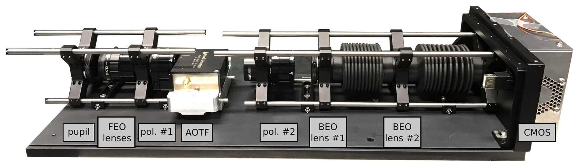
One of the most significant improvements concerns the field of view (FoV), which was increased to 23°×23° by reducing the focal length of the telecentric lens. The size of the back-end optics was also reduced by using shorter focal lengths. As a consequence, the instrument is now much more compact (see Table 1) and can be manipulated by a single person. The electronics (radio frequency (RF) generation and amplification, single-board computer) fit in a separate box. For the validation campaign, a pan-and-tilt head was used to control the pointing of the instrument (EKO sun tracker with a GPS receiver). The optics, electronics and pointing modules were all placed on a tripod. The camera housing was redesigned to withstand adverse weather; the optics were sealed off from the outside, while the cooled detector was partially outside this sealed environment, so that fresh air could reach the cooling block of the Peltier element. Figure 2 shows the exterior of the camera and its surrounding environment during the campaign.

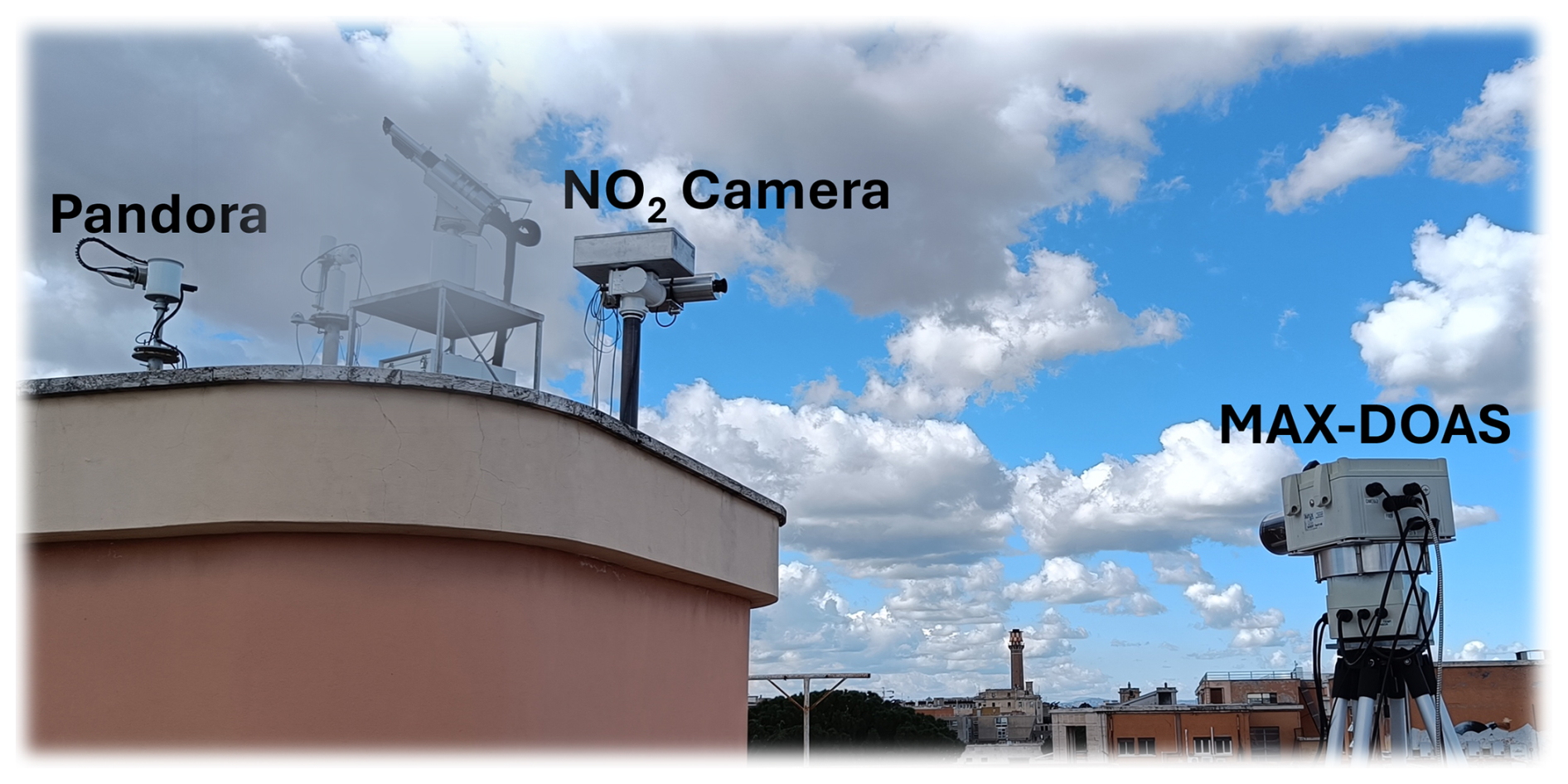
Figure 2 The NO₂ camera and the two reference instruments installed for the campaign at the BAQUNIN-APL supersite.

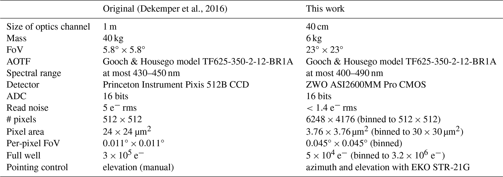
Table 1 details the specifications of the original versus the newer version of the NO₂ camera.

(Dekemper et al., 2016)

Table 1 Comparison of the original and current versions of the NO₂ camera.

The software reliability was tackled with newly designed control software that runs on an ARM-based single-board computer. An OKdo Rock 5B with 8GB RAM was selected for this purpose. It accepts an NVMe M.2 SSD to temporarily store the acquired images. It is responsible for the synchronized operation of the detector, RF electronics and EKO. At night, the raw measurement data are transferred automatically to storage servers over the internet.

2.2 Spectral response function

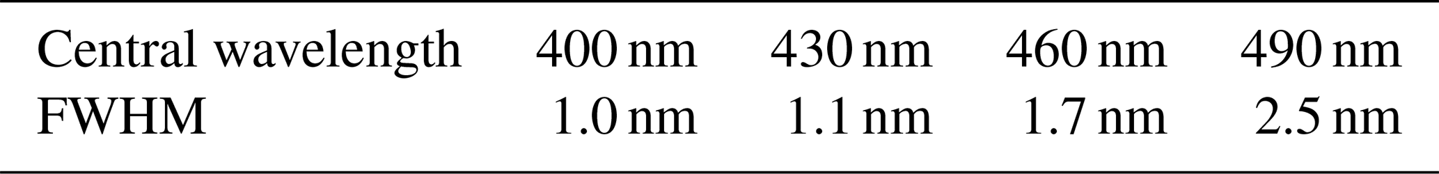
The instrument's spectral response function (SRF) is approximated by a variable-width Gaussian convolution scheme, where the full width at half maximum (FWHM) of the kernel evolves as a function of the central wavelength, as shown in Table 2. These choices were made from fitting the convolved theoretical solar spectrum (Chance and Kurucz, 2010) to the measured intensity at zenith during a calibration experiment. The merit function for the fit was the mean absolute difference between both spectra, after taking their logarithm and subtracting a low-order polynomial approximation from each.

Table 2 Instrument's spectral resolution (width of Gaussian kernel) as a function of the wavelength. A linear interpolation is performed between the values shown here.

2.3 Data acquisition

The image projected on the CMOS detector is roughly square. Of the full rectangular native resolution of 6248×4176 pixels, only a square region of interest of 4096 by 4096 pixels is selected. The resulting image is then binned in two steps. A first 4×4 binning is executed by the detector itself, then the software bins the image again, leading to a final resolution of 512 by 512 pixels. The main motivation for binning is the increase in the signal-to-noise ratio (SNR) by a factor of 8. This is required given the target variability of about 1 % to be detected in the signal intensity while keeping the per-frame exposure time at 1000 ms. As positive side-effects, the frame rate is also increased, and the data storage needs are reduced. The gain parameter was chosen to be high enough to minimize the read noise and quantization noise and low enough to avoid saturation.

The wavelength band that is sampled for the NO₂ measurements ranges from 427 to 454.9 nm, focusing on the strong spectral features of NO₂. Every 0.15 nm, an image is taken. This sampling ensures compliance with the Nyquist criterion, as the spectral resolution of the filter is not smaller than 0.7 nm, expressed as the FWHM of the SRF. In total, this amounts to 188 distinct spectral images forming a hyperspectral cube (or simply a cube). An additional image is acquired at the start of every cube. This image is taken with the AOTF off (0 W of RF power injected into the transducer), therefore containing only the instrument stray light. In the data processing, this stray light image can be used to remove the stray light from all the other spectral images. Each of the images includes metadata about the scene location, time, and camera and pointing parameters.

During a complete acquisition, the instrument is first pointed in the direction of the scene of interest using the EKO. Then, one or multiple cubes of the scene are acquired, followed by a cube acquired while the instrument points at the zenith. These zenith cubes are needed to remove the solar spectrum and the stratospheric signal during the data analysis. A flow chart of the complete acquisition scheme is shown in Fig. 3.

2.4 Main differences with grating-based instruments

The goal of the NO₂ camera is to go a step further in terms of the observing capability of the small-scale spatial structures and the high temporal variability of the NO₂ field emanating from distributed sources of a city. These new observing capabilities should be assessed with respect to the performance of operational remote sensing instruments, such as the MAX-DOAS instruments of the Network for the Detection of Atmospheric Composition Change (NDACC) research infrastructure (Van Roozendael et al., 2024) or the Pandora spectrometers of the Pandonia Global Network (Herman et al., 2009).

The MAX-DOAS and Pandora instruments are diffraction grating spectrometers that measure the UV-VIS solar light, which is either scattered by the atmosphere or directly transmitted. The former method yields more freedom with respect to the observation directions, as potentially any pair of azimuth and elevation angle can be targeted. Some instrument designs can also sample a range of azimuth or elevation angles in one single acquisition (e.g., see Peters et al., 2019). In that case, a 1D array of NO₂ slant columns can be retrieved in one single acquisition. When an image of a scene is desirable, this method can be expanded to two dimensions by sweeping the 1D field of view along the second dimension of the scene (Lohberger et al., 2004; Heue et al., 2008; Peters et al., 2019; Mettepenningen et al., 2024). However, a limitation of this method is the loss of temporal consistency between the different slices of the scene, especially when observing dynamic features such as plumes (Platt et al., 2014).

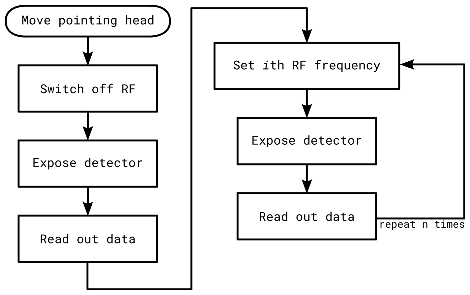
Figure 3 Schematic representation of the acquisition process for a single hypercube. For every acoustic frequency n, the corresponding RF frequency i needs to be set.

The NO₂ camera uses a different method to create images of the NO₂ field. Instead of scanning the scene, Dekemper et al. (2016) proposed capturing complete images of the scene, but one wavelength at a time. The imaging quality is that of a real imaging system, offering a higher spatial sampling than fiber-bundle-based diffraction grating spectrometers, while temporal variations can still be tracked in successive images. One drawback lies in the perturbations caused by the spectra recorded by pixels that have seen objects moving during the cube acquisitions. Additionally, the optical throughput of a telecentric AOTF-based imager is lower than that of a diffraction grating spectrometer, yielding a lower SNR. This lower SNR allows observations with SZA up to 90° while maintaining the per-frame exposure at 1 s, but twilight observations would require adaptations.

On the other hand, this method has the advantage that images are acquired from the start. Pointing errors are easily corrected by using features in the pictures. More importantly, highly dynamic processes can be detected and monitored, especially when the camera is focusing on a limited number of wavelengths. Whereas diffraction grating-based systems automatically record the complete spectrum for their design bandwidth, AOTF-based systems allow the user to cherry-pick the wavelengths of interest: there is no fixed sequence of wavelengths required. Therefore, a wavelength band of interest can be defined for any species, and only this wavelength band will be sampled by the camera. In the context of satellite retrievals, Ruiz Villena et al. (2020) proved the feasibility of discrete-wavelength DOAS using only 10 carefully chosen wavelengths and reaching correlations above 99 % with the operational products from OMI and TROPOMI. The power plant campaign described by Dekemper et al. (2016) follows a slightly different approach based on eight wavelengths. This way, the number of images required can be decreased, bringing the time for a single scene measurement below 10 s.

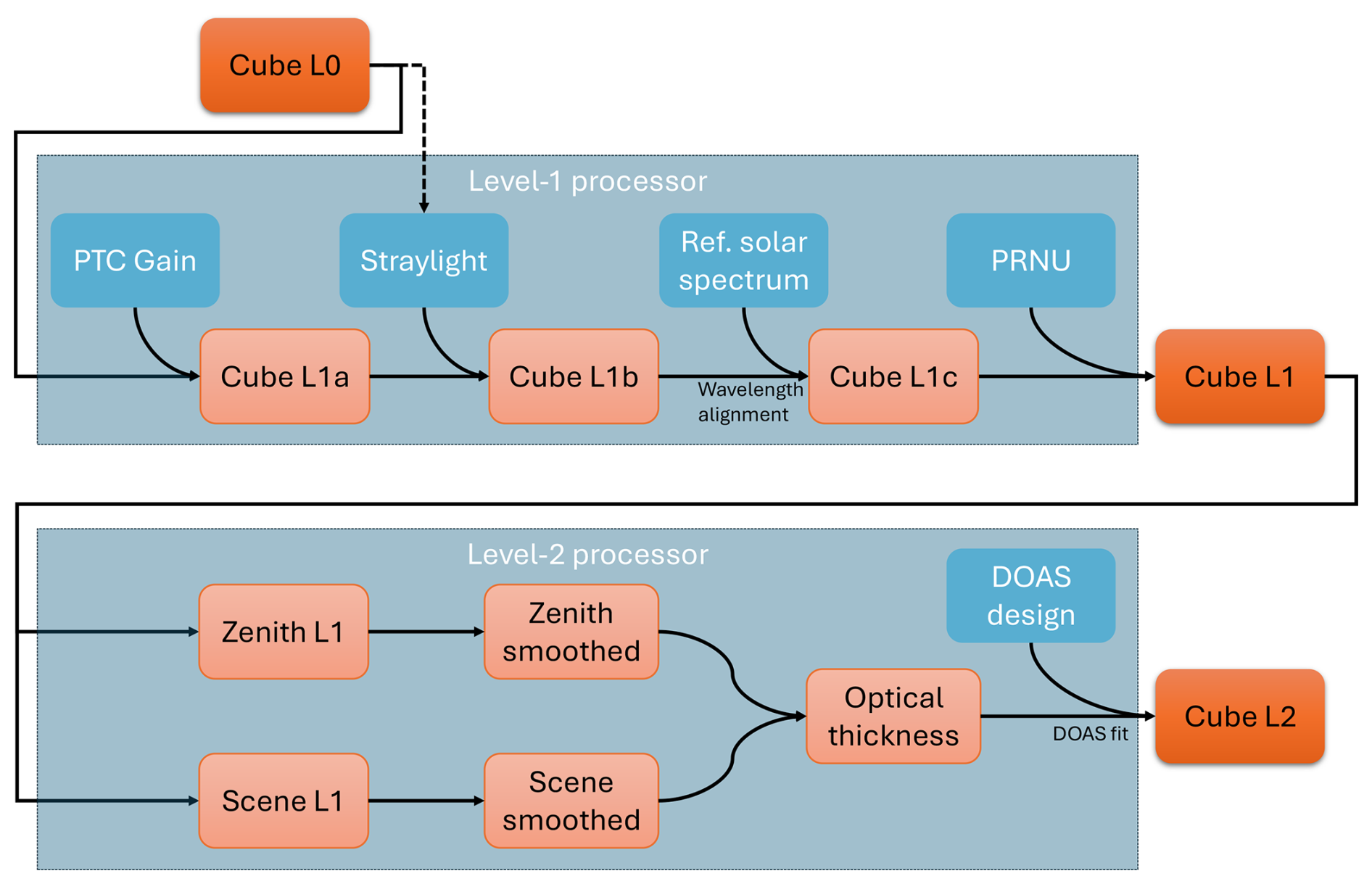
Figure 4 Overview of the data processing for the retrieval of NO₂ dSCDs (Level-2 data) from the NO₂ camera acquisitions (Level-0 data).

3 NO₂ camera data processing

3.1 Overview

The data processing for the NO₂ camera is organized into Level-0 (raw spectra), Level-1 (calibrated spectra) and Level-2 (retrieval outcome). The main processing steps are shown in Fig. 4, and more details are provided in the next sections.

3.2 Level-1 processor

The first step of the Level-1 processor (L1P) is to convert the acquired raw data from digital number to electron count. A preliminary calibration experiment was performed in order to compute a photon transfer curve (PTC) and derive its parameters, following Janesick (2007). At gain parameter 200 (×0.1 dB), used during the campaign, our computations gave a gain of 0.0793 e⁻ DN⁻¹, a read noise of 1.206 e⁻ and a fixed pattern noise (FPN) of 0.2 %, confirming the vendor characteristics. The PTC showed that the CMOS detector's response is very close to linear; thus, the conversion to electrons amounts to a simple multiplication by the gain (and a detector offset that can be ignored thanks to the following stray light removal). The stray light images (acquired at least once per hyperspectral cube) are also converted to electrons (e⁻) and subtracted pixel by pixel from the target images. To maintain physical interpretability, all values under 1 e⁻ are forced to 1 e⁻ (i.e., close to the read noise).

An illustration of this stray light removal is shown in Fig. 5. The intensity of stray light observed is typically less than 10 % of the scene intensity, except in a small region of about 70 × 70 pixels. This region changes slightly depending on the pointing and solar angles, and its stray light may reach values comparable to the real stray light-corrected intensity (especially on scenes with less light in their lower part and at wavelengths under 435 nm).

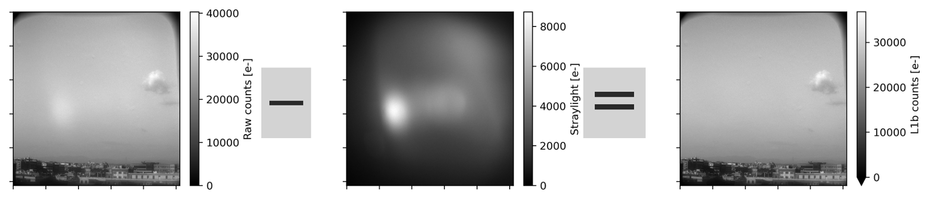
Figure 5 Illustration of stray light removal. Note the smaller values in the color scale for the central image, which was captured with the AOTF turned off.

The optical wavelength filtered by the AOTF at a given acoustic frequency is known to depend on the crystal temperature, varying by about 0.1 nm per K. Although this variation can be computed and corrected for, a more precise wavelength registration is obtained by detecting the Fraunhofer lines, which are clearly visible in the measured spectra. For this purpose, the average intensity at the 64 × 64 central pixels of the cube is compared to the convolved solar reference spectrum, the same as in Sect. 2.2. The wavelength correction function is the solution of a non-linear optimization problem whose search space consists of all increasing affine functions of the wavelength, with the identity function as the starting point. The score that is minimized is the mean absolute difference of logarithms, after subtracting broadband differences as in Sect. 2.2.

The final step in Level-1 processing is to correct for pixel response non-uniformity (PRNU), a type of instrumental bias where some pixels would show a different sensitivity from others when exposed to the same input signal. Because this PTC analysis showed no significant non-linearity in the instrument's response, we could use the PTC data to model the PRNU with a simple per-pixel scaling factor independent of the wavelength and of the light intensity, even though these hypotheses may not be fully correct. This scaling factor is computed on one reference zenith cube, typically the same as that used in Level-2 data processing, taking the per-pixel average intensity across all wavelengths. Note that the first step of Level-2 data processing (see below) is to compute the ratio between the zenith and scene intensities. Therefore, regardless of the choice of linear scaling used in the PRNU correction, it will not have any impact on the Level-2 product. That correction can thus be considered as a cosmetic step, only useful when displaying Level-1 images.

Putting it all together, the Level-1 intensity in electrons I_L1 at wavelength λ and pixel i,j is computed as

$$\begin{array}{}\text{(1)}& I_{\text{L1}}(\mathit{\lambda },i,j)={\displaystyle \frac{max\left(\mathrm{1},GS(\stackrel{\mathrm{̃}}{\mathit{\lambda }},i,j)-G{S}_{\mathrm{0}}(i,j)\right)}{\mathrm{PRNU}(i,j)}},\end{array}$$

where $\stackrel{\mathrm{̃}}{\mathit{\lambda }}$ is the nominal wavelength, before alignment; λ is the truly measured wavelength after alignment: $\mathit{\lambda }=\stackrel{\mathrm{̃}}{\mathit{\lambda }}+\mathrm{\Delta }\left(\stackrel{\mathrm{̃}}{\mathit{\lambda }}\right)$, where Δ is a smooth function of the nominal wavelength optimizing the alignment of the Fraunhofer structure; G is the detector's gain; S is the L0 signal intensity in digital numbers; S₀ is the L0 stray light signal intensity in digital numbers (i.e., with the AOTF off); I_L1 is the Level-1 signal intensity in electrons; and PRNU(i,j) is the PRNU factor.

In addition to the calibrated light intensity, a pointing map is computed as well, assigning an elevation and azimuth viewing angle to each pixel of the Level-1 image. This map is calibrated using prominent features, such as buildings and mountains, whose viewing angles were determined from publicly available topographic maps and/or aerial photos. Its precision is expected to be around 0.05° (one pixel).

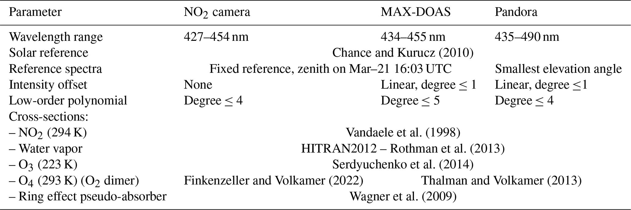
Chance and Kurucz (2010)Vandaele et al. (1998)Rothman et al. (2013)Serdyuchenko et al. (2014)Finkenzeller and Volkamer (2022)Thalman and Volkamer (2013)Wagner et al. (2009)

Table 3 Parameters and cross-sections used in the DOAS retrieval for each smoothed pixel of the NO₂ camera measurements and for both reference instruments.

3.3 Level-2 processor

The retrieval of NO₂ differential slant column densities (dSCDs) from hyperspectral cubes is based on the well-established DOAS (differential optical absorption spectroscopy; see Platt and Stutz, 2008) method, which relies on the Beer–Lambert law:

$$\begin{array}{}\text{(2)}& I\left(\mathit{\lambda }\right)=I_{\mathrm{0}}\left(\mathit{\lambda }\right)\cdot \exp \left(-\sum _{k=\mathrm{1}}^K{S}^k\left(\mathit{\lambda }\right)c_k\right),\end{array}$$

where I(λ) is the measured spectrum of interest, after extinction in the atmosphere; I₀(λ) is the zenith spectrum, an approximation of the spectrum at the top of the atmosphere; S^k(λ) is the absorption cross-section of the species k, depending on the wavelength [${\mathrm{cm}}^{\mathrm{2}}\mathrm{molec}{.}^{-\mathrm{1}}$]; and c_k is the dSCD of the species k [$\mathrm{molec}.{\mathrm{cm}}^{-\mathrm{2}}$].

The principle of the DOAS method is to focus on high-frequency spectral structures in this equation, approximating the low-frequency structures (such as instrumental effects, aerosol scattering, etc.) with a low-order polynomial $P_{\le n}\left(\mathit{\lambda }\right)={\sum }_k{p}_k{\mathit{\lambda }}^k$. Defining the optical thickness τ(λ) as the log-ratio, the previous equation becomes

$$\begin{array}{}\text{(3)}& \mathit{\tau }\left(\mathit{\lambda }\right)\equiv \log {\displaystyle \frac{I_{\mathrm{0}}\left(\mathit{\lambda }\right)}{I\left(\mathit{\lambda }\right)}}=\sum _{k=\mathrm{0}}^n{p}_k{\mathit{\lambda }}^k+\sum _{k=\mathrm{1}}^K{S}^k\left(\mathit{\lambda }\right)c_k.\end{array}$$

Writing {λ_l}_l=1…L for the wavelengths at which the optical thickness was measured and defining the DOAS design matrix as

$$\begin{array}{}\text{(4)}& \begin{array}{rl}\mathbf{A}& \equiv \left(\begin{array}{ccccccc}\mathrm{1}& {\mathit{\lambda }}_{\mathrm{1}}& \mathrm{\cdots }& {\mathit{\lambda }}_{\mathrm{1}}^n& S^{\mathrm{1}}\left({\mathit{\lambda }}_{\mathrm{1}}\right)& \mathrm{\cdots }& S^K\left({\mathit{\lambda }}_{\mathrm{1}}\right)\\ \mathrm{1}& {\mathit{\lambda }}_{\mathrm{2}}& \mathrm{\cdots }& {\mathit{\lambda }}_{\mathrm{2}}^n& S^{\mathrm{1}}\left({\mathit{\lambda }}_{\mathrm{2}}\right)& \mathrm{\cdots }& S^K\left({\mathit{\lambda }}_{\mathrm{2}}\right)\\ \mathrm{⋮}& \mathrm{⋮}& \mathrm{⋮}& \mathrm{⋮}& \mathrm{⋮}& \mathrm{⋮}& \mathrm{⋮}\\ \mathrm{1}& {\mathit{\lambda }}_L& \mathrm{\cdots }& {\mathit{\lambda }}_L^n& S^{\mathrm{1}}\left({\mathit{\lambda }}_L\right)& \mathrm{\cdots }& S^K\left({\mathit{\lambda }}_L\right)\end{array}\right)\\ & \in {\mathbb{R}}^{L\times (\mathrm{1}+n+K)},\end{array}\end{array}$$

Eq. (3) can be rewritten as a simple linear fit for each pixel (i,j):

$$\begin{array}{}\text{(5)}& \mathbf{A}\cdot \mathit{x}(i,j)=\mathit{\tau }(i,j)\forall i,j,\end{array}$$

whose unknown x(i,j) are the concatenation of the polynomial coefficients p(i,j) and the dSCDs c(i,j) at pixel (i,j).

For the NO₂ camera, the value of the measured response (optical thickness τ(i,j)) and of these unknown variables x(i,j) will vary from pixel to pixel, whereas the design matrix A is common to all pixels. As noted earlier, the per-pixel FoV is around 0.045°. In order to make it comparable to the reference instruments (∼ 0.3 ×1° for MAX-DOAS and ∼ 1.5 × 1.5° for Pandora), a box smoothing is applied to the zenith and the scene using a uniform 7 × 23 or 33 × 33 pixel kernel on each Level-1 intensity map before computing the optical thickness.

The DOAS fitting settings are very close to the recommendations for the NO2VIS-SMALL analyses during the CINDI-3 intercomparison campaign (https://frm4doas.aeronomie.be/index.php/cindi-3, last access: 17 October 2025). A notable difference is the wavelength range (427–454 nm versus 411–445 nm), which we kept a bit shorter to limit the acquisition time and which we extended slightly towards longer wavelengths to include additional NO₂ absorption features (visible in Fig. 6). The settings are summarized in Table 3, and an example of the retrieval output is shown in Fig. 6.

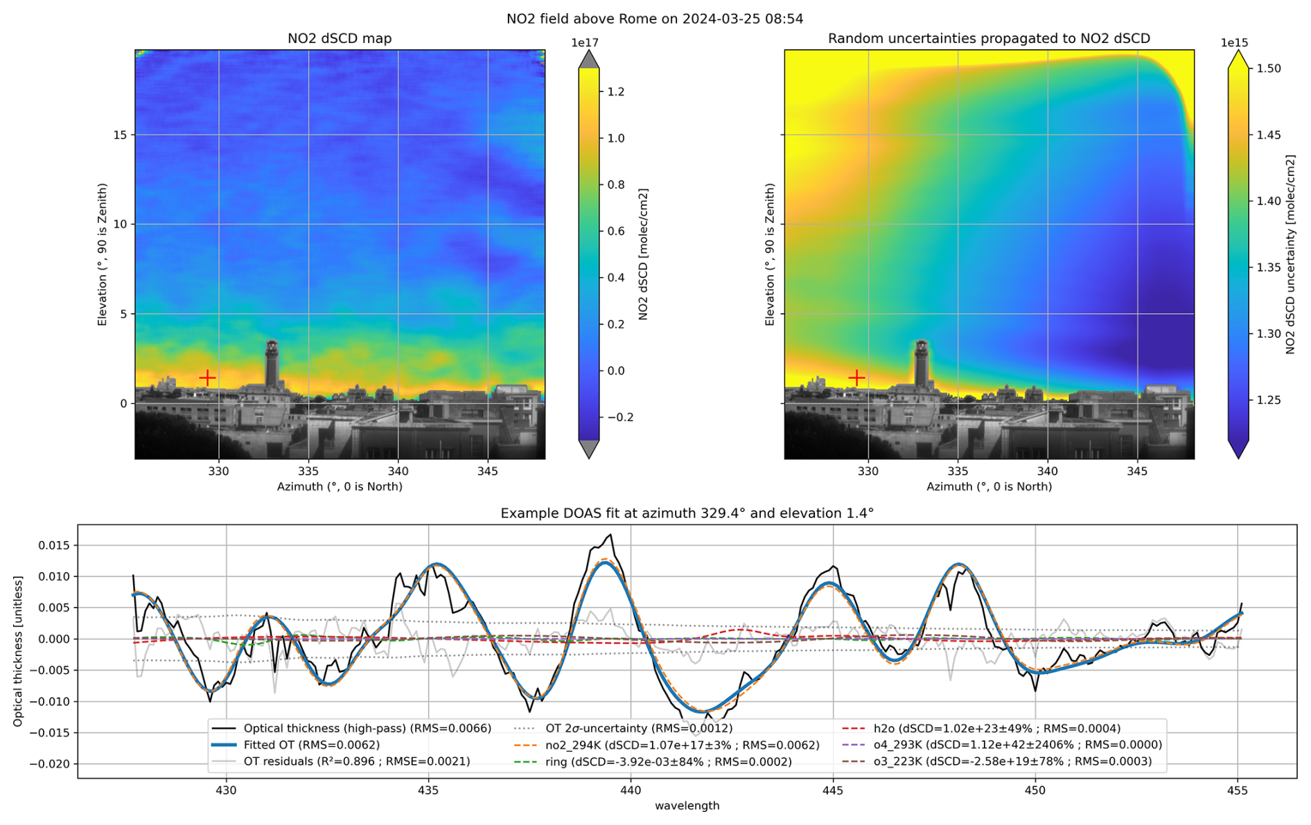
Figure 6 Example of output from NO₂ camera retrieval, acquired in Rome on 25 March, from 08:55 to 09:01 UTC. The top-left panel shows the map of NO₂ dSCDs retrieved for each pixel, whereas the top-right panel shows its estimated uncertainties. In order to give finer spatial context, the pixels under the horizon for both images show the landscape (from the Level-1 data at 455 nm). The bottom panel shows the details of the DOAS fit for one example pixel, marked with a red cross in the top images.

3.4 Characterization of uncertainties

Considering the NO₂ dSCD as the measurand, we characterize the uncertainty on its estimated values by uncertainty propagation through the measurement model described in the previous sections, starting at its input quantities. In a first attempt, only the random uncertainty in the intensity measurements is considered.

The main random uncertainties affecting the signal (Level-1) measurements come from the CMOS sensor. Following the PTC analysis mentioned earlier, three independent noise components are considered: the read noise, the Poisson shot noise and the fixed pattern noise. The uncertainty associated with a CMOS output of s electrons is then

$$u_{\text{CMOS}}\left(s\right)=\sqrt{{\mathit{\sigma }}_{\text{RN}}^{\mathrm{2}}+s+p_{\text{FPN}}^{\mathrm{2}}{s}^{\mathrm{2}}},$$

where ${\mathit{\sigma }}_{\text{RN}}^{\mathrm{2}}=\mathrm{0.6}$ e⁻ is the variance of the read noise, s is the variance of the Poisson shot noise and p_FPN=0.2 % is the proportion of FPN. This is valid for the target images as well as the stray light images. At the typical values of the input signal (i.e., 5000 to 60 000 e⁻), the read noise is negligible compared to the shot noise, so we ignore it for the sake of simplicity. As for the FPN, its maximal contribution is obtained when the input signal is highest. For an input of 60 000 e⁻, the uncertainty including 0.2 % FPN amounts to 273 e⁻ versus 245 e⁻ without FPN, which proves that the FPN impact is limited or even negligible depending on the signal level. Moreover, the subtraction of stray light and the division by the PRNU map in Eq. (1) have the side effect of removing the additive and the multiplicative components of FPN, respectively. Potentially remaining FPN would be much smaller and come from non-linear effects, which are hard to characterize. For this reason, FPN is also ignored, and the standard uncertainty of the Level-1 signal, u_L1, is

$$u_{\text{L1}}(\mathit{\lambda },i,j)\simeq {\displaystyle \frac{\mathrm{1}}{\text{PRNU}(i,j)}}\sqrt{GS(\stackrel{\mathrm{̃}}{\mathit{\lambda }},i,j)+G{S}_{\mathrm{0}}(i,j)}.$$

In this equation, G is again the detector's gain, S the L0 signal intensity and S₀ the L0 stray light signal as defined in Eq. (1). While we do expect close values of $I_{\text{L1}}(\mathit{\lambda },i,j)$ for neighboring wavelengths and pixels, we assume that their measurement errors are statistically independent. Therefore, we do not consider the covariance structure among the measurement errors at different pixels and wavelengths in the signal. We also hypothesize that the target and zenith cubes are independent. We are aware of the limiting aspect of these assumptions: we will address them in future developments, and an empirical approach is proposed for the campaign results presented in this work. Propagating these random uncertainties in the definition of optical thickness (including the preliminary box-smoothing intensities with size k×k) gives the uncertainty on the optical thickness, u_τ:

$$\begin{array}{}\text{(6)}& \begin{array}{rl}{u}_{\mathit{\tau }}(\mathit{\lambda },i,j)& =\sqrt{{\displaystyle \frac{u_{\text{L1}}^{\mathrm{2}}(\mathit{\lambda },i,j)}{k^{\mathrm{2}}{I}_{\text{L1}}^{\mathrm{2}}(\mathit{\lambda },i,j)}}+{\displaystyle \frac{u_{z,\text{L1}}^{\mathrm{2}}(\mathit{\lambda },i,j)}{k^{\mathrm{2}}{I}_{z,\text{L1}}^{\mathrm{2}}(\mathit{\lambda },i,j)}}}\\ & \simeq {\displaystyle \frac{\mathrm{1}}{k}}\sqrt{{\displaystyle \frac{\mathrm{1}}{I_{\text{L1}}(\mathit{\lambda },i,j)}}+{\displaystyle \frac{\mathrm{1}}{I_{z,\text{L1}}(\mathit{\lambda },i,j)}}},\end{array}\end{array}$$

where I_z,L1 and u_z,L1 are, respectively, the intensity and uncertainty of the zenith measurements. The last approximation is valid when the stray light intensity is small compared to the target image.

Assuming that the DOAS design matrix A is perfectly known, the uncertainty on τ(x,y) propagates to the dSCDs and polynomial coefficients as the following covariance matrix:

$$\begin{array}{}\text{(7)}& {\mathrm{\Sigma }}_{\mathit{x}(i,j)}={\left({\mathbf{A}}^{\top }\mathrm{diag}\left(\mathrm{1}/{\mathit{u}}_{\mathit{\tau }}^{\mathrm{2}}(i,j)\right)\mathbf{A}\right)}^{-\mathrm{1}}.\end{array}$$

Returning the full covariance structure for each pixel is not practical for the data users; therefore, only the square root of the diagonal terms is reported:

$$\begin{array}{}\text{(8)}& {\mathit{u}}_{\mathit{x}}(i,j)=\sqrt{\mathrm{diag}\left({\mathrm{\Sigma }}_{\mathit{x}(i,j)}\right)}.\end{array}$$

This produces a one-dimensional uncertainty estimate for the NO₂ dSCD at each pixel, which we can display in a map similarly to the dSCDs themselves, as shown in Fig. 6. The residuals of the DOAS spectral fit show some non-random structure and are regularly larger than the estimated uncertainty on optical thickness. This shows that our estimation underestimates the true total uncertainty, which was expected because we ignored the systematic contributions.

An in-depth assessment of systematic uncertainties is outside the scope of this paper. However, some preliminary analyses showed that a small error of 0.01 nm in the wavelength alignment might propagate to an error of 5 ×10¹⁵ molec. cm⁻² on the NO₂ dSCD. Therefore, we expect the wavelength alignment to be a major contributor to the NO₂ dSCD uncertainties. Improper stray light removal might be another important source of systematic uncertainty, as the optical thickness would be multiplied by a factor close to $(\mathrm{1}-I_{\text{stray}}(\mathit{\lambda })/I_{\mathrm{0}}(\mathit{\lambda }\left)\right)$ (Platt and Stutz, 2008, p. 327), hence also influencing all dSCDs. If the remaining stray light intensity in the Level-1 image is about 2 % (positive or negative), this could impact the NO₂ dSCD by up to $\pm \mathrm{4}\times {\mathrm{10}}^{\mathrm{15}}$ molec. cm⁻². Finally, Vandaele et al. (1998) report an uncertainty ≤ 3 % on the NO₂ cross-section, which might also contribute to the dSCD uncertainty. A full error budget for the instrument will be worth a separate publication when it is completed.

4 Campaign in Rome

4.1 Objectives

In Rome, the Atmospheric Physics Laboratory (APL) of Sapienza University hosts the BAQUNIN (Boundary-layer Air Quality-analysis Using Network of INstruments) supersite, where several ground-based instruments are available that monitor the boundary layer air quality (Iannarelli et al., 2022). This urban observatory is equipped to host ground-based instruments such as the NO₂ camera for intercomparison/intercalibration campaigns. It was selected as the location for a first urban test campaign in a challenging environment showing strong spatial and temporal variations.

The goal of the measurement campaign in Rome is to validate the correctness of the NO₂ camera retrievals with two state-of-the-art remote sensing instruments: a Pandora and a MAX-DOAS instrument, described hereafter. Both of these reference instruments measure dSCDs. By performing a light path assessment (e.g., using O₄ absorption) and the inversion of NO₂ concentration vertical profiles, their results can typically be converted to NO₂ concentrations. As this paper focuses on the measurement and operational principle of the NO₂ camera rather than on the processing of the results, only NO₂ dSCDs are compared between the different reference instruments and the NO₂ camera. The light path assessment, the inversion of the vertical profile and the resulting NO₂ concentration have a high priority on the NO₂ camera roadmap through a pending integration into the FRM4DOAS framework (Van Roozendael et al., 2024) but are outside the scope of this paper.

4.2 Reference NO₂ remote sensing instruments

4.2.1 MAX-DOAS

The MAX-DOAS instrument used for the campaign is a SkySpec-2D system by Airyx. This system was acquired by CNR-ISAC in 2021 and operated from the CIRAS (CNR Isac Rome Atmospheric obServatory) in the CNR research area of Tor Vergata since September 2021. The instrument is composed of a telescope (installed outdoors), a spectrometer unit and a measurement PC. The spectrometer is connected to the telescope via an optical fiber. The spectrometer unit contains two spectrometers that simultaneously acquire the spectra in the UV and VIS spectral ranges at a high spectral resolution. The prism telescope covers elevation angles from −10 to 190°. The 2D model allows the user to measure at different azimuth angles.

The instrument was transferred from CIRAS to BAQUNIN and installed on the roof of APL, on another platform about 5 m away and lower than the Pandora and NO₂ camera. The measurements were analyzed using QDOAS software and the same parameters as in Pettinari et al. (2022). These parameters are summarized in Table 3 for convenience.

4.2.2 Pandora

Pandora-2S instruments are fiber-fed hyperspectral spectrometers mounted on a microprocessor-controlled azimuth/elevation tracker and manufactured by SciGlob LLC (Elkridge, MD, USA). They are regrouped in the Pandonia Global Network (PGN), which is co-funded by NASA and ESA and operated by LuftBlick OG (Innsbruck, Austria). The instrument present at the BAQUNIN-APL supersite has identifier PAN#117.

For each day of the PAN#117 measurements, a set of Level-2 fit files is produced by the PGN centralized processing, each corresponding to a specific measurement mode and target species. Because the campaign focused on NO₂, the “nvh3” data product was analyzed. A detailed description of the fit, its parameters and its outputs is provided in Cede et al. (2025) and summarized in Table 3 for convenience. The uncertainty estimates of the retrieved NO₂ dSCDs were obtained by combining in quadrature their independent, structured and common uncertainties.

4.2.3 Differences in retrievals parameters

The retrieval parameters of the different instruments are listed in Table 3. Even though differences in retrieval settings can cause inter-instrumental differences, we have opted to keep the settings of the reference instruments the same as in earlier published results.

The summary in Table 3 underlines some inter-instrumental differences in DOAS parameters. This results from a will to reuse prescribed settings from published results from each instrument separately. This is a potential cause for inter-instrumental differences in retrieved dSCDs.

In particular, the agreement on a reference spectrum is crucial to compare dSCDs from several DOAS instruments. The NO₂ camera and the MAX-DOAS used a fixed zenith reference acquired on the 21 March at 16:00 UTC for all their dSCDs. The Pandora, on the other hand, relies on centralized processing within PGN to obtain an NO₂ dSCD. It is thus based on a sequential reference, defined as the spectrum taken at the lowest viewing elevation angle during each azimuthal scan (Cede et al., 2025, Product nvh3). Most of its dSCDs are then expected to be negative, requiring a post-processing step for comparability.

The difference in reference between the instruments could be compensated for by computing a correction term for each Pandora azimuthal scan and adding it to all dSCDs in the scan. To compute this term, we compared the Pandora zenith dSCD during each scan with the corresponding (time-interpolated) retrieval of the MAX-DOAS. Their difference was added to all dSCDs at all viewing elevation angles in the same azimuthal scan from Pandora. When the scan contains several zenith observations, the averaged difference was used. This correction was also accounted for in the uncertainty estimates.

The difference in O₄ cross-section is not expected to have a strong influence on the comparison results because we focus on the NO₂ dSCD without performing the inversion to concentration profiles.

Finally, another significant difference between the instruments is the longer wavelength range used in the Pandora retrievals. We do believe it has an impact on the comparison results: this longer range is expected to include photons with a longer optical path, hence increasing the Pandora's dSCDs. However, we preferred to adhere to the well-validated operational settings of the international PGN to retain its value as a reference instrument.

4.3 Acquisition plan

Four primary azimuth angles were selected for the actual measurement campaign: 27, 124, 130 and 340°. Sample images showing the scenes in the different azimuth directions are shown in Fig. 7. Each different azimuth represents a different type of environment. In the directions of 27 and 340°, the area is mostly residential, whereas 124 and 130° are mixed residential and industrial zones. For the latter azimuth directions, the optical path is limited by the mountains for parts of the image. The tower that is clearly visible in the image taken in the 340° direction was used to calibrate the pointing of each instrument.

After a calibration and test phase at the beginning of the campaign, the Pandora and MAX-DOAS instruments started sampling the NO₂ field inside the field of view of the NO₂ camera. This allows the user to reconstruct a two-dimensional NO₂ dSCD map for each instrument. Figure 7b highlights these sample points for both the MAX-DOAS and Pandora.

In both azimuth and elevation, Pandora samples every 1°. A denser spatial sampling is not necessary, as the field of view of the Pandora instrument is roughly a circle of 1.5° diameter. The MAX-DOAS instrument has a field of view of around 0.3° vertically by 1° horizontally. Therefore, a measurement was taken every 0.5° in elevation angle and every 1° horizontally.

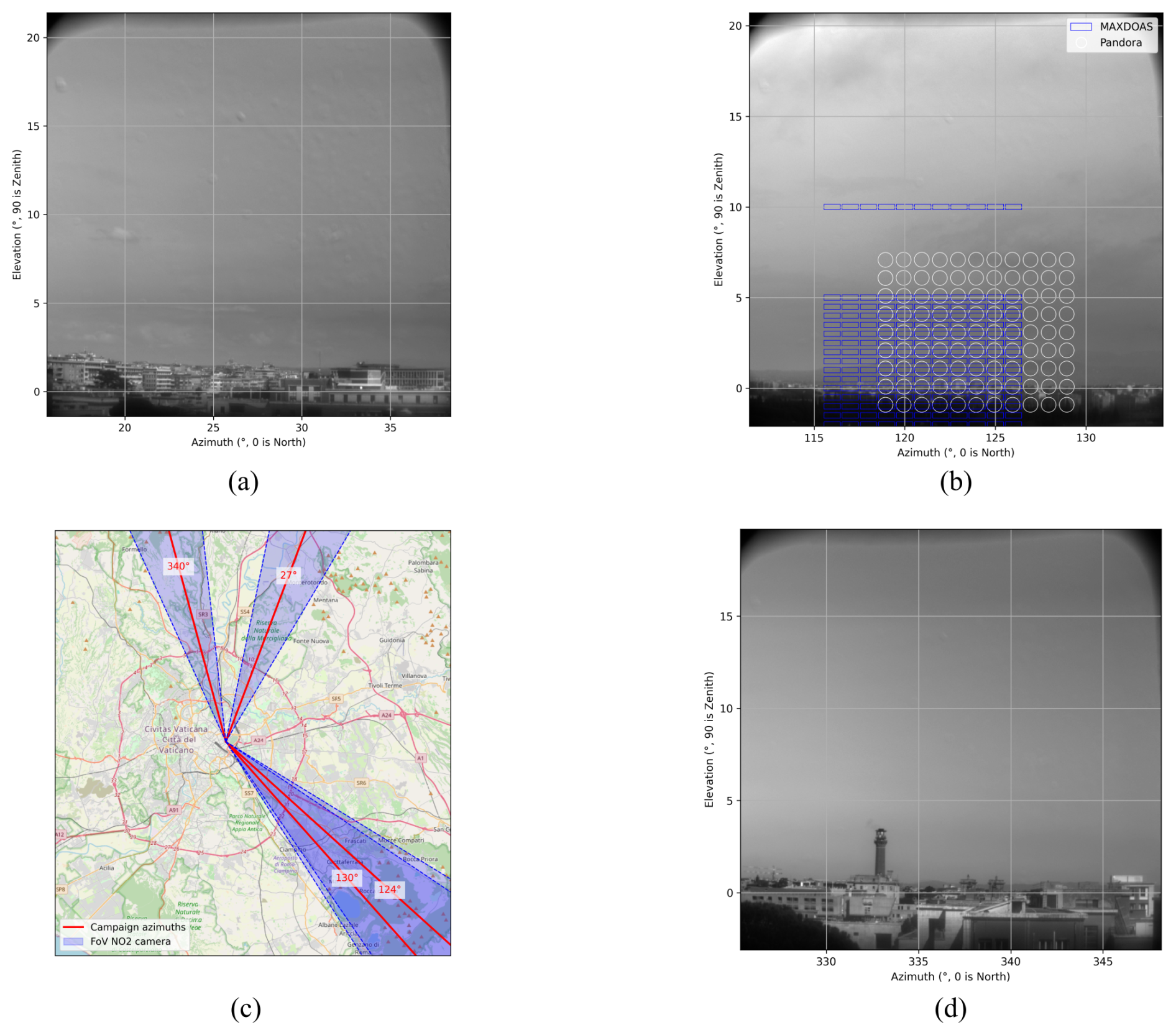
Figure 7 Representative spectral images (at 460 nm) of the main azimuth directions observed during the campaign, with (a) 27°, (b) 124° and (d) 340°. Each one covers a different type of environment. In addition, panel (b) shows the spatial sampling of the Pandora and MAX-DOAS instruments within the field of view of the NO₂ camera. For the sake of readability, this is not shown on the other scenes. Panel (c) shows the four main azimuths used during the measurement campaign. The shaded area in blue shows the field of view of the camera. For 124 and 130°, the camera takes pictures in the directions of 126 and 128°, respectively. This allows us to have more comparison points with the other instruments. Map data in panel (c) © OpenStreetMap contributors, 2025. Distributed under the Open Data Commons Open Database License (ODbL) v1.0.

5 Campaign results

5.1 Comparison methodology

For every Pandora and MAX-DOAS measurement, the closest NO₂ camera pixel in space is determined. For this pixel, the dSCD value is compared to the results of the Pandora and MAX-DOAS instruments. Both in azimuth and elevation, a tolerance of 0.1° was allowed. When the pointing correction is applied correctly, the elevation angle and the time difference remain the two parameters that influence the quality of the correlation the most, as we will now discuss.

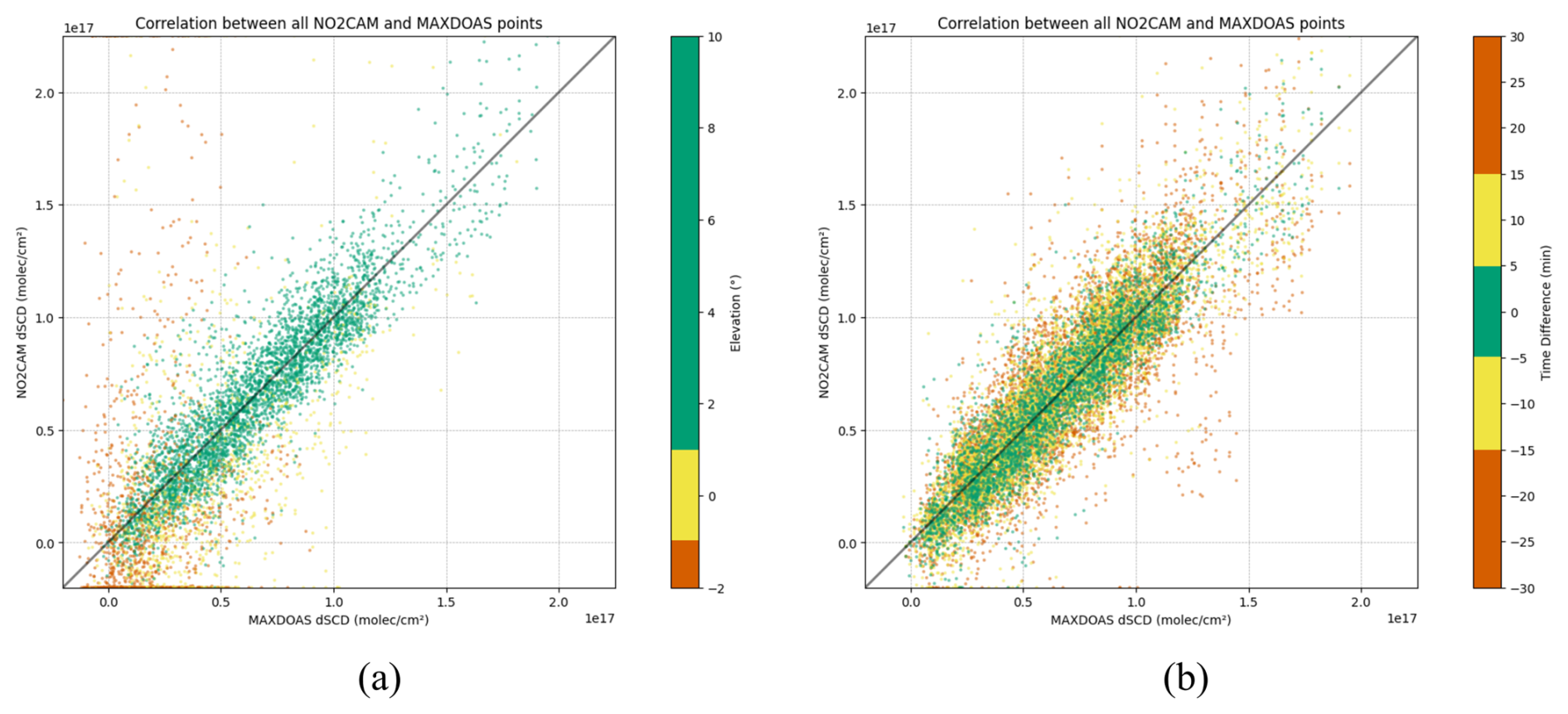
Figure 8 Comparing dSCDs between the NO₂ camera and the MAX-DOAS instrument shows the strong impact of measurements under the horizon and of large differences in measurement timestamps. Panel (a) shows that the low elevation points differ more significantly from the diagonal than the points above 1° (green versus red). Panel (b) focuses on elevation above 1° and shows that the allowed time difference for the comparison strongly influences the results: smaller time differences have better correspondence (green versus red). In both panes, values outside the viewing window are clipped to the viewing window border.

Figure 8a shows all the dSCDs measured by the MAX-DOAS instrument and their corresponding dSCDs retrieved by the NO₂ camera. For this comparison, a maximum time difference of 30 min is allowed between the MAX-DOAS and the NO₂ camera measurement. The different measurement points are colored according to the elevation angle at which they are measured. Ideally, all measured points would lie on the diagonal: both dSCDs would be equal in this case. The dots colored in red indicate elevation angles well below the horizon (−1°). The dots colored in yellow are measurement points between −1 and 1°. The green dots show the measurements for elevation angles higher than 1°. Values outside the limits of the axes are clipped to the axis limit. The different colors demonstrate that, for low elevation angles, the correlation between MAX-DOAS and the NO₂ camera is significantly worse than for higher elevation angles. As the figure for the Pandora instrument is very similar but with fewer data points available, this image is not shown here. This is due to the presence of buildings (visible in Fig. 7), inducing a much shorter light path for some instruments. Because the instruments were located a few meters away from each other (including a difference in elevation for MAX-DOAS), the parallax error leads to differences in the observed scenes. For the remainder of the paper, we will remove from the comparison all points that are at or below 1°.

For Fig. 8a, a maximum of 30 min was allowed between the MAX-DOAS and the NO₂ camera measurement. This time difference has a significant impact on the comparison between the instruments. Figure 8b illustrates this influence. Here, only elevation angles above 1° are shown. The less stringent the time requirements become, the more spread out the values are. Values outside the limits of the axes are again clipped to the axis limit. This illustrates that the NO₂ field presents dynamic patterns at the scale of minutes. Therefore, we restrict the time tolerance to ±5 min for the comparisons in this paper.

5.2 Comparison results

Before comparing the NO₂ camera with each reference instrument, we first present a baseline comparison between the MAX-DOAS and the Pandora results. The purpose of this analysis is to set a baseline for the quality of the main comparisons involving the NO₂ camera. Even though both reference instruments have already been extensively validated, we do expect some differences in the results because of the imperfect time synchronization and the different DOAS settings, as explained in Sect. 4.2.3. A simple difference and a linear regression were used to characterize the relation between the Pandora and MAX-DOAS dSCDs after applying the data filters discussed in the previous section. These statistics were calculated globally for all azimuth directions, and outliers outside the interval [$-\mathrm{2}\times {\mathrm{10}}^{\mathrm{16}},\mathrm{2}\times {\mathrm{10}}^{\mathrm{17}}$] $\mathrm{molec}.{\mathrm{cm}}^{-\mathrm{1}}$ were excluded for the regression.

Due to small differences in the scanning schedule of the Pandora and MAX-DOAS instruments, this direct comparison includes only 69 measurement points, much less than the comparisons involving the NO₂ camera. The results, presented in Fig. 9, show a root-mean-square error (RMSE) of 7×10¹⁵ $\mathrm{molec}.{\mathrm{cm}}^{-\mathrm{2}}$ and a mean bias of 2×10¹⁵ $\mathrm{molec}.{\mathrm{cm}}^{-\mathrm{2}}$. The line of best fit has a slope of 0.99 ± 0.04 and an R² value of 0.97. In this direct comparison, we would actually expect a regression slope above 1 due to the longer wavelength range used in the Pandora instrument. However, the very limited number of points might have prevented us from observing it, as shown by the confidence interval.

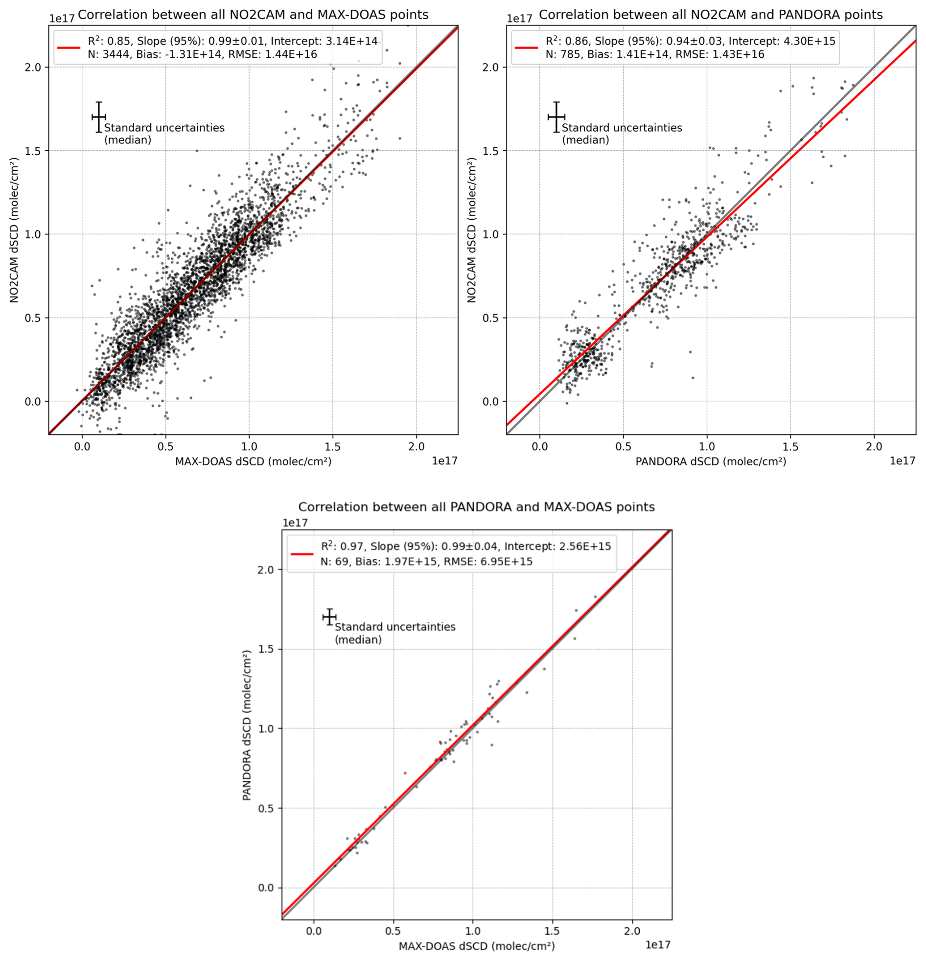
Figure 9 Scatterplots comparing the NO₂ camera with the MAX-DOAS (upper-left panel) and Pandora (upper-right panel) instruments, including a linear regression for each. Measurement points were filtered to elevations above 1° (strictly) and a time difference under 5 min. The lower panel shows a direct comparison of the MAX-DOAS and Pandora instruments using the same filters, which serves as a baseline.

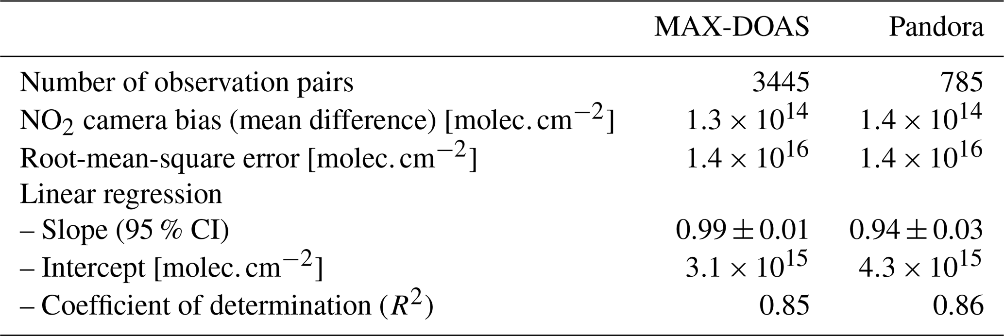
The main analysis compared the NO₂ camera to each reference instrument, computing a simple difference and a linear regression with the same methodology as the baseline analysis. The summary statistics are detailed in Table 4. In particular, the root-mean-square error (RMSE) obtained is 1.4×10¹⁶ $\mathrm{molec}.{\mathrm{cm}}^{-\mathrm{2}}$ compared to both references, and the mean bias is very small, at 1.3×10¹⁴ $\mathrm{molec}.{\mathrm{cm}}^{-\mathrm{2}}$ (MAX-DOAS) and 1.4×10¹⁴ $\mathrm{molec}.{\mathrm{cm}}^{-\mathrm{2}}$ (Pandora). The regressions and the corresponding scatter plots are shown in Fig. 9. The regression slope obtained is 0.99 for the comparison with MAX-DOAS. For Pandora, the slope is 0.94, which is significantly smaller than unity. A possible explanation is Pandora's longer wavelength range.

Table 4 Summary statistics for the comparison of the camera's NO₂ dSCDs to each reference instrument on all common retrievals from the campaign.

5.3 Imaging results

Example images of the dSCDs measured in the different azimuthal directions are shown in Fig. 10. In these figures, fine structures in the NO₂ field can be distinguished. As expected, lines of sight grazing the horizon capture much higher NO₂ dSCDs. The imaging quality of the NO₂ camera also reveals horizontal and vertical gradients. An interesting case is, for instance, the enhancement on the left side of Fig. 10b, which should be further investigated. In addition, some figures show artifacts in the upper part of the image. These artifacts are created by the moving clouds or aerosols, whereas the lower region of the image is left unaffected.

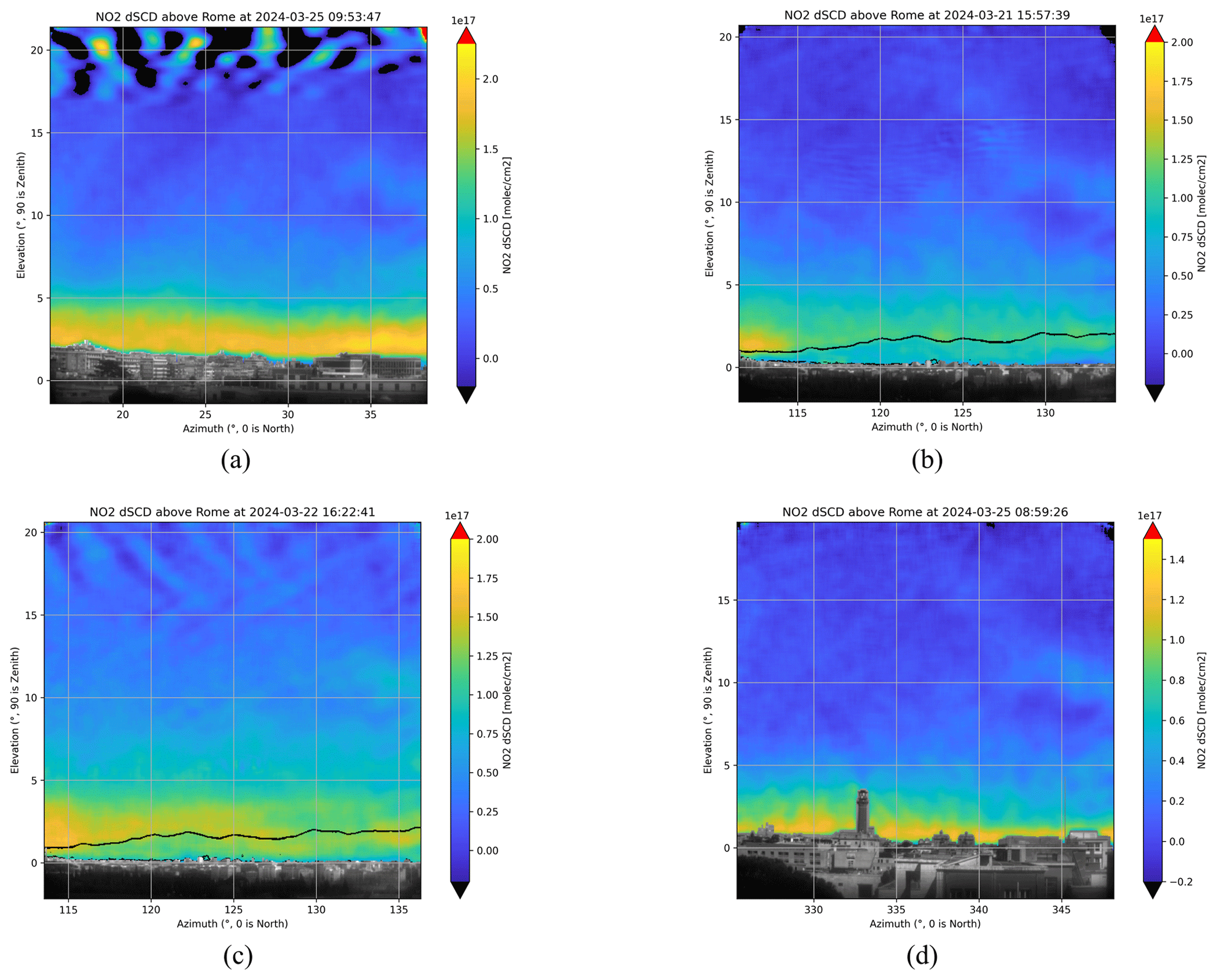
Figure 10 NO₂ dSCD maps for the four main azimuth directions in the measurement campaign. Note the different scales for the different directions. All times shown are UTC. On panels (a) and (c), the effects of moving clouds or aerosols are visible at the top of the image.

In addition to the quantitative comparison shown in Table 4, a qualitative comparison can also be made with the reference instruments. Figure 11 shows a NO₂ dSCD map taken in the direction of 124°, with overlays showing the corresponding MAX-DOAS and Pandora dSCDs. Similar patterns are found with all three measurement instruments.

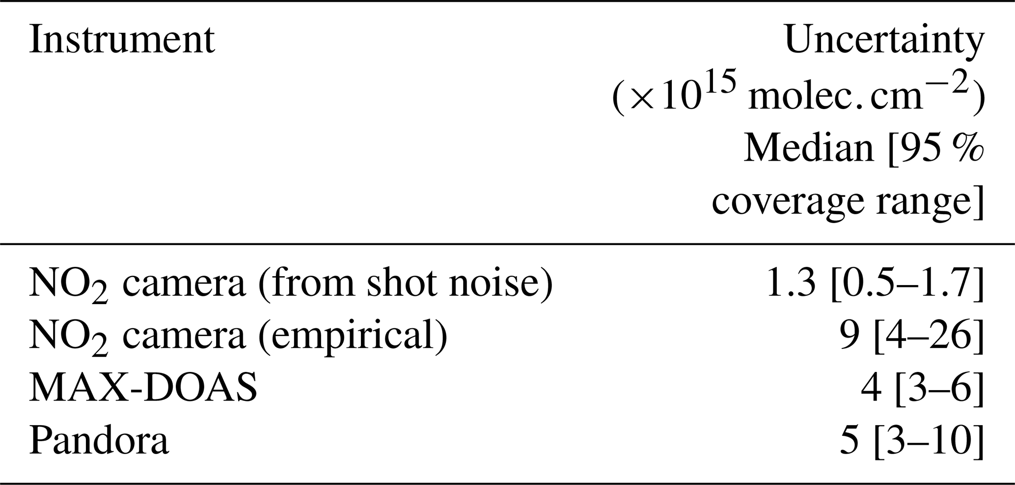
5.4 Uncertainties

Previous sections have already described the methodology followed by each instrument for uncertainty estimation. Table 5 presents summary statistics on the resulting estimated errors. As already mentioned, systematic or structured uncertainties are not (yet) considered for the NO₂ camera retrievals, so we expect serious underestimation of uncertainty. As a pragmatic alternative, we also report the standard deviation of NO₂ dSCDs among all pixels from the same elevation and same cube, which we consider to be an empirical estimate of retrieval errors. This probably overestimates the uncertainty, especially at low elevations, because it also includes the true azimuthal variation of the NO₂ field. On the other hand, the empirical indicator might underestimate the uncertainty in the case of a systematic bias. However, the comparison with the other instruments in Fig. 9 did not reveal any such bias, so we believe that this empirical approach is valuable.

6 Conclusions

We have presented the results of an intercomparison campaign between the NO₂ camera, an AOTF-based spectral imager optimized for the measurement of NO₂ slant column densities (SCDs) from the scattered solar light in the 425–455 nm domain, and two reference diffraction grating-based spectrometers: MAX-DOAS and Pandora. The three instruments were deployed in March 2024 at the BAQUNIN supersite on top of the physics department building of Sapienza University, located in the center of Rome, Italy. They were operated in such a way that the field of view of the NO₂ camera was sampled by the two other instruments at different azimuths and under strict coincidence criteria. The focus was on the NO₂ distribution close to the horizon, where local sources and winds are shaping the NO₂ field. Given the unconventional concept of the NO₂ camera, where wavelengths are acquired sequentially rather than simultaneously, the first and main purpose of the campaign was to validate its measured NO₂ SCDs with the coincident observations of the reference instruments. The secondary objectives were (1) to demonstrate that the NO₂ camera hyperspectral cubes can be processed by the DOAS method, the leading technique for the processing of UV–visible light spectra, and (2) to illustrate the capabilities of the NO₂ camera in revealing the spatial and temporal gradients of an urban NO₂ field.

The primary objective was achieved through the analysis of hundreds of coincident observations, which revealed that large NO₂ dSCDs ($>\mathrm{2}\times {\mathrm{10}}^{\mathrm{16}}\mathrm{molec}.{\mathrm{cm}}^{-\mathrm{2}}$) are usually well retrieved by the NO₂ camera. Those are typically found at low elevation angles, where the light crosses air masses of high NO₂ concentrations over long distances. Comparison of coincident observations with the MAX-DOAS and the Pandora instruments for elevations up to 10° shows good agreement (R²=0.86 for both), demonstrating that the NO₂ camera can provide meaningful quantitative information.

Table 5 Statistics on NO₂ dSCD uncertainty estimates for the whole campaign for each instrument, computed globally across all included elevation angles.

All of the camera acquisitions were performed in a “DOAS mode”, a driving scheme in which the AOTF bandpass filter is swept by small steps (0.15 nm) across a wavelength range in order to obtain continuous spectra. Contrary to diffraction grating-based instruments, regularly sampling a chunk of optical spectrum with fine steps requires excellent control of the AOTF. In general, no problem was found in applying the DOAS method, confirming the good tuning performance of the instrument. The main problems encountered were related to the stability of the shape of the AOTF response function and to changes in illumination conditions during the acquisitions, affecting the obtained NO₂ dSCDs.

While capturing spatial gradients is easy for a native imaging system such as the NO₂ camera, observations of extended scenes are not routinely performed by conventional operational air quality remote sensing instruments such as the MAX-DOAS and Pandora spectrometers. It requires the sequential pointing of the collecting optics in many pairs of azimuth and elevation angles. On the other hand, the light spectrum is captured at once. The images, eventually produced based on the results of the MAX-DOAS and Pandora measurements, lack details usually helpful for understanding the context of the observations or seeing fine-scale features. The 20°×20° field of view of the NO₂ camera could only be sampled by the other two instruments at the cost of long acquisition sequences. The variation of the temporal coincidence criteria, between ±5 and ±30 min, highlights the temporal variability of the urban NO₂ field, be it driven by changes in the emissions, light path or illumination conditions. In some scenes, local enhancements are clearly captured by the imager, revealing spatial gradients which would be hard to see with the other ground-based instruments.

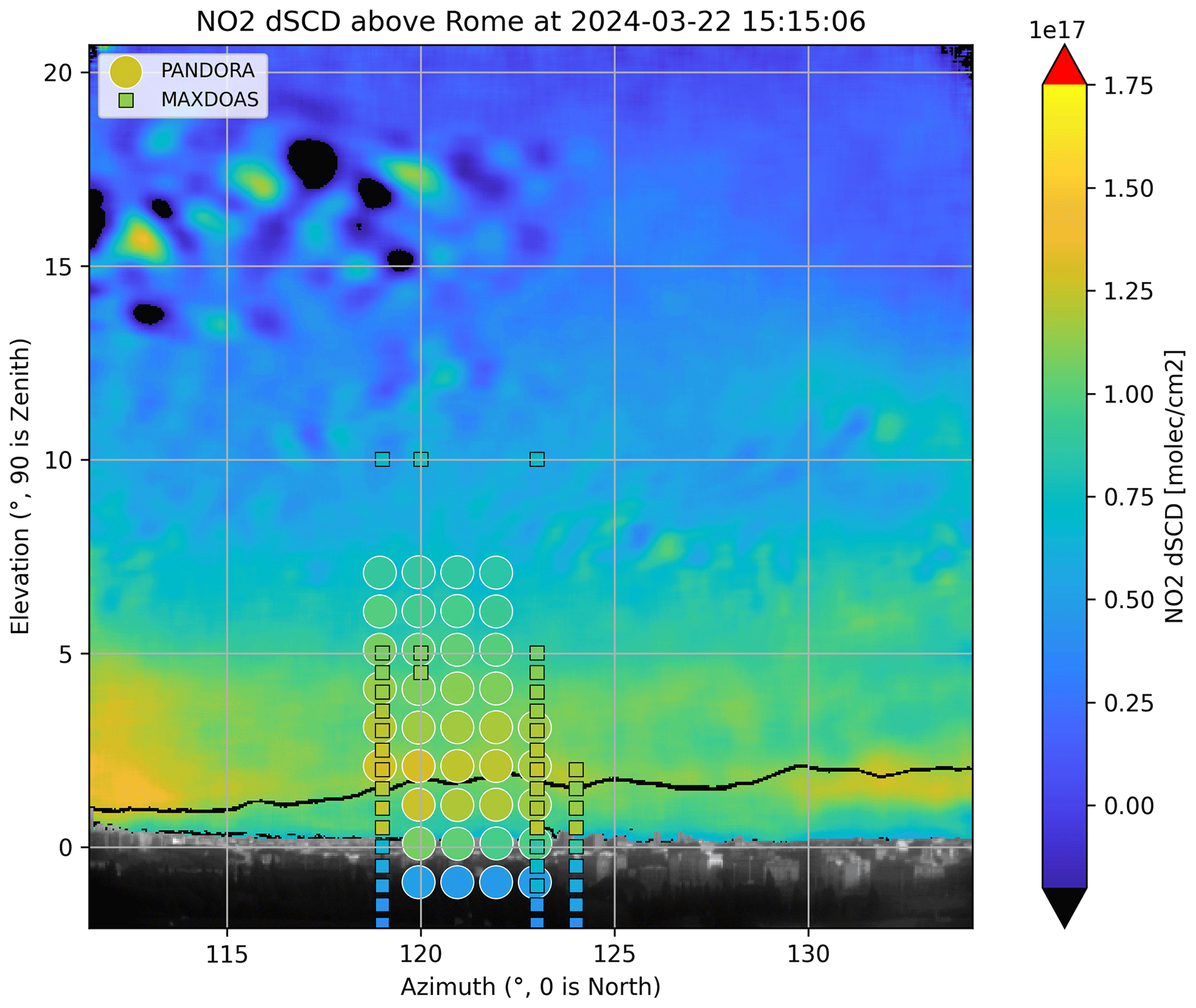
Figure 11 Qualitatively, the NO₂ dSCDs of both the Pandora and MAX-DOAS agree well with the dSCD obtained with the NO₂ camera. The size of the dots is not representative of the field of view of the instruments.

These encouraging results call for further usage of the NO₂ camera. First, the few local and transient enhancements that have already been detected are just a glimpse of the many more “pollution events” that can happen in an urban environment such as Rome. Long-term installation of the instrument as part of a supersite like BAQUNIN would allow for studying these events in order to understand their origin, their amplitude, their correlation with changes in the light path and the fate of the plume. Second, the tuning range of the instrument is not limited to 425–450 nm, such that the acquisition of spectral images in a region of strong O₄ absorption (470–480 nm) would allow for informing on the visual range of the pixel line of sight. This information will be required in order to retrieve tropospheric NO₂ columns from the NO₂ dSCD maps measured by the camera. Finally, the instrument itself can be improved further, mainly by increasing the frame rate of the detector, better characterizing the spectral response function and reducing the internal stray light.