Harmonisation of sixteen tropospheric ozone satellite data records

The first Tropospheric Ozone Assessment Report (TOAR, 2014–2019) encountered several observational challenges that limited the confidence in estimates of the burden, short-term variability, and long-term changes of ozone in the free troposphere. One of these challenges is the difficulty to interpret the consistency of satellite measurements obtained with different techniques from multiple sensors, leading to differences in spatiotemporal sampling, vertical smoothing, a-priori information, and uncertainty characterisation. This motivated the Committee on Earth Observation Satellites (CEOS) to initiate a coordinated activity VC-20-01 on improving the assessment and harmonisation of tropospheric ozone measured from space. Here, we report on work that contributes to this CEOS activity, as well as to the ongoing second TOAR assessment (TOAR-II, 2020–2025). Our objective is to harmonise the spatiotemporal perspective of (sixteen) satellite ozone data records, thereby accounting as much as possible for differences in vertical smoothing and sampling. Four harmonisation methods are presented to achieve this goal: two for ozone profiles obtained from nadir sounders (UV-visible, IR, and combined UV-IR), and two for tropospheric ozone column products derived by one of the residual methods (Convective Cloud Differential or Limb–Nadir Matching). We discuss to what extent harmonisation may affect assessments of the spatial distribution, seasonal cycle, and long-term changes in free tropospheric ozone, and we anchor the harmonised profile data to ozonesonde measurements recently homogenised as part of TOAR-II. We find that approaches that use global ozone fields as a transfer standard (here the Copernicus Atmosphere Monitoring Service ReAnalysis, CAMSRA) to constrain the harmonisation generally lead to the largest reduction of the inter-product dispersion (IPD) between satellite datasets. These harmonisation efforts, however, only partially account for the observed discrepancies between the satellite datasets, with a reduction of about 10 %–40 % of the IPD upon harmonisation, depending on the products involved and with strong spatiotemporal dependences. This work therefore provides evidence that it is not only the differences in spatiotemporal smoothing and sampling, but rather the differences in measurement uncertainty that pose the main challenge to the assessment of the spatial distribution and temporal evolution of free tropospheric ozone from satellite observations.

1 Introduction

Ozone plays a fundamental role in the Earth's atmosphere, and is deeply involved in several major environmental concerns, including air quality, climate change, and ultraviolet radiation. Ozone in the troposphere causes respiratory problems, reduces ecosystem productivity and acts as a greenhouse gas. More specifically, tropospheric ozone is the third most important anthropogenic contributor to greenhouse radiative forcing. The distribution of tropospheric ozone is highly variable over a wide range of spatial and temporal scales due to a complex interplay between dynamical, chemical, and radiative processes. Global monitoring systems are therefore faced with the great challenge of accurately capturing this variability at all scales of interest. This motivated the Committee on Earth Observation Satellites (CEOS) to initiate the coordinated activity VC-20-01 on improving the assessment and harmonisation of tropospheric ozone measured from space. Here, we present harmonisation methods developed within this CEOS activity and comprehensive analyses which contribute to the second phase of the Tropospheric Ozone Assessment Report (TOAR-II).

The first Tropospheric Ozone Assessment Report (TOAR) encountered several observational challenges that limited the confidence in estimates of the burden, short-term variability, and long-term changes of ozone in the free troposphere, especially when combining data records from multiple satellites with inherent differences in unit representation, vertical smoothing, a-priori information, uncertainty characterisation, and spatiotemporal sampling, including the definition of the tropospheric top level (Gaudel et al., 2018). Additional confounding factors are time-varying biases and the lack of harmonisation of geophysical quantities (including differences in units). All together, these factors reduce the confidence in the observed distributions and trends of tropospheric ozone, impeding firm assessments relevant for science and policy. In this work, contributing to TOAR-II, we therefore go beyond the more common harmonisation procedures involving spatiotemporal (re)sampling or bias correction schemes (Shi et al., 2024). Our objective is to harmonise the vertical perspective of different ozone data records from satellites in several ways, accounting as much as possible for their vertical smoothing and sampling differences. This is mainly achieved by applying tropospheric top level definition harmonisation, and a-priori information harmonisation on several types of tropospheric ozone products, described in Sect. 2. The inherent differences between these satellite data records, as outlined above, result in a multitude of technical harmonisation needs, which are detailed in Sect. 3 of this work.

A first class of products is obtained through an inversion of spectral measurements by nadir-viewing sounders into a vertical ozone profile. We illustrate several approaches to harmonise the differing profile retrievals by making use of their vertical averaging kernels and prior information. Building on the Complete Data Fusion framework (CDF, Ceccherini et al., 2022), the latter can be effectively removed or replaced by a common transfer standard, which in this work is taken from the Copernicus Atmosphere Monitoring Service Re-Analysis (CAMSRA, Inness et al., 2019). Two nadir profile harmonisation approaches are eventually assessed in detail in Sect. 4. A selection of satellite data records is intercompared before and after harmonisation, while monthly gridded ozonesonde reference data originating from the TOAR-II HEGIFTOM (Harmonisation and Evaluation of Ground-based Instruments for Free Tropospheric Ozone Measurements) Working Group serve as an anchoring point (Van Malderen et al., 2025). A second class of tropospheric ozone products is obtained through subtraction of the stratospheric component from space-based total column observations. We present and evaluate how these can be harmonised to a common tropospheric top level in Sect. 5, again using two different approaches and involving the CAMS reanalysis as a transfer standard. The last section before the conclusions, Sect. 6, reports on the effects of the presented harmonisation methods on tropospheric ozone assessments in terms of (zonal) mean distributions, seasonal cycles, and long-term trends, spanning 21 years in total (January 2003–December 2023). This approach provides a thorough view on how the discrepancies between the satellite data records and the tropospheric ozone assessments resulting therefrom change upon harmonisation.

2 Tropospheric ozone data records

We consider three types of remotely sounded tropospheric ozone data records, and one reanalysis that is used as a transfer standard for harmonisation between them, all listed in Table 1. A Level-3-like (monthly gridded) ozonesonde dataset allows anchoring the harmonised satellite data to ground-based reference data.

Table 1 Tropospheric ozone products considered in this work, with Level-2 and Level-3 (GOP-ECV only) nadir profile products, limb/reanalysis-nadir matching products, and convective cloud differential products, from top to bottom, respectively, separated by horizontal lines. The two last rows specify the CAMS reanalysis that serves as a transfer standard and the Level-3-like ozonesonde reference data, respectively. Note that the fourth column provides the sampling resolution of the products as input to this work, while the native sampling resolution of the instruments is usually higher.

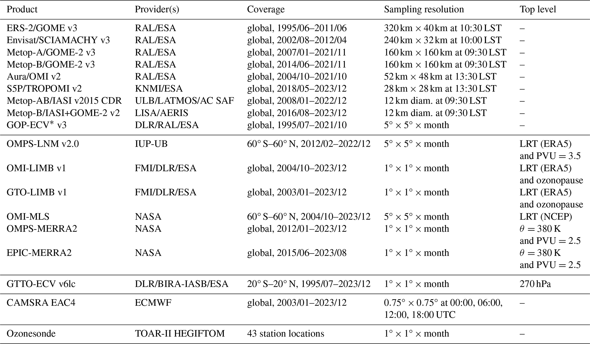
^* Although GOP-ECV provides full ozone profiles, we consider its lowest (surface to 450 hPa) subcolumn in this work only.

2.1 Nadir profile products

A first class of tropospheric ozone data records is provided by satellite instruments performing nadir-viewing irradiance observations. From each spectral observation, a vertically resolved ozone profile can be retrieved, indicated as Level-2 data. Monthly gridded averages are denoted as Level-3. Eight nadir ozone profile products from four independent Level-2 retrieval processors are considered, as listed in Table 1. Five of these originate from the Rutherford Appleton Laboratory (RAL) UV-visible processor versions 2 and 3, as developed within UK's National Centre for Earth Observation (NCEO) and ESA's Climate Change Initiative (CCI) on ozone (Miles et al., 2015). Next to that, the operational nadir ozone profile retrieval from TROPOMI (TROPOspheric Monitoring Instrument) is considered, also originating from UV-band observations (Keppens et al., 2024). The Infrared Atmospheric Sounding Interferometer (IASI) on both the Metop-A and Metop-B satellites operated by EUMETSAT yields vertically resolved day- and nighttime observations of atmospheric ozone (Hurtmans et al., 2012). Finally, the joint retrieval product developed at LISA (Laboratoire Inter-universitaire des Systèmes Atmosphériques) combines observations from the IASI and GOME-2 (second generation of the Global Ozone Monitoring Experiment) instruments onboard Metop-B at the native resolution of the former (Cuesta et al., 2013). To all Level-2 datasets, profile screening as recommended by the respective data providers has been applied. Additionally, we have limited all observations to solar zenith angles below 80°, which means that only daytime observations are considered for the infrared sounders, hence the mentioning of one overpass time in Table 1. Vertical smoothing harmonisation can be applied to these Level-2 datasets only if the data include initial prior profiles, averaging kernels and covariance matrices (see Sect. 4).

2.1.1 RAL UV-visible retrieval

The ERS-2 GOME (Global Ozone Monitoring Experiment, 1996–2011), Envisat SCIAMACHY (SCanning Imaging Absorption spectroMeter for Atmospheric CartograpHY, 2002–2012), Metop-A GOME-2 (2007–2021), Metop-B GOME-2 (2014–2023), and AURA OMI (Ozone Monitoring Instrument, 2004–2021) nadir ozone profile data were retrieved by the Rutherford Appleton Laboratory retrieval scheme; version 2 for OMI and version 3 for the other sensors. Each ozone profile is provided on a fixed vertical grid with 20 levels ranging between 0–80 km. The RAL retrieval is a three-step process (Miles et al., 2015). In the first step, the vertical profile of ozone is retrieved from Sun-normalised radiances in selected wavelength intervals of the ozone Hartley band, in the range 265–307 nm, which primarily contains information on stratospheric ozone. Prior ozone profiles come from the McPeters–Labow–Logan climatology (McPeters et al., 2007), except in the troposphere where a fixed value of 10¹² molecules cm⁻³ is assumed. A correlation length of 6 km is applied to construct the a-priori covariance matrix. In the second step, the surface albedo for each of the ground pixels is retrieved from the Sun-normalised radiance spectrum between 335–336 nm. Then, in step three, information on lower stratospheric and tropospheric ozone is added by exploiting the temperature dependence of the spectral structure in the ozone Huggins bands (323–335 nm). In this step, the a-priori ozone profile and its error are the output of step one, except that a prior correlation length of 8 km is imposed. RAL's radiative transfer model (RTM) is derived from GOMETRAN (Rozanov et al., 1997), but the original code has been modified substantially in order to increase its efficiency without losing accuracy. Within the RTM, there is no explicit representation of clouds, but their effects are incorporated as part an effective Lambertian surface albedo from step 2 of the retrieval. Therefore, a negative bias in retrieved ozone – proportional to the cloud-covered partial ozone column – is to be expected in the presence of high or optically thick clouds. The RAL L2 products have been validated by Keppens et al. (2018), and an OMI dataset of shorter duration from this scheme was one of the satellite products that contributed to TOAR (Gaudel et al., 2018).

2.1.2 TROPOMI operational data

TROPOMI is the unique payload on the Copernicus S5P satellite, the first atmospheric composition mission in the European Union Copernicus Earth Observation Programme (Ingmann et al., 2012). The field of view at nadir produces ground pixels of 5.5 km×3.5 km (along × across track) since the pixel size switch in August 2019, and of 7 km×3.5 km before. The large swath width of 2600 km produces a nearly daily coverage of the global (sunlit) atmosphere, with narrow gaps between orbits at the Equator. The operational TROPOMI ozone profile algorithm developed at KNMI derives the ozone concentration as a number density at 33 pressure levels throughout the atmosphere (surface to roughly 80 km) from the TROPOMI reflectance observations in the wavelength region between 270–330 nm, provided by Bands 1 (267–300 nm) and 2 (300–332 nm) of the UV detector. The main elements of the retrieval algorithm are the forward model and the Optimal Estimation (OE) fitting (Rodgers, 2000). Before the OE algorithm, several pre-processing steps are applied to the measured spectra. The operational TROPOMI ozone profile retrieval algorithm is discussed and validated with respect to ozonesonde and lidar observations in Keppens et al. (2024).

2.1.3 FORLI-O3 retrieval for IASI

The Metop-A and Metop-B IASI nadir ozone profile data for 2008–2019 and 2019–2022, respectively, were generated using the FORLI-O3 (Fast Optimal Retrievals on Layers for IASI Ozone) version 20151001 (Hurtmans et al., 2012). FORLI-O3 relies on a fast radiative transfer and a retrieval algorithm based on the OE method (Rodgers, 2000). Ozone is retrieved using the 1025–1075 cm⁻¹ spectral range, which is dominated by ozone absorption. The a-priori information used in the FORLI-O3 algorithm consists of a single global ozone prior profile, although the prior covariance matrix is built from the McPeters–Labow–Logan climatology (McPeters et al., 2007), as for RAL. The FORLI-O3 product consists of a vertical profile retrieved on a uniform and fixed 1 km vertical grid on 40 layers from the surface up to 40 km, with an extra residual layer from 40 km to the top of the atmosphere (60 km in practice). At nadir, the profiles have a 12 km diameter circular footprint, which stretches to an ellipsoid off-nadir. For this work, the Climate Data Record (CDR, v2024) reprocessing of the data at EUMETSAT AC SAF (Satellite Application Facility on Atmospheric Composition Monitoring, product O3M-521.1) is considered, meaning that consistent time series were used for the auxiliary data (Boynard et al., 2025). Therefore, a single data record combining the IASI-A and IASI-B data, with switch on January first, 2019, is used.

2.1.4 IASI+GOME-2 joint retrieval

Multispectral observations of ozone profiles from the synergism of IASI thermal infrared and GOME-2 ultraviolet measurements have been developed by Cuesta et al. (2013) at LISA, in collaboration with the Harvard–Smithonian Center for Astrophysics (USA), the Karlsruhe Institut für Technologie (Germany), and the Chinese Acadamy of Sciences (China). With both instruments on board the Metop satellite series, this multispectral satellite approach is designed for observing the vertical profile of ozone with enhanced sensitivity, particularly in the lowermost troposphere, as compared to single-band approaches. It offers a relatively fine ground resolution: 12 km diameter pixels spaced by 25 km at nadir, matching the IASI resolution. The IASI+GOME-2 observations considered here are obtained from morning overpasses of the Metop-B satellite and for low cloud-fraction scenes (GOME-2 pixels with cloud fractions below 30 %). The resulting product is provided as vertical profiles of ozone on the same fixed altitude grid as the IASI products (see above). Validation against ozonesondes shows low mean biases (below 3 %), an average precision of 16 %, and a correlation coefficient of 0.86 for the lowermost tropospheric ozone retrievals (Tarasick et al., 2019).

2.1.5 DLR UV-visible merge

Finally, one additional Level-3 merged nadir ozone profile product is considered. The GOME-type Ozone Profile Essential Climate Variable (GOP-ECV, version 3, Coldewey-Egbers et al., 2025) data record has been developed in the framework of the European Space Agency's Climate Change Initiative on ozone (ESA Ozone_cci+). It combines bias-corrected ozone profile measurements from five nadir-viewing ultraviolet-visible-near-infrared (UVN) satellite sensors including GOME/ERS-2 (1995–2011), SCIAMACHY/Envisat (2002–2012), OMI/Aura (2004–today), GOME-2/MetOp-A (2007–2021), and GOME-2/MetOp-B (2013–today). The height-resolved ozone profiles are retrieved using the RAL scheme that is applied to all sensors. For GOP-ECV, the derived partial columns for 19 layers from the surface to 80 km are utilised. In a first step, the profiles from the individual sensors are merged into a single record based on deseasonalised anomalies. Data from OMI is used as a reference and observations from the other sensors are adjusted to that reference based on comparisons during overlap periods. At least six years of overlap with OMI is available for all sensors. In a second step, the merged profiles are scaled in order to match the integrated columns from the profiles with the total ozone columns from the corresponding GTO-ECV (GOME-type Total Ozone Essential Climate Variable) data record (Coldewey-Egbers et al., 2022, and references therein). The main objective of this procedure is to improve the long-term stability of the merged profile record by taking advantage of the excellent quality of GTO-ECV (Garane et al., 2018). The GOP-ECV product provides monthly mean ozone profiles at a spatial resolution of 5°×5° from July 1995 through October 2021. For this study only the partial ozone columns from the lowermost profile layer (surface to 450 hPa) are used.

2.2 Combination of nadir and limb/reanalyses data

The limb/reanalysis-nadir matching tropospheric ozone column products are created by subtracting a stratospheric ozone column from a spatiotemporally matching nadir total ozone column observation, whereby the stratospheric profile can be obtained from either limb sounding or reanalysis data. In this work, we consider the scientific limb-nadir matching (LNM) tropospheric ozone product developed at Bremen University (IUP-UB), two LNM products created at the Finnish Meteorological Institute (FMI), and three NASA products, of which two use MERRA2 (Modern-Era Retrospective analysis for Research and Applications version 2) as reanalysis for the stratospheric column.

2.2.1 IUP product

The Ozone Mapping and Profiler Suite (OMPS) LNM product is generated by combining the retrieved total ozone columns from the OMPS Nadir Mapper (OMPS-NM) with limb profiles from the OMPS Limb Profiler (OMPS-LP). A stratospheric ozone column is calculated from OMPS-LP ozone profile retrievals and subtracted from the total ozone column retrieved from OMPS-NM using the weighting function fitting approach (Orfanoz-Cheuquelaf et al., 2024). The latter is done only for those across-track pixels that are co-located to the location of the tangent point of the limb ozone profiles, which is usually around the centre of the swath. Both retrievals are completely independent of each other, yet, for consistency, they use the same ozone absorption cross-sections. For the data up to 2018, it has been found that this product overall seems biased low by a few DU, but its seasonality and inter-annual variability are in good agreement with all comparison datasets (Orfanoz-Cheuquelaf et al., 2024). In this work, all available data ranging from 2012 to 2022 are considered.

2.2.2 FMI products

Within FMI's LNM products, OMI or GTO (GOME-type Total ozone) are used for the total ozone column data. For OMI, clear-sky total ozone column data are processed with the GODFIT v4.0 algorithm (Lerot et al., 2014). The other source of total column is the daily mean total ozone from the GTO dataset, which provides data in both cloudy and cloud-free conditions (Coldewey-Egbers et al., 2022). The stratospheric ozone column is derived from a combination of ozone profiles from several satellite instruments in limb-viewing geometry, as described in Sofieva et al. (2022). The stratospheric ozone column is computed either from the tropopause or from 3 km below the thermal tropopause. The stratospheric columns are subtracted from the clear-sky measurements by the nadir sensors, daily. The daily values are averaged to monthly mean values subsequently. The horizontal resolution of OMI-LIMB and GTO-LIMB tropospheric ozone column is 1°×1°, and the dataset covers the period 2004–2023. A more detailed description of the retrievals can be found in Sofieva et al. (2022).

2.2.3 NASA products

Finally, several satellite-derived tropospheric ozone column products are made available by NASA's Goddard Space Flight Center (GSFC). These include TOMS (Total Ozone Mapping Spectrometer) monthly columns (1979–2005, not considered in this work), OMI-MLS (OMI total ozone minus Microwave Limb Sounder stratospheric ozone) monthly columns (2004–2023), EPIC-MERRA2 (Earth Polychromatic Imaging Camera total ozone minus MERRA2 stratospheric ozone) monthly columns (2015–2023), and OMPS-MERRA2 daily columns (2012–2023). These datasets all represent gridded monthly-mean or daily-mean tropospheric ozone columns in Dobson Units, determined by subtracting co-located daily stratospheric column ozone from daily total column ozone, optionally followed by monthly averaging. For the OMI-MLS product, the daily stratospheric column ozone is obtained from the MLS, which is two-dimensionally interpolated to fill in between MLS orbital gaps (Ziemke et al., 2006). Note that the OMI total ozone column product used here is based on the Collection 3 level-1b data, which in the meantime has been replaced by Collection 4 (Kleipool et al., 2022), but the latter has not yet been thoroughly evaluated. For EPIC and OMPS nadir-mapper products, the stratospheric ozone column is determined from MERRA2 analyses that assimilate MLS ozone. As tropospheric top level, the EPIC and OMPS Nadir Mapper products use the MERRA2 PV-theta (2.5 PVU, 380 K) tropopause pressure while OMI/MLS uses the NCEP reanalyses lapse-rate tropopause (LRT) pressure (also see details in Table 1).

2.3 Convective cloud differential products

The Convective Cloud Differential (CCD) method obtains tropospheric ozone columns by subtracting above-cloud total ozone column observations from clear-sky observations by the same instrument, and is therefore self-calibrating. The GOME-type Tropical Tropospheric Ozone Essential Cimate Variable (GTTO-ECV) generated within ESA's Climate Change Initiative programme is a tropospheric ozone Climate Data Record ranging 1995 to end of 2023 (Heue et al., 2016). GTTO-ECV combines data from GOME, SCIAMACHY, OMI, the three GOME-2 missions, and TROPOMI. The mean bias as well as the mean annual cycle relative to the reference instrument (OMI) are used to correct for the differences between the seven input sensors. The tropospheric ozone column retrieval based on the CCD technique limits the product's coverage to the tropical belt (20° S–20° N). Two monthly mean datasets at 1°×1° resolution are generated: one corresponds to a tropospheric column up to 200 hPa as in the first CCI data release (Heue et al., 2016), while the other is limited to 270 hPa, as this pressure level is also used in the operational TROPOMI dataset. Only the latter dataset is considered in this work.

2.4 CAMS transfer standard

The global model field that is used as a transfer standard for the satellite data harmonisation in this work is the CAMS reanalysis EAC4 (CAMSRA, Inness et al., 2019) produced by the Copernicus Atmosphere Monitoring Service (CAMS, Peuch et al., 2022) that is operated by ECMWF on behalf of the European Commission. EAC4 consists of three-dimensional time-consistent atmospheric composition fields, including aerosols and chemical species. The CAMS reanalysis was produced using 4D-Var data assimilation in Cycle 42r1 of ECMWF's Integrated Forecasting System (IFS), assimilating satellite retrievals of total column CO, tropospheric column NO₂, aerosol optical depth, and ozone columns and profiles in addition to meteorological observations. Although the assimilated ozone data does not involve any of the retrieval products discussed in this work, it should be noted that some of the assimilated total ozone column data originates from the same instruments. It is here assumed that this results in negligible data correlations only, as column and profile retrievals originate from different parts of the observed spectra. EAC4 has 60 vertical model levels between the surface and 0.1 hPa and a horizontal resolution of about 80 km. Six-hourly, three-dimensional analysis and forecast fields, as well as hourly surface forecast fields, are available form CAMS's Atmosphere Data Store (ADS). On the ADS, the fields are interpolated from their native representation to a regular 0.75°×0.75° latitude-longitude grid. For this work, we interpolate the multiple daily CAMSRA UTC fields to monthly mean local solar time (LST, noon or satellite overpass time) within one-degree boxes for our harmonisation purposes.

Offline or reprocessed data were assimilated in EAC4 between 2003–2016 and near-real time (NRT) data from 2017 when the reanalysis production was running close to NRT. Such changes in the observing system, e.g. the end of SBUV/2 (Solar Backscatter Ultraviolet Radiometer-2) data and the introduction of ozone retrievals from TROPOMI, OMPS and Metop-C GOME-2 at the beginning of 2021, affect the quality of the ozone analysis field and lead to changes in the tropospheric ozone bias (Inness et al., 2019). The EAC4 validation reports (available from https://atmosphere.copernicus.eu/eqa-reports-global-services, last access: 17 November 2025) show that around 2018 a positive bias in ozone starts to develop around the tropopause according to comparisons against ozonesondes, and is also seen in the comparison with IASI ozone retrievals. For tropospheric ozone, there are indications of improvements in Northern Hemisphere mid-latitudes since 2021, but also of somewhat increased biases in other regions. Increased ozone biases are also seen in some of the earlier years, i.e. between March–August 2004 when no ozone profile data were available for assimilation. This affects the vertical structure of the ozone analysis and leads to larger biases with respect to ozonesondes, especially in the Antarctic. From 2013 onwards, there is a larger seasonally varying bias in ozone in the free troposphere, particularly in the Arctic and Antarctic. The reason for this bias is a change in the observing system, namely the change from 13-layer SBUV/2 data to 21-layer SBUV/2 data in July 2013 that unfortunately had an impact on tropospheric ozone. The effect of these assimilation data (quality) changes on the reanalysis can be expected to be of the same order as the effect of choosing between a full reanalysis and a yearly climatology that is derived therefrom, as discussed next.

In this work, we have opted for the full CAMS reanalysis as a transfer standard, instead of using a yearly climatology that does not capture long-term temporal tropospheric ozone (column) changes. Although this choice comes with the risk of introducing a tropospheric ozone trend component from the CAMS reanalysis in the harmonised data that is not in the initial satellite data, it is assumed to provide a better representation of the actual tropospheric (ozone) dynamics (i.e. the risk of removing actual dynamics using the climatology is larger). Figure 1 provides an indication of the maximal effect of this choice on the CAMSRA harmonisation terms that correct tropospheric ozone columns for their different tropospheric top levels. It shows the difference between the correction terms for a derived climatology (ranging August 2004–December 2016, i.e. only reprocessed data including MLS) and the full reanalysis, upon going from a 450 hPa top level tropospheric column to a lapse-rate tropopause column (two common definitions with maximum vertical separation). Vertical lines indicate changes in the CAMS assimilation system as described above and detailed in Inness et al. (2019). Despite differences up to 2 DU towards the beginning and the end of the time series, the choice between the use of a climatology or the full reanalysis usually results in less than 1 DU (3 %–4 %) differences in the harmonised products.

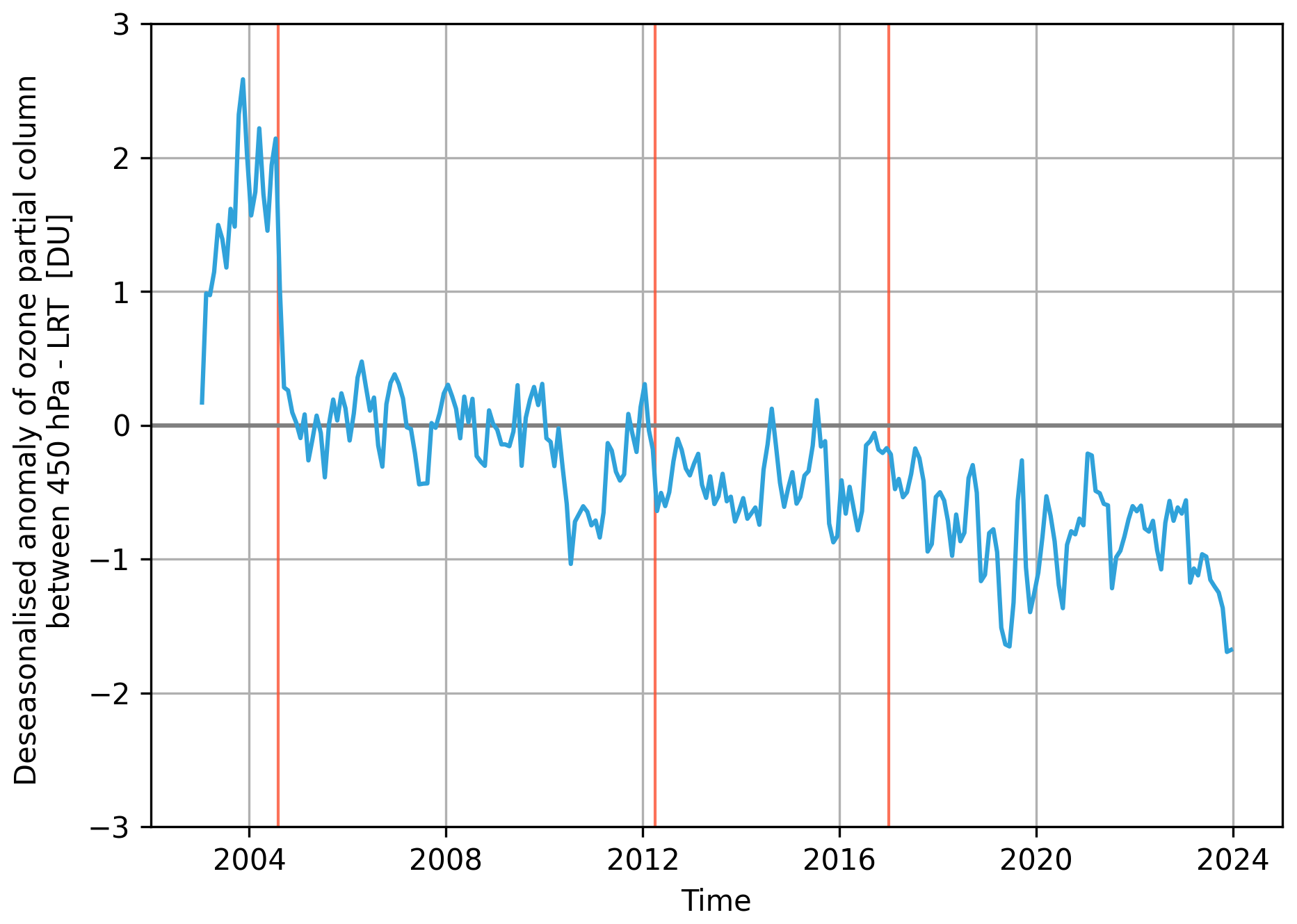
Figure 1 Difference (blue) between the derived climatology (2004–2016) and full reanalysis CAMS correction terms for going from the 450 hPa top level tropospheric column to the lapse-rate tropopause column. Vertical lines (red) indicate important changes in the CAMS assimilation system as detailed in Inness et al. (2019).

2.5 Ozonesonde reference data

The ozonesonde is a small and lightweight instrument that measures atmospheric ozone concentrations by pumping and bubbling air in differing concentrations of potassium iodide (KI) solutions in electrochemical concentration cells (ECC, Tarasick et al., 2021). Being coupled with a radiosonde during a weather balloon flight, it provides vertical ozone profiles up to about 30–35 km altitude with a stated precision of 3 %–5 % and a total uncertainty of about 5 %–10 %, for both the troposphere and stratosphere (Smit et al., 2021). A major contributor to uncertainties in ozone trends are discontinuities and biases in the long-term records of ozonesonde sites. Therefore, an Ozonesonde Data Quality Assessment (O3S-DQA) was initiated in 2011 to homogenise temporal and spatial ozonesonde data records under the framework of the SI2N initiative on “Past Changes in the Vertical Distribution of Ozone” (Hassler et al., 2014). The O3S-DQA homogenisation serves three major needs: (i) remove all known inhomogeneities or biases due to changes in equipment, operating procedures or processing, (ii) strengthen the consistency within the ozonesonde network by providing and applying standard guidelines for data (re)processing steps (Smit et al., 2021), and (iii) provide an uncertainty estimate for each ozone partial pressure measurement in the profile.

Within the HEGIFTOM (Harmonisation and Evaluation of Ground-based Instruments for Free Tropospheric Ozone Measurements) working group of the TOAR-II initiative, the homogenised O3S-DQA data from 43 ozonesonde stations has been processed into L3-like monthly gridded tropospheric ozone products (Van Malderen et al., 2025). More specifically, monthly mean tropospheric ozone columns are calculated for three definitions of the top of troposphere (see next section), if at least two ozonesonde profiles are available within that month. The related monthly mean uncertainties are given by the square root of the sum of the (squared) measurement uncertainties of the individual profiles and the statistical uncertainty; clearly, the statistical uncertainty is by far the dominant contribution here, although the uncertainty of each tropospheric ozone column is just obtained by summing up the individual (random) uncertainties at the different pressure levels and therefore constitutes an overestimation of the true uncertainty. The monthly tropospheric ozone column data from all 43 ozonesonde stations are collected into monthly gridded data structures. For the one-degree grid selected in this work, this results in having one station per grid cell at maximum, with 0.066 % ($\mathrm{43}/\mathrm{64}\mathrm{800}$) of the global grid cells being covered. The ozonesonde station density, however, is higher over Europe, North-America, and the Antarctic, where hence the comparative analysis for this work is focused.

3 Harmonisation needs

Given the inherent differences between tropospheric ozone products from satellites, inducing substantial challenges for tropospheric assessments (see Introduction), in this work we aim at the following harmonisation approaches:

• Account for different vertical representations. Ozone concentration values in volume mixing ratio on pressure levels are vertically integrated to Dobson Units (DU) over a predefined pressure range (see next item). If needed, unit conversions are performed using auxiliary data that are provided in the ozone data files (Keppens et al., 2019).

• Account for different tropospheric top levels. The pressure range for vertical integration goes from the surface to three top level definitions: (a) 450 hPa globally, (b) four latitude-dependent pressure levels (150 hPa in the tropics (<15°), 200 hPa in the subtropics (15–30°), 300 hPa at mid-latitudes (30–60°), and 400 hPa in the polar regions (>60°)), and (c) the thermal tropopause obtained from MERRA2 temperature fields using the WMO lapse rate definition (Hoffmann and Spang, 2022; Zou et al., 2023). The latter two definitions serve as guidelines for the TOAR-II community (https://igacproject.org/sites/default/files/2022-03/TOAR-II_Guidelines_for_TCO_and_Profile_Intercomparisons.pdf, last access: 30 November 2024). Differences between the satellite data top levels and these definitions can be accounted for in several ways, including the use of the CAMSRA transfer standard interpolated to the satellite observation coordinates, see Sect. 5.

• Account for different surface pressures. Vertical harmonisation operations are performed on the given satellite pressure grid, but vertical integration to obtain tropospheric columns from profiles is performed from the CAMSRA surface pressure to the common top level definition (previous item).

• Account for different spatial sampling. Horizontal (re)sampling into 1°×1° boxes, if needed, with their centres ranging from −89.5 to 89.5° in latitude, and from −179.5 to 179.5° in longitude. Comparisons are moreover limited to those grid cells that have data for all satellite instruments involved. Products with 5°×5° horizontal resolution are not interpolated though.

• Account for different temporal sampling. Temporal (re)sampling into monthly bins.

• Account for different a-priori information sources. Having the CAMSRA transfer standard as a common source for the a-priori ozone profile for the nadir profile retrievals. This means the prior information in each retrieved profile has to be replaced by the corresponding (by horizontal interpolation) CAMSRA profile. Additionally, the CAMSRA data with UTC time stamps are temporally interpolated to noon local solar time for each longitude, in order to have a realistic common reference for all daytime satellite overpass times.

• Account for different a-priori information contributions. Optimally estimated nadir ozone profiles, which typically have a vertical sensitivity below one in the troposphere meaning that part of the retrieved information originates from prior constraints, are converted to an effective unit-sensitivity representation.

These harmonisation practices are all applied simultaneously, except for the last two, where one has to choose either one or the other. There is no use in applying profile prior replacement and prior contribution correction at the same time, see Sect. 4 for details.

4 Profile harmonisation

4.1 Methods

Nadir sounding of an atmospheric ozone profile typically involves an under-constrained retrieval process. Such a process includes a forward model inversion and a cost function minimisation, whereby the latter must be converted from an under-constrained problem to a constrained one using external information (Rodgers, 2000). The constraining information can either consist of an a-priori estimate of the atmospheric state and its covariance, like in the Optimal Estimation (OE) approach, or of a continuity constraint, like in Philips–Tikhonov-like approaches. In both cases, the resulting retrieved state unavoidably consists of a mixture of measurement information and prior constraints. The presence of prior information in atmospheric state retrievals however complicates their scientific application and interpretation in several ways (von Clarmann and Grabowski, 2007). In comparisons with other measured or modelled data, differences and their uncertainties contain several prior-induced terms that can be hard to assess: It is virtually impossible to tell whether significant structures originate from the measurement or from the a-priori, as was the case for the first Tropospheric Ozone Assessment Report (Gaudel et al., 2018). On the other hand, the use of an a-priori distribution with much simpler spatiotemporal structure and loose(r) prior covariance enables distinctions to be made between structures in the prior, retrieved, and correlative information. Further, depending on the nature of the prior information, profile retrievals at different locations are no longer statistically independent, which complicates their averaging and assimilation (Ceccherini et al., 2014; von Clarmann and Glatthor, 2019). It is therefore desirable to harmonise the a-priori information between retrieved products upon their combined assessment, or even to remove it entirely (if possible).

Optimal estimation retrievals have the advantage that their information mixing is fully quantified by the retrieval's averaging kernels (Rodgers, 2000), represented by a single vector kernel for column retrievals, or by a square averaging kernel matrix for vertically resolved profile retrievals. Consequently, it is in principle possible to perform a deconvolution operation that removes the prior information from the retrieval, resulting in a so-called information-centred representation of the retrieved atmospheric state, where each data point represents one independent degree of freedom (von Clarmann and Grabowski, 2007; Migliorini et al., 2008; Keppens et al., 2019, 2022). In practice, however, a pure deconvolution is hampered by the presence of the retrieval uncertainty as expressed by its covariance (matrix) and by the instability of the averaging kernel matrix inversion. Keppens et al. (2022) have demonstrated that, as a result, the information-centred representation is not suitable, i.e. within acceptable uncertainty, for monthly zonal mean assessments of the tropospheric ozone column (representing roughly one degree of freedom) from nadir ozone profile retrievals.

In order to reduce the differences between the retrieved ozone profile products that result from their different prior information, one must thus opt for prior information harmonisation instead of removal. This can be achieved using the complete data fusion (CDF) framework, although it was initially developed as a method for combining retrieved atmospheric states that is equivalent to their simultaneous retrieval (Ceccherini et al., 2015) and to their measurement space solution data fusion (Ceccherini, 2016). It has the ability to combine the (spatiotemporal fusion and) replacement of prior information with a vertical interpolation and a corresponding uncertainty assessment (Ceccherini et al., 2018). Based on the independent development of an alternative data fusion approach, involving the application of a Kalman filter (Schneider et al., 2022), the CDF formulation has recently been improved, now being valid also when the covariance matrices of the input products are singular (Ceccherini et al., 2022). In the latter reference, it has moreover been shown that both methods are mathematically equivalent. The latest formulation of the CDF framework has therefore been applied in this work for the prior information harmonisation between the selected ozone profile products, using CAMSRA as the joint new prior source. For an overview of other satellite data fusion approaches, e.g. see Xia et al. (2023).

Ceccherini et al. (2022) determine a profile ${\mathit{x}}_N^{\prime }$ as a complete data fusion of N profiles x_i, with corresponding covariance matrices S_i, averaging kernels A_i, and a-priori profiles x_a,i, as follows:

$$\begin{array}{}\text{(1)}& \begin{array}{rl}{\mathit{x}}_N^{\prime }& ={\left(\sum _{i=\mathrm{1}}^N{\mathbf{S}}_i^{-\mathrm{1}}{\mathbf{A}}_i+{{\mathbf{S}}_{\mathrm{a}}^{\prime }}^{-\mathrm{1}}\right)}^{-\mathrm{1}}\\ & \times \left(\sum _{i=\mathrm{1}}^N{\mathbf{S}}_i^{-\mathrm{1}}\left[{\mathit{x}}_i-(\mathbf{I}-{\mathbf{A}}_i){\mathit{x}}_{\mathrm{a},i}\right]+{{\mathbf{S}}_{\mathrm{a}}^{\prime }}^{-\mathrm{1}}{\mathit{x}}_{\mathrm{a}}^{\prime }\right)\end{array}\end{array}$$

where the sum is taken over the N profiles within a predefined spatiotemporal domain (monthly one-degree boxes in this work). I is the unit matrix having the same size as A_i, while ${\mathit{x}}_{\mathrm{a}}^{\prime }$ and ${\mathbf{S}}_{\mathrm{a}}^{\prime }$ are a new a-priori profile and covariance matrix that reconstrain the fused profile. It is hence clear that the CDF result is highly influenced by the choice of this new prior information, see below. The averaging kernel matrix and covariance matrix corresponding to ${\mathit{x}}_N^{\prime }$ are given by:

$$\begin{array}{}\text{(2)}& {\mathbf{A}}_N^{\prime }={\left(\sum _{i=\mathrm{1}}^N{\mathbf{S}}_i^{-\mathrm{1}}{\mathbf{A}}_i+{{\mathbf{S}}_{\mathrm{a}}^{\prime }}^{-\mathrm{1}}\right)}^{-\mathrm{1}}\left(\sum _{i=\mathrm{1}}^N{\mathbf{S}}_i^{-\mathrm{1}}{\mathbf{A}}_i\right)\end{array}$$

and

$$\begin{array}{}\text{(3)}& {\mathbf{S}}_N^{\prime }={\left(\sum _{i=\mathrm{1}}^N{\mathbf{S}}_i^{-\mathrm{1}}{\mathbf{A}}_i+{{\mathbf{S}}_{\mathrm{a}}^{\prime }}^{-\mathrm{1}}\right)}^{-\mathrm{1}}\end{array}$$

respectively. The fused profile and averaging kernel thus have the fused covariance matrix as a preceding scaling factor. Three typical choices for the new prior profile ${\mathit{x}}_{\mathrm{a}}^{\prime }$ (0, initial x_a, or new (model) x_m) and for the new prior constraint ${{\mathbf{S}}_{\mathrm{a}}^{\prime }}^{-\mathrm{1}}$ (0, initial ${\mathbf{S}}_{\mathrm{a}}^{-\mathrm{1}}$, or new (model) ${\mathbf{S}}_{\mathrm{m}}^{-\mathrm{1}}$) result in nine possible combinations of both, but not all of these are of scientific interest: A zero prior profile will just shift the retrieved profile to zero if the prior constraint (as the inverse of the prior covariance) is not set to zero as well. Besides, there is little use in harmonising the prior constraint if the prior profile is not harmonised at the same time. As such, five combinations of ${\mathit{x}}_{\mathrm{a}}^{\prime }$ and ${{\mathbf{S}}_{\mathrm{a}}^{\prime }}^{-\mathrm{1}}$ remain, but obviously other choices can be made. Note that a retrieval's x_i and S_i could in principle be considered for replacing the prior profile and covariance, but these would mimic a (next) retrieval iteration step and under-constrain the CDF, respectively.

The CDF framework is fully exploited by taking both the new prior profile and the new prior constraint from a retrieval-independent model (CAMSRA in this work), see Tables 2 and 3 (first row). If, on the other hand, one maintains the initial retrieval constraints, having ${{\mathbf{S}}_{\mathrm{a}}^{\prime }}^{-\mathrm{1}}=\sum {\mathbf{S}}_{\mathrm{a},i}^{-\mathrm{1}}=\sum {\mathbf{S}}_i^{-\mathrm{1}}(\mathbf{I}-{\mathbf{A}}_i)$, the direct a-priori profile replacement (APR, second row), from Rodgers and Connor (2003), Eq. (10), or Keppens et al. (2019), Eq. (16), is obtained. For a single retrieved profile, this conversion becomes very intuitive:

$$\begin{array}{}\text{(4)}& {\mathit{x}}_{\text{APR}}^{\prime }=\mathit{x}-(\mathbf{I}-\mathbf{A})({\mathit{x}}_{\mathrm{a}}-{\mathit{x}}_{\mathrm{m}})\end{array}$$

It is moreover identical to correcting the retrieved profile x for the averaging kernel-smoothed model profile:

$$\begin{array}{}\text{(5)}& {\mathit{x}}_{\text{APR}}^{\prime }=\mathit{x}+{\mathit{x}}_{\mathrm{m}}-\left[\mathbf{A}{\mathit{x}}_{\mathrm{m}}+(\mathbf{I}-\mathbf{A}){\mathit{x}}_{\mathrm{a}}\right]\end{array}$$

with the averaging kernel smoothing operation applied to x_m between square brackets (Keppens et al., 2019, Eq. 20). In the APR method, however, the resulting atmospheric state profile ${\mathit{x}}_{\text{APR}}^{\prime }$ will no longer represent an optimally estimated retrieval with respect to the new prior profile x_m, whereas this is indeed the case for the full CDF by construction. Taking the new prior profile and constraint to be identical to (the sum of) their initial value(s), the CDF method results in a mere weighted average (WAV) profile with corresponding kernels and covariances, see Tables 2 and 3 (third row).

Table 2 Approaches for harmonising ozone profile observations that include averaging kernels and covariance matrices, based on the general CDF method (first row). Harmonised profiles ${\mathit{x}}_N^{\prime }$ are obtained from N input profiles and determined by the choice for the new a-priori profile ${\mathit{x}}_{\mathrm{a}}^{\prime }$ and constraint ${{\mathbf{S}}_{\mathrm{a}}^{\prime }}^{-\mathrm{1}}$.

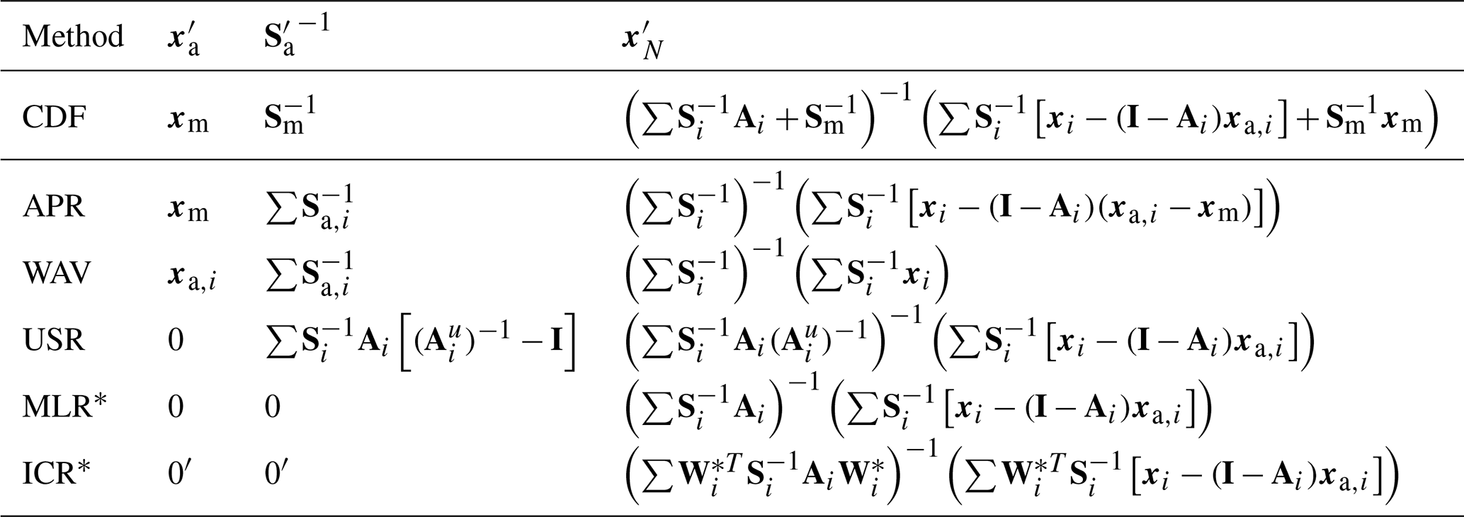
^* Not applied in this work.

Table 3 Approaches for harmonising ozone profile observations that include averaging kernels and covariance matrices, based on the general CDF method (first row). The averaging kernel matrices ${\mathbf{A}}_N^{\prime }$ and covariance matrices ${\mathbf{S}}_N^{\prime }$ that correspond to the harmonised profiles ${\mathit{x}}_N^{\prime }$ are obtained from N input profiles and determined by the choice for the new a-priori profile ${\mathit{x}}_{\mathrm{a}}^{\prime }$ and constraint ${{\mathbf{S}}_{\mathrm{a}}^{\prime }}^{-\mathrm{1}}$.

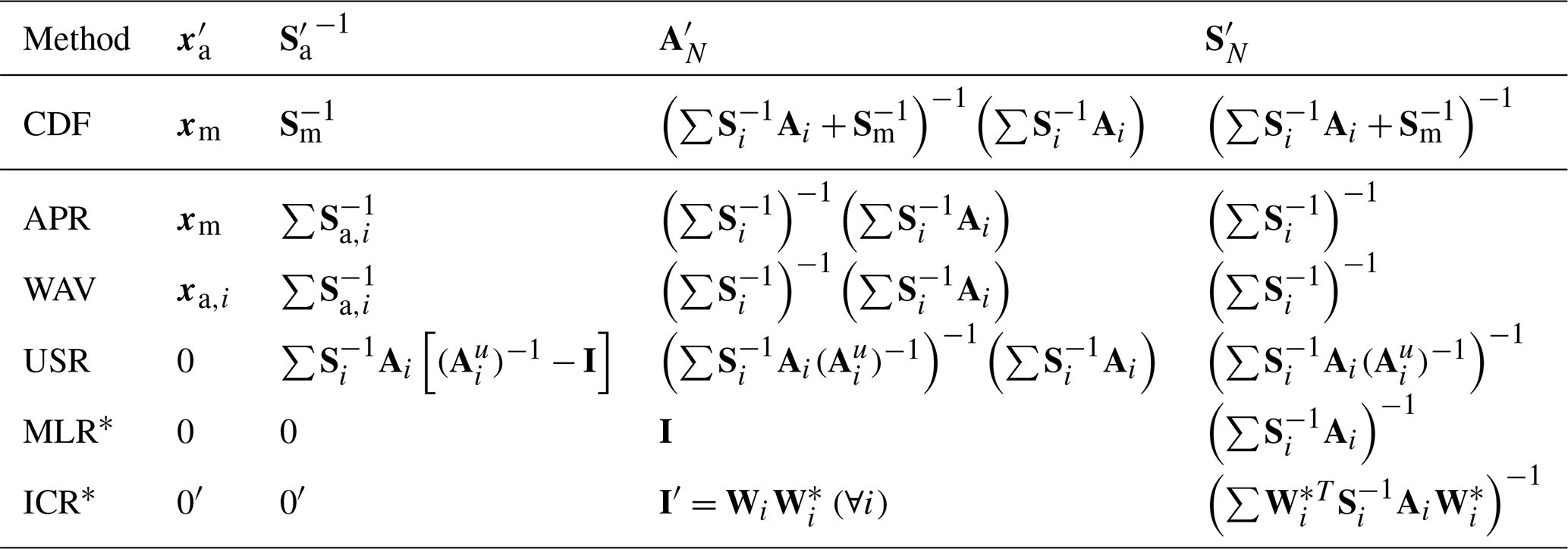
^* Not applied in this work.

Instead of replacing prior information while combining retrieved profiles, the CDF framework also allows removing prior information by appropriate choices of the new a-priori profile and constraint (Keppens et al., 2019). Upon setting the new prior profile to zero (${\mathit{x}}_{\mathrm{a}}^{\prime }=\mathrm{0}$), one essentially has two options for the new prior constraint ${{\mathbf{S}}_{\mathrm{a}}^{\prime }}^{-\mathrm{1}}$. It is either set to zero, or it is chosen in such way that the resulting averaging kernel matrix ${\mathbf{A}}_N^{\prime }$ has unit sensitivity, i.e. having all matrix row sums adding up to one and hence mimicking a Philips–Tikhonov-like retrieval. In both cases, the output profile does not effectively contain any prior information. The first option essentially corresponds to setting zero weight (or, equivalently, infinite uncertainty) to the a-priori profile during the retrieval process. In the CDF formulation, this translates into a deconvolution of the initially retrieved profiles to their maximum likelihood representation (MLR, Rodgers, 2000), as again becomes clear for a single retrieved profile:

$$\begin{array}{}\text{(6)}& {\mathit{x}}_{\text{MLR}}^{\prime }={\mathbf{A}}^{-\mathrm{1}}\left[\mathit{x}-(\mathbf{I}-\mathbf{A}){\mathit{x}}_{\mathrm{a}}\right]\end{array}$$

This approach however involves an unstable averaging kernel inversion, hampering its direct implementation (Keppens et al., 2022). One way out is to perform the kernel deconvolution on a different vertical grid, which is chosen in such way that ${\mathbf{W}}^{*T}{{\mathbf{S}}_{\mathrm{a}}^{\prime }}^{-\mathrm{1}}{\mathbf{W}}^{*}=\mathrm{0}$ non-trivially, with W^* being the generalised pseudo-inverse of a regridding matrix W that converts the vertical grid z of x_a and x into ${\mathit{z}}^{\prime }=\mathbf{W}\mathit{z}$ of ${\mathit{x}}_{\mathrm{a}}^{\prime }$. In order to include this regridding operation into the complete data fusion operation, it is sufficient to replace each A_i by a matching ${\mathbf{A}}_i{\mathbf{W}}_i^{*}$ in Eqs. (1)–(3) (Ceccherini et al., 2022). The result is called the information-centred representation (ICR, von Clarmann and Grabowski, 2007), as the single output profile ${\mathit{x}}_N^{\prime }$ has one independent retrieval degree of freedom at each vertical level by construction, and hence ${\mathbf{A}}_N^{\prime }$ equals the unit matrix (on the reduced vertical grid). Yet this representation yields high uncertainties for nadir ozone profile retrievals (Keppens et al., 2022). This work therefore sticks to the second option, which results in a fused averaging kernel matrix with unit-sensitivity. It is in principle obtained by resmoothing the MLR solution with the averaging kernel matrix A^u that is itself row-scaled:

$$\begin{array}{}\text{(7)}& \begin{array}{rl}{\mathit{x}}_{\text{USR}}^{\prime }& ={\mathbf{A}}^u{\mathit{x}}_{\text{MLR}}^{\prime }={\mathbf{A}}^u{\mathbf{A}}^{-\mathrm{1}}\left[\mathit{x}-(\mathbf{I}-\mathbf{A}){\mathit{x}}_{\mathrm{a}}\right]\\ & =(\mathbf{A}\mathit{u}{)}^{-\mathrm{1}}\left[\mathit{x}-(\mathbf{I}-\mathbf{A}){\mathit{x}}_{\mathrm{a}}\right]\end{array}\end{array}$$

where the last equation follows from the definition of the unit-sensitivity averaging kernel matrix: ${\mathbf{A}}^u=(A\mathit{u}{)}^{-\mathrm{1}}\mathbf{A}$, with u the vertical unit vector (Keppens et al., 2019). It is straightforward to demonstrate that within the CDF framework this unit-sensitivity representation (USR) is obtained by choosing ${{\mathbf{S}}_{\mathrm{a}}^{\prime }}^{-\mathrm{1}}=\sum {\mathbf{S}}_i^{-\mathrm{1}}{\mathbf{A}}_i\left[({\mathbf{A}}_i^u{)}^{-\mathrm{1}}-\mathbf{I}\right]$, which lies in between the APR and MLR constraints as can be expected: ${\mathbf{A}}^{-\mathrm{1}}-\mathbf{I}\ge ({\mathbf{A}}^u{)}^{-\mathrm{1}}-\mathbf{I}>\mathrm{0}$ (for each profile). In contrast with the MLR and ICR approaches, the USR profile and its covariance matrix, again see Tables 2 and 3, are well-defined (at least in theory).

Eventually, because of the difficulties that come with the MLR and ICR methods as mentioned above, two CDF-based vertical profile harmonisation methods are considered in this work, being the direct a-priori profile replacement (APR) and the unit-sensitivity representation (USR). Both are compared with the weighted average (WAV) profile, in order to verify whether the ozone profile data harmonisation reduces the inter-product dispersion (IPD) between the selected products (also see next section). Note that in practice, in order to strongly reduce data processing in terms of matrix multiplications, one can opt for applying only WAV data fusion first, and replacing the prior information in the single Level-3-like WAV profile x_N afterwards. This would mean making use of the single-profile Eqs. (4) and (7) for APR and USR, respectively, upon insertion of x_N and the weighted average prior profile x_a,N and averaging kernel matrix A_N. The only difference with the single-shot application of the complete data fusion framework is in the approximation of weighted mean multiplications by multiplications of weighted means. E.g., a term A_Nx_a,N instead of (Ax_a)_N appears in the APR method, yielding differences at the percentage level. This simplified approach is hence adopted in this work. Upon calculating these weighted averages within monthly 1°×1° boxes, the profiles (including pressure) and matrices of each pixel are limited to their mutual non-NAN values. Finally, in order to account for outliers due to averaging kernel oscillations, harmonised tropospheric ozone column values that deviate by more than 90 % from the corresponding WAV column are rejected from our analysis.

4.2 Performance

In order to assess the performance of the APR and USR harmonisation approaches as applied to the Level-2 nadir ozone profile data, we compare time series of zonal to global monthly means and IPDs before and after harmonisation for three tropospheric ozone columns, obtained from the profiles by integration up to the three top level definitions described in Sect. 3. At first instance, we look at near-global (60° N–60° S) one-to-one comparisons for all nadir profilers, for their respective mutual spatiotemporal domains (monthly grid boxes). Figure 2 summarises how much the spatiotemporally averaged relative difference between each product pair changes upon going from WAV to APR (below diagonal) and to USR (above diagonal), expressed in terms of the ratio, in %, between the products' mean difference before and after harmonisation, for all three top level definitions combined. This means that for values below 100 %, the harmonised products are closer to each other than the weighted averages, while the opposite is true for the values above.

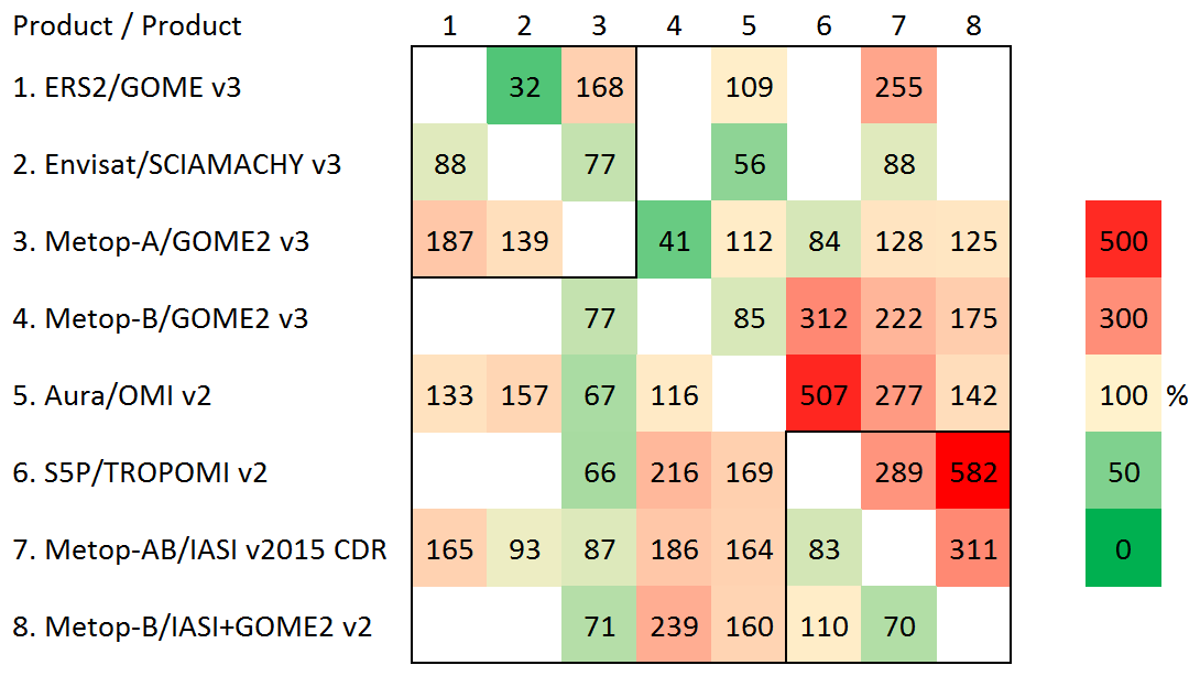
Figure 2 Spatiotemporally averaged relative difference between each product pair upon going from WAV to APR (below diagonal) and to USR (above diagonal), expressed in terms of the ratio, in %, between the products' mean difference before and after harmonisation, for all three top level definitions combined. For values below 100 % (in green), the harmonised product monthly means are closer to each other than the weighted averages, the opposite is true for the values above (in red). The diagonal and combinations without temporal overlap are empty. The top-left and bottom-right three-by-three boxes indicate the combinations that are used for Figs. 3 and 4, respectively.

Figure 2 demonstrates that the two ozone profile harmonisation approaches outlined above do not unambiguously reduce the averaged satellite-to-satellite differences. Most of these results, however, might not be a big surprise: As the five RAL profile products (numbers 1–5 in Fig. 2) originate from common prior profiles and constraints, it is to be expected that a prior profile replacement without retrieval re-optimisation, also see Keppens et al. (2019), increases their IPD (more values above 100 % below the diagonal). On the other hand, these products additionally having similar retrieval sensitivities in the troposphere, effectively removing the prior profile information from them reduces their IPD (more values below 100 % above the diagonal). The opposite is observed for the inter-product differences of the very different TROPOMI, IASI-AB, and IASI+GOME-2B retrievals (numbers 6–8). As these have both very different prior information (profiles and constraints) and tropospheric sensitivities, the APR method on average improves the agreement between their tropospheric ozone values, while the USR method, being largely dependent on the vertical sensitivity, fails to do so.

The opposing harmonisation performance between the common-prior RAL retrievals and the different-prior TROPOMI, IASI-AB, and IASI+GOME-2B products is further explored in Figs. 3 and 4, respectively. The first depicts time series of monthly global mean tropospheric ozone columns for the overlapping period (January 2007–June 2011) of GOME, SCIAMACHY, and GOME-2A (corresponding to the top-left box in Fig. 2), restricted to their common spatiotemporal sampling and for the three selected tropospheric top level definitions. The second does the same for the overlapping period (May 2018–December 2022) of TROPOMI, IASI-AB, and IASI+GOME-2B (corresponding to the bottom-right box in Fig. 2). The second to fifth rows of these figures contain the prior profile columns (PRI), weighted-averaged retrieved columns (WAV), harmonised columns using a-priori profile replacement (APR), and columns in their unit-sensitivity representation (USR), respectively, all in Dobson Units (DU). The first row (ΔSMOD) shows the difference between the CAMSRA model data x_m (black dashed lines) before and after averaging kernel smoothing. The latter is given by ${\mathit{x}}_{\mathrm{m}}^{\prime }=\mathbf{A}{\mathit{x}}_{\mathrm{m}}+(\mathbf{I}-\mathbf{A}){\mathit{x}}_{\mathrm{a}}$ (Keppens et al., 2019) and the difference ${\mathit{x}}_{\mathrm{m}}-{\mathit{x}}_{\mathrm{m}}^{\prime }$ hence captures the retrieval's vertical smoothing error as estimated by the model (Rodgers, 2000). As a function of time, this difference ΔSMOD then shows to what extent temporal changes in the averaging kernels (and thus retrieval sensitivity) affect the product time series (Pope et al., 2024). ΔSMOD will increase when the retrieval overall loses sensitivity in time, as is e.g. the case for GOME-2A and TROPOMI (yet note the dependence on the tropopause definition).

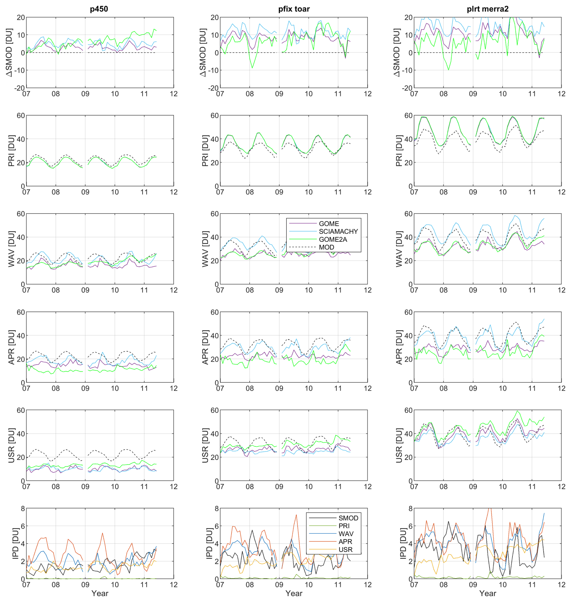
Figure 3 Evaluation of nadir ozone profile harmonisation for the overlapping period (January 2007–June 2011) of GOME (purple), SCIAMACHY (blue), and GOME-2A (green), restricted to their common spatiotemporal sampling. The first row shows the difference between the CAMSRA model data (black dashed lines) before and after averaging kernel smoothing. The second to fifth rows contain global mean tropospheric ozone time series for the prior profile columns (PRI), weighted-averaged retrieved columns (WAV), harmonised columns using a-priori profile replacement (APR), and columns in their unit-sensitivity representation (USR), respectively, all in DU. The last row depicts the IPD [DU] for each of the rows above. The PRI dispersion here roughly equals zero as all three products result from essentially the same RAL algorithm and prior input. The three columns correspond to the three selected tropospheric top level definitions.

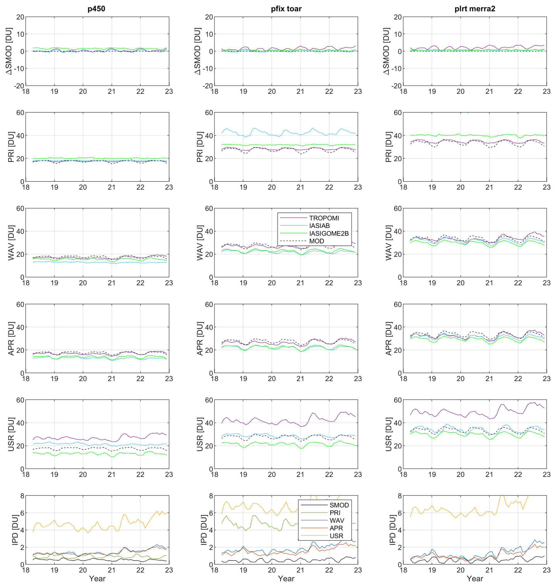
Figure 4 Same as Fig. 3 but for the overlapping period (May 2018–December 2022) of TROPOMI (purple), IASI-AB (blue), and IASI+GOME-2B (green), restricted to their common spatiotemporal sampling. Note that the IASI-AB PRI data is just above 60 DU for the lapse-rate tropopause definition (third column).

The last rows of Figs. 3 and 4 depict the IPD for each of the rows above. The smoothed model (SMOD) dispersion (in black) as such mimics the actual retrieval dispersion only, with the model acting as an observed state that is identical for all products. It should be close to or below the WAV dispersion (in red), as the latter also contains spatiotemporal sampling differences. This is indeed the case for both product triplets. For well-constrained retrievals, one moreover expects the dispersion between the APR harmonised products to be in between the SMOD and WAV dispersions, as the a-priori profile replacement method substitutes part of the initial retrievals by (smoothed) model data. Figure 4 shows that this is consistently the case for the different-prior products. It does not seem to hold for the RAL products for reasons explained above (essentially starting from a common prior already). The IPD statistics in the bottom rows of Figs. 3 and 4 nevertheless confirm the results in Fig. 2: For the triplet of common-prior products, the IPD increases when going from weighted averages to APR harmonised products (119 %), but reduces for the USR harmonisation (69 %), despite losses in the capturing of the ozone seasonality. For the different-prior (and tropospheric sensitivity) products, on the other hand, the IPD overall decreases when going from WAV to APR (87 %), but increases for WAV to USR (395 %). Note that the temporal oscillations in Fig. 3 are due to the coarse spatial resolution (large ground pixel sizes) and reduced global coverage of the three datasets involved. They contribute about 0–5 Level-2 profiles per Level-3 grid cell, while this is of the order of hundreds for the high-resolution profilers in Fig. 4.

Finally, Fig. 5 summarises the dispersion on the difference (thus here as an estimator of uncertainty, not IPD) between monthly time series of satellite and Level-3-like ozonesonde tropospheric columns for four nadir profile products (OMI, TROPOMI, IASI-AB, and IASI+GOME-2B) and for two tropospheric top level definitions (fixed 450 hPa pressure and the lapse-rate tropopause). For each data point, the satellite data time series is limited to the single grid cell covering the respective ground station (43 in total, sorted north to south). The dispersions on the satellite-ground difference time series have been calculated for the satellite weighted averages (WAV) and both harmonised profile products, APR and USR. The 5–15 DU dispersion results in Fig. 5 are much in agreement with the values presented above, although here we are looking at dispersions within (and not between) difference time series. As before, the USR harmonisation effectively works for the lower-resolution (both horizontal and vertical) RAL retrieval products with an order of 10 % difference dispersion reduction, while it does not for the other products. The APR method slightly benefits (by about the same percentage) the higher-resolution TROPOMI and (combined) IR retrievals yet performs poorly for OMI. The dispersion however again shows a remarkable meridian dependence, with smaller values and harmonisation effects in the Southern Hemisphere, except for the USR applied to IASI-AB (Sepang airport, San Cristobal and Nairobi are roughly at the Equator).

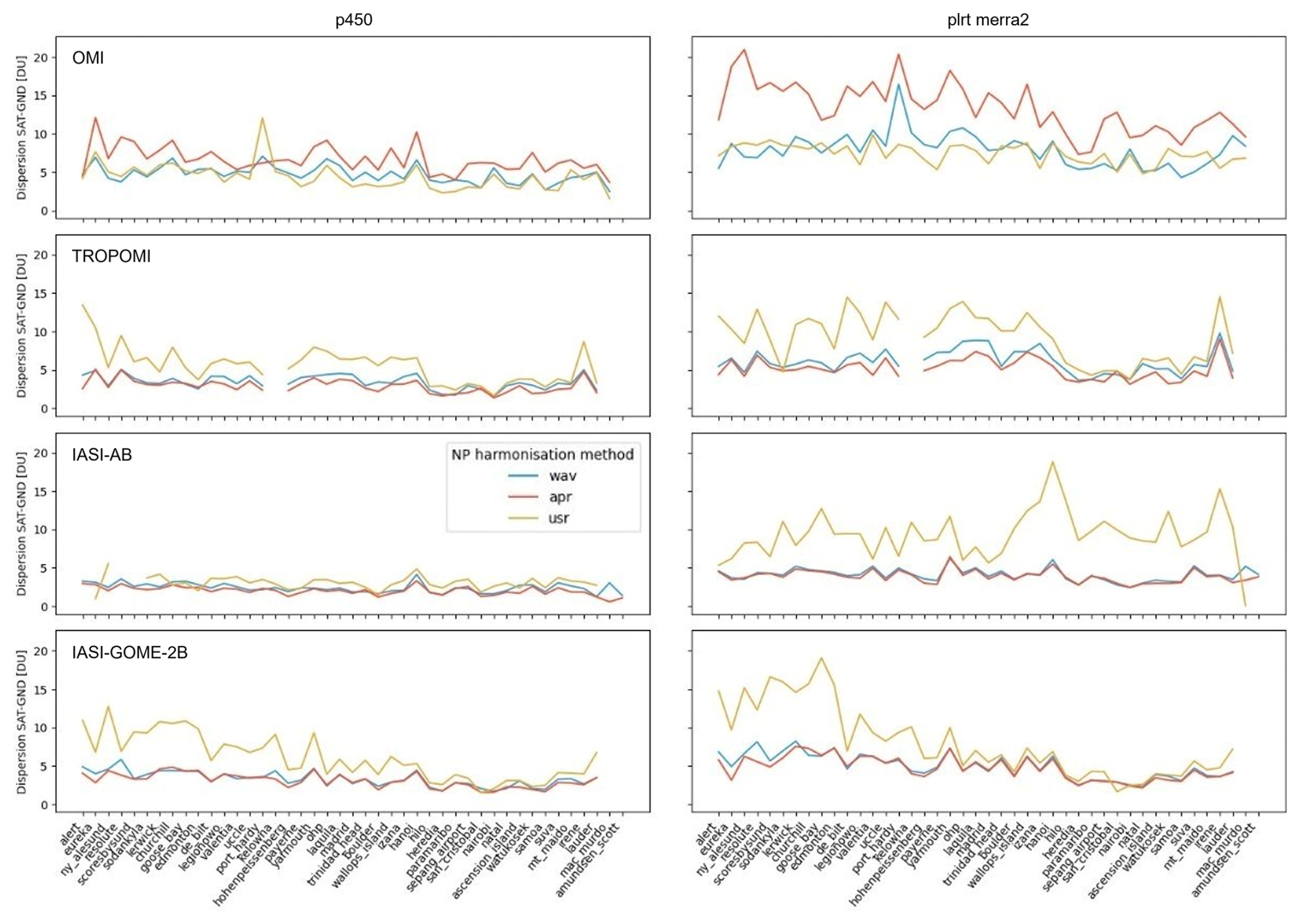
Figure 5 Dispersion on the difference between monthly time series of satellite (SAT) and Level-3-like ozonesonde (GND) tropospheric columns for four nadir profile products (OMI, TROPOMI, IASI-AB, and IASI+GOME-2B in rows, respectively) and for two tropospheric top level definitions (columns, 450 hPa fixed pressure level left and lapse-rate tropopause right). For each data point, the satellite data time series has been limited to the grid cell containing the respective ground station (sorted Arctic to Antarctic in each plot).

5 Column harmonisation

Two well-established approaches exist to harmonise the differences in the top level pressure p of residual satellite tropospheric (ozone) column products c that do not have averaging kernel information available (Gaudel et al., 2024). Accidentally in agreement with our selection of profile harmonisation methods, one of these makes use of reanalysis data as a transfer standard, while the other does not.

A first method computes the column-averaged ozone volume mixing ratio XO3 as $c/(p_{\mathrm{0}}-p)$ up to a constant $g_{\mathrm{0}}{M}_{\text{air}}/N_{\mathrm{A}}$ (combining the surface gravity g₀, the dry air molar mass M_air, and Avogadro's constant N_A). This expression as such ignores the vertical dependence of Earth's gravitational pull g and the presence of water vapour in air, but the induced overestimation of XO3 is at most +1 % only. This approach only provides a complete harmonisation of satellite products with different top levels p when and where the tropospheric ozone VMR profile is altitude-independent (Gaudel et al., 2018, 2024). One advantage, however, is that this method only requires additional knowledge of the surface pressure (p₀) and is therefore not limited by the spatiotemporal domain and data quality of a transfer standard.

A second method takes into account that ozone is not evenly distributed across the vertical domain of the reported column. It provides a correction of the vertical extent (p₀…p) of a given tropospheric column by adding (or subtracting) an ozone profile from a transfer standard (here CAMSRA) that is vertically integrated between p and another top level p^′. Prior to this, the profile of the transfer standard is scaled so that its column for top level p matches that of the satellite c, for each horizontal grid cell and timestamp. While doing so reduces biases between transfer standard and satellite, it also imprints measurement uncertainty (and its spatiotemporal structure) of the satellite onto the transfer standard. The harmonisation equation becomes $c^{\prime }=c+(c_{\mathrm{m}}^{\prime }-c_{\mathrm{m}})(c/c_{\mathrm{m}})=c(c_{\mathrm{m}}^{\prime }/c_{\mathrm{m}})$. This fill-in method relies on the availability of both the surface and top level pressures, and of the model columns c_m and $c_{\mathrm{m}}^{\prime }$ that are obtained from the model profile by vertical integration over p₀…p and p₀…p^′, respectively.

This work focuses on the second method only, as it captures vertical changes in tropospheric ozone (corrections) and hence is more suitable for vertically integrated tropospheric ozone column assessments. These are addressed in the next section, for harmonised ozone profiles and columns combined.

6 Effect on ozone assessments

The previous sections return four harmonisation approaches, two for the column products and two for the profile products, with one option involving reanalysis data for each. Given the performance results, however, we limit ourselves to the harmonised data including model-constraining here, i.e. APR and the fill-in method. We consider the tropospheric ozone column between surface and thermal tropopause (derived from MERRA2 temperature fields) as common top level, following a guideline from the TOAR-II community. We compare near-global maps and time series of original vs. harmonised satellite column data, and verify whether the spatiotemporal IPD is reduced upon harmonisation.

6.1 Multi-annual mean spatial distribution

Figure 6 maps the distribution of five-year mean near-global (2018–2022, 60° N–60° S) tropospheric ozone columns from the fourteen satellite datasets with temporal coverage in that period¹, before harmonisation. CAMSRA has been added for reference. The gaps that appear in the maps of GOME-2A/B are due to screening of the south-Atlantic anomaly (Finlay et al., 2020). Figure 7 depicts the same 2018–2022 multi-annual mean maps after harmonisation, using the APR method for the Level-2 profile products and the CAMSRA fill-in method for the Level-3 column products, with the MERRA2 thermal tropopause as common top level. From these 2018–2022 mean maps ${\overline{c}}_i(\mathit{\varphi },\mathit{\lambda })$, we calculate the IPD for each grid cell $s(\mathit{\varphi },\mathit{\lambda })=\sqrt{{\text{Var}}_i\left[{\overline{c}}_i(\mathit{\varphi },\mathit{\lambda })\right]}$ as an indicator of the dis/agreement between satellite datasets $\left\{{\overline{c}}_i\right\}$. To find out about possible improvements in the small-scale spatial structure we also consider the IPD of the spatial anomalies with respect to the near-global mean over the same time period (60° S–60° N)²: $s_{\mathit{\delta }}(\mathit{\varphi },\mathit{\lambda })=\sqrt{{\text{Var}}_i\left[\mathit{\delta }{\overline{c}}_i(\mathit{\varphi },\mathit{\lambda })\right]}$, where $\mathit{\delta }{\overline{c}}_i={\overline{c}}_i(\mathit{\varphi },\mathit{\lambda })-{\overline{c}}_{i,\text{near-global}}$. Near-global mean columns before (red) and after (blue) harmonisation are shown in Fig. 9 for the same fourteen satellite data products and CAMSRA (see discussion below). Figure 8 displays the change upon harmonisation of the IPD ($\mathrm{\Delta }s=s_{\text{harmonised}}-s_{\text{not harmonised}}$) for the 2018–2022 mean distributions of the satellite data products, both with (Δs_δ, bottom row) and without (Δs, top) their respective near-global means subtracted. The IPDs are computed separately for six Level-2 profile products (left column), for eight Level-3 column products (middle) and for all fourteen datasets (right).

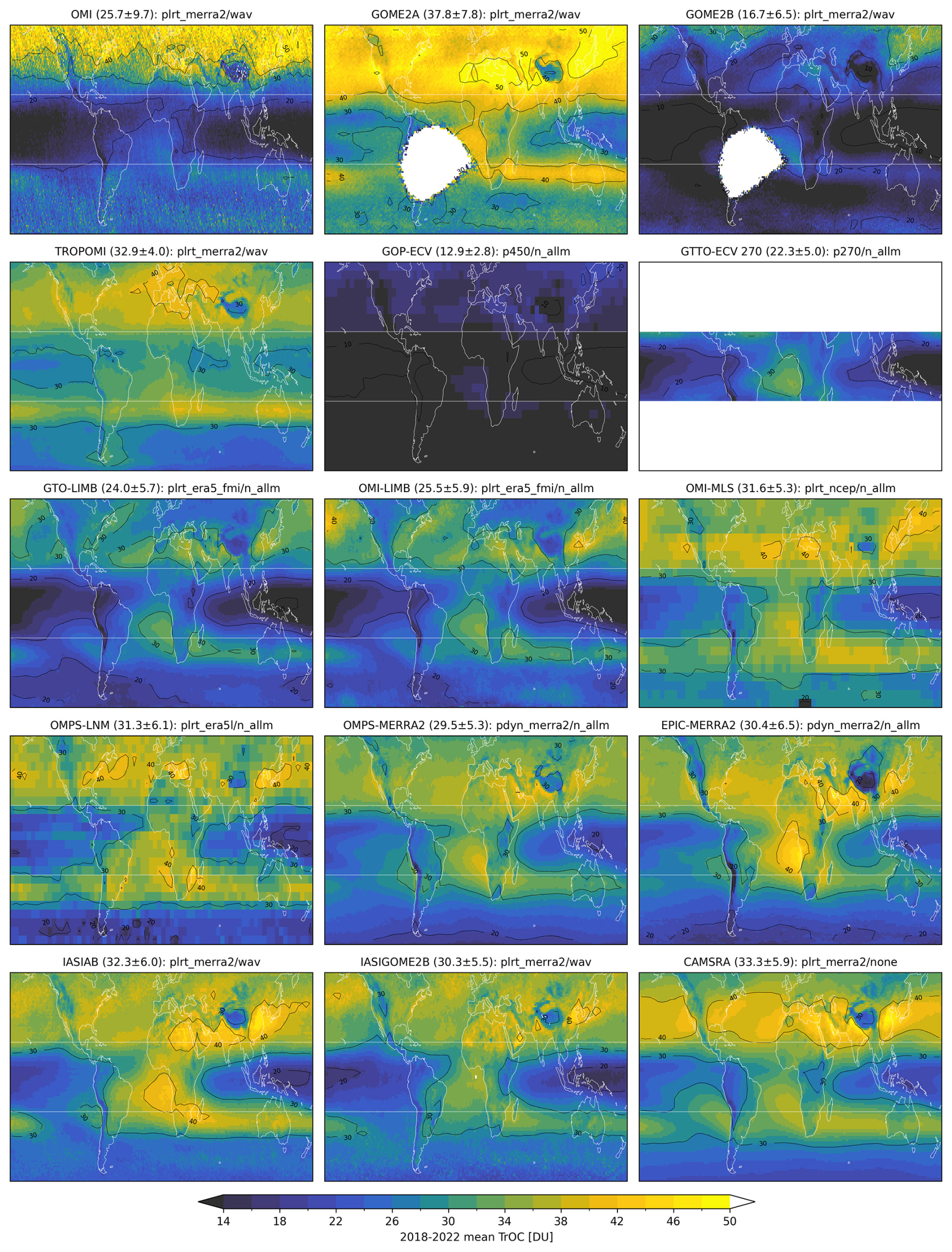
Figure 6 Multi-annual mean (2018–2022) tropospheric ozone column (TrOC) distribution of fourteen satellite data products and CAMSRA before harmonisation. Area-weighted mean and standard deviation of the near-global tropospheric column (60° N–60° S) are given between brackets.

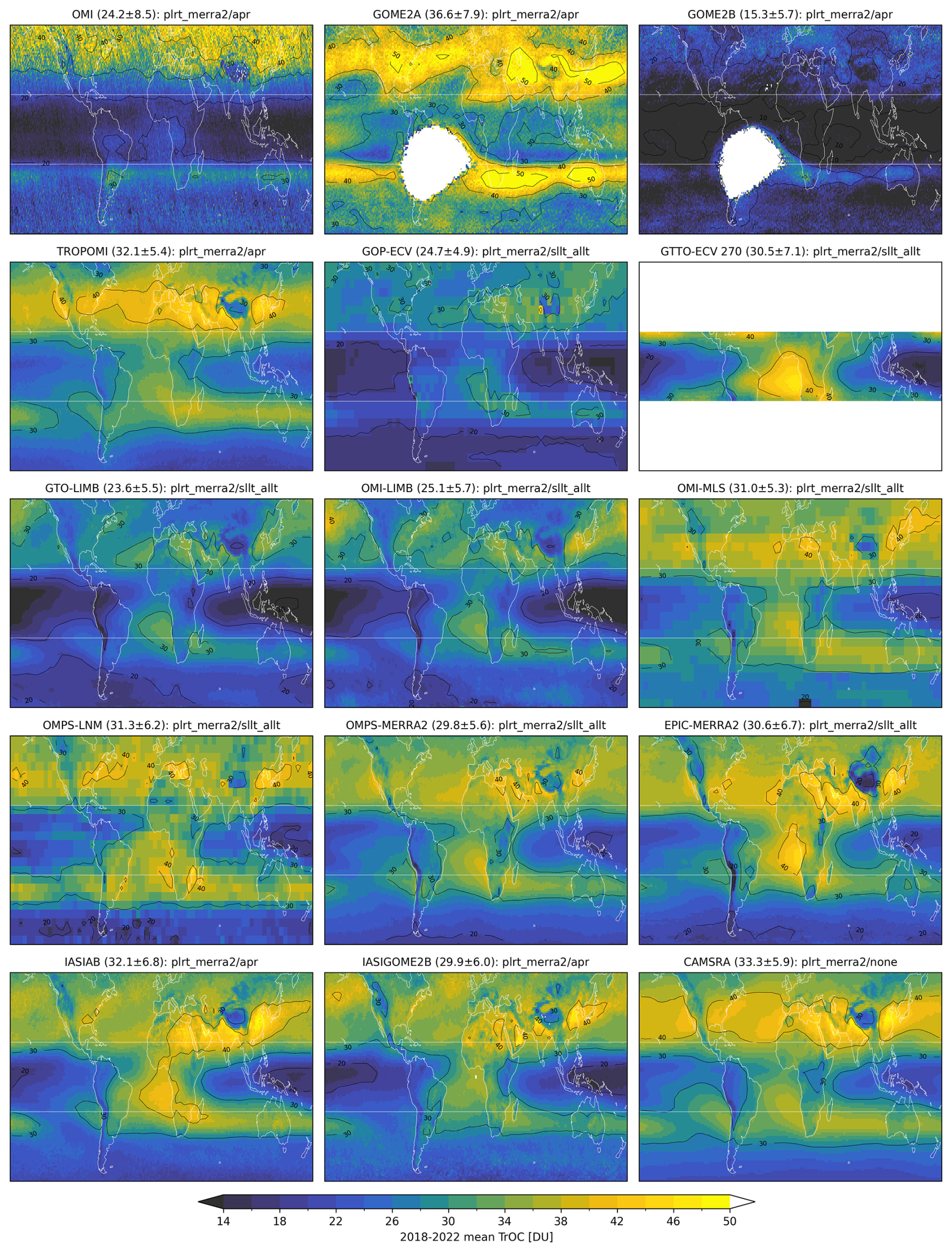
Figure 7 Multi-annual mean (2018–2022) tropospheric ozone column (TrOC) distribution of fourteen satellite data products and CAMSRA after harmonisation, using the APR method for the Level-2 profile products and the CAMSRA fill-in method for the column products. Area-weighted mean and standard deviation of the near-global tropospheric column (60° N–60° S) are given between brackets.

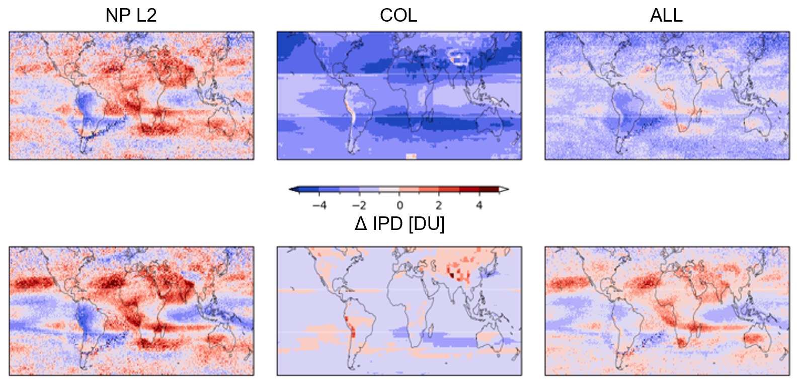
Figure 8 Change of the IPD (in DU) between satellite data sets upon harmonisation (after minus before), for the 2018–2022 mean of fourteen satellite data products. The top row shows the absolute tropospheric ozone column values, the bottom row their spatial anomaly (i.e. after subtraction of the 60° S–60° N mean). The left and middle columns differentiate the results for all fourteen datasets (on the right) between the Level-2 profile products and the Level-3 column products, respectively.

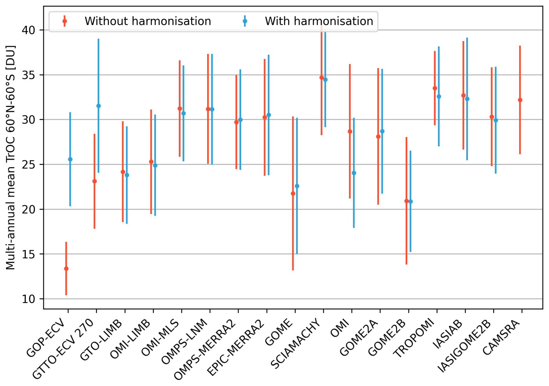
Figure 9 Near-global (60° N–60° S) multi-annual mean tropospheric ozone columns (TrOC) and dispersions before (red) and after (blue) harmonisation for all sixteen satellite data products and CAMSRA, over their full time series. The GTTO-ECV dataset covers 20° N–20° S and is not directly comparable to the near-global mean of the other datasets.

It is clear from Figs. 6 to 9, that the biggest overall change in tropospheric ozone column is found for the harmonised GOP-ECV and GTTO-ECV products whose initial top levels of, respectively, 450 and 270 hPa are located furthest away from the thermal tropopause. Therefore, the largest reduction (about 2–4 DU) in IPD is obtained for the residual column products (Fig. 8 top, middle). Also the IPD of the spatial anomalies decreases, though slightly (at most 1 DU), which implies that harmonisation allows slightly better constraints of small-scale spatial structure. The picture looks quite different for the APR harmonisation of the nadir profile products; their IPD reduction is mostly limited to parts of the Southern Hemisphere, with little differences between multi-annual columns or their spatial anomalies (Fig. 8, left). It is interesting to note that for the three RAL products involved (OMI, GOME-2A, GOME-2B), lower tropospheric ozone column values are found in the northern mid-latitudes after harmonisation (Figs. 6 and 7). Therefore, although their IPD is overall reduced by about 20 % upon APR, the latter also introduces a Northern Hemisphere bias with respect to the other three profile products here. When considering only the TROPOMI, IASI-AB, and IASI+GOME-2B datasets, the inter-product dispersion is reduced by 13 % upon APR harmonisation. Looking at all fourteen satellite products combined, the multi-annual mean IPD reduction upon harmonisation of the Level-3 column products prevails on the global scale. For the anomalies, however, IPD increases between the profile products mostly outweigh the IPD reductions between the column products upon harmonisation, especially in the Northern Hemisphere.

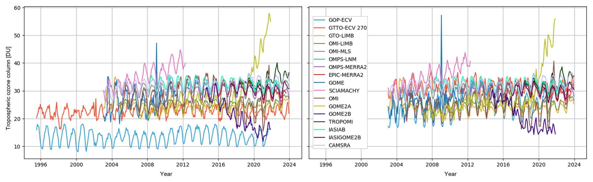
Figure 10 Near-global (60° N–60° S) tropospheric ozone column time series for all sixteen satellite data records and CAMSRA, both before (left) and after (right) harmonisation. Note that the latter is limited to the CAMSRA temporal domain (2003–2023).

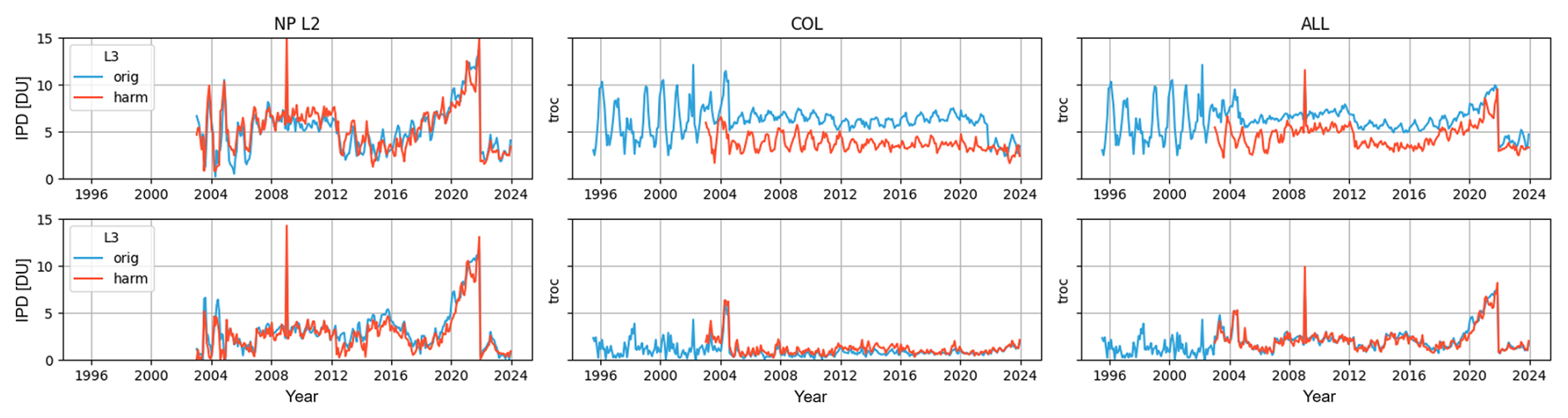
Figure 11 Inter-product dispersion (IPD) [DU] before (blue) and after (red) harmonisation, for the near-global time series of all sixteen satellite data products, both without (top) and with (bottom) their respective near-global means subtracted. The left and middle columns differentiate the results for all datasets (on the right) between the Level-2 profile products and the Level-3 column products, respectively.

6.2 Long-term changes and seasonal cycle

Figure 10 contains the near-global mean (60° N–60° S, as not all datasets cover the polar regions) time series for all sixteen satellite data records and CAMSRA, before (left) and after (right) harmonisation. The time domain of the latter is limited to that of the CAMS reanalysis needed for the harmonisation (2003–2023). Note that the considerable drifts observed for some UV-vis products are hardly affected by their APR harmonisation. Figure 11 depicts the temporal structure of the IPD, before (blue) and after (red) harmonisation, between eight Level-2 profile products (left), eight Level-3 column products (middle) and all sixteen satellite datasets (right). The top row is inferred from near-global mean tropospheric columns. The bottom row shows results after deseasonalisation of near-global mean columns to explore possible improvements of smaller-scale temporal structures.

The overall conclusion from Figs. 10 and 11 confirms what we have learned from the multi-annual mean maps: The largest reduction of IPD upon harmonisation, which is of the order of 3–4 DU or 40 %, is obtained from the top pressure matching of the tropospheric ozone column products (see GOP-ECV and GTTO-ECV in Figs. 9 and 10). It is clear that nadir ozone profile harmonisation using the a-priori profile replacement (APR) method does not consistently reduce the IPD in the temporal domain (Fig. 11, top-left). Only for the anomaly time series of the profilers, the IPD upon APR harmonisation seems globally reduced by about 1 DU or up to 10 %–20 % on average (Fig. 11, bottom-left, in agreement with our earlier findings), but only from 2012 onward (pointing at the limited success of APR harmonisation applied to the SCIAMACHY dataset). The IPD of the deseasonalised anomalies is not reduced after harmonisation of the tropospheric column products (Fig. 11, middle). This implies that the fill-in harmonisation of these products using CAMSRA does not alter the long-term time structure.

Also at the seasonal scale, there is no noticeable change in IPD before and after harmonisation either, as seen from Fig. 12, left and right, respectively. This figure depicts the IPD between all sixteen datasets for each month, by latitude band and on the near-global scale (60° N–60° S). It is hence clear that harmonisation of the profile and column datasets does not lead to better constraints of the seasonal cycle at the zonal to near-global level, although the seasonality of the IPD changes within some latitude bands, like 40–60° N and S. This seasonality, which is due to differences between sounders in their sensitivity to seasonal tropospheric ozone changes, may indeed be affected by changes in the vertical sensitivity upon harmonisation.

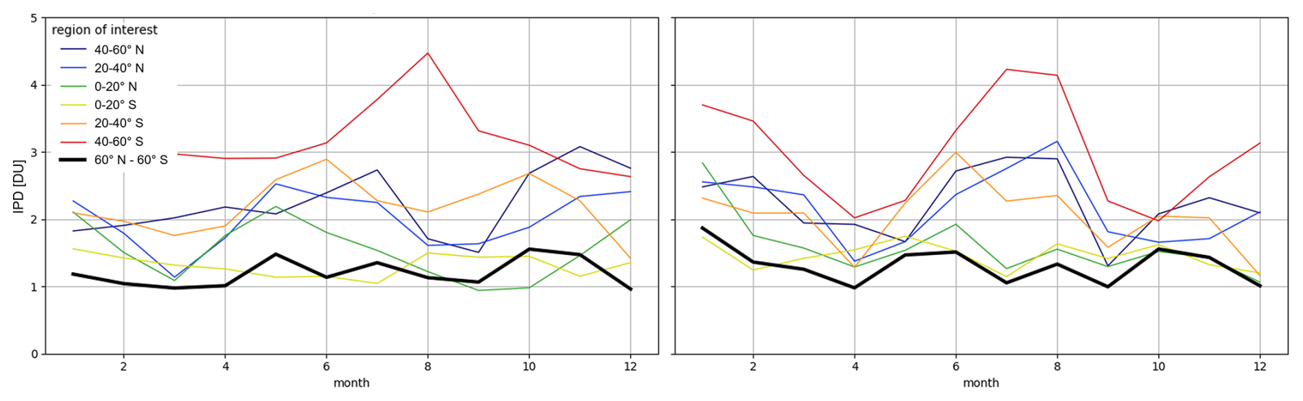
Figure 12 Zonal and near-global (60° N–60° S) seasonal cycles of the IPD [DU] for the full time series of all sixteen satellite data records, both before (left) and after (right) harmonisation. Note that the latter is limited to the CAMSRA temporal domain (2003–2023).

7 Conclusions

The main goal of this work is to address some of the challenges in interpreting the spatial distribution and long-term evolution of satellite ozone data records identified in the first Tropospheric Ozone Assessment Report (Gaudel et al., 2018). While TOAR concluded to a reasonably good agreement of the tropospheric ozone burden between satellite data records at the near-global, multi-annual mean level, it proved more challenging to assess the ozone burden at the regional scale, and especially to determine the sign and magnitude of long-term changes. These challenges were believed to be at least partially due to inherent differences between the satellite data in terms of unit representation, vertical smoothing, a-priori information, uncertainty characterisation, and spatiotemporal sampling, including the definition of the tropospheric top level as a major contributor. Our primary methodological objective is therefore to harmonise the vertical perspective of different ozone data records from satellites, for the two main classes of products that currently exist, and using the Copernicus Atmosphere Monitoring Service Re-Analysis (CAMSRA) as a transfer standard. The first class of tropospheric ozone products is obtained from nadir-viewing sounders, where spectral irradiance observations are retrieved into Level-2 vertical ozone profiles. The second class of products consists of the subtraction of a stratospheric component from total column retrievals, which yields Level-3-type tropospheric ozone column data.

We discuss in Sect. 4 how appropriate choices of new prior profiles and prior constraints within the Complete Data Fusion framework allow nadir ozone profile harmonisation (which requires the availability of averaging kernel matrices) in several ways. In order to avoid the known difficulties of the maximum-likelihood and information-centred representations, only the a-priori profile replacement (APR) and unit-sensitivity representation (USR) methods have been discussed in this work, with only the former making use of retrieval re-constraining using CAMSRA. Also for the tropospheric residual column products, two top level harmonisation approaches were discussed in Sect. 5: while the column-averaged volume mixing ratio (XO3) method assumes a flat vertical ozone distribution throughout the free troposphere, the fill-in method does not, and instead uses the CAMSRA profile shape to correct for the different vertical extent of the tropospheric columns. Using these methods, all products from both classes can be harmonised to obtain a tropospheric ozone column with a common top level, and common prior information where applicable. Eventually, our harmonisation assessment focused on those methods that are (re)constrained by the CAMS reanalysis, i.e. APR for the profile products and the fill-in method for the column data.

Our main research objective has been translated into two major research questions, addressing (1) whether the mutual consistency of satellite data sets, both in terms of their mean distributions and long-term changes, is improved by data harmonisation, and (2) whether this harmonisation does not worsen the agreement of the satellite data with ground-based reference observations. We consider monthly mean ozonesonde data obtained from the TOAR-II HEGIFTOM working group for the latter, and compared with the Level-3 (harmonised) satellite data for grid cells that contain one of the 43 launch sites. Note, however, that in contrast with the performance assessment for the nadir ozone profile harmonisation, there is little use in comparing pre and post harmonisation anchoring for the column datasets, given that the top level for the vertical ozonesonde profile integration is always matched with the top level of the satellite product.

For the nadir ozone profile products, the APR method reduces the IPD mainly for the high-resolution (both vertically and horizontally) TROPOMI and IR-based sounders, while the USR method mostly works for the UV-visible retrieval products by RAL with coarser resolution and having identical prior profiles initially. It became clear, however, that nadir ozone profile harmonisation does not fully reduce the IPD in a consistent way, not in space nor time. The IPD upon APR harmonisation is reduced by about 10 % on average, although with significant meridian dependence, when considering the four independent retrieval algorithms only. APR harmonisation additionally reduces the IPD between deseasonalised anomaly nadir profile datasets globally by about 1 DU or up to 10 %–20 % on average (but only post-SCIAMACHY, from 2012 onward). At the same time, APR harmonisation reduces the dispersion on the difference with respect to Level-3-like ozonesonde data by about the same percentage for the higher-resolution retrievals. The USR method effectively works for the lower-resolution RAL retrieval products with the same order of IPD reduction.

It could be questioned whether the roughly 10 % dispersion reduction, both in terms of inter-product consistency (IPD) and with respect to reference observations, that is obtained for the tropospheric ozone columns determined from harmonised nadir ozone profiles is worth the (not straightforward) harmonisation effort in practice, especially given its strong dependence on the native product resolution and its limited spatiotemporal consistency. Moreover, this 10 % value only partially alleviates the challenges to assess the present-day mean state and past changes in tropospheric ozone listed by TOAR. This implies that a substantial part of the inter-product differences are instrument and/or retrieval-specific (mainly including (drifting) measurement uncertainties, auxiliary data, and retrieval implementation) and hence need to be addressed at Level-1 and Level-2 data processing, preceding harmonisation. On the other hand, when resources are available, the nadir ozone profile harmonisation framework allows disentangling and hence studying prior (constraint) choices, sensitivity degradations, and retrieval performances within inter-product discrepancies. Unfortunately, it has been proven difficult to effectively remove the prior information, including changing sensitivities, from nadir-retrieved tropospheric ozone columns, whereas this does seem to work properly for limb (ozone) profile retrievals (von Clarmann et al., 2015; Keppens et al., 2022).

Looking at the profile and residual column products combined, the column fill-in method correcting for different tropospheric top level definitions appears to bring the highest gain in terms of IPD reduction (up to 40 %). This gain, however, mostly disappears when looking at the IPD of the anomaly time series of the column products only, which suggests that the fill-in harmonisation using a reanalysis rather mimics a global-scale inter-product bias correction. One could therefore also opt to apply this method to the lowest subcolumn of (vertically coarse) nadir ozone profile retrievals, as done for the Level-3 GOP-ECV product in this work by its lack of averaging kernels. For products with broad averaging kernels (effective vertical retrieval extents covering many layers), the latter might even be the preferred option, as it minimises the intrusion of stratospheric retrieval information into the tropospheric ozone column assessment. This approach is therefore also foreseen in the TOAR-II satellite data assessment (end of 2025). The selection of the transfer standard for column fill-in harmonisation is however of importance as well, taking into account that the choice between a reanalysis or a climatology results in (spatio)temporal differences in the correction term that can reach up to 2 DU or 5 %–10 % of the tropospheric ozone column. The sixteen harmonised tropospheric ozone column datasets presented in this work, obtained with CAMSRA as transfer standard, will be considered in the TOAR-II satellite data assessment and are planned to become available for download through the Belgian TAPIOWCA project (long-Term Assessment, Proxies and Indicators of Ozone and Water vapour changes affecting Climate and Air quality, https://doi.org/10.18758/r7u4z0he, Keppens et al., 2025).