Validating physical and semi-empirical satellite-based irradiance retrievals using high- and low-accuracy radiometric observations in a monsoon-influenced continental climate

Are high-accuracy radiometric observations strictly indispensable for the validation of satellite-based irradiance retrievals, or might low-accuracy observations serve as adequate substitutes? Owing to the scarcity of sites with redundant radiometers, such inquiries have seldom been contemplated, much less subjected to systematic examination; rather, it has been customary to employ all accessible observations during validation, frequently with only minimal quality control. In this investigation, we address this question by validating two distinct sets of satellite-retrieved irradiance – one derived through physical methods, the other through statistical means – against collocated high- and low-accuracy observations. Departing from the majority of validation studies, which rely exclusively upon an array of performance measures, we advocate and implement a rigorous distribution-oriented validation framework, yielding more profound insights and more comprehensive conclusions. Beyond the validation methodology itself, the dataset utilized in this study is noteworthy in its own regard: It incorporates radiometric observations from the newly established and first-ever Baseline Surface Radiation Network (BSRN) station situated within a monsoon-influenced continental climate (specifically, the Dwa Köppen classification), in conjunction with irradiance retrievals from the Fengyun-4B geostationary satellite, which are likewise new to the community. The accumulated evidence strongly suggests that the use of low-accuracy observations as a reference in validating irradiance retrievals may entail significant risks, because the discrepancies they introduce can be of a magnitude comparable to the commonly accepted margins of error or improvement (approximately several W m⁻² or a few percent) upon which numerous scientific assertions depend.

1 Introduction

Gridded irradiance retrieved from onboard imagers of geostationary satellites constitutes the foundation of numerous endeavors in solar energy meteorology, among which solar resource assessment and forecasting stand out as the most representative (Yang and Kleissl, 2024). Solar resource assessment aims to quantify the long-term (over years or decades) availability and variability of irradiance, thereby enabling the estimation of the energy yield and the evaluation of the economic feasibility and bankability of solar energy projects prior to their deployment. Given that the establishment and maintenance of dense radiometer networks over extensive regions and prolonged durations has never been a practical undertaking, and given that modeled irradiance (such as that derived from numerical weather predictions and reanalysis) remains constrained by its limited accuracy, the use of satellite-retrieved irradiance is the industry-standard practice for such assessments (Sengupta et al., 2024; Yang et al., 2022b). Solar forecasting – across varying short-term scales (from seconds to days) – is indispensable for grid operators, who must reliably formulate generation schedules accounting for the variable and intermittent nature of solar power output. In particular, within the intra-day window of 0–4 h, the advection of (normalized) satellite-retrieved irradiance fields has been consistently demonstrated to be the most reliable strategy (Yang et al., 2022a; Sweeney et al., 2020). In these applications of solar energy meteorology, the assurance of quality in satellite-retrieved irradiance products is of paramount importance – a necessity that has given rise to a substantial body of validation studies (e.g., Elias et al., 2024; Wandji Nyamsi et al., 2023; Qin et al., 2022; Kosmopoulos et al., 2018).

Irradiance retrieval from the top-of-the-atmosphere reflectance and brightness temperature measurements can be categorized into physical and data-driven types, depending on whether the retrieval process incorporates radiative transfer (Huang et al., 2019). Given that the execution of line-by-line radiative transfer calculations for each individual pixel and time stamp is computationally prohibitive, accelerated calculations, such as using a lookup table (e.g., Huttunen et al., 2016; Lefèvre et al., 2013) or parameterization (e.g., Huang et al., 2018; Xie et al., 2016), are invariably adopted in practice. Although physical retrieval methods are firmly grounded in established theory (Liou, 2002), they are not without their difficulties; persistent challenges that lead to geographic displacement of clouds remain unresolved. On the other hand, data-driven retrieval techniques, which can be further subdivided into semi-empirical (e.g., Huang et al., 2025; Chen et al., 2022; Perez et al., 2002) and machine learning (e.g., Shi et al., 2025, 2023; Verbois et al., 2023) methods, offer ease of implementation and can, under favorable conditions, achieve accuracy rivaling that of physical methods. However, such accuracy is contingent upon the quantity and quality of ground-based observations and cannot be assured a priori. Indeed, data-driven techniques often leverage large datasets with lower quality due to limited instrument maintenance, and the model potentially learns measurement errors, such as those due to soiling or calibration drift. Documented instances also exist where machine learning models, owing to overfitting, have produced retrievals exhibiting unphysical values or behavior (Yang et al., 2022c). In any case, these inherent limitations of existing retrieval techniques underscore the necessity of formal validation of satellite-derived irradiance.

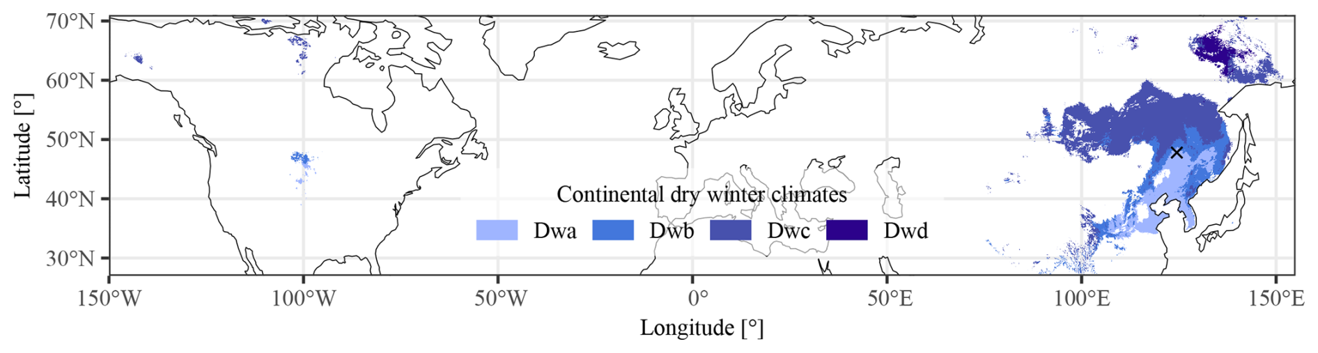
Figure 1 The geographical distribution of the continental dry winter climates. The location of the Qiqihar station is marked with a black cross.

The quality of satellite-derived irradiance varies as a function of spatial locations, time periods, and atmospheric conditions. Consequently, numerous validation efforts have adopted the practice of partitioning data samples into distinct groups representative of disparate climate classes, seasonal variations, and sky conditions. This kind of practice requires extensive data support, where the Baseline Surface Radiation Network (BSRN; Driemel et al., 2018; Ohmura et al., 1998), being the world's largest research-grade surface radiation monitoring network, has hitherto been an indispensable and reliable data source (Bright, 2019). BSRN began collecting surface radiation data in 1992 with nine initial stations. Ever since, the station listing has been dynamic, with some new stations being added and some older ones being closed; the present tally of active stations stands at 43. One of the initial aims of the network is to achieve coverage across major climate zones (Ohmura et al., 1998). However, as revealed in a global overview of multi-component solar radiometer monitoring stations (Jensen et al., 2025), the geographical distribution of climate zones and thus radiometric stations is highly uneven. For that, the establishment of BSRN in rarer climate zones has proven particularly challenging. For instance, Fig. 1 shows the geographical distribution of the continental dry winter climates, denoted by the Köppen symbol “Dw.” Until recently, its four subzones (Dwa to Dwd) remained entirely unrepresented within the BSRN framework, constituting a critical factor that precluded systematic investigation under such meteorological regimes. This impediment has now been partially remedied by the establishment of a new BSRN station in Qiqihar, China, in October 2023 – a development that permits, for the first time, rigorous inquiry into surface radiation characteristics within continental dry winter climates, including the validation of satellite-retrieved irradiance products.

Indeed, ground-based radiometric observations form an indispensable element in the validation of satellite-retrieved irradiance. The conventional validation methodology consists of computing aggregate performance measures, such as mean bias error (MBE), root mean square error (RMSE), or correlation, between retrievals and observations. However, these overall performance statistics suffer from well-documented limitations, such as interdependence or incompleteness, rendering conclusions drawn therefrom inherently questionable (Tian et al., 2016). To give perspective, two distinct sets of retrievals may yield identical MBE or RMSE values while exhibiting radically divergent temporal characteristics; this phenomenon is known as underdetermination (Tian et al., 2016) and has been more extensively documented in the forecasting literature (e.g., Yang and Perez, 2019; Vallance et al., 2017). Therefore, some have recommended using a more rigorous and systematic approach known as the distribution-oriented validation framework (Murphy and Winkler, 1987), which is receiving increasing acceptance in the solar community (Yang and Bright, 2020). The key philosophy of the distribution-oriented validation framework is to scrutinize the joint, marginal, and conditional distributions of prediction and observation, which allows visual and quantitative assessments of different aspects of quality, such as bias, association, calibration, refinement, or discrimination, through error decompositions (Yang et al., 2020). These aspects of quality possess clearly defined statistical complementarity, thereby offering more substantive insight than traditional measure-oriented validation, which often proves both subjective and inconclusive. To that end, this work employs the distribution-oriented validation framework, thereby furnishing a more comprehensive and analytically sound assessment of the irradiance products under examination.

Beyond questions of validation methodology lies a more fundamental concern regarding the quality of ground-based radiometric observations themselves. Since these observations serve as the ground truth, their uncertainties and biases, which are typically unaccounted for, inevitably undermine the confidence of any derived conclusions. Although the manufacturer-reported daily uncertainty of secondary-standard (i.e., Class A) radiometers is below 2 %, such singular numerical representations cannot possibly represent the true uncertainties encountered under actual field conditions. It has been reported that the difference among regularly calibrated thermopile radiometers can reach up to ±17 % at high zenith angles and under cloudy skies (Habte et al., 2016). Moreover, the impracticality of deploying redundant radiometers for repeated measurements compels reliance upon rigorous quality control (QC) procedures as the sole means of ensuring the validity of ground truth. Even so, most operational radiometric sites are limited to measuring the global irradiance component, and not the individual diffuse and beam components. This limitation renders certain QC tests inapplicable, most notably the three-component closure test, which verifies the agreement between measured global irradiance and the sum of its diffuse and beam constituents. These considerations lead us to a critical epistemological question: To what extent can observed validation deviations be properly attributed to limitations in the ground-based observations themselves, rather than to deficiencies in the satellite retrievals? This distinction is not merely technical but fundamental to the proper interpretation of validation results (see Sect. 10.4 of Sengupta et al., 2024).

Guided by the above preliminaries, the present investigation establishes three principal objectives: (1) conduct a systematic validation of physical and semi-empirical satellite irradiance retrievals under the monsoon-influenced dry-winter hot-summer continental climate (i.e., the Dwa Köppen climate), which is a climatic regime remarkably underrepresented in existing studies; (2) demonstrate the methodological superiority of distribution-oriented validation compared to conventional measure-oriented approaches; and (3) quantitatively assess the propagation of observational uncertainties from ground-based radiometers into validation outcomes. The organization of this paper proceeds as follows: Sect. 2 provides a comprehensive exposition of the datasets, their quality control procedure, and the formal validation methodology. Section 3 depicts the validation outcomes and discusses the implications of the quality of ground-truth on gridded irradiance validation. Section 4 synthesizes the principal findings and their broader implications.

2 Data and method

2.1 Data description

A total of four datasets are involved herein, among which two consist of ground-based radiometric observations, and the other two are satellite-retrieved irradiance. The two sets of ground-based observations are collocated. One set of ground-based observations comes from the BSRN Qiqihar (QIQ) station, which employs secondary-standard radiometers and represents high-standard radiometric practices. In contrast, the other set of ground-based observations comes from an operational station of the China Meteorological Administration (CMA), which uses a pyranometer from a Chinese manufacturer that is potentially associated with higher uncertainties than the secondary-standard ones. Notation-wise, we denote the high-accuracy set of observations as y_H, and the low-accuracy set of observations as y_L.

The two sets of satellite-retrieved irradiance are both derived from images captured by the Advanced Geostationary Radiation Imager (AGRI) on board the Fengyun-4B (FY-4B) satellite, which is the second of the latest-generation Chinese geostationary meteorological satellite series. To exemplify the physical retrieval algorithms, the official FY-4B irradiance product of the National Satellite Meteorological Center (NSMC) of CMA is considered. As for the statistical (or semi-empirical) retrieval, the product of Huang et al. (2023), which is based on a modified version of the Heliosat-2 method of Rigollier et al. (2004), is used without loss of generality. Similarly to the case of ground-based observations, the two sets of satellite-retrieved irradiance are denoted as x_P and x_S, respectively, with the subscripts denoting “physical” and “statistical.” In short, this work seeks to validate x_P and x_S using y_H and y_L, separately. The period of validation is one year from April 2024 to March 2025.

2.1.1 High-accuracy observations from the BSRN QIQ station

The BSRN QIQ station (47.7957° N, 124.4852° E, 170 m) is located in the monsoon-influenced dry-winter hot-summer continental climate, which has a symbol of “Dwa” under the Köppen climate classification. Given the geographical distribution of the Dwa climate, which is mostly in northeastern Asia, the surface radiation characteristics based on high-quality ground-based radiometers have rarely, if ever, been formally reported, thereby making this report unique and valuable.

Following the BSRN requirements, QIQ measures all three downward surface shortwave radiation components, as well as the downward longwave radiation, with a sampling rate of 1 s. For the global horizontal irradiance (GHI) and diffuse horizontal irradiance (DHI), CMP22 pyranometers from Kipp & Zonen are used, whereas a CHP1 pyrheliometer mounted on a SOLYS2 sun tracker is used to measure the beam normal irradiance (BNI). All radiometers are calibrated and regularly maintained. For more technical details of the QIQ station, the reader is referred to the recent work by Liu et al. (2025). It should be highlighted that the CMP22 pyranometers are ventilated but not heated, due to the high thermal offset observed during the winter of 2023 (the heaters have been switched off since then).

2.1.2 Low-accuracy observations from the CMA operational station

Compared to basic meteorological variables, such as temperature or precipitation, solar irradiance does not have the same degree of impact on daily human activities. Consequently, radiometers have hitherto been regarded as an additional feature in weather stations. For instance, CMA maintains more than 90 000 manned and unmanned weather stations, but only about 100 of them have radiometers installed (Yang et al., 2022b). Among these CMA operational radiometric stations, only a handful measure all three shortwave components, whereas most only measure GHI, including the Fuyu County Meteorological Bureau, within which the QIQ station is located. This GHI dataset, therefore, serves as an alternative version of ground truth for validating gridded irradiance retrievals.

The radiometer employed by the Fuyu Bureau is a DFN1 thermopile pyranometer by Huatron Environment, a Chinese brand. DFN1 is a first-class (i.e., Class B) pyranometer that has acquired the CMA's special technical equipment license for meteorological observation. According to the manufacturer, DFN1 has a spectral range of 300–3000 nm (200–3600 nm for CMP22), a response time of < 20 s (< 5 s for CMP22), and a temperature response of $\le \pm$2 % ($\le \pm$0.5 % for CMP22). The data is sampled at 2 s but only logged as 1 min averages. The DFN1 at the Fuyu Bureau is also equipped with an SRC228 ventilation unit. Through the CMA standard data and communication protocol, the 1 min data is transmitted to the central server in near real-time.

2.1.3 Physical irradiance retrievals from NSMC

The FY-4B satellite was successfully launched on June 3, 2021, and was located at 123.5° E on 10 June 2021, relocated at 133° E from 11 April 2022 to 31 January 2024, and positioned at its final position of 105° E on 5 March 2024. The NSMC official FY-4B irradiance product is developed by the Algorithm Working Group and consists of all three surface shortwave components. The retrieval algorithm is of a physical type, which, as mentioned in the introduction, is based on radiation transfer, accounting for all important radiation transfer physical processes in the shortwave range, including multiple scattering, absorption, and thermal radiation, to form a look-up table. More specifically, the observations from channels 1 to 6 of the FY-4B AGRI and the FY-4B L2 snow cover product are used to obtain the instantaneous state variable information of the atmosphere and the surface, mainly including atmospheric extinction parameters and surface reflectance. After determining the instantaneous state of the atmosphere and the surface, irradiance is estimated according to the pre-established lookup table, taking into account the sun–surface–satellite geometry.

FY-4B has 15 channels with a native resolution ranging from 0.5–4 km at nadir, depending on the channel. Since the retrieval algorithm uses multiple channels, the spatial resolution of the final product follows that of the lowest-resolution channel, which is 4 km. Temporally, AGRI completes a full-disc scan over each 15 min interval. The exact instant of AGRI passing the pixel corresponding to the QIQ station is not considered in this work. Instead, the time stamps follow the scan intervals. This slight asynchrony is unlikely to cause major offsets during validation, especially after hourly averages are formed.

2.1.4 Statistical irradiance retrievals using the modified Heliosat-2 method

Heliosat-2 is a well-known statistical irradiance retrieval technique that is primarily based on three components: (1) a clear-sky model, (2) a method to estimate cloud index from satellite reflectance observations, and (3) a mapping function from cloud index (ν) to clear-sky index (κ). Once the κ is obtained, GHI can be reconstructed by multiplying κ with the clear-sky GHI. The reader is referred to Appendix A for an extended explanation of the algorithm. In the work of Huang et al. (2023), the clear-sky GHI is estimated via the REST2 model, the cloud index is estimated from the Fengyun-4A (FY-4A) level-1 reflectance of the visible channel (0.65 µm), and the coefficients of the ν-to-κ mapping are determined based on 38 stations operated by the Chinese Ecosystem Research Network. Since only the visible channel observations are involved, the spatial resolution of the product is 0.5 km, which can reveal more granular spatial features without sacrificing much accuracy compared to a benchmark product – the Himawari-8 product developed by the Japan Aerospace Exploration Agency (Huang et al., 2023). On the other hand, the cloud shadow and edge reflectances are more pronounced for high-resolution retrievals, which can disturb the calculation of the cloud index.

In this work, the same retrieval technique is used to acquire GHI on a grid cell collocated with the QIQ station, with the only difference being the raw data source, which is FY-4B instead of FY-4A. As noted by Huang et al. (2025), one of the advantages of semi-empirical retrieval methods is the independence of satellite calibration information, which means that the previous algorithm can be applied “as is” without modification. It should be noted, however, that FY-4A is an experimental satellite with known fluctuations in radiometric performance and an irregular observation schedule (Zhong et al., 2021). In contrast, FY-4B demonstrates superior calibration stability, comparable to the GOES-R and Himawari-8/-9 satellites. The statistically retrieved irradiance also follows the observation schedule of FY-4B, which has a regular 15 min interval.

2.2 Data quality control and temporal alignment

To ensure the soundness of the outcome drawn from the validation exercise, the ground-based observations must first undergo quality control. Additionally, considering the differences in temporal resolutions of various datasets, it is vital to aggregate and align them temporally. These two aspects are described in this section.

2.2.1 Quality control routine for irradiance

The optimal QC procedure ought to provide a sufficient balance between the number of rejected inlier data points and the number of retained anomalous data points. In this work, the QC checks used by the International Energy Agency (IEA) PVPS Task 16 team are considered (Forstinger et al., 2021), which is based on the BSRN recommended routine (Long and Shi, 2008) with notable additions. Notation-wise, several well-known normalized indexes (or k indexes) are to be first defined, they are the clearness index $k_{\mathrm{t}}=G_{\mathrm{h}}/E_{\mathrm{0}}$, the beam transmittance $k_{\mathrm{b}}=B_{\mathrm{n}}/E_{\mathrm{0}n}$, the clear-sky index $\mathit{\kappa }=G_{\mathrm{h}}/G_{\mathrm{hc}}$, and the diffuse fraction $k=D_{\mathrm{h}}/G_{\mathrm{h}}$, where G_h, D_h, and B_n denote GHI, DHI, and BNI, respectively; G_hc is the clear-sky GHI; and E₀=E_0ncos Z is the extraterrestial GHI, with Z being the zenith angle.

The k indexes are normalized versions of various irradiance components. They are also very commonly used in radiation modeling, when the yearly and diurnal cycles of irradiance interfere with model fitting (Yang and Kleissl, 2024). Based on the k indexes, several QC tests can be formulated:

• k_b<k_t, for G_h>50 W m⁻², k_t>0, and k_b>0

• $k_{\mathrm{b}}<(\mathrm{1100}\mathrm{W}{\mathrm{m}}^{-\mathrm{2}}+\mathrm{0.03}\times \mathrm{altitude}\mathrm{in}\mathrm{m}.\mathrm{a}.\mathrm{s}.\mathrm{l}.)/E_{\mathrm{0}n}$, for G_h>50 W m⁻² and k_b>0

• k_t<1.35, for G_h>50 W m⁻²

• k<1.05, for Z<75° and G_h>50 W m⁻²

• k<1.10, for Z≥75° and G_h>50 W m⁻²

• k<0.96, for k_t>0.6, Z<85°, and G_h>50 W m⁻²

When the conditions specified by these tests are not met, the corresponding data points are flagged as “anomalous.”

Besides the k index tests, the extremely rare limits (ERL) test and the three-component closure test are also part of the QC routine. They are:

• −2 W m${}^{-\mathrm{2}}\le G_{\mathrm{h}}\le \mathrm{1.2}{E}_{\mathrm{0}n}{\cos }^{\mathrm{1.2}}Z+\mathrm{50}$ W m⁻²

• −2 W m${}^{-\mathrm{2}}\le D_{\mathrm{h}}\le \mathrm{0.75}{E}_{\mathrm{0}n}{\cos }^{\mathrm{1.2}}Z+\mathrm{30}$ W m⁻²

• −2 W m${}^{-\mathrm{2}}\le B_{\mathrm{n}}\le \mathrm{0.95}{E}_{\mathrm{0}n}{\cos }^{\mathrm{0.2}}Z+\mathrm{10}$ W m⁻²

and

• abs(δ)≤8 %, for Z<75° and G_h>50 W m⁻²

• abs(δ)≤15 %, for $\mathrm{93}\mathit{°}>Z>\mathrm{75}$° and G_h>50 W m⁻²

where $\mathit{\delta }=G_{\mathrm{h}}/(B_{\mathrm{n}}\cos Z+D_{\mathrm{n}})-\mathrm{1}$ is the decimal difference of the closure relationship. Last but not least, the tracker-off test is given by:

• $(G_{\mathrm{hc}}-G_{\mathrm{h}})/(G_{\mathrm{hc}}+G_{\mathrm{h}})<\mathrm{0.2}$, for Z<85°

• $(B_{\mathrm{nc}}-B_{\mathrm{n}})/(B_{\mathrm{nc}}+B_{\mathrm{n}})>\mathrm{0.95}$, for Z<85°

It should be noted that although G_hc and B_nc can be estimated via a clear-sky model, they are defined as G_hc=0.8E₀ and $B_{\mathrm{nc}}=(G_{\mathrm{hc}}-D_{\mathrm{hc}})/\cos Z$ herein, with D_hc=0.165G_hc.

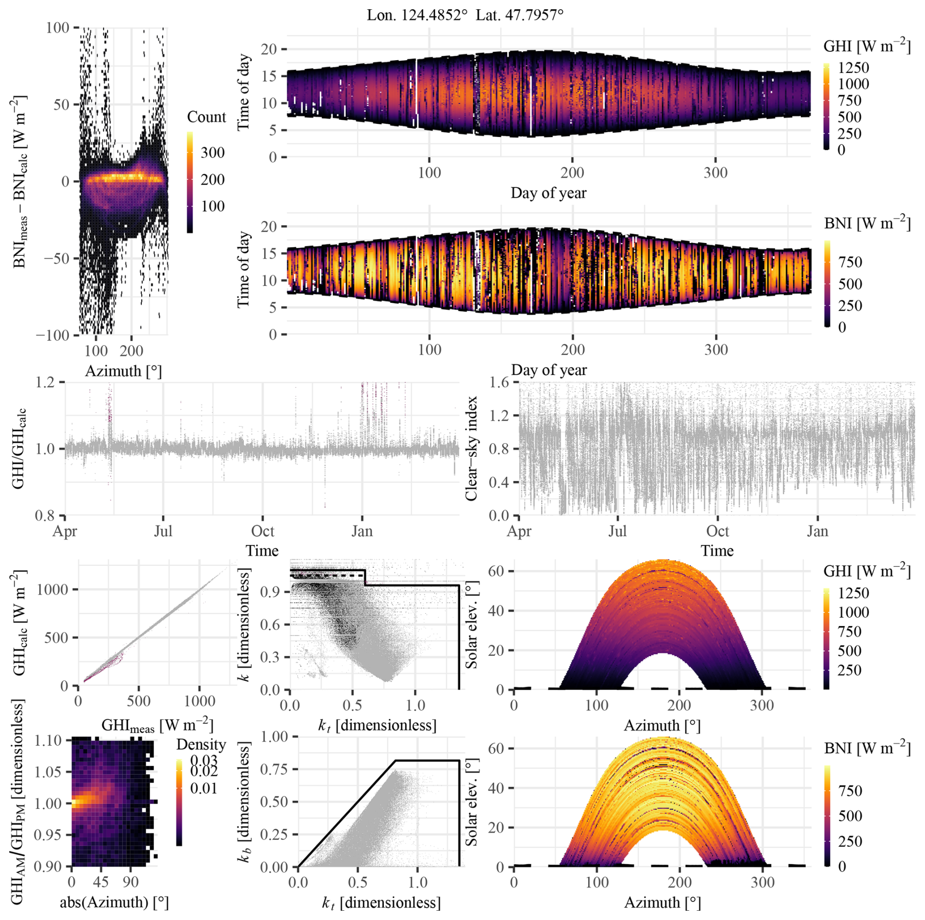
Figure 2 A multiplot depicting the quality of QIQ observations. Each subplot shows the result of a particular quality control test. For the detailed interpretation of each test involved here, the reader is referred to Forstinger et al. (2021).

The above QC routine requires all three irradiance components to execute, and thus can only be applied to the QIQ observations. As for the CMA observations, only the first line of the ERL test is applicable. All tests are performed on 1 min data, and the outcome is displayed in Fig. 2, which is known as a multiplot, as named by Forstinger et al. (2021), to whom the reader is referred for detailed interpretation. (There are several calculated quantities with subscript “calc” in this plot, which all result from the closure equation.) In short, the 1 min QIQ observations are of good quality with very few missing and rejected data points. Most of the rejected data points are due to (1) frost deposition on the glass cover of the pyrheliometer, (2) elevated thermal offsets in pyranometers, and (3) horizon shading by nearby buildings during winter sunsets. Although regular maintenance is conducted by the on-site staff, it is still difficult to entirely avoid data issues, again highlighting the importance of QC.

2.2.2 Data aggregation and temporal alignment

One year of 1 min observations corresponds to 525 600 samples, among which 239 879 are daytime samples – considering the higher directional uncertainty of pyranometers at low-sun conditions, daytime samples are defined as those with zenith angles ≤85°. The daytime samples from QIQ are passed through the above-mentioned QC routine, and 1510 (or 0.64 %) data points are flagged and thus rejected before aggregation. The non-flagged data are aggregated to a 15 min data interval using right-labeled timestamps, i.e., the time stamps correspond to the end of the aggregation interval. To ensure that each aggregated value can sufficiently represent the average condition of the corresponding intervals, only intervals with more than seven 1 min data points are considered valid. After aggregation, a total of 15 576 valid 15 min data points remain.

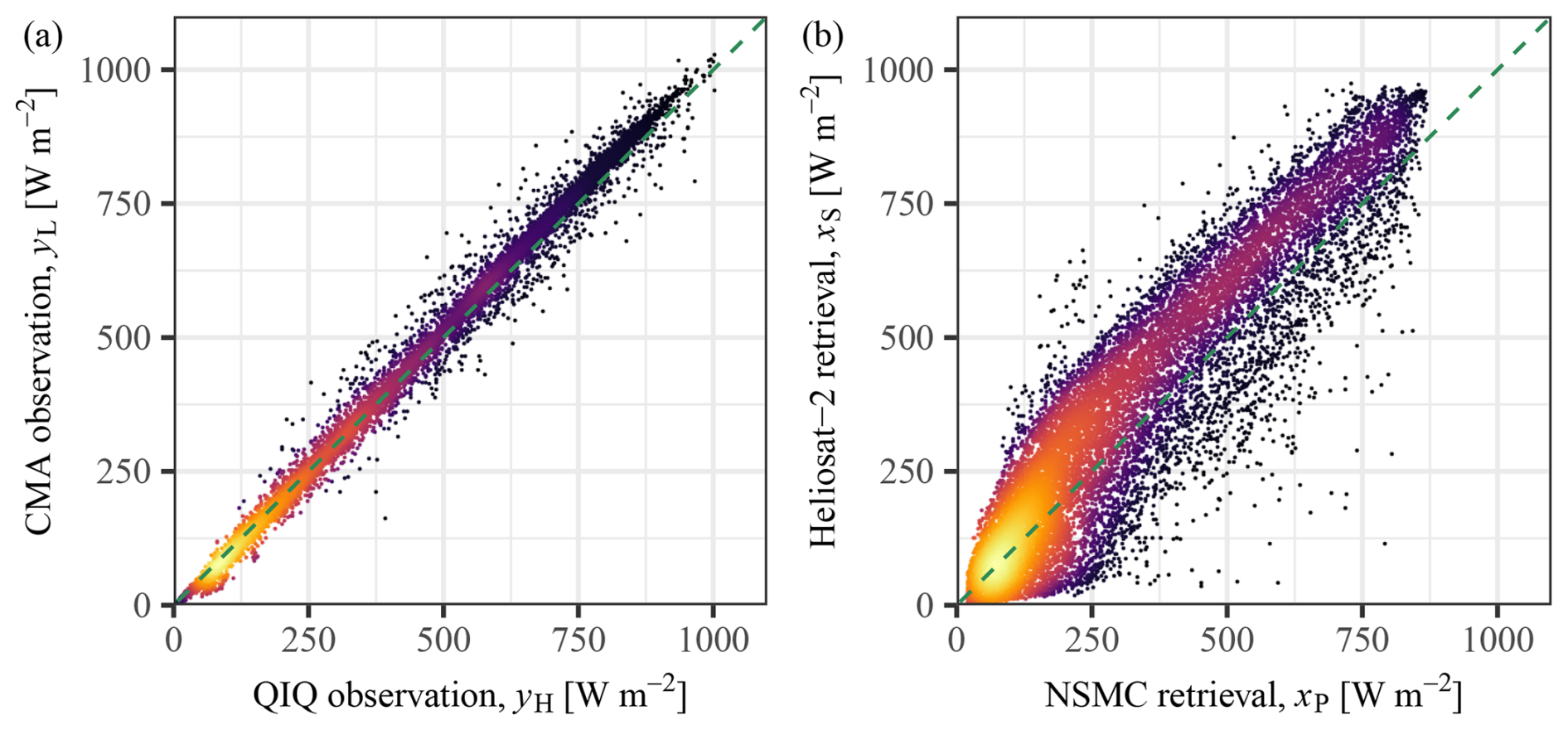
Figure 3 Scatterplots of (a) the low-accuracy CMA observations (y_L) against the high-accuracy QIQ observations (y_H) and (b) the Heliosat-2 statistical retrieval (x_S) against the NSMC's physical retrieval (x_P). Brighter colors signify higher sample density.

After processing the QIQ data (i.e., y_H), the 1 min CMA observations (i.e., y_L) are aggregated in the same fashion and appended to the QIQ data frame, alongside the two sets of 15 min-resolution retrievals (i.e., x_P and x_S). It is noted that both the CMA observations and the retrievals contain missing instances. A row-wise filter is thus applied to the data frame to remove incomplete timestamps, resulting in 14 595 final samples. Stated differently, all subsequent validation exercises are based on this 14 595×4 data frame, with the four columns being y_H, y_L, x_P, and x_S. Figure 3a shows the scatterplot between y_H and y_L, and the high- and low-accuracy observations have an exceptional agreement, with a Pearson correlation of 0.997 and a mean difference of 3 W m⁻². In contrast, the scatterplot between x_P and x_S, as depicted in Fig. 3b, shows substantial discrepancies and noticeable nonlinearity, with a correlation of 0.926 and a mean difference of 40 W m⁻², suggesting that one of these products has major technical issues that need to be further investigated.

2.3 An overview of the validation methodology

Validation of gridded products can be categorized into measure- and distribution-oriented approaches. Whereas the former employs a suite of performance measures and statistics to gauge the product quality, the latter examines the joint (or equivalently, the marginal and conditional) distributions of retrieval and observation. However, these two approaches are not mutually exclusive, as many performance measures can be written in terms of distributions, see Eqs. (1) and (2) below. Therefore, both approaches are introduced next and their outcomes reported in Sect. 3.

2.3.1 Measure-oriented validation

A majority of existing works on gridded irradiance validation use the measure-oriented approach, among which the MBE and RMSE are the most popular choices of performance measures (e.g., Yang and Bright, 2020; Sengupta et al., 2018). MBE is often reported because ensuring a low bias has the utmost importance in solar resource assessment, but high accuracy is not as critical (Perez et al., 2013). On the other hand, RMSE is a measure of accuracy that penalizes larger errors, which are particularly undesirable during solar forecasting (Yang et al., 2020) – it is thus by far the most popular measure (Blaga et al., 2019). It should be noted that other metrics, such as the mean absolute error or the root mean square percentage error, can also be considered for validation, but they are susceptible to incompatibility with RMSE during verification, as noted by Gneiting (2011). Thus, without loss of generality, only MBE and RMSE are used in this work.

Denoting the random variable representing the gridded retrieval as X, and that representing the observation as Y, then MBE and RMSE can be written as:

$$\begin{array}{}\text{(1)}& {\displaystyle }\mathrm{MBE}(X,Y)=\mathbb{E}\left(X-Y\right)=\iint (x-y)f(x,y)\mathrm{d}x\mathrm{d}y,\text{(2)}& {\displaystyle }\begin{array}{rl}\mathrm{RMSE}(X,Y)& =\sqrt{\mathbb{E}{\left(X-Y\right)}^{\mathrm{2}}}\\ & ={\left[\iint (x-y{)}^{\mathrm{2}}f(x,y)\mathrm{d}x\mathrm{d}y\right]}^{\frac{\mathrm{1}}{\mathrm{2}}},\end{array}\end{array}$$

where 𝔼 is the expecation operator, which can be evaluated with n samples, and f(x,y) is the joint probability density function (PDF) of X and Y.

2.3.2 Distribution-oriented validation

Distribution-oriented validation allows both visual and quantitative assessments. It is highlighted that, besides the order of data samples, the joint distribution of retrieval and observation contains all information relevant to validation. According to Bayes' theorem, the joint PDF of retrieval X and observation Y may be decomposed in two ways:

$$\begin{array}{}\text{(3)}& {\displaystyle }f(x,y)=f\left(y\right|x\left)f\right(x),\text{(4)}& {\displaystyle }f(x,y)=f\left(x\right|y\left)f\right(y),\end{array}$$

where f(y|x) and f(x|y) are the conditional PDFs of Y given X and X given Y, respectively; f(x) and f(y) are marginal PDFs. Whereas Eq. (3) is known as the calibration–refinement factorization, Eq. (4) is known as the likelihood–base rate factorization.

The above naming convention reveals how each conditional or marginal distribution is linked to certain characteristics and properties of the validation samples. For instance, f(y|x) signifies the calibration of the retrievals, since it describes whether or not the observations can reliably materialize according to a particular retrieved value, say x₀ – the word “reliable,” in this context, means that the expectation of the materialized observations agrees with the retrieved value, or mathematically, $\mathbb{E}\left(Y\right|X=x_{\mathrm{0}})=x_{\mathrm{0}}$. Next, f(x) is the probability density of retrieval, which describes how refined the retrievals are – if the same value results each time, the retrievals are not at all refined. As for the f(x|y) term, it narrates the likelihood of different values of retrievals that would have been issued before a particular observation value, say y₀, was materialized. Analogous to the calibration term, one seeks the property $\mathbb{E}\left(X\right|Y=y_{\mathrm{0}})=y_{\mathrm{0}}$ when assessing the likelihood. Last, the probability density of observation, that is, f(y), is referred to as the base rate in meteorology, and is a characteristic of the atmospheric process itself.

The visual assessment of the calibration–refinement and likelihood–base rate factorization can be performed by plotting out the densities, e.g., one may overlay f(x) with f(y) and observe the discrepancy between them. This type of analysis is intuitive. For quantitative assessments, the strategy is to decompose the mean square error (MSE) into several terms, each with a statistical interpretation. Specifically, MSE has the following well-known decompositions:

$$\begin{array}{}\text{(5)}& \begin{array}{rl}\mathrm{MSE}(X,Y)=& \stackrel{\mathrm{marginal}\mathrm{dist}.}{\overbrace{\mathbb{V}\left(X\right)+\mathbb{V}\left(Y\right)}}-\stackrel{\mathrm{association}}{\overbrace{\mathrm{2}\mathtt{Cov}(X,Y)}}\\ & +\stackrel{\mathrm{unconditional}\mathrm{bias}}{\overbrace{{\left[\mathbb{E}\left(X\right)-\mathbb{E}\left(Y\right)\right]}^{\mathrm{2}}}},\end{array}\end{array}$$

$$\begin{array}{}\text{(6)}& \begin{array}{rl}\mathrm{MSE}(X,Y)=& \mathbb{V}\left(Y\right)+\stackrel{\mathrm{calibration}}{\overbrace{{\mathbb{E}}_X[X-\mathbb{E}(Y\left|X\right){]}^{\mathrm{2}}}}\\ & -\stackrel{\mathrm{resolution}}{\overbrace{{\mathbb{E}}_X\left[\mathbb{E}\right(Y\left|X\right)-\mathbb{E}\left(Y\right){]}^{\mathrm{2}}}},\end{array}\end{array}$$

$$\begin{array}{}\text{(7)}& \begin{array}{rl}\mathrm{MSE}(X,Y)=& \mathbb{V}\left(X\right)+\stackrel{\text{type-2 cond. bias}}{\overbrace{{\mathbb{E}}_Y[Y-\mathbb{E}(X\left|Y\right){]}^{\mathrm{2}}}}\\ & -\stackrel{\mathrm{discrimination}}{\overbrace{{\mathbb{E}}_Y\left[\mathbb{E}\right(X\left|Y\right)-\mathbb{E}\left(X\right){]}^{\mathrm{2}}}}.\end{array}\end{array}$$

Equation (5) is the bias–variance decomposition of MSE, which gives rise to two variance terms, which are summaries of the variability in f(x) and f(y); a covariance term, which explains the linear correlation (i.e., association) between X and Y; and a squared unconditional bias term, which quantifies the bias of X with respect to Y. Equation (6) is closely tied to the calibration–refinement factorization. The second term of Eq. (6) computes the expected value of calibration – recall that a set of retrievals is said to be calibrated if $\mathbb{E}\left(Y\right|X=x)=x$ for all x. As for the third term, it calculates the mean difference between the conditional and unconditional expectations of observation. When a set of retrievals possesses resolving power (i.e., resolution), the difference 𝔼(Y|X) and 𝔼(Y) should be significant. In other words, one expects the observations to materialize differently after different retrieved values are issued. Equation (7) is related to the likelihood–base rate factorization. Its second term is the mean square difference between Y and 𝔼(X|Y), which should be minimized. Suppose for a particular observation y₀, the retrievals behave as $\mathbb{E}\left(X\right|Y=y_{\mathrm{0}})=y_{\mathrm{0}}-b$, then we say that the retrieval technique is biased toward an additive constant b at y₀. The third term of Eq. (7) gauges the ability of the retrieval technique in discriminating the diverse atmospheric conditions – if the atmospheric condition as specified by Y has no relevance on how X is generated, the retrieval technique has no discrimination. Before we proceed to the next section, it should be noted that the computation of the expectations in Eqs. (6) and (7) deserves some attention, and the detailed procedure is given in Appendix B.

3 Results and discussion

This section comprises two distinct analytical components. The first component examines all-sample validation, presenting comprehensive results from both the measure-oriented and distribution-oriented validation approaches in Sect. 3.1 and 3.2, respectively. Its primary objective is to resolve the fundamental question underlying this investigation: To what measurable extent does the selection between low- and high-accuracy radiometric observations influence validation outcomes? The second component addresses three specific analytical considerations pertaining to the satellite-retrieved irradiance products under examination: (1) the relationship between temporal averaging intervals and validation metrics, (2) the implications of simple bias correction on validation results, and (3) identifiable algorithmic limitations that demonstrably compromise retrieval quality. These discussions are allocated to Sect. 3.3–3.5.

3.1 Overall results of measure-oriented validation

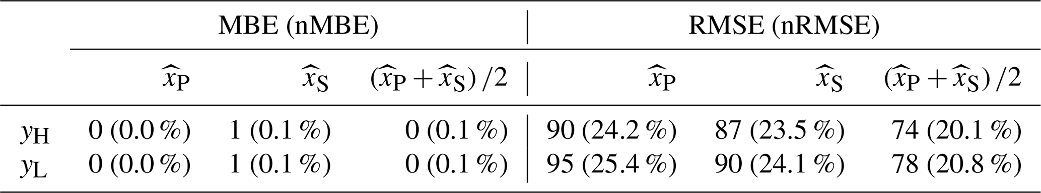
Table 1 shows the overall bias and accuracy of the two satellite-retrieved products at the validation location. Both MBE and RMSE are presented in the same unit as GHI, which is W m⁻². Their relative counterparts, i.e., normalized MBE (nMBE) and normalized RMSE (nRMSE), prefixed with “n” and noted in parentheses, are normalized with respect to the mean instead of the maximum. Several interesting observations can already be made from Table 1.

Table 1 Measure-oriented validation results of x_P and x_S, with respect to y_H and y_L. Both MBE and RMSE are in W m⁻², with the normalized metrics noted in parentheses.

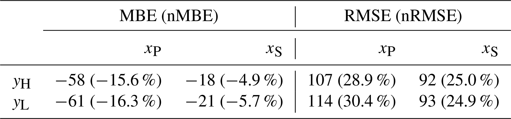
First, although all cases show negative MBEs, which suggests that both products underestimate GHI, the MBEs referenced to the high-accuracy ground-based observations are smaller than those referenced to the low-accuracy observations. This reveals that bias in observations propagates into the validation results. However, such an effect is directional, i.e., only if the bias of the observations and retrievals is of different signs will the apparent bias be larger than the true bias. Second, the differences in bias do not fully propagate into accuracy. The nMBE of x_S with respect to y_H and y_L are −18 and −21 W m⁻², respectively, but the difference between the RMSEs is smaller. This result can be explained through the bias–variance decomposition of MSE, in which bias only contributes partially to the overall accuracy. Third, the RMSEs of x_S evaluated against y_H and y_L are rather indistinguishable, which highlights the main deficiency of measure-oriented validation – the results are often ambiguous and therefore misleading. More specifically, if RMSE is used as the sole performance measure, conclusions such as “y_H and y_L do not make a difference in validating x_S” may be yielded.

In any case, the present measure-oriented validation suggests the superiority of the statistically retrieved GHI over the physically retrieved ones. This is not surprising, for the quality of the physical irradiance retrieval algorithms depends highly on the quality of those atmospheric state inputs, such as aerosols or water vapor. However, the NSMC has yet to establish a mature retrieval system for FY-4B (Xia et al., 2025), and directly inputting the imprecise atmospheric states to the retrieval algorithm can lead to unphysical or unrealistic irradiance values, which demand further investigation. However, measure-oriented validation offers only an overview of the product quality but lacks diagnostic ability at large. To that end, distribution-oriented validation ought to be employed if one aims to analyze and improve product quality.

3.2 Overall results of distribution-oriented validation

As previewed in Sect. 2.3, distribution-oriented validation allows both visual and quantitative assessments of the joint distribution of retrieval (X) and observation (Y), which are both considered in the present context as random variables. Since the joint distribution f(x,y) can be factorized into f(x), f(y|x), f(y), and f(x|y) via Bayes' theorem, visual assessment is facilitated by plotting out the joint, marginal, and conditional densities. On the other hand, quantitative assessment under the distribution-oriented validation mainly revolves around the MSE decompositions, e.g., Eqs. (5)–(7), from which a comprehensive collection of aspects of retrieval product quality can be gauged.

3.2.1 Visual validation

Given two sets of irradiance retrievals, namely, x_P and x_S, alongside two sets of ground-based observations, namely, y_H and y_L, four groups of retrieval–observation pairs can be formed; they are, (x_P,y_H), (x_S,y_H), (x_P,y_L), and (x_S,y_L). Each of these combinations results in a set of joint, marginal, and conditional densities, which are depicted in Figs. 4–6.

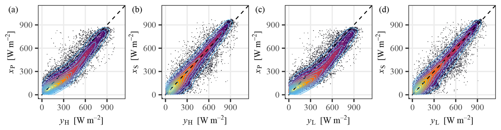
Figure 4 The joint PDFs of retrievals and observations. Panels (a)–(d) correspond to the different combinations of x_P, x_S, y_H, and y_L. The contours show the 2D kernel densities.

The joint PDFs in Fig. 4 are represented through contour lines superimposed upon x–y scatter plots, in which brighter colors correspond to higher point density. The physical retrieval product manifests its most striking characteristic through systematic irradiance underestimation, producing a distinctly nonlinear relationship with both the high- and low-accuracy observations. In an ideal case, scatter points should cluster tightly about the identity line. However, neither the (x_P,y_H) and (x_P,y_L) distributions exhibit this desired behavior. The underestimation of x_P is rather systematic, as it occurs over almost the entire irradiance range from 100–1000 W m⁻², strongly suggesting an inherent algorithmic deficiency. Under normal circumstances, clear-sky conditions should yield highly accurate retrievals, resulting in dense point clusters along the identity line, as exemplified by the scatters in Fig. 4b and d. The observed deviation from this expected pattern in Fig. 4a and c leads us to hypothesize that the physical algorithm employed by NSMC has poor clear-sky irradiance retrieval ability, possibly due to the low and inconsistent quality of aerosol and water vapor, which serve as essential inputs for clear-sky irradiance computation. In fact, improving individual stages of the physical irradiance retrieval process has been identified as the foremost scientific challenge of the current FY-4B products (Xia et al., 2025).

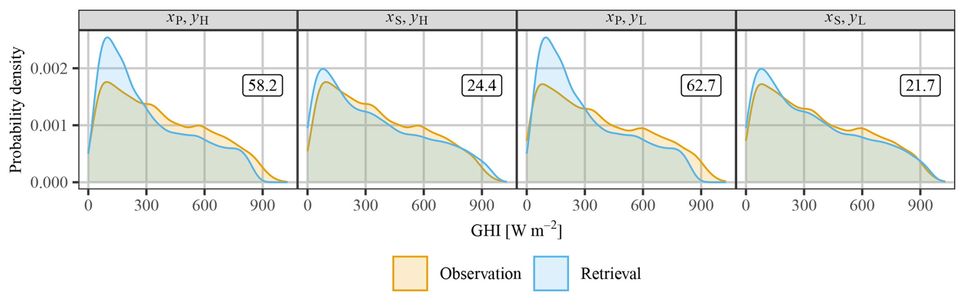
Figure 5 The marginal PDFs of retrievals (x_P or x_S) and observations (y_H or y_L). The number in the top-right corner of each subplot is the Wasserstein distance between the corresponding marginal densities.

Figure 5 shows the marginal densities of retrieval and observation, under the four combinations. The number in the top-right corner of each subplot indicates the Wasserstein distance between two PDFs, which gauges their similarity, the smaller the better. The disagreements between the physical retrievals with respect to both high- and low-accuracy observations are larger than those between the statistical retrievals and observations, which is consistent with the finding from Fig. 4. It can be seen that the PDF of x_P is higher in the low-irradiance range but lower in the high-irradiance range than the PDFs of the two sets of observations, again indicating underestimation. In contrast, the alignment between the PDFs of x_S and observations is much closer. But interestingly, in the case of x_S, the validation against y_L returns a lower Wasserstein distance than y_H, which signifies the potential danger of an overconfident validation when low-accuracy observations are used as reference.

Figure 6 The conditional PDFs of (a) observation given retrieval and (b) retrieval given observation, for different x_P, x_S, y_H, and y_L combinations. The colors indicate quantiles of the respective conditional PDF, with brighter ones being closer to the median.

Finally, we examine the conditional PDFs presented in Fig. 6, where the upper row displays f(y|x) and the lower row f(x∣y). The color gradations within these conditional distributions correspond to quantile values, whereas the black dots denote conditional means. It is a fundamental tenet of proper calibration that $\mathbb{E}\left(Y\right|X=x)=x$ must hold universally across all x. This calibration condition permits direct evaluation of both x_P and x_S through inspection of Fig. 6a, where each panel exhibits numerous distinct conditional distributions. The sequence of black dots represents $\mathbb{E}\left(Y\right|X=\mathrm{0}),\mathbb{E}(Y|X=\mathrm{100}),\mathrm{\dots },\mathbb{E}\left(Y\right|X=\mathrm{1000})$. Consequently, the proximity of these markers to the identity line provides a visual aid for assessing the calibration quality, i.e., the closer to the identity line the black dots are, the smaller the average deviation of $\mathbb{E}\left(Y\right|X=x)$ from x is, which in turn implies better calibration. Clearly then, x_P is less calibrated than x_S. In an analogous fashion, the quantity $\mathbb{E}\left(X\right|Y=y)=y$ can be assessed through Fig. 6b, in which the black dots correspond to $\mathbb{E}\left(X\right|Y=\mathrm{0}),\mathbb{E}(X|Y=\mathrm{100}),\mathrm{\dots },\mathbb{E}\left(X\right|Y=\mathrm{1000})$. It is evident that the conditional biases, i.e., $\mathbb{E}\left(X\right|Y=y)-y$, for $y=\mathrm{0},\mathrm{100},\mathrm{\dots },\mathrm{1000}$, are larger for x_P than for x_S, confirming the superiority of the latter. One should note that the deviations $\mathbb{E}\left(Y\right|X=x)-x$ and $\mathbb{E}\left(X\right|Y=y)-y$ are directional. Therefore, during quantitative evaluation, taking the absolute or squaring the term before averaging is necessary, as shown below. The final observation from Fig. 6 is that the conditional densities of x_P are often asymmetrical, which can be attributed to two possible reasons. First, the asymmetry may originate from misclassification of sky condition, e.g., due to the parallax effect, where a clear pixel is misidentified as cloudy. In other cases, the asymmetry may be simply the effect of poor-quality input to the retrieval algorithm.

3.2.2 Quantitative validation

Distribution-oriented validation also allows for quantitative assessment of various aspects of product quality. A total of six aspects of product quality, which are based on Eqs. (5)–(7), are considered herein. Given a set of validation samples, with X denoting the retrieval and Y the observation, the six aspects of quality are association, unconditional bias, calibration, resolution, type-2 conditional bias, and discrimination. They can be quantified through 𝙲𝚘𝚟(X,Y), [𝔼(X)−𝔼(Y)]², ${\mathbb{E}}_X[X-\mathbb{E}(Y\left|X\right){]}^{\mathrm{2}}$, ${\mathbb{E}}_X\left[\mathbb{E}\right(Y\left|X\right)-\mathbb{E}\left(Y\right){]}^{\mathrm{2}}$, ${\mathbb{E}}_Y[Y-\mathbb{E}(X\left|Y\right){]}^{\mathrm{2}}$, and ${\mathbb{E}}_Y\left[\mathbb{E}\right(X\left|Y\right)-\mathbb{E}\left(X\right){]}^{\mathrm{2}}$, respectively. These aspects of product quality are summarized and defined in Table 2, alongside their relevance to the distribution-oriented validation.

Table 2 The definitions and relevance of different aspects of product quality to distribution-oriented validation (Murphy, 1993).

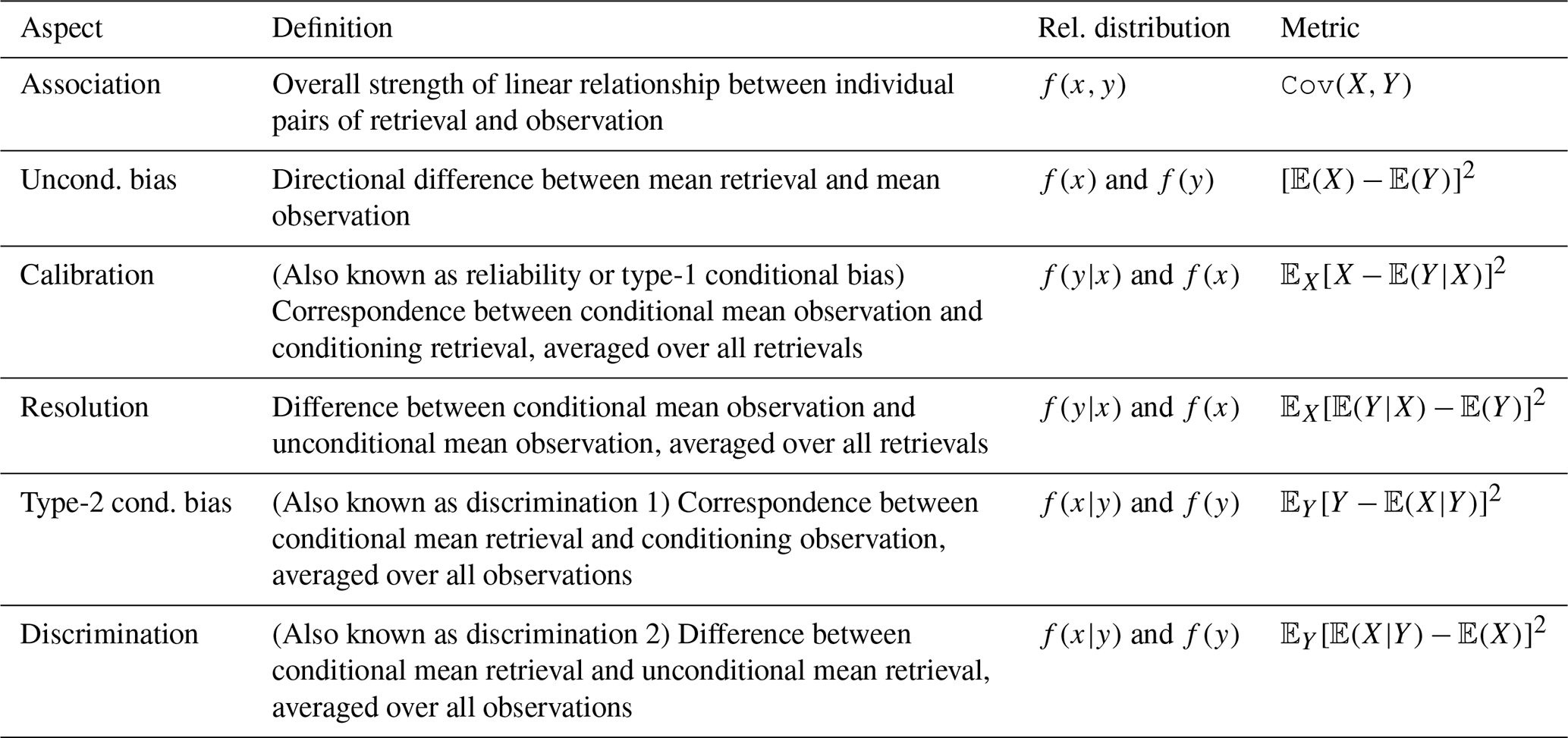
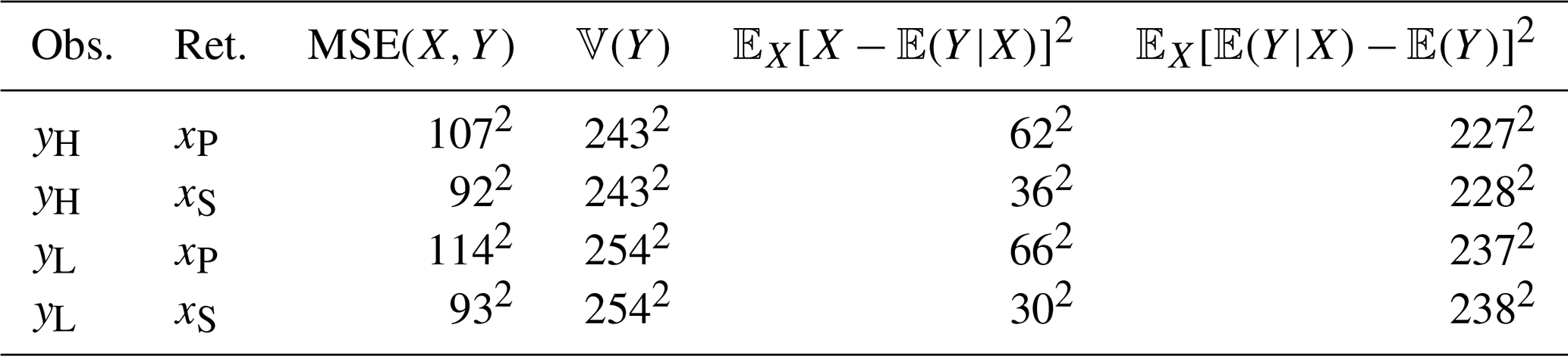
Table 3 Results of bias–variance decomposition of MSE, cf. Eq. (5), based on different combinations of x_P, x_S, y_H, and y_H. The metrics are written as exponentiations, such that all bases have the unit of W m⁻².

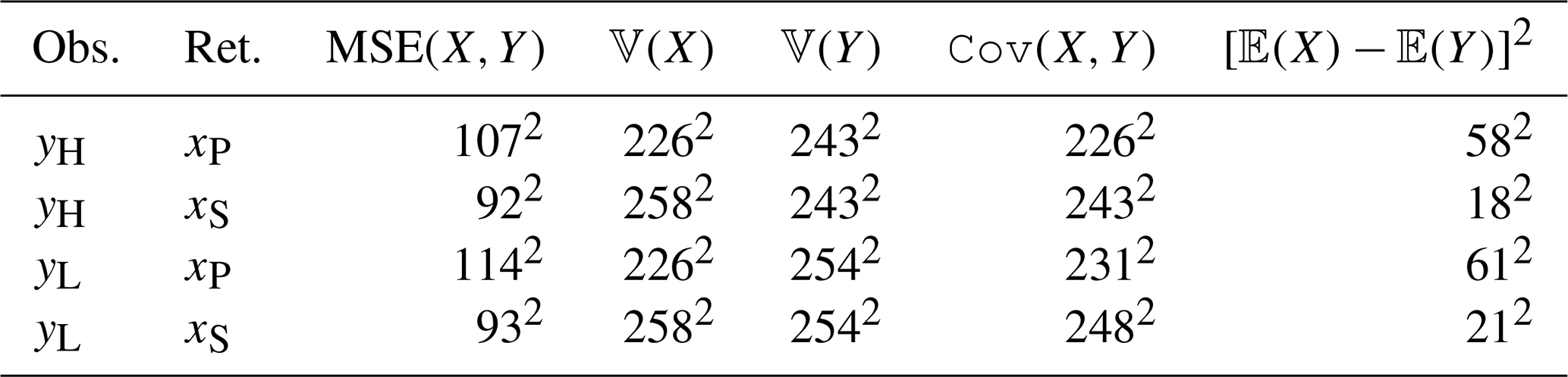
Table 3 lists the results of bias–variance decomposition of MSE, based on different combinations of x_P, x_S, y_H, and y_H. In terms of the variances, the standard deviation of y_H is 243 W m⁻², and compared to that, y_L is overdispersed with a standard deviation of 254 W m⁻². As for the retrievals, x_S is even more overdispersed, whereas x_P is underdispersed. On this point, the variance of x_S is closer to that of y_L and the variance of x_P is closer to that of y_S, which implies that y_L exaggerates the performance of x_S but understates that of x_P. In terms of association, i.e., the 𝙲𝚘𝚟(X,Y) column, the highest value (248² W² m⁻⁴) is seen when the statistical retrievals are validated using low-accuracy observations, whereas the lowest value (226² W² m⁻⁴) is seen when the physical retrievals are validated using high-accuracy observations. For both physical and statistical retrievals, the results are consistent – the low-accuracy observations tend to yield overconfident results by exaggerating the association. In terms of the unconditional bias, i.e., the [𝔼(X)−𝔼(Y)]² column, the opposite is true, in that, the low-accuracy observations return larger biases, announcing the products worse than they actually are, by about 3 W m⁻², which is quite significant when considering it in the light of currently available high accuracy satellite-retrieved irradiance datasets (Yang and Bright, 2020). Overall, Table 3 strongly evidences that low-accuracy observations should not be used to validate gridded irradiance.

Table 4 Same as Table 3, but for calibration–refinement decomposition of MSE, cf. Eq. (6).

Moving on to Table 4, which shows the results of calibration–refinement decomposition of MSE, more interesting insights can be gained. First, the physically retrieved product is less calibrated than the statistical one, which agrees with the earlier visual assessment. Recall that for two sets of retrievals, the one with a smaller value of calibration should be preferred. On this point, the calibration terms corresponding to x_P – see the ${\mathbb{E}}_X[X-\mathbb{E}(Y\left|X\right){]}^{\mathrm{2}}$ column – are higher than those of x_S, rendering x_P inferior. In terms of resolution, i.e., the ${\mathbb{E}}_X\left[\mathbb{E}\right(Y\left|X\right)-\mathbb{E}\left(Y\right){]}^{\mathrm{2}}$ column, the choice of observations appears to have a larger impact on the validation results than the products themselves, which is a bit surprising. The resolutions of both x_P and x_S are ∼227² W² m⁻⁴ when evaluated against y_H, and are about ∼237² W² m⁻⁴ when evaluated against y_L. Since for a given set of observations, 𝔼(Y) takes a fixed value, the similarity must be attributed to 𝔼(Y|X), and one can conclude that the resolving power of x_P and x_S are comparable.

Table 5 Same as Table 3, but for likelihood–base rate decomposition of MSE, cf. Eq. (7).

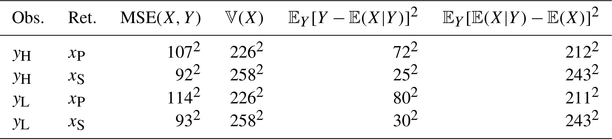
For the likelihood–base rate decomposition of MSE, its results are tabulated in Table 5. In terms of the type-2 conditional bias, the statistically retrieved product again shows superiority, regardless of whether the high- or low-accuracy observations are used for validation. It is worth noting that the type-2 conditional bias of x_S appears higher when validated using y_L than using y_H, which contrasts the former case, where the calibration (i.e., type-1 conditional bias) of x_S appears higher when validated using y_H than using y_L. As for discrimination, the difference in validation results across products is now larger than the difference across observation choices, which also contradicts the finding from Table 4.

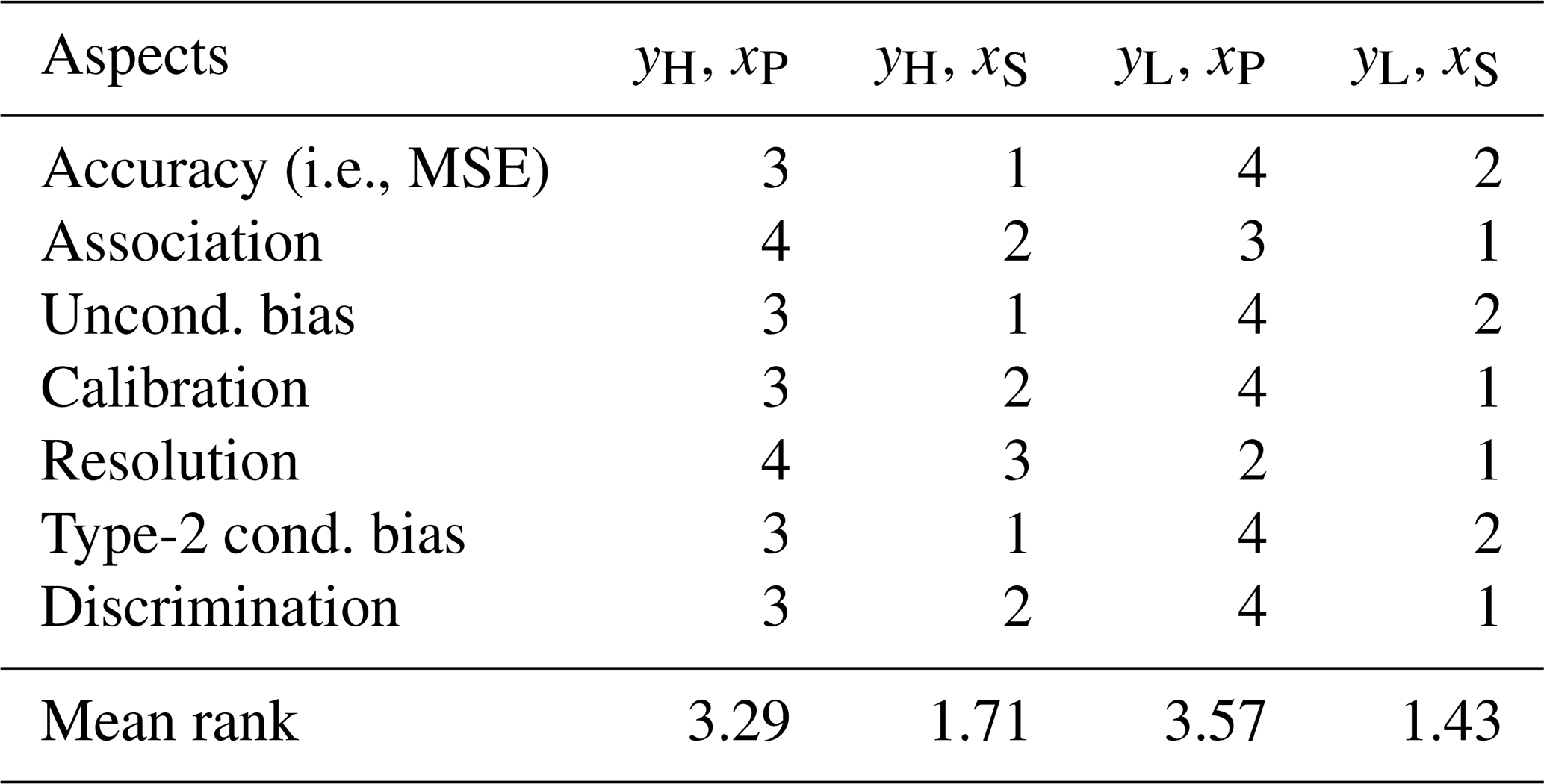
To give a summary of the quantitative assessment, a linear ranking method (see Alvo and Yu, 2014) is applied to the above results. There are four combinations of x_P, x_S, y_H, and y_H, and the mean rank of the ith combination, denoted by m_i, is:

$$\begin{array}{}\text{(8)}& m_i=\sum _{j=\mathrm{1}}^{\mathrm{4}\mathrm{!}}{\displaystyle \frac{n_j{v}_j\left(i\right)}{n}},\end{array}$$

where v_j with $j=\mathrm{1},\mathrm{2},\mathrm{\dots },\mathrm{4}\mathrm{!}$ represent all possible rankings of the four combinations, n_j is the frequency of occurrence of these rankings, $n=\sum n_j$ is the total number of ranking exercises, and v_j(i) denotes the score of the ith combination in ranking j. Table 6 shows the ranking of different combinations, together with their mean ranks computed using Eq. (8). It can be seen that there are four rankings, namely, $v_{\mathrm{1}}\left(i\right)=(\mathrm{3},\mathrm{1},\mathrm{4},\mathrm{2})$, $v_{\mathrm{2}}\left(i\right)=(\mathrm{4},\mathrm{2},\mathrm{3},\mathrm{1})$, $v_{\mathrm{3}}\left(i\right)=(\mathrm{3},\mathrm{2},\mathrm{4},\mathrm{1})$, and $v_{\mathrm{4}}\left(i\right)=(\mathrm{4},\mathrm{3},\mathrm{2},\mathrm{1})$, and the corresponding n_j's are 3, 1, 2, and 1, respectively. The foremost finding is that the rankings based on various quantification metrics are not unified, which again highlights the pitfall of measure-oriented validation. Next, the statistically retrieved irradiance, in this case, has low mean ranks and thus outperforms the physically retrieved ones, which is to be further investigated below. Last but not least, when low-accuracy observations are used to validate satellite-retrieved products, it can offset the results in both directions – i.e., y_L exaggerates the performance of x_S (y_L results in a lower mean rank of 1.43 than the 1.71 of y_H) but understates that of x_P (y_L results in a higher mean rank of 3.57 than the 3.29 of y_H) – which is not desirable in any case. Before we end this section, it is worth mentioning that variance plays an important role in validation. The variance ratio between observation and retrieval is further linked to calibration, type-2 conditional bias, and discrimination. Interested readers are referred to Mayer and Yang (2023) for further reading.

Table 6 Ranking of validation results in terms of different aspects of product quality.

3.3 Validation of hourly and daily averages

Among the various factors that influence the quality of satellite-retrieved irradiance, the three-dimensional (3D) effects of clouds, including the parallax effect, arguably constitute the most significant source of error. This phenomenon manifests when cloud presence in either the sun-to-surface path or the surface-to-satellite path fails to coincide, leading to erroneous sky condition identification (Huang et al., 2019). Such misidentification poses substantial contamination risks to retrieval accuracy and thus validation outcomes, prompting some researchers to advocate for the exclusion of retrieval–observation pairs exhibiting differences exceeding three standard deviations from the mean (Wang and Pinker, 2009). An alternative approach is based on the well-documented fact that the 3D effect of clouds rapidly decreases as the temporal resolution of retrieval gets coarse (Huang et al., 2016). This has led to widespread adoption of hourly and daily product validation in the literature (e.g., Shi et al., 2023; Huang et al., 2023). In accordance with this methodological convention, we have aggregated the original 15 min data into both hourly and daily resolutions in this section, with sample numbers of 3740 and 355, respectively.

Table 7 Same as Table 1, but for hourly and daily samples.

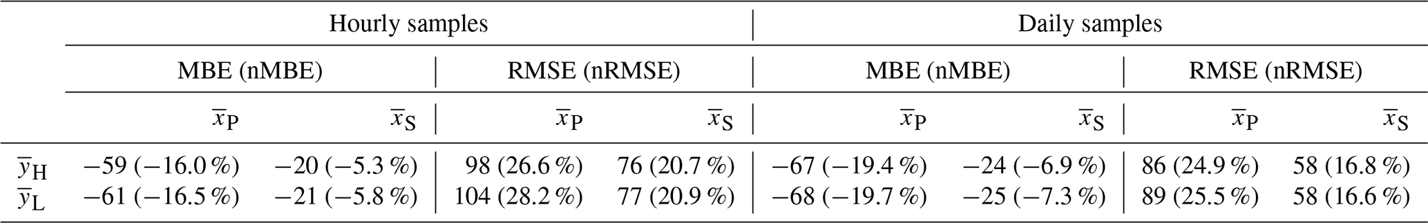
In accordance with the presentation style of Table 1, the overall biases and accuracies of hourly and daily samples are listed in Table 7. Comparing these tables reveals that the accuracy improves as the temporal resolution of the samples decreases. In contrast, the bias becomes larger after averaging. Particularly for daily samples, the bias of x_P shoots over −19 %, unequivocally demonstrating fundamental algorithmic deficiencies, which motivate site-specific bias correction. That said, given that aggregation should normally not affect bias, the differences between the 15 min and daily MBE come from the fact that days are shorter in winter – i.e., the proportion of the 15 min winter samples is lower than the proportion of the daily winter samples. The fact that the MBE decreased to a higher underestimation for the daily mean GHI in itself shows that the underestimation is higher in winter than in summer, which is shown in more detail in a later section.

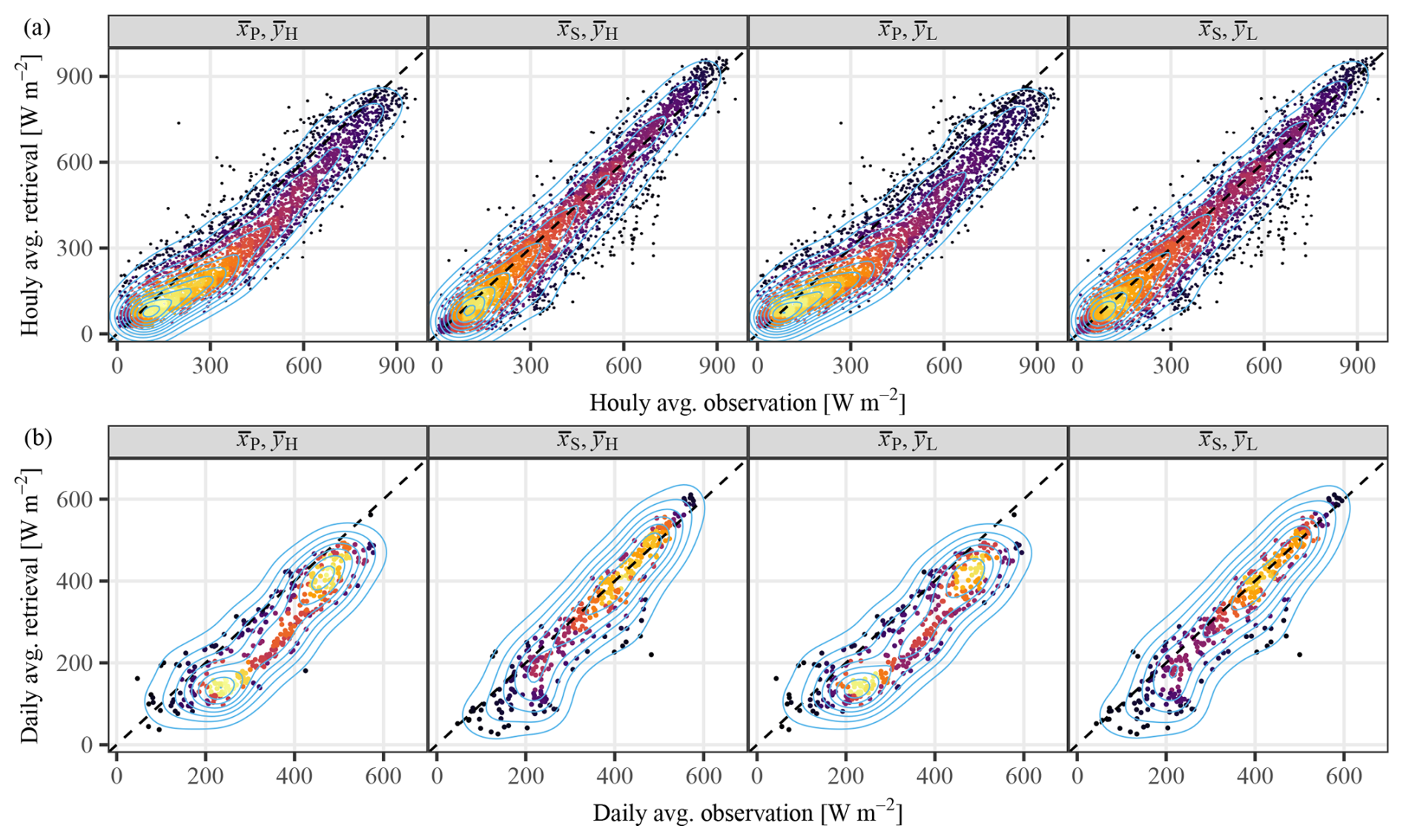
Figure 7 The joint PDFs of (a) hourly averages and (b) daily averages of retrievals and observations.

Figure 7 shows the joint PDFs of hourly and daily samples, under different combinations of ${\stackrel{\mathrm{‾}}{x}}_{\mathrm{P}}$, ${\stackrel{\mathrm{‾}}{x}}_{\mathrm{S}}$, ${\stackrel{\mathrm{‾}}{y}}_{\mathrm{H}}$, and ${\stackrel{\mathrm{‾}}{y}}_{\mathrm{L}}$, with bars annotating averages. The joint PDFs of the hourly samples exhibit notable consistency with those of the 15 min samples from Fig. 4, e.g., the consistent underestimation and nonlinearity in ${\stackrel{\mathrm{‾}}{x}}_{\mathrm{P}}$ seen earlier are again visible. The joint PDFs of the daily samples reveal a pronounced density peak near 450 W m⁻², indicative of prevailing clear-sky conditions at the validation location. Of particular concern is that the scatter of the daily samples of ${\stackrel{\mathrm{‾}}{x}}_{\mathrm{S}}$ only packs very loosely around the identity line, especially over the low irradiance range of 100–300 W m⁻², which contradicts earlier reports of similar Fengyun irradiance products, cf. Fig. 5 in Huang et al. (2023) and Fig. 5 in Shi et al. (2023). This discrepancy potentially suggests the influence of winter snow cover on retrieval accuracy within the Dwa Köppen climate regime, which is to be further examined in Sect. 3.5.

3.4 Validation results after bias correction

Within the domain of solar energy meteorology, the imperative for bias correction in satellite-retrieved irradiance arises from a fundamental economic consideration: The precision of mean irradiance estimates bears direct consequence upon the financial viability and projected returns of solar energy projects (Yang et al., 2022b). This location-specific bias correction procedure is better known as site adaptation, which has attracted much research effort in the past decade (e.g., Zainali et al., 2024; Yang and Gueymard, 2021; Polo et al., 2016). Among various statistical and machine learning site-adaptation methods, quantile mapping stands as a classic option. More importantly, quantile mapping is more amenable than linear regression when nonlinearity is present in the data, such as the case of x_P. Mathematically, quantile mapping is simply

$$\begin{array}{}\text{(9)}& \widehat{x}={\widehat{F}}_Y^{-\mathrm{1}}\left[{\widehat{F}}_X\left(x\right)\right],\end{array}$$

where ${\widehat{F}}_Y(\cdot )$ and ${\widehat{F}}_X(\cdot )$ are empirical cumulative distribution functions (ECDFs) of observation and retrieval, respectively; ${\widehat{F}}_Y^{-\mathrm{1}}(\cdot )$ is the inverse function of ${\widehat{F}}_Y(\cdot )$, also known as the quantile function; x is an arbitrary retrieval value; and $\widehat{x}$ is the corrected value.

Table 8 Same as Table 1, but for the bias-corrected x_P and x_S after quantile mapping, which are denoted as ${\widehat{x}}_{\mathrm{P}}$ and ${\widehat{x}}_{\mathrm{S}}$. Additionally, the results of a simple combination of ${\widehat{x}}_{\mathrm{P}}$ and ${\widehat{x}}_{\mathrm{S}}$ are shown in the $({\widehat{x}}_{\mathrm{P}}+{\widehat{x}}_{\mathrm{S}})/\mathrm{2}$ columns, demonstrating the complementarity of the two products.

Certainly, ${\widehat{F}}_Y(\cdot )$ and ${\widehat{F}}_X(\cdot )$ need to be trained before applying quantile mapping to new data points. To that end, the 15 min samples are randomly split into two groups, namely, A and B. After the samples in B are quantile mapped using the ${\widehat{F}}_Y(\cdot )$ and ${\widehat{F}}_X(\cdot )$ trained using A, the two groups switch, such that the bias-corrected versions of x_P and x_S has the same number of samples as the original data. The updated MBEs and RMSEs are provided in Table 8. It can be seen that the bias has been effectively eliminated, and thus translated to improved accuracy, in all cases. We further test the effect of combining the physical and statistical products by taking the arithmetic mean of the two time series, which is a fairly common strategy in forecasting science, leveraging the “wisdom of the crowd” (Wang et al., 2023; Atiya, 2020). A substantial reduction in RMSE is observed, which implies the complementarity of the two products. Nonetheless, despite that the bias-corrected samples have no bias with respect to both y_H and y_L, the RMSEs against y_L are higher across the board, indicating that using low-accuracy observations as reference during validation may return underconfident results, by about 0.8 % in this particular case.

3.5 Noticeable algorithmic limitations during winter

Hitherto, our validation has proceeded through comprehensive analyses of all available samples. While these aggregate results adequately characterize the general performance attributes of both products, they necessarily obscure certain extreme cases where algorithmic performance degrades substantially. A more penetrating examination of these specific conditions promises to reveal important limitations in the underlying retrieval algorithms that might otherwise escape notice. For instance, all of those severely underestimated daily samples of ${\stackrel{\mathrm{‾}}{x}}_{\mathrm{S}}$ in Fig. 7b, with ${\stackrel{\mathrm{‾}}{x}}_{\mathrm{S}}-{\stackrel{\mathrm{‾}}{y}}_{\mathrm{H}}<-\mathrm{80}$ W m⁻², come from winter months, which indicates a potential algorithmic limitation of Heliosat-2 during winter, with prolonged snow cover being typical over November to March for the Dwa climate.

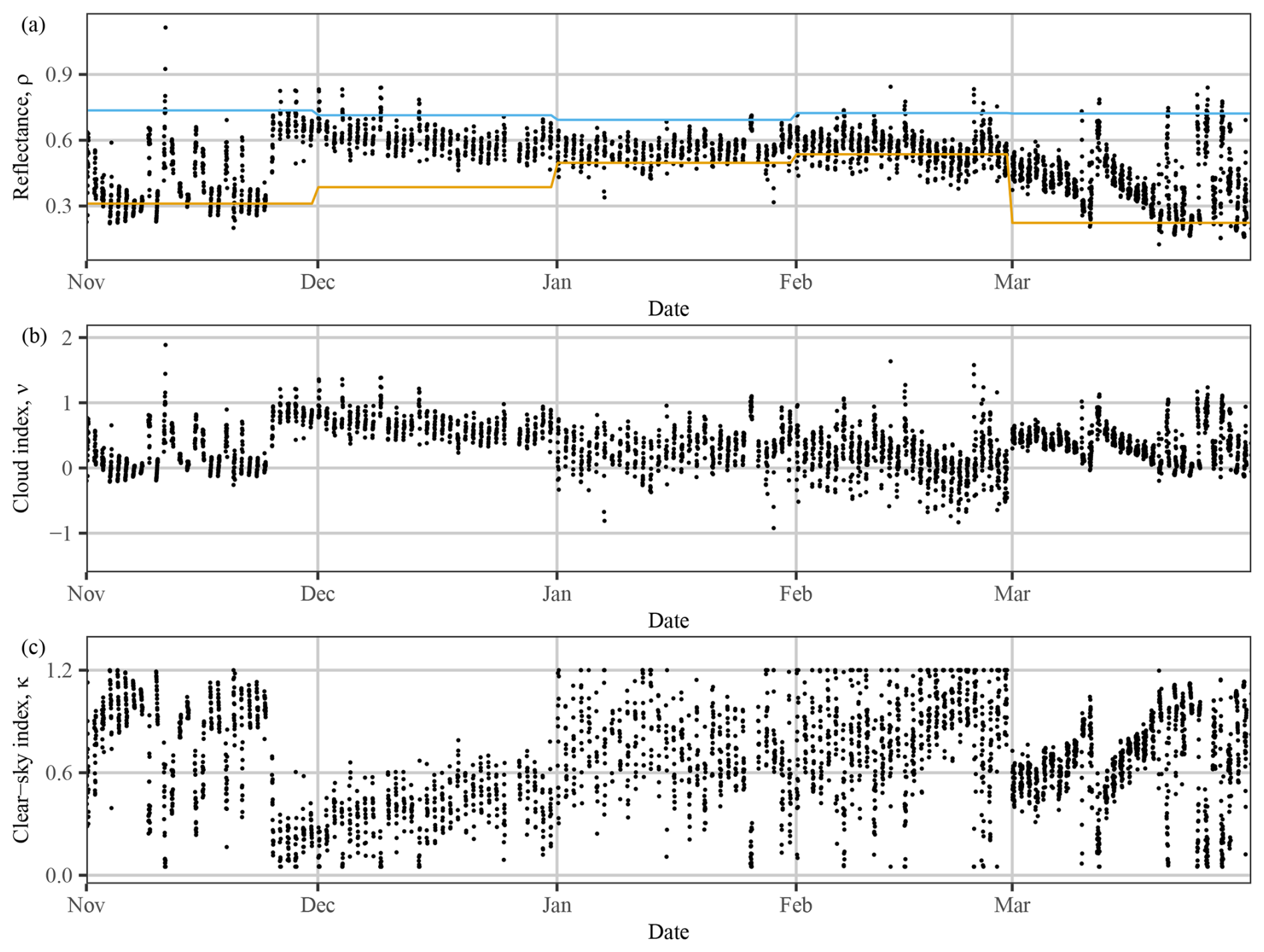
Figure 8 (a) Observed reflectance from the 0.65 µm visible channel of AGRI onboard FY-4B (black dots) and dynamic range (colored lines) from November 2024 to March 2025, with the corresponding (b) cloud index, ν, and (c) clear-sky index, κ.

The most transparent method for diagnosing temporal data lies in direct visual examination through time series plotting. In this regard, Fig. 8 shows the satellite-observed reflectance (ρ), the corresponding dynamic range (ρ_H and ρ_L), cloud index (ν), and clear-sky index (κ), over the winter months; the reader is referred to Appendix A for the relationship among these variables under the Heliosat-2 framework. Several insights are revealed. First, the satellite-observed reflectance exhibits an abrupt jump in late November and stays high until mid-March, which may be attributed to the long-lasting snow cover at the QIQ station. To verify this hypothesis, data from the United States National Ice Center's (NIC's) Interactive Multisensor Snow and Ice Mapping System (IMS) is considered. Figure 9a exemplifies the original data, which is in NetCDF format and polar stereographic projection. Figure 9b displays the time series of the IMS surface value at the QIQ station, over November and December 2024, which matches well with the elevated ρ time series, thus confirming the hypothesis.

Figure 9 (a) The NIC IMS map (in polar stereographic projection) of 24 November 2024, with the QIQ station marked with a white circle. (b) The time series of the IMS surface value at the QIQ station, from November 2024 to March 2025. (c) The scatter plot of x_S against y_H for all days with snow cover.

The next insight emerges from the monthly constant dynamic range employed by this version of the Heliosat-2 algorithm. In December, for instance, the lower bound ρ_L is underdetermined, resulting in overestimated ν and underestimated κ, as depicted in Fig. 8b and c. In contrast, ρ_L in February is overdetermined, resulting in numerous $\mathit{\nu }<-\mathrm{0.2}$ cases, which are unphysical. According to the Heliosat-2 computation, these cases would return κ=1.2, which is, again, extremely rare in reality. Overall, as evidenced by Fig. 9c, which plots the (x_S,y_H) scatter for all days with snow cover, the snow cover causes this version of the Heliosat-2 algorithm to severely underestimate the irradiance. Stated in another way, one may interpret this phenomenon as a case of cloud misidentification, in that, the algorithm is unable to distinguish the bright surface due to snow cover from clouds. To remedy this algorithmic pitfall, the bounds of dynamic range ought to be determined in a rolling fashion, which has been emphasized by Perez et al. (2002) in a very early publication. The difficulty, however, is one of computation – the iterative method for dynamic range determination for the full-disk area is too taxing, which promotes investigations into advanced sorting algorithms.

Figure 10 The time series plot of x_P and y_H in February 2025, alongside McClear GHI (G_hc).

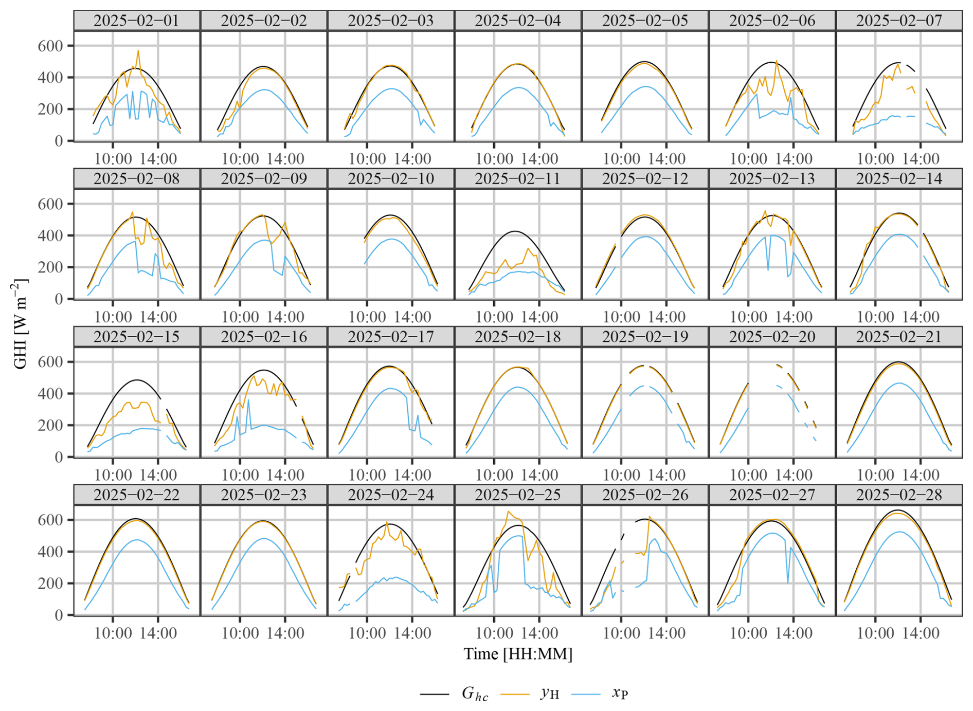
Whereas the algorithm limitations of the statistical product can be identified, the physical product is much more difficult to diagnose, given the complexity of the physical retrieval process. Therefore, only a simple visualization that reveals some product quality issues in winter is made, alongside a discussion on potential causes. Figure 10 shows the time series plot of x_P, y_H, and the McClear clear-sky irradiance in February 2025. Although the overall underestimation of the product is evident, it is fairly consistent throughout the month. From the plot of 8, 9, and 13 February, one may conclude that the product is able to capture the effect of clouds on irradiance to a good extent, resulting in ramp rates similar to the observations. Instead, it is the understimation of the clear-sky irradiance, see e.g., 4, 12, and 22 February, that affects the product quality. As clear-sky irradiance is primarily affected by the extraterrestrial irradiance, the sun–earth geometry, aerosols, and water vapors, with the former two being trivial to obtain, the underestimation is likely due to the imprecise information of the latter two, which echoes our earlier hypothesis in Sect. 3.2. This version of the NSMC's algorithm adopts an “indirect” approach that requires the AGRI observed channel reflectances as main inputs with little reliance on level-2 products, such as aerosol or water vapor. To that end, the inaccurate aerosol climatology used during retrieval might be the root cause of the systematic underestimation.

4 Conclusion

Validation of satellite-retrieved irradiance is ubiquitously performed in comparative studies concerning the quality of several products (e.g., Salazar et al., 2020; Marchand et al., 2018), as well as those studies investigating the change in radiation budget of the earth (e.g., Sanchez-Lorenzo et al., 2017; Zhang et al., 2015). With the validation results, various scientific assertions and conclusions are made. A critical yet frequently overlooked consideration concerns the reliability of observed inter-product variations or temporal radiation trends, which may be systematically distorted by the inherent limitations of the ground-based reference data employed in the validation process. To that end, this work formally investigates this issue by leveraging both high- and low-accuracy radiometric observations during the validation of two satellite-retrieved irradiance products for a location in a monsoon-influenced continental climate.

The contribution of this work is threefold. First, irradiance observations from a rarely reported climate regime (i.e., the Dwa Köppen climate) are presented, alongside two gridded irradiance products from the latest Chinese FY-4B weather satellite. Through rigorous analysis, we have identified a fundamental limitation in the operational physical retrieval algorithm implemented by NSMC: Its systematic underestimation of irradiance under clear-sky conditions reveals significant shortcomings in algorithmic maturity and implementation, particularly in terms of the quality of those atmospheric parameters intermediate to irradiance retrieval, such as aerosol optical depth or water vapor. Conversely, the statistical retrieval algorithm yields demonstrably superior results compared to the official NSMC product, at last for the geographical location under examination. However, the Heliosat-2 algorithm suffers substantial performance degradation under snow-covered conditions, in which the high surface albedo observed by the imager might be wrongfully attributed to clouds.

The second contribution resides in the novel application of the distribution-oriented validation framework, which was originally proposed to verify weather forecasts. Contrasting the measure-oriented validation, which is limited by the choice of those often confounding performance measures, the visual and quantitative assessments of the joint, marginal, and conditional distributions of retrieval and observation allow a more comprehensive understanding of various aspects of product quality, including bias, accuracy, association, calibration, resolution, and discrimination (cf. Tables 3–5). The main takeaway is that even if a certain product is validated to be strictly inferior in terms of bias and accuracy, it may still possess advantages in other aspects of quality (cf. Table 6). This complementarity between two or more products promotes combining or merging, as demonstrated in Table 8, which has led to a 4 % improvement in accuracy in this particular case.

Third, in regard to the quality of ground truth, the accumulated empirical evidence demonstrates conclusively that employing low-accuracy observations for irradiance retrieval validation introduces measurable deviations from what may be properly regarded as the “true”' values – that is to say, those values obtained through high-accuracy observational methods. Given the large sample size, these discrepancies represent actual differences in the validation outcomes rather than artifacts of measurement uncertainty. It must be highlighted that the deviations from the “true” value are not unidirectional, i.e., using the low-accuracy observations can yield both overconfident and underconfident results, depending on the particular metric under consideration. Moreover, the magnitude of the deviations caused by the low-accuracy observations is quite substantial, reaching several W m⁻² or a few percent. Indeed, numerous prior conclusions, such as the assertion that “satellite products overestimated radiation by approximately 10 W m⁻²” by Zhang et al. (2015), rest upon differentials of comparable scale. The present finding thus necessitates rigorous methodological caution: Any validation exercise employing low-accuracy observations must interpret apparent results with care, recognizing the substantial uncertainty introduced by the observational limitations themselves.

Appendix A: The Heliosat-2 algorithm

In a nutshell, the Heliosat-2 algorithm (Rigollier et al., 2004) first estimates the cloud index, ν, from the satellite-observed reflectance, and then converts it to the clear-sky index, κ, via

$$\begin{array}{}\text{(A1)}& \mathit{\kappa }=\left\{\begin{array}{ll}\mathrm{1.2},& \mathrm{if}\mathit{\nu }<-\mathrm{0.2}\\ a_{\mathrm{0}}+a_{\mathrm{1}}\mathit{\nu },& \mathrm{if}-\mathrm{0.2}\le \mathit{\nu }<\mathit{\alpha }\\ b_{\mathrm{0}}+b_{\mathrm{1}}\mathit{\nu }+b_{\mathrm{2}}{\mathit{\nu }}^{\mathrm{2}},& \mathrm{if}\mathit{\alpha }\le \mathit{\nu }<\mathrm{1.1}\\ \mathrm{0.05},& \mathrm{if}\mathrm{1.1}\le \mathit{\nu }\end{array}\right.\end{array}$$

where model parameters α=0.9, a₀=1.008, $a_{\mathrm{1}}=-\mathrm{0.96}$, b₀=2.8935, $b_{\mathrm{1}}=-\mathrm{5.1699}$, and b₂=2.3499 are determined empirically from data, in this case, observations from 38 ground-based stations in China (Huang et al., 2023). On the other hand, the determination of ν follows

$$\begin{array}{}\text{(A2)}& \mathit{\nu }={\displaystyle \frac{\mathit{\rho }-{\mathit{\rho }}_{\mathrm{L}}}{{\mathit{\rho }}_{\mathrm{H}}-{\mathit{\rho }}_{\mathrm{L}}}},\end{array}$$

where ρ is the satellite-observed reflectance after sun-to-surface and surface-to-satellite geometric corrections; ρ_L and ρ_H are the lower and upper bounds of the dynamic range derived from an adequate collection of ρ values, e.g., over a time period or over an area, see below. Physically, ρ_L corresponds to the expected clear-sky reflectance, whereas ρ_H corresponds to the expected reflectance of the brightest clouds.

In this version of the Heliosat-2 algorithm, ρ_H is first determined. More specifically, for each month, all samples of ρ with a zenith angle Z<80°, over China, are gathered and sorted; the 95 % quantile is then set as ρ_H. In other words, the ρ_H value for all of China is the same for a given month. In contrast, the determination of ρ_L is pixel-specific, and an iterative algorithm is used. Denoting the sorted samples of ρ from a specific pixel and a specific month with Z<75° as ρ_i, with $i=\mathrm{1},\mathrm{2},\mathrm{\dots },n^{\left(\mathrm{0}\right)}$, a threshold t⁽¹⁾ is obtained via

$$\begin{array}{}\text{(A3)}& t^{\left(\mathrm{1}\right)}=\sum _{i=\mathrm{1}}^{n^{\left(\mathrm{0}\right)}}{\mathit{\rho }}_i+\mathrm{0.035}{\mathit{\rho }}_{\mathrm{H}}.\end{array}$$

Subsequently, all ρ_i's that exceed threshold t⁽¹⁾ are removed, which results in n⁽¹⁾ remaining samples. In the second iteration, one proceeds with calculating

$$\begin{array}{}\text{(A4)}& t^{\left(\mathrm{2}\right)}=\sum _{i=\mathrm{1}}^{n^{\left(\mathrm{1}\right)}}{\mathit{\rho }}_i+\mathrm{0.035}{\mathit{\rho }}_{\mathrm{H}},\end{array}$$

and ρ_i's that exceed threshold t⁽²⁾ are removed. This iteration terminates when all remaining samples of ρ_i are below the threshold, and their average is used as ρ_L.

Appendix B: The computation of expectations in Eqs. (6) and (7)

The expectation terms in Eqs. (6) and (7) are not straightforward to compute, for they involve the estimation of the conditional means over the support, i.e., all possible x values with f(x)>0. In this work, the kernel conditional density estimation (KCDE) is used to estimate 𝔼(Y|X) and 𝔼(X|Y). Denoting the conditional distribution of observation given retrieval as f(y|x), its kernel conditional density estimator is

$$\begin{array}{}\text{(B1)}& \widehat{f}\left(y\right|x)=\sum _{i=\mathrm{1}}^n{w}_i(x)\cdot {\displaystyle \frac{\mathrm{1}}{h_y}}K\left({\displaystyle \frac{y-y_i}{h_y}}\right),\end{array}$$

where K(⋅) is the kernel function of choice, h_y is the unknown bandwidth of the kernel, and w_i(x) is given by

$$\begin{array}{}\text{(B2)}& w_i\left(x\right)={\displaystyle \frac{K\left(\frac{x-x_i}{h_x}\right)}{{\sum }_{i=\mathrm{1}}^{n}K\left(\frac{x-x_i}{h_x}\right)}},\end{array}$$

where h_x is another unknown bandwidth. Following Hyndman et al. (1996), the conditional mean estimator at arbitrary x₀ is

$$\begin{array}{}\text{(B3)}& \widehat{\mathbb{E}}\left(Y\right|X=x_{\mathrm{0}})=\sum _{i=\mathrm{1}}^n{w}_i(x_{\mathrm{0}})y_i.\end{array}$$

In this work, the Gaussian kernel is used without loss of generality, and h_x and h_y are both set to 10, following some empirical trial-and-error. Once $\widehat{\mathbb{E}}\left(Y\right|X=x_i)$ is computed for all x_i's, ${\mathbb{E}}_X[X-\mathbb{E}(Y\left|X\right){]}^{\mathrm{2}}$ can be computed via

$$\begin{array}{}\text{(B4)}& {\displaystyle \frac{\mathrm{1}}{n}}\sum _{i=\mathrm{1}}^n{\left[x_i-\widehat{\mathbb{E}}\left(Y\right|X=x_i)\right]}^{\mathrm{2}}.\end{array}$$

The other expectations can be computed in a similar fashion.