Water vapor content retrieval under cloudy sky conditions from SWIR satellite measurements in the context of C³IEL space mission project

A retrieval algorithm of integrated water vapor content above cloud, using shortwave infrared observations, is developed and evaluated through idealized and realistic atmospheric profiles, with its application currently limited to oceanic regions and latitudes within ±60°. Water vapor plays a crucial role in cloud formation and development, particularly in the formation of clouds resulting from convective processes. The resulting convective cloud locally influences the spatio-temporal variability of atmospheric water vapor content, through exchanges between cloud and its immediate environment. Therefore, a better understanding of the water vapor content above and around clouds is necessary to improve our comprehension of interactions between water vapor and cloud to better constrain Large-Eddy Simulations and numerical weather forecasting models. The algorithm was developed for the Cluster for Cloud evolution, ClImatE and Lightning space mission project. This mission, scheduled for 2028, aims to enhance our knowledge of the 3D convective cloud development velocities, the electrical activity associated with convective systems, and the water vapor content above and around the cloud. The retrieval algorithm presented in this study uses a Bayesian probabilistic approach, the optimal estimation method. The atmosphere is assumed to be composed of homogeneous plane-parallel layers, and synthetic radiance datasets were generated to test the developed retrieval algorithm. The feasibility of retrieving the integrated water vapor content above the cloud over the ocean from shortwave infrared radiances is shown to have, under idealized vertically homogeneous cloud profiles, absolute errors less than 2 kg m⁻² for optically thick clouds or when the integrated water vapor content is below 20 kg m⁻² and less than 1 kg m⁻² for very thick clouds with an optical thickness exceeding 150. Tests using realistic water vapor and cloud extinction profiles that present non-homogeneous vertical distributions show that integrated water vapor content above water type clouds could be retrieved with a Root-Mean-Square Error related to cloud vertical penetration of approximately less than 1 kg m⁻² except for optically thin and low-level clouds (cloud optical thickness less than 50 and cloud top height less than 2 km). For very low water vapor content encountered in the presence of high deep convective clouds, the retrieval algorithm tends to systematically overestimate the retrieved water vapor content due to an overestimation of the cloud extinction profile in the upper part of the cloud in the inversion model.

1 Introduction

Clouds play a significant role in Earth's energy balance, as they can induce a positive or negative radiative forcing whose uncertainty is still important (e.g., Stocker et al., 2013; Masson-Delmotte et al., 2021). Depending on their latitude, characteristics, altitude and temperature, their radiative forcing can be different (e.g., Ramanathan et al., 1989; Harrison et al., 1990). In fact, lower tropospheric clouds, which are composed primarily of liquid water, tend to reflect solar radiation at all wavelengths, resulting in a cooling effect (e.g., Fermepin and Bony, 2014), named the parasol effect (e.g., Crutzen and Ramanathan, 2003). In contrast, solar radiation goes through upper thin tropospheric clouds, such as cirrus but these thin high clouds absorb thermal radiation from the Earth and re-emit infrared radiation towards space at a lower temperature due to their cold temperature, thereby enhancing the greenhouse effect (e.g., Jensen et al., 1996; McFarquhar et al., 2000; Lee et al., 2009; Schmidt et al., 2010). A more detailed description of cirrus type clouds and their effects on the Earth-Atmosphere system can be seen in Lynch (2002). Deep convective clouds combines both effect as they reflect a significant amount of incoming solar radiation back into space and emit infrared radiation at a low temperature due to the high level of their top. It is therefore essential to better understand cloud development in order to accurately assess their radiative impact on the Earth's energy balance. As an example, Bony et al. (2015) address the scientific community with several questions aimed at emphasizing the importance of a better understanding of the role of cloud feedbacks and convective organization on climate, as well as the factors that influence cloud formation.

Cloud formation and development depend on the amount of water vapor available in the atmosphere. Indeed, at a given temperature, saturation is reached when the water vapor partial pressure equals the saturation vapor pressure. Water vapor will then condense either on Cloud Condensation Nuclei (CCN) to form new cloud droplets or on Ice Nuclei (IN), to form new ice crystals. The latent heat released during water vapor condensation and cloud formation not only disturbs the thermal structure of the atmosphere (e.g., Trenberth and Smith, 2005; Schneider et al., 2010) but also fuels cloud development through a chain reaction.

In the free troposphere, humidity influences the dynamical development of clouds through entrainment and detrainment processes. Convection processes, in turn, contribute significantly to the redistribution of energy and water vapor in the atmosphere (e.g., Blyth, 1993). Humidity above and around clouds is therefore an essential parameter in the process of cloud development, particularly in the case of convective clouds.

Many spaceborne remote sensing instruments have been developed to retrieve water vapor across various spectral domains. Microwave sounders such as the Sounder for Probing Vertical Profiles of Humidity (SAPHIR) aboard the French-Indian satellite MEGHA-TROPIQUES (e.g., Desbois et al., 2007), or AMSU (the Advanced Microwave Sounding Unit) aboard the NOAA satellite, make it possible to conduct measurements at all weather conditions and provide either humidity profiles or information on total water vapor content at a spatial resolution of 12 km at nadir for SAPHIR (e.g., Rao et al., 2013), 48 km at nadir for AMSU-A, and 16 km for AMSU-B (e.g., Rosenkranz, 2001; Karbou et al., 2005). Humidity profile retrieval in clear sky conditions or above thick clouds are also performed by the Infrared Atmospheric Sounding Interferometer (IASI) instrument operating in the thermal infrared (TIR) with a spatial resolution of 8 km (e.g., Schlüssel and Goldberg, 2002; Hilton et al., 2012). These instruments give a vertical information on the water vapor content in the atmosphere but their limitation to study cloud and water vapor interactions lies in their low spatial resolutions and not contiguous pixels, which do not allow for precise examination of these interactions.

Near-Infrared (NIR) or Shortwave Infrared (SWIR) imagers allow to derive water vapor content at a better spatial resolution under clear sky conditions through the differential absorption method, either with airborne measurements (e.g., Bouffiès et al., 1997), or from spaceborne sensors such as the POLarization and Directionaly of Earth Reflectance instrument (POLDER: e.g., Vesperini et al., 1999), the Medium Resolution Imaging Spectrometer (MERIS: e.g., Bennartz and Fischer, 2001), the MODerate resolution Imaging Spectroradiometer (MODIS: e.g., Gao and Kaufman, 2003) or the Ocean and Land Colour Instrument (OLCI:  Preusker et al., 2021). All of these retrieval algorithms propose parameterizations that link the Total Column Water Vapor (TCWV), in kg m⁻², to the ratio of NIR or SWIR spectral bands within absorbing and non-absorbing channels. However, in cloudy sky conditions, these parameterizations are no longer sufficient as clouds interact with the measurements. Indeed, in this particular spectral domain, clouds are not transparent to radiation (as it is in the microwave domain). Moreover, as clouds do not act as a perfect reflector, radiation penetrates the cloud and gets scattered, effectively extending the radiation path through the atmosphere and consequently increasing absorption by water vapor or any other absorbing gas. Albert et al. (2001) demonstrates the feasibility of retrieving water vapor content above cloud in the SWIR domain, over various types of surface, and in the presence of low and optically thick clouds, applying the differential absorption method to simulations conducted in the context of the POLDER and MERIS instruments. They demonstrated with simulations that the absorption of solar radiation within a water vapor absorption band is influenced by the “radiation path”, modified by the presence of clouds. On one hand, multiple scattering increases the path length traveled by radiation, leading to higher absorption by water vapor and consequently, a higher retrieved water vapor content. On the other hand, the presence of clouds reduces or stops the influence of lower atmospheric layers, resulting in reduced overall absorption (Albert et al., 2001). They conclude that retrieving water vapor above cloud is feasible for high values of cloud optical thickness. By adjusting the path in their method and applying it to POLDER measurements, they report an average root mean square error (RMSE) of 1.8 kg m⁻² over ocean, as compared with radio-sounding data. (Vidot et al., 2009) conducted a feasibility study using an optimal estimation method within the framework of the Orbiting Carbon Observatory (OCO) sensor, quantifying various type of errors to demonstrate the potential for retrieving column-averaged carbon dioxide mixing ratios over liquid water clouds above the ocean. Similarly, (Schepers et al., 2016) used SWIR measurements from the Greenhouse Gas Observing Satellite (GOSAT) to simultaneously retrieve the total columns of methane and carbon dioxide above clouds, along with cloud properties.

In this study, the objective is to retrieve the integrated water vapor content above cloud using SWIR satellite observations with high spatial and temporal resolution over the ocean in the context of the the Cluster for Cloud evolution, ClImatE and Lightning (C³IEL) mission. The main advantage that can be exploited is the knowledge of the cloud top height retrieved with good accuracy thanks to the CLOUD radiometers (Dandini et al., 2022). Firstly, in Sect. 2, we provide an overview of the study's context, specifically the space mission project C³IEL that contextualizes our work. Then in Sect. 3, we discuss the method employed in the developed retrieval algorithm. Section 4 shows the sensitivity of the C³IEL water vapor channels to the integrated water vapor content above cloud (IWV_AC). In Sect. 5, the algorithm is tested first under idealized cloudy atmospheric conditions, then under realistic conditions. Finally, Sect. 6 summarizes the main findings and perspectives.

2 The C³IEL space mission project

The space mission project named as the Cluster for Cloud evolution, ClImatE and Lightning, C³IEL (Rosenfeld et al., 2022) started in 2016 through a partnership between the French space agency (CNES) and the Israeli Space Agency (ISA). The mission is under development and is scheduled to be launched at the end of 2028, with a minimum expected duration of two years that could be extended to three years. Its primary objective is to explore the dynamical development of convective clouds, including cumulus congestus and cumulonimbus clouds. This will be achieved by gathering data at high spatial and temporal resolutions. Indeed, the satellites will rotate to track the same scene for 200 s and capture a sequence of 11 acquisitions of two simultaneous observations. C³IEL consist of a pair of satellites operating in tandem, distanced by about 150 km following a sun-synchronous orbit at about 01:30 PM local time at the equator. The altitude of the orbit is expected to be between 600 and 700 km. The underlying measurement principle is represented in Fig. 1. The viewing angles for each satellite will be approximately ±50, −42, −32, −20, and −7° on each side of the observed scene. Additionally, the first satellite will include a −55° angle, while the second satellite will include a +55° angle. Between each sequence of acquisitions, the satellites will have to return to their initial attitude, which implies a limited number of 4 sequences per orbit. The latitudes of these observation sequences will be chosen according to climatology of convective clouds. This strategy of observations will provide (1) the 3D envelope of convective clouds and their vertical/horizontal development velocities (Dandini et al., 2022) using the visible imagers named CLOUD, measuring at 670 nm with a high spatial resolution (20 m at nadir), (2) the associated electrical activity generated by convective processes with the instruments Lightning Optical Imager and Photometers (LOIP) consisting in visible imagers measuring at 777 nm with a spatial resolution of 140 m at nadir and three photometers at 337, 391 and 777 nm and (3) the water vapor content above and around convective clouds using the three shortwave infrared (SWIR) imagers, with a spatial resolution of 125 m at nadir.

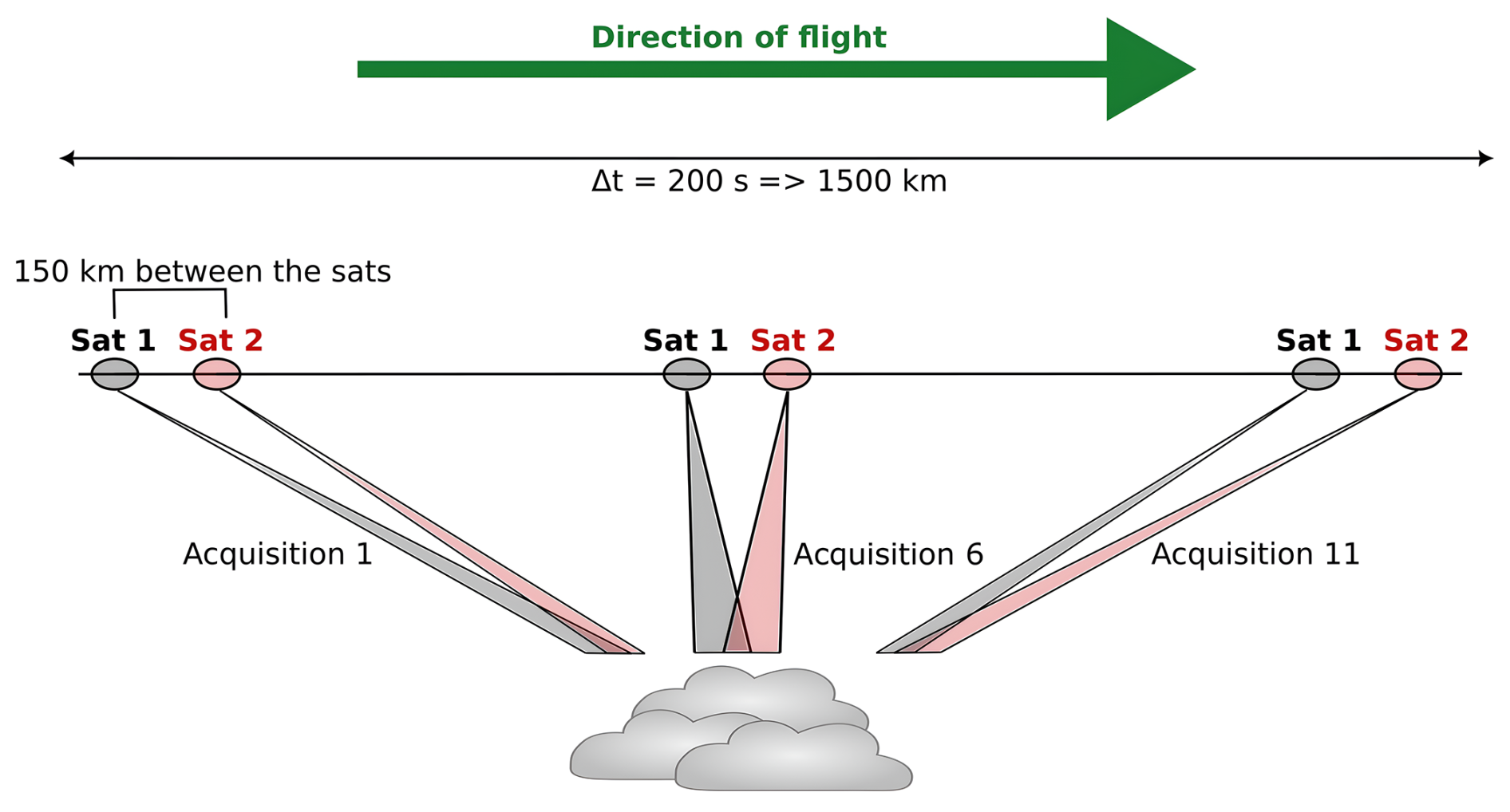
Figure 1 Illustration of the principle of the Cluster for Cloud evolution, ClImatE and Lightning (C³IEL) observations.

This paper focuses on the development of a retrieval algorithm for the integrated water vapor content above cloud (IWV_AC) from three SWIR water vapor imagers on each satellite. Figure 2 shows the water vapor transmission spectrum in this spectral range and the three spectral bands selected for the C³IEL water vapor imagers. The first band (1) is a non-absorbing band centered at 1.04 µm; the second band (2) is a moderately absorbing band centered at 1.13 µm; the third one is a highly absorbing band centered at 1.37 µm. These three bands have a spectral width of about 0.04 µm.

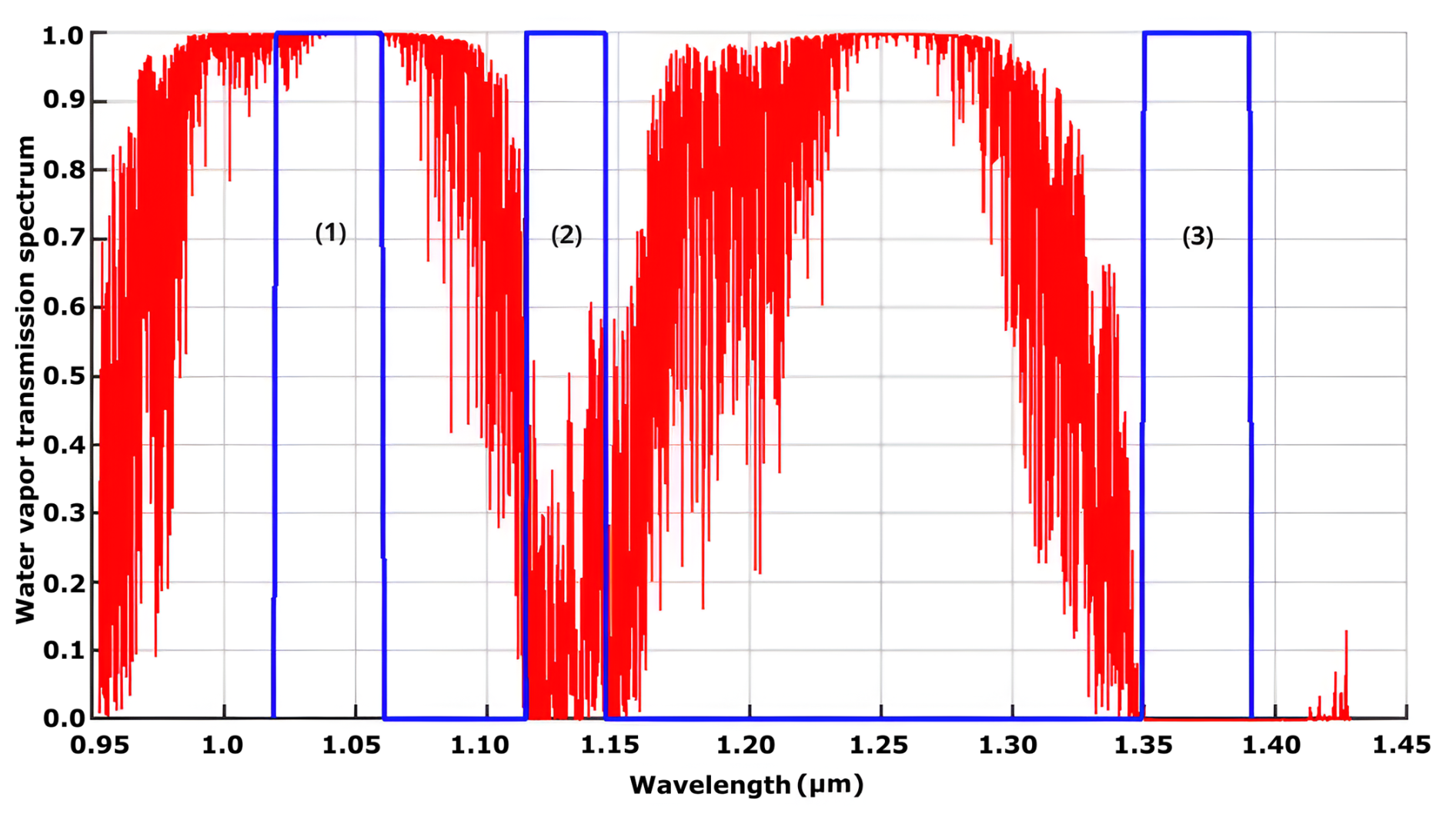
Figure 2 Water vapor transmission spectrum in clear sky condition at nadir (red curve) and the three SWIR spectral bands for the study of water vapor in the context of the C³IEL space mission (blue rectangles). Note that rectangular spectral response functions are used, as the actual SRF are not known.

3 Methodology

This section introduces the retrieval scheme used in our study. It follows an Optimal Estimation Method (OEM) scheme (Rodgers, 2000), with the aim to get the 1D equivalent cloud optical thickness (COT) and the integrated water vapor above cloud (IWV_AC). The OEM is a Bayesian statistical approach commonly used in remote sensing in order to estimate atmospheric and surface properties from measurements, such as satellite remote sensing (e.g., Sourdeval et al., 2013, 2015; Leonarski et al., 2020; Matar et al., 2023). The objective of the OEM is to minimize the difference between the measured and the simulated radiances, under the constraint of a priori knowledge about the atmosphere. Equation (1) formalizes how the OEM works:

$$\begin{array}{}\text{(1)}& \mathit{y}=F(\mathit{x},b)+\mathit{ϵ}\end{array}$$

where the vector y contains the measured radiances and F denotes the forward model including the model assumed for the retrieval and the radiative transfer code to get radiances from atmospheric properties. The state vector (x) contains the parameters to retrieve (see Sect. 3.1), whereas b specifies the fixed parameters within the forward model (see Sect. 3.2). Lastly, the vector ϵ contains the errors assumed to be randomly distributed, encompassing measurement uncertainties, errors in the fixed parameters and related to the forward model. Because forward model errors are extremely hard to estimate properly, as usually done only uncertainties associated with measurements and fixed parameters are considered in this paper.

3.1 Measurement and state vectors: y and x

Water vapor retrieval in the context of the C³IEL space mission is based on the exploitation of three spectral bands in the SWIR. The non-absorbing band (centered at 1.04 µm) is sensitive to the 1D equivalent cloud optical thickness (COT), representing the medium's reflectivity, while the two other bands (centered at 1.13 and 1.37 µm), which are also sensitive to the 1D equivalent COT, are used to retrieve the IWV_AC.

The measurement vector contains thus the radiance values measured in the three spectral bands described above:

$$\begin{array}{}\text{(2)}& \mathit{y}=\left[\begin{array}{c}{R}_{\mathrm{1.04}}\\ R_{\mathrm{1.13}}\\ R_{\mathrm{1.37}}\end{array}\right]\end{array}$$

As the C³IEL mission is still not in orbit, these radiances are simulated to develop and evaluate the algorithm using atmospheric and cloud profiles described in Sect. 5. Measurement vector data are associated with an uncertainty of 5 %. This value corresponds to the requirement on the accuracy of the radiance measured by the instrument (random error at 1σ), corresponding to random noise.

The state vector contains the desired parameters, the 1D equivalent COT and IWV_AC:

$$\begin{array}{}\text{(3)}& \mathit{x}=\left[\begin{array}{c}\text{1D COT}\\ {\text{IWV}}_{\mathrm{AC}}\end{array}\right]\end{array}$$

The uncertainty on the a priori knowledge is arbitrarily set to 10 000 %, in order to minimize its influence and give more weight to the measurements during the retrieval process.

At the end of the OEM process, the variance-covariance matrix of the retrieved state vector is computed and gives the uncertainties on the retrieved parameters (a posteriori uncertainties, noted σ_x) with the following relationship (Rodgers, 2000):

$$\begin{array}{}\text{(4)}& {\mathit{\sigma }}_x=\sqrt{{\left({\mathbf{S}}_{\mathrm{a}}^{-\mathrm{1}}+K_i^T{\mathbf{S}}_{\mathit{ϵ}}^{-\mathrm{1}}{K}_i\right)}^{-\mathrm{1}}}\end{array}$$

which is the square root of the a posteriori variance-covariance matrix. In this expression, S_a is the a priori variance-covariance matrix, K the jacobian, and S_ϵ the error variance-covariance matrix associated with the measurements and fixed parameters (see Appendix A for more details).

3.2 Fixed parameters: b

The cloud model defined in the developed retrieval algorithm assumes a 1D horizontally and vertically homogeneous plane-parallel layer between the cloud base height (noted Z_b) and its top altitude (noted Z_t), horizontally infinite over the ocean. Table 1 describes the fixed parameters used in the developed retrieval algorithm and their uncertainties.

Table 1 Description of the fixed parameters and their uncertainties.

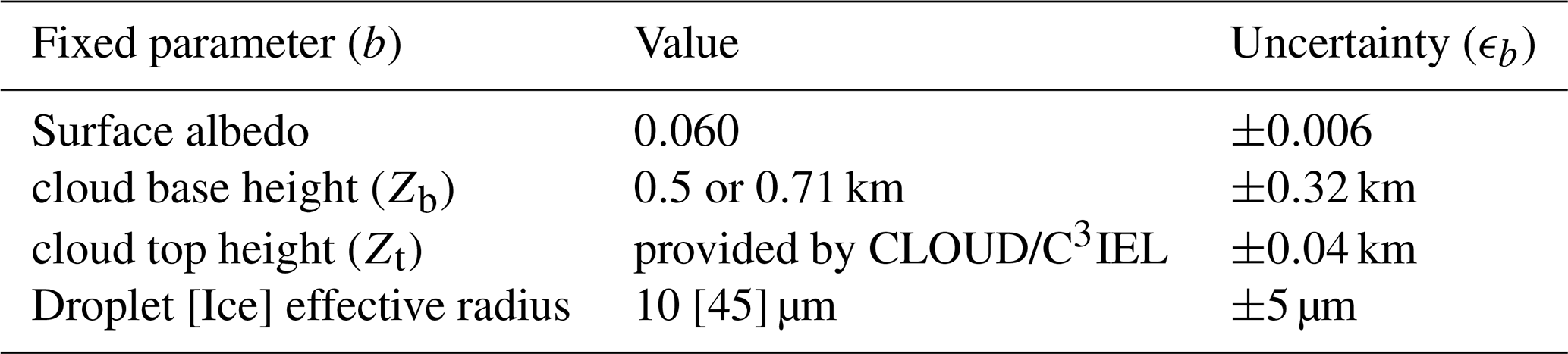
In this study, we consistently assign a surface albedo of 0.060, representing an ocean surface, with an uncertainty chosen to be 10 %. The cloud base height is set to 0.50 km for the idealized cases (Sect. 5.2.1) or 0.71 km for the realistic cases (Sect. 5.2) with an uncertainty of 0.32 km. These last two values represent the respective average and standard deviation values derived from the selected profiles (Eresmaa and McNally, 2014) for this study (Sect. 5.2.1). The cloud top height varies based on the atmospheric profile used to simulate the measurements. In practice, it will be determined by combining data from the pair of visible imagers designed for studying the 3D envelope and development velocities. The cloud top height uncertainty is set to 0.04 km (Dandini et al., 2022). For the idealized cases, the phase of the clouds is only liquid whereas for the realistic cases, for clouds with a top altitude above 4 km, we assume they consist of two distinct phases: a liquid phase between the cloud base height (Z_b) and Z=4 km, and an ice phase between Z=4 km and the cloud top height (Z_t). This fixed altitude of 4 km represents the average height of the 0 °C isotherm, according to the ECMWF profiles selected for this study. The effective radius of cloud droplets is fixed at an average value of 10 µm (e.g., King et al., 2004), with an accuracy of 50 %. The effective radius of ice crystals is set to an average value of 45 µm with an associated uncertainty of 5 µm. These values represent the average and standard deviation of the ice effective radius calculated using the Wyser parameterization (Wyser, 1998) applied on the whole database described in Sect. 5.2.1.

3.3 Radiative transfer model: F

Our study combined an Optimal Estimation Method with the radiative transfer code ARTDECO (Atmospheric Radiative Transfer Database for Earth and Climate Observation) in order to solve the Radiative Transfer Equation (RTE) by means of the adding-doubling model (de Haan et al., 1987). ARTDECO (https://www.icare.univ-lille.fr/artdeco/, last access: 28 November 2025) is a tool that gathers various models and data used to simulate Earth total and polarized atmosphere radiances and radiative fluxes, from the UV to the thermal IR range (200 to 50 µm). It uses the homogeneous plane-parallel approximation and allows to compute aerosols and clouds optical properties.

3.4 IWV_AC retrieval: principle and assumptions

Given the limited information on the atmospheric profile from the measurements, assumptions are made to constrain the model: molecular Rayleigh scattering is disregarded due to its negligible effect in the SWIR, and relative humidity (RH) is assumed to be 100 % within the cloud. For low- and mid-level clouds (Sect. 5.2.2), the assumption is applied with respect to liquid water. For high-level clouds (Sect. 5.2.3), relative humidity is defined as 100 % with respect to liquid water below 4 km and with respect to ice above.

As explained above, the main objective of the developed retrieval algorithm is to minimize the difference between the measured radiances and the radiances simulated by the forward model. The process begins with a first guess value for the state vector including the 1D equivalent cloud optical thickness (COT) and IWV_AC. For the COT, the first guess value is 10 and for the IWV_AC, the first guess value is calculated by integrating the SAS (Sub-Arctic Summer) water vapor profile from the cloud top altitude up to 20 km. In each iteration, the state vector is adjusted to achieve simulated radiances closer to the measured one. The COT, being an input parameter in the radiative transfer code, is subject to a direct adjustment at each iteration. The IWV_AC follows a different approach as it represents the vertical integration of the water vapor profile above clouds used in the forward model. The adjustment consists in applying, at each iteration, a multiplicative factor β to the water vapor profile, noted WV(z), from the cloud top height (Z_t) to the top of atmosphere. The resulting adjustment coefficient, β, is derived by calculating the ratio between the estimated IWV_AC at iteration i+1 and the one estimated at iteration i:

$$\begin{array}{}\text{(5)}& {\mathrm{WV}}_{i+\mathrm{1}}\left(z\right)=\mathit{\beta }\cdot {\mathrm{WV}}_i\left(z\right)\end{array}$$

with,

$$\begin{array}{}\text{(6)}& \mathit{\beta }={\displaystyle \frac{{\mathrm{IWVAC}}_{i+\mathrm{1}}}{{\mathrm{IWVAC}}_i}}\end{array}$$

4 Sensitivity of the three spectral bands to COT and IWV_AC

In this section, we examine how the radiances simulated in the non-absorbing band (1.04 µm) and in the water vapor spectral bands (1.13 and 1.37 µm) vary with COT (Fig. 3a) and IWV_AC (Fig. 3b and c). Simulations are performed with atmospheric profiles derived from the Air Force Geophysics Laboratory (AFGL) database (Anderson et al., 1986).

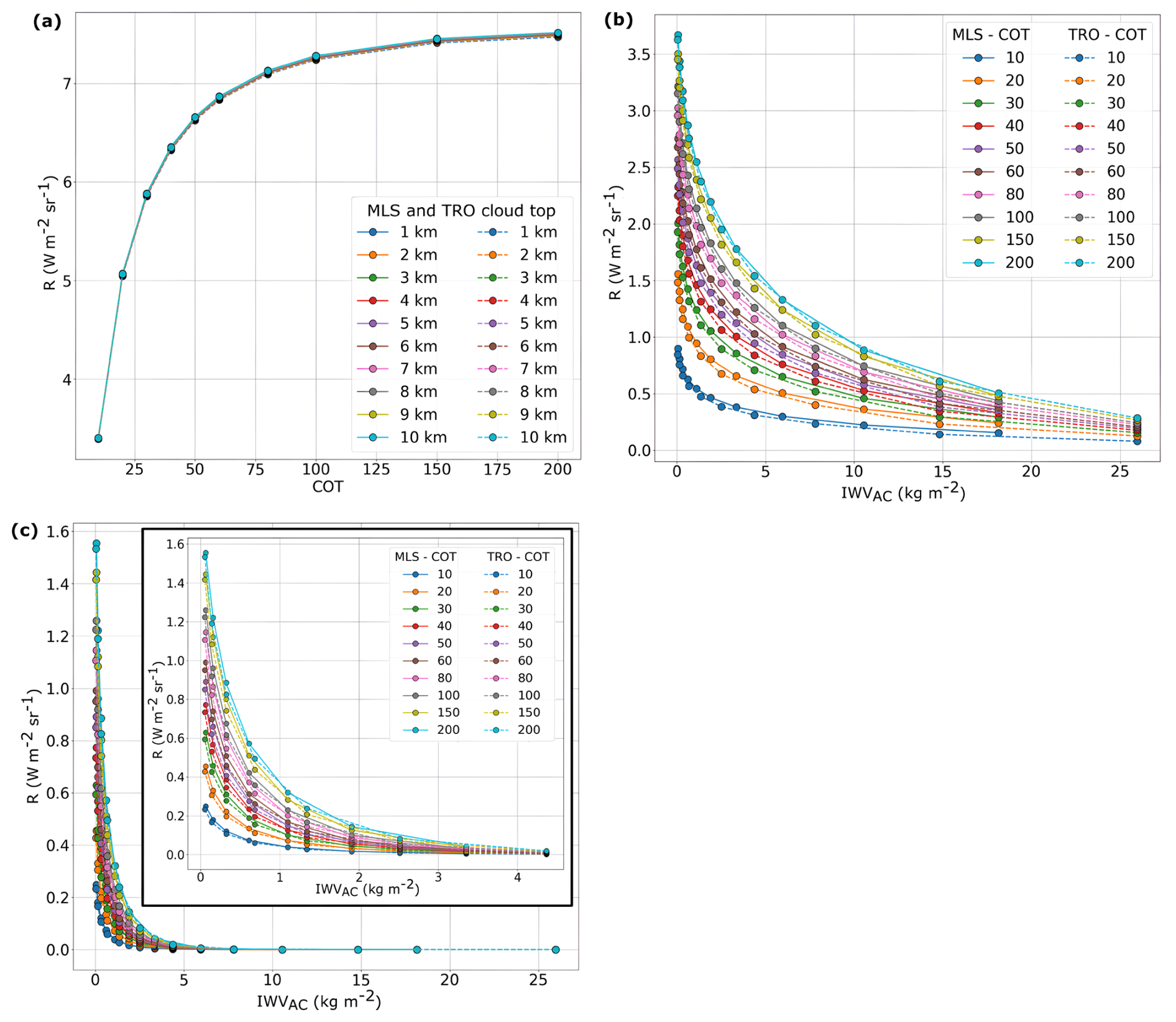
Figure 3 Simulated radiances of the C³IEL 1.04 µm band as a function of the COT (a), of the 1.13 µm band (b) and 1.37 µm band (c) as a function of IWV_AC for two atmospheric profiles from the AFGL database (Mid-Latitude Summer and Tropical profiles), for several cloud top heights (Z_t=1, 2, 3, 4, 5, 6, 7, 8, 9, and 10 km), and various COT ranging from 10 to 200. In the figure (c), the rectangle represents a zoom of the figure for IWV_AC values between 0 and 5 kg m⁻². The Solar Zenith Angle (SZA) is set to 30° and the satellite observation angle (View Zenith Angle – VZA) is 0° (nadir).

To perform this sensitivity study we introduced a set of one hundred different clouds by combining ten different cloud top heights (Z_t) ranging from 1 to 10 km in order to have a large variability of IWV_AC (from 10⁻² to 25 kg m⁻²) and ten different cloud optical thicknesses (COT) ranging from 10 to 200.

Figure 3a shows the relationship between the radiance of the non-absorbing band according to the COT for two atmospheric profiles under the 1D cloud homogeneous assumption. The relation is monotonically increasing and non-depending on the water vapor absorption as excepted from the transmission curve shown in Fig. 1. This band is thus necessary and useful to obtain information on the COT.

Figure 3b shows the results for these various cloud cases and exhibits, logically, a decrease in the simulated radiances as the IWV_AC increases with a decrease of the cloud top. Indeed, the greater the apparent radiation path through the atmosphere is, the more water vapor the radiation interacts with, leading to a decrease in radiance. Radiance sensitivity is particularly high at lower water vapor contents but decreases as the water vapor content increases.

Figure 3c shows that radiance in the 1.37 µm spectral band becomes negligible when water vapor content exceeds 5 kg m⁻². It does not reach zero in the 1.13 µm band for values until 25 kg m⁻². The 1.37 µm band is thus mainly useful in retrieving IWV_AC for low water content above cloud either in the presence of high-level clouds or in a dry atmosphere. It is also worth noting the non-overlapping color curves, where each color corresponds to a specific COT value. The differences between the curves indicate a sensitivity of the two absorbing spectral bands to the 1D equivalent COT. This value is obtained using the information contained in the non-absorbing band centered at 1.04 µm. The hypothesis of a 1D homogeneous cloud assumption with a uniform extinction vertical profile is used and leads to errors in the IWC_AC retrieval as it will be discussed in Sect. 5.2.4.

5 IWV_AC retrieval

First, the retrieval algorithm presented in this paper is tested under idealized cloudy sky profiles using clear sky profiles from the AFGL database (Anderson et al., 1986), and then under realistic cloudy sky profiles, using atmospheric profiles provided by ECMWF-IFS database (https://www.nwpsaf.eu/site/software/atmospheric-profile-data/, last access: 28 November 2025) to better evaluate its performance.

5.1 Using idealized cloudy profiles

This test set was built using the same approach as for the sensitivity test above, we artificially introduced a set of one hundred clouds in the AFGL database profiles, with a fixed cloud base height (Z_b) of 0.5 km and ten different cloud top heights ranging from 1 to 10 km. These artificial clouds are assumed to be composed entirely of water droplets with an effective radius of 10 µm and with a COT varying from 10 to 200. The solar incidence angle is set to 30° and the satellite observation angle is 0° (nadir). The target IWV_AC values are derived from the AFGL tropical profile, while the first guess profile used to start the retrieval process is the SAS (Sub-Arctic Summer) profile, due to its smooth gradient from the top to the bottom of the atmosphere. Tests carried out with different first guess profiles, both in idealized and realistic scenarios, show that initial profile has an impact on in-cloud water vapor since we assume that RH =100 % between cloud base and cloud top altitudes. So, starting iterations with the smooth SAS profile leads to an underestimation of the in-cloud water vapor absorption as the SAS profile is drier than the tropical profile used to generate the test data.

As the retrieval of COT from non absorbing wavelength is well-known, figures related to the COT retrieval are not displayed here. Nevertheless, the developed retrieval algorithm allows to retrieve 1D equivalent COT with an average error less than 12 % for COT values below 100 (less than 8 % for values below 50). However, as it is well-known (e.g., Nakajima and King, 1990; Nakajima et al., 1991), if the 1D equivalent COT exceed 100, an accurate retrieval becomes difficult because of the asymptotic behavior of the radiances for large COT values (an average error of around 43 % in this case). When COT is correctly retrieved, the in-cloud extinction profiles are identical in the simulated observations and in the model used for the retrieval. The differences in IWV_AC are thus explained mainly by the differences of in-cloud water vapor profiles. For optically thick clouds COT is systematically underestimated leading to an underestimation of the in-cloud extinction coefficient. Although radiation penetrates less in optically thick clouds, the underestimation of the COT leads to more radiation interaction with in-cloud water vapor at the top of the cloud in the retrieval algorithm than in reality.

The IWV_AC retrieval is tested for two measurement vectors: the first one with only the 1.04 and the 1.13 µm radiances and the other one with the three spectral bands centered at 1.04, 1.13 and 1.37 µm. Absolute errors (retrieved minus target values) are displayed in Fig. 4.

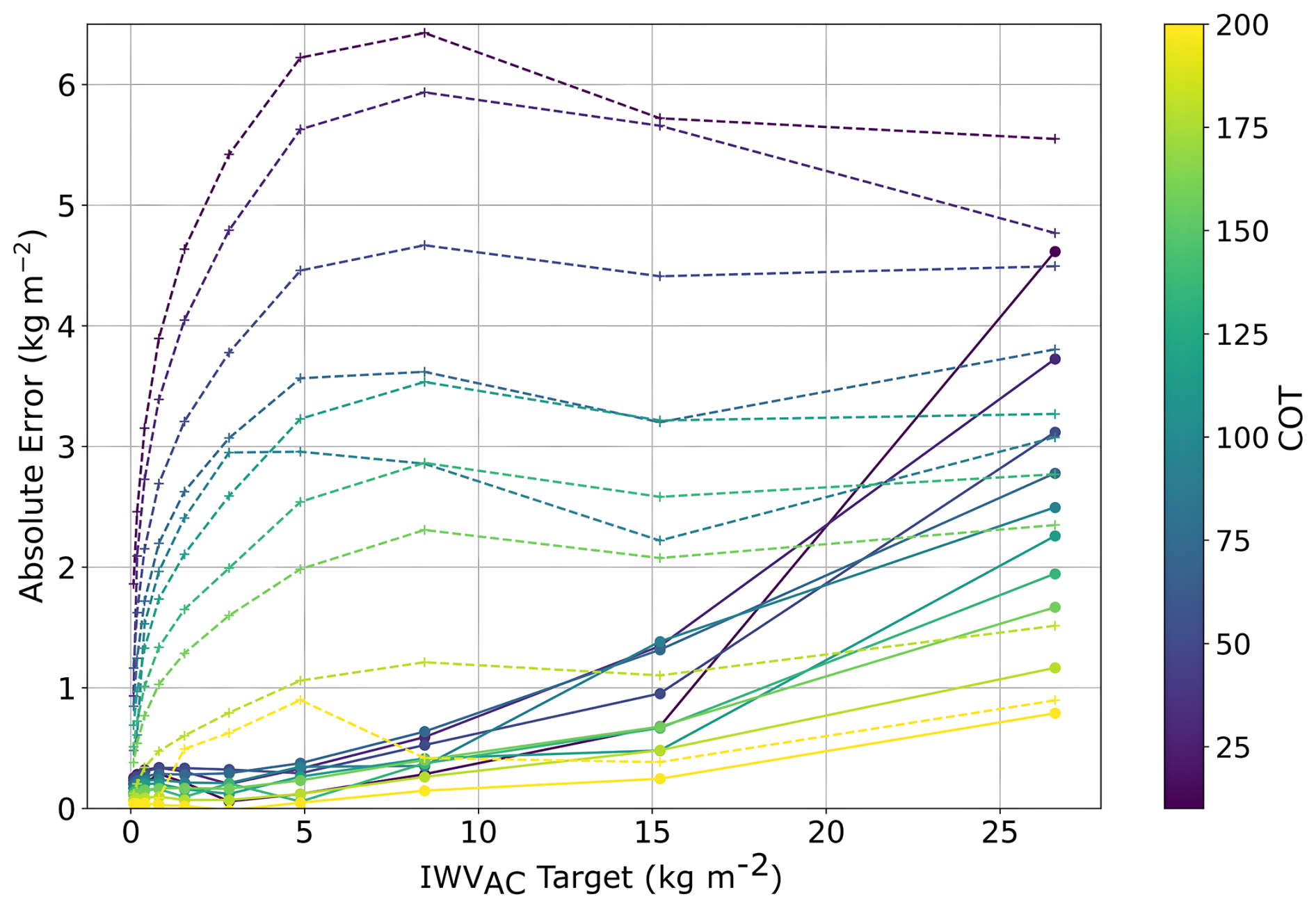
Figure 4 Absolute errors obtained for the IWV_AC retrieval (IWV_AC retrieved minus IWV_AC target) as a function of the IWV_AC target values. Dotted lines represent results obtained using only the 1.04 and 1.13 µm spectral bands, while full lines illustrate results using the three spectral bands (1.04, 1.13 and 1.37 µm) in the measurement vectors. The colorbar represents the different COT values.

While both the 2-channel and 3-channel retrieval approaches show an increase in absolute error (IWV_AC retrieved minus IWV_AC target) with increasing water vapor content and decreasing COT, the 3-channel method exhibits a more consistent, nearly monotonic error growth with water vapor. In contrast, the 2-channel method performs reasonably well up to 5 kg m⁻², but the error tends to flatten between 5–10 kg m⁻² and beyond. The absolute error is positive, indicating that the retrieved IWV_AC is overestimated due to less in-cloud water vapor absorption. This occurs because the water vapor profile within the cloud is not adjusted during the retrieval process, and the first-guess profile (AFGL SAS) is drier than the target AFGL tropical profile. Consequently, less radiation is absorbed within the cloud with the AFGL SAS model used for retrieval than with the AFGL tropical model used to simulate the test measurements. To compensate for this lower absorption and minimize the difference between the forward model simulations F(x) and the measurements y, the retrieved integrated water vapor above the cloud is overestimated. For optically thick clouds, the same behavior appears to a lesser extent, since less radiation interacts with the in-cloud water vapor.

Tests made using the tropical profile as the first guess in order to have the same in-cloud water vapor absorption between the simulated measurements and the retrievals leads to smaller errors for thin clouds since the COT is well retrieved. Conversely, larger negative errors for low-level and optically thick clouds occur, as the algorithm underestimates the in-cloud extinction profile. Consequently, there is more in-cloud absorption and the algorithm underestimates water vapor above clouds. Based on these results, the use of the SAS profile as a first guess appears to introduce a compensatory effect that partially mitigates the systematic underestimation of large COT.

When considering only the simulated radiances at 1.04 and 1.13 µm (dotted lines in Fig. 4), absolute errors increases rapidly for low IWV_AC values (below 5 kg m⁻²), to reach a peak above 6 kg m⁻² in the presence of optically thin clouds contrary to the retrieval with the three bands for which the absolute error remains less than 0.5 kg m⁻². These results clearly shows that the highly absorbing band at 1.37 µm is essential to retrieve low water vapor content above clouds. Above 5 kg m⁻² the absolute errors values with two spectral bands remain roughly constant and get closer to the errors obtained using the three spectral bands as the 1.37 µm tends to be totally absorbed (radiances are close to 0).

When examining the combined information from the three spectral bands (solid lines), the absolute errors are significantly lower than 1 kg m⁻² for water vapor contents below 10 kg m⁻², regardless of the optical thickness. As mentioned previously, as IWV_AC increases, the absolute errors also increase, particularly for thin clouds. In this case, we observe maximum absolute errors of about 3 to 5 kg m⁻² for cloud optical thickness (COT) values below 30. For optically thick clouds (COT >80), the errors remain below 2 kg m⁻², even for higher IWV_AC values. Overall, this figure highlights the necessity of using the three C³IEL spectral bands to retrieve accurately the IWV_AC, and demonstrates good performance, especially for moderate to high optical thicknesses.

Note that C³IEL will not give information about the cloud base altitude, for the idealized case we use 0.5 km and a standard deviation obtained from the ECMWF-IFS database. In order to test the sensitivity of the proposed algorithm to this fixed parameter, we performed the retrievals by adding a large error on this parameter (2000 m).

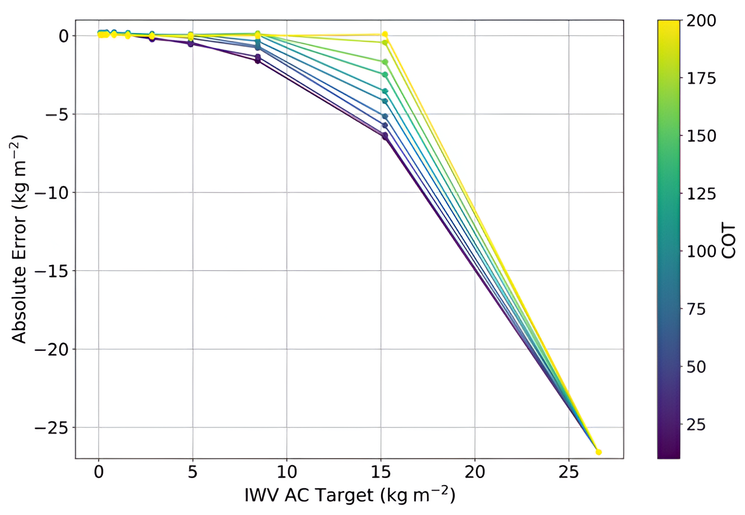
Figure 5 Same as Fig. 4 for the three spectral bands (1.04, 1.13 and 1.37 µm) configuration but with a large uncertainty of 2000 m for the cloud base altitude identified as a non-retrieved parameter.

Figure 5 shows these retrievals. Using the 3-channels approach, for cloud top altitude of 1 km, the algorithm do not converge. For low-level clouds with cloud top altitudes of 2 and 3 km, large absolute errors are observed (around −5 to −2 kg m⁻², respectively for moderate COTs, purple to blue lines). Above these altitudes, for cloud tops from 4 to 10 km, this parameter does not significantly modify the results, and absolute errors are in the same range as previously.

5.2 Using realistic cloudy profiles

The ECMWF-IFS database provides realistic atmospheric cloud profiles at 137 pressure levels, including profiles of temperature, specific humidity, cloud liquid and ice water, along with fractional cloud cover. It also provides surface data such as pressure, temperature and albedo.

5.2.1 Description of the realistic water vapor profiles

We restrict our analysis to profiles with clouds over the ocean to minimize surface effects (e.g., land, ice, snow), since the developed algorithm does not currently account for the underlying surface. Profiles at latitudes higher than 60° N/S are also excluded, since the C³IEL mission will not observe at these latitudes because the stereo-restitution algorithm for the CLOUD imager (e.g., Dandini et al., 2022) is expected not to work well with low solar incidence, and also because convective clouds in development stage, not numerous at high latitude, are the main targets of the C³IEL mission. Additionally, as the C³IEL mission focuses on studying cumulus congestus and cumulonimbus clouds, clear sky profiles and those containing only cirrus clouds have been discarded from our study, as well as we choose to study single-layer clouds, excluding cases where a clear sky layer exists between two cloud layers. The same approach was applied for selecting high-level clouds, considering only continuous clouds with the condition that the cloud top height of the liquid phase (Z_t,liq) must be greater or equal to the cloud base height of the ice phase (Z_b,ice). Figure 6 shows the geographical distribution of the 232 selected profiles of low/mid level clouds and the 30 profiles corresponding to high-level clouds. For each profile, the IWV_AC is computed and is used as the target value, considered as the “truth”. The distribution of these values are presented in Fig. 7.

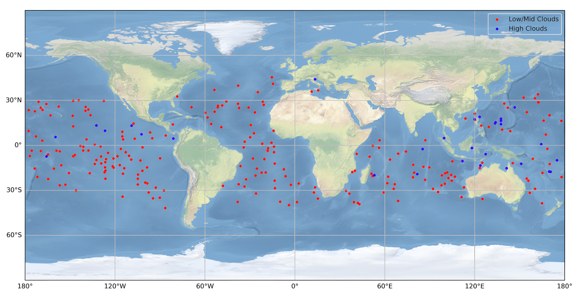
Figure 6 Geographical distribution of the selected profiles from the ECMWF-IFS database used to test the developed retrieval algorithm. A total of 262 profiles, including 232 profiles with low/mid-level clouds liquid-only clouds (red points), and 30 profiles with high-level mixed-phase clouds (blue points) are selected.

For the ECMWF-IFS profiles, the cloud base and cloud top height are obtained from the Liquid/Ice Water Content (respectively LWC and IWC) profiles. We look for the first and last values of the LWC and IWC profiles above a threshold of 10⁻³ g m⁻³. The cloud phase is determined based on the LWC and IWC values, and the layers may be classified as liquid, ice or mixed phase. Then, in case of low/mid-level clouds, IWV_AC values range from 0.5 to 21.3 kg m⁻² but are predominantly below 15 kg m⁻². Regarding high-level clouds, the values range from approximately 0.06 to 0.9 kg m⁻². Initially, the database did not include enough clouds at mid-high altitudes (6–10 km). To compensate for this deficiency, the cloud top height is artificially decreased by 4 km. As a result, the IWV_AC calculations for high-level clouds are derived from these adjusted profiles.

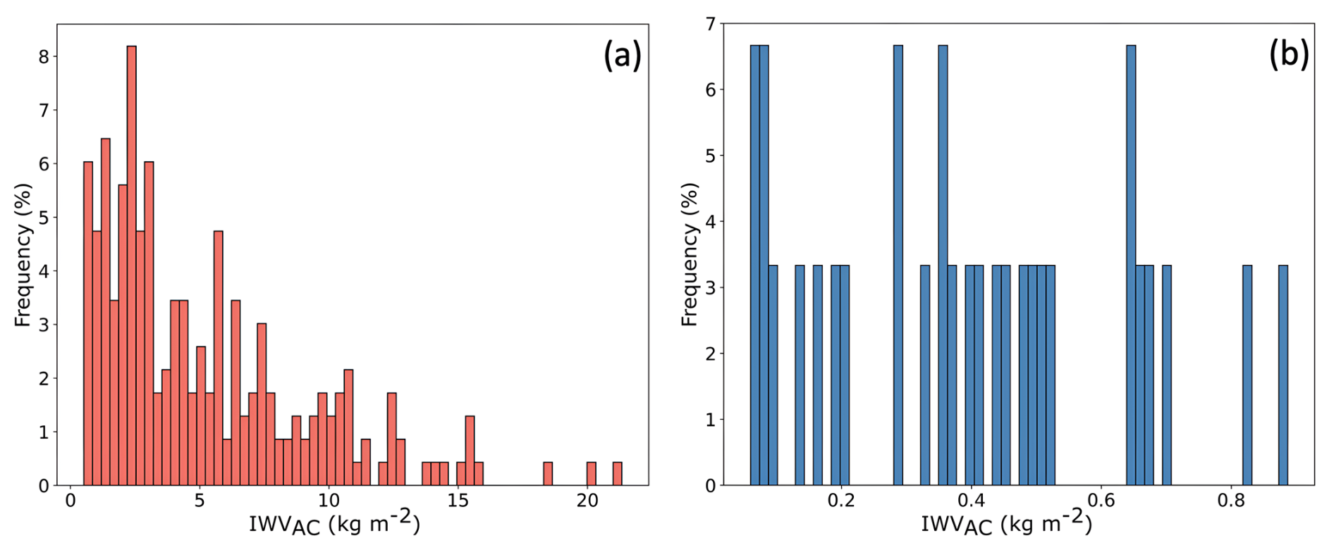
Figure 7 Distribution of IWV_AC values calculated from the selected profiles. (a) target IWV_AC values for the 232 profiles containing low/mid-level clouds, (b) target values for the 30 profiles containing high-level clouds.

5.2.2 Results of the IWV_AC retrieval: Low-/Mid-level clouds

Simulations are performed using three different Solar Zenith Angles (SZA =0, 30, and 60°) and 11 Viewing Zenith Angles (VZA), based on the C³IEL planned acquisition sequence, resulting in a total of 7656 retrievals. As for retrievals under idealized conditions, the first guess profile is the SAS profile and the figures and analyses focus only on the IWV_AC retrieval. However, the algorithm developed also allows for the retrieval of the 1D equivalent cloud optical thickness (COT) and shows an average absolute error of −2 for COT <100. In contrast, for COT >100, the COT retrieval exhibits larger errors due to the asymptotic behavior of radiance as a function of COT, as for the idealized cases. Figure 8 illustrates the relationship between the retrieved and target values of the IWV_AC along the radiation path in the atmosphere (noted mIWV_AC), where mIWV_AC is calculated as the IWV_AC multiplied by the air mass factor m, defined as:

$$\begin{array}{}\text{(7)}& m={\displaystyle \frac{\mathrm{1}}{\cos \left(\mathrm{SZA}\right)}}+{\displaystyle \frac{\mathrm{1}}{\cos \left(\mathrm{VZA}\right)}}\end{array}$$

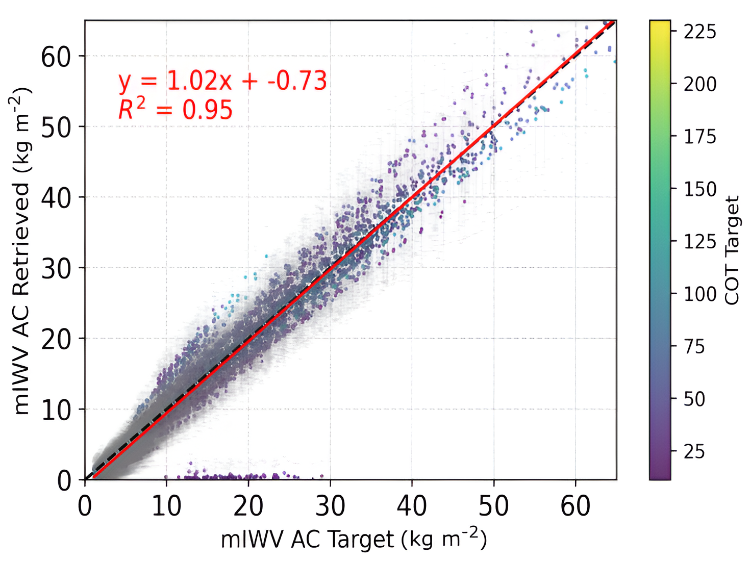
Figure 8 Relationship between the retrieved and target mIWV_AC values for profiles containing low-/mid-level clouds. The red line represents the linear regression and the black dashed line indicates the y=x line. Error bars represent the uncertainty estimated by the retrieval algorithm.

A good correlation is observed between the retrieved and target values, as indicated by a score (R²) of 0.95 and the linear regression equation as a slope of 1.02 with a small systematic under-estimation of −0.73 kg m⁻². A convergence rate of 95.8 % was achieved, indicating that 95.8 % of the profiles and geometries successfully converge to a value above the threshold limit of 0.01 kg m⁻². The 4.2 % of profiles that do not converge correspond to low and optically thin clouds, primarily clouds below 2 km and with a COT below 20, which is consistent with results obtained for idealized cases. The non convergence cases and the largest errors comes from the cloud base height (Z_b) errors and the way of computing to cloud extinction profile (C_ext), assumed to be vertically homogeneous and defined as the ratio of cloud optical thickness (COT) to its geometric thickness (Z_t-Z_b). In this study, the cloud base height is defined as the average value of the ECMWF-IFS Z_b distribution, associated with an uncertainty of 45 %, which represents, for low-level clouds, a large geometrical thickness uncertainty, impacting the cloud extinction coefficient value and the cloud vertical penetration. These results corroborate the conclusions of Albert et al. (2001) and the results obtained in Sect. 5.1.

The error bars in Fig. 8 represent the a posteriori uncertainty estimated by the retrieval algorithm. These errors comes from the errors measurement and the fixed (or non-retrieved) parameters. Although the results from the algorithm are satisfactory, only 84 % of the retrievals and their associated errors capture the target value within the 3σ confidence interval. It highlights a limitation of the current developed algorithm to perfectly take into account the errors, e.g. coming from the forward model F(x). Since no information is available regarding the “true” extinction profiles in the measurements, the typical assumption of vertical uniformity is employed, and errors related to this assumption are not included in the error variance-covariance matrix. Furthermore, after additional analysis, it was found that the unsatisfactory uncertainties correspond again to low-level clouds (Z_t<2.5 km) and/or thin clouds (COT <30). Regarding the statistics for the entire dataset, the absolute error distribution is shown in Fig. 9a. Results show an average value of −0.18 kg m⁻² and a standard deviation of 0.92 kg m⁻², indicating a small underestimation of the retrieved IWV_AC in average. To further refine and better characterize the retrieval algorithm's behavior, RMSE values have been calculated according to cloud optical thickness (COT) and cloud top height (Z_t) ranges as shown in Fig. 9b.

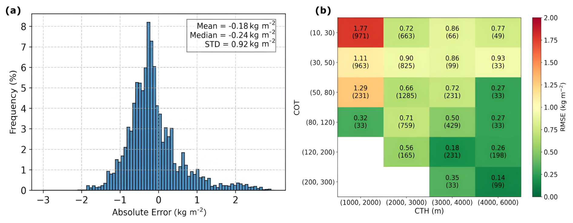
Figure 9 (a) Distribution of the absolute error (retrieved minus target) for the whole dataset, and (b) RMSEs calculated according to various Z_t, and COT ranges.

As already seen for idealized cases, the RMSE values for IWV_AC are clearly higher for low-level and thin clouds, with values generally exceeding 1 kg m⁻². The RMSE decreases as Z_t and COT increase. RMSE values are below 0.8 kg m⁻² for Z_t>2000 m and COT >50 and reach around 0.35 kg m⁻² for Z_t>3000 m and COT >120. In optically thicker clouds, the penetration of radiation into the cloud-top layers is reduced, minimizing the impact of the extinction and water vapor profile assumptions used in the forward model. Additionally, as the cloud altitude increases from low to mid-level, the IWV_AC decreases rapidly, enhancing the sensitivity of the 1.37 µm band, as demonstrated in the idealized cases (Fig. 4).

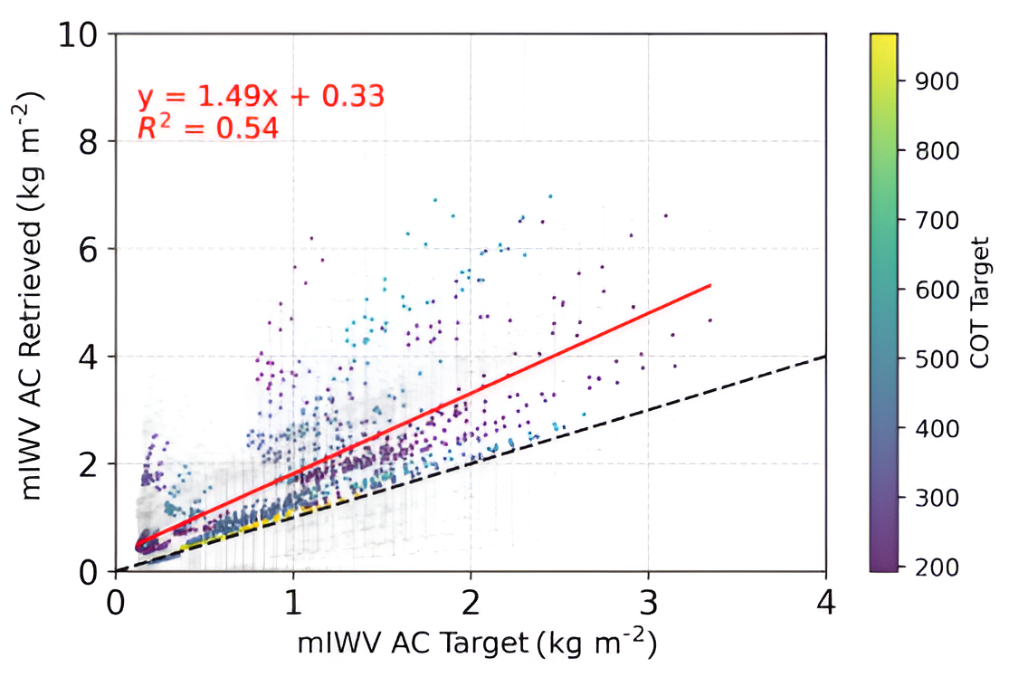
5.2.3 Results of the IWV_AC retrieval: High-level clouds

As for low-/mid-level clouds, retrievals have been calculated for the same 33 geometries, which lead to a total of 990 retrievals. Results for mIWV_AC are presented in Fig. 10. In comparison with Fig. 8, the convergence rate for high-level clouds is now 100 %. This is due to the absence of low-level or optically thin clouds in the selected profiles. For this type of clouds, COT values exceed 100 allowing the retrieval algorithm to converge for every profile. In terms of COT retrieval, the errors become considerable as beyond an optical thickness of 100, the spectral band sensitivity at 1.04 µm is not sufficient to have a reliable retrieval under the assumption of an infinite cloud. The extinction profile in the cloud model used for the retrieval is thus impacted accordingly. Regarding the mIWV_AC retrieval, the algorithm tends to overestimate the mIWV_AC retrieved value for most of the cases with a linear regression slope of 1.49 and a relatively important dispersion as the R² score is 0.54. These less favorable results, compared to the low- and mid-level cloud cases, are primarily due to six profiles (198 retrievals) where large discrepancies exist between the observed extinction profiles and those assumed in the retrieval algorithm, as discussed in the following section. Overall 76 % of the retrieved mIWV_AC values and their uncertainties capture the target values for high-levels clouds (within the 3σ confidence interval), with a global IWV_AC RMSE of 0.33 kg m⁻².

Figure 10 Same as Fig. 8 but for profiles containing high-level clouds.

5.2.4 Discussion concerning the underestimation or overestimation of the retrieved IWV_AC

As stated in the Fig. 10 comments, there is a quasi systematic overestimation of the retrieved IWV_AC value for the high-level clouds while there is a small underestimation in the case of low-/mid-level clouds (Fig. 9a).

We identified three cases that explain the underestimation, Fig. 11a, or overestimation, Fig. 11b and c, of the water vapor content above the clouds. In this figure, realistic absolute humidity (black dashed lines) and extinction profiles (green dashed line) within the cloud (obtained from the ECMWF-IFS database) are plotted alongside profiles retrieved with the forward model assumptions. The dark green lines represent vertically uniform cloud extinction profiles, while the solid red lines depict water vapor profiles, assuming 100 % relative humidity within the cloud for the SAS profile. The cloud top height (Z_t) and cloud base height (Z_b) are delimited by yellow horizontal lines.

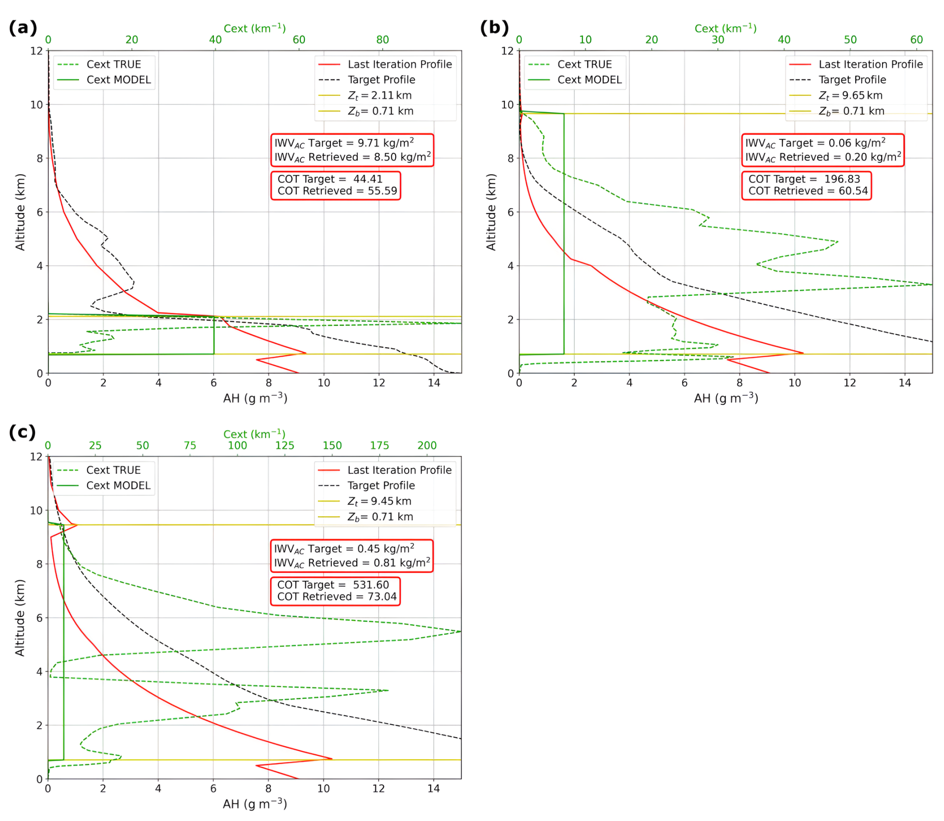
Figure 11 Absolute humidity and extinction profiles derived from the ECMWF-IFS database and retrieved from the developed retrieval algorithm. Three cases are showed to illustrate the underestimation of IWV_AC for low-/mid-level cloud cases in (a), the overestimation of IWV_AC for the high-level clouds in (b) and (c). The dashed black line indicates the “true” water vapor profile and the solid red line, the water vapor profile obtained at the last iteration of the OEM. The dashed green curve represents the “true” cloud extinction profile while the solid green line corresponds to the cloud model extinction profile. Z_b and Z_t are represented by horizontal yellow lines.

In Fig. 11a, the extinction coefficient in the upper cloud layers is lower in the model compared to the “true” extinction profile. This leads to deeper vertical penetration of radiation into the cloud compared to the realistic profile, resulting to increase the absorption by water vapor within the cloud. To compensate for this effect, the retrieval algorithm reduces absorption above the cloud resulting in lower IWV_AC (8.50 vs 9.71 kg m⁻²) in order to minimize the difference between the measured (y in Eq. 1) and simulated radiances F(x,b).

In Fig. 11b, although the algorithm tends to underestimate the total COT, it overestimates the extinction profile in the upper layers (above 7 km). This overestimation reduces the cloud penetration and, consequently, the in-cloud absorption. To compensate this effect the algorithm overestimates the IWV_AC (0.20 vs 0.06 kg m⁻²). Additionally, the in-cloud water vapor profile (dashed black line) is higher in the realistic profile. When combined with the greater radiation penetration, this amplifies the absorption difference between the target and the retrieved value, further contributing to the overestimation.

Figure 11c shows a second example that leads to an overestimation of the retrieved IWV_AC. In this case, the algorithm underestimates the retrieved COT but the extinction profile within the upper part of the cloud is very similar to the observed one, which means that cloud penetration between the observation and the retrieval is consistent. The main difference lies in the in-cloud humidity profile which is largely underestimated in the model, leading to less in-cloud absorption and thus an overestimation of the IWV_AC.

The combined effects of under/overestimation of the top layers extinction coefficient and the under/overestimation of the in-cloud humidity are certainly the main source of errors in the current algorithm. Note that these effects can sometimes counterbalance each other, for example in case of less vertical penetration into the cloud associated to higher absolute humidity values.

6 Conclusions

The objective of this study is to show the feasibility of estimating the integrated water vapor content above cloud (IWV_AC) and the cloud optical thickness (COT), in the context of a future space mission project named C³IEL (Cluster for Cloud evolution, ClImatE, and Lightning) in order to develop a retrieval algorithm, tested above ocean surfaces to minimize the effect of the surface, and it excluded high latitudes, above 60° N/S as the C³IEL instruments will not acquire measurements at these latitudes. This mission aims at investigating the development of convective clouds with a high spatial and temporal resolution, the electrical activity associated with these clouds, and the water vapor content above and around cloud. The developed algorithm is based on a Bayesian probabilistic approach, the Optimal Estimation Method (OEM), which is an iterative fitting method. It is similar to the least square method but it offers additional possibilities as it permits to consider not only the measurement itself but also supplementary information (fixed parameters, a priori knowledge, etc.) as well as associated uncertainties for the estimation of several variables.

A study has been conducted to evaluate if the three SWIR spectral bands of the C³IEL mission can be used to retrieve the integrated water vapor content above cloud (IWV_AC). First, using simulations in the two water vapor spectral bands (1.13 and 1.37 µm), we show that radiance values decreases as IWV_AC increases because of the water vapor absorption. We note that the simulated radiances in the highly absorbing band (1.37 µm) tends toward 0 for IWV_AC values greater than 5 kg m⁻², i.e., emphasizing the fact that this band is mainly useful for low IWV_AC, in dry atmosphere or above high clouds.

The developed algorithm is then first tested under idealized cloudy sky conditions with homogeneous cloud extinction profiles as assumed in the inversion model. The absolute errors of IWV_AC tends to increase as IWV_AC increases and COT decreases, thus the vertical penetration in the cloud. We also demonstrate the advantages of combining the two water vapor spectral bands, specifically, for the low water vapor content values where the absolute errors when combining the two spectral bands remains below 0.5 kg m⁻², regardless of the cloud optical thickness.

Then, the algorithm was tested on realistic profiles obtained from the ECMWF-IFS database. We focused on profiles featuring exclusively cloudy sky conditions over the ocean and within a latitude range of 60° N/S. We identified 232 cloudy profiles containing low-/mid-level clouds and 30 profiles containing high-level clouds (excluding cirrus). The algorithm exhibited a 95.8 % convergence rate for realistic profiles with low-/mid-level clouds. The IWV_AC results show a good correlation between the retrieved values and the target values (R² of 0.95 and a slope of 1.02). The RMSE is below 1 kg m⁻² for COT values above 50 and Z_t>2000 m. The RMSE tends to increase for low clouds and low cloud optical thickness. In case of high clouds, the IWV_AC values are low so more difficult to retrieve. The RMSE is however still less than 1 kg m⁻². The linear regression slope is 1.49 and the score is 0.54. The analysis shows that the errors comes mainly from the extinction profiles and water vapor profiles assumed in the inversion model.

The algorithm presented in this paper is a preliminary one and could be improved. This first version of the algorithm is currently over ocean with a constant surface albedo. In future versions, more realistic surfaces could be implemented using wind speed and the Cox and Munk (1954a, b) model above ocean, and surface albedo above continents coming from ancillary data such as ECMWF-IFS data for wind speed and MODIS or Sentinel-2 products for surface albedo values. Another way can be to use a more typical and realistic cloud extinction profiles in both liquid and mixed-phase clouds. This non-uniform profile can use a simple parametrization (e.g., Matar et al., 2023) or be based on radar measurements (e.g., Carbajal Henken et al., 2014). This improvement could possibly reduce the bias. Once the definition of the vertical profile in the algorithm has been improved, one way to test it with realistic convective cloud profiles could be to use LES simulations or the EarthCARE reconstruction (Barker et al., 2011). The cloud model phase used during the retrieval process can also be improved, particularly the assumption of 4 km made for the top of the liquid phase, for tests on high-level clouds, given that supercooled liquid clouds can be present well above 4 km altitude. Indeed, assuming that all cloud particles above 4 km are considered as ice may introduce non-negligible uncertainties. In the SWIR spectral range, this assumption is likely to lead to lower simulated reflectances, resulting in an underestimate of cloud optical thickness and biases in the retrieved microphysical parameters (e.g., King et al., 2013). Consequently, a similar effect can be expected in our case. We have shown that COT retrieval affects the IWV_AC retrieval, and since the representation of the cloud thermodynamic phase directly impacts COT retrieval, it consequently also indirectly influences the IWV_AC retrieval. A better definition of the cloud phase would therefore allow for a better representation of the cloud optical properties. To determine the cloud top phase, we plan to use the 670 nm channel from the CLOUD imager since the ratio between the visible and the SWIR non-absorbing channel (1.04 µm) provides information on the cloud top phase (Riedi et al., 2010). In case of liquid cloud, the liquid cloud algorithm would be applied and in case of cloud top ice phase, we will use climatological profiles to better constraint the transition altitudes. Another way relies on the fixed parameters accuracy of cloud base height and effective radius, which both significantly affect cloud extinction values and difference in cloud vertical penetration. To improve the determination of these values, climatological data of Z_b or R_e, specific to the geographical location of the measurements could be used. In the same way, temperature profile climatology could be used to better constrain the RH =100 % assumption in the cloud model. Furthermore, research works have to be done to exploit the multi-views of the C³IEL mission. The use of two simultaneous view angles should help reduce the uncertainties by better constraining the retrieval. However, using acquisitions spaced 20 s apart requires the development of a more complex algorithm, as the retrieved cloud top height is expected to vary sufficiently between two successive acquisitions (e.g., Dandini et al., 2022). Moreover, at the observation scale of approximately 125 m, 3D radiative transfer can introduce effects such as radiative smoothing (e.g., Marshak, 1995; Davis et al., 1997), as well as illumination and shadowing Várnai (2000) that roughen the radiative fields. These factors influence shortwave radiances and may impact the retrieval of water vapor content above clouds even if 3D radiative effects are anticipated to impact both absorbing and non-absorbing bands similarly due to their close spectral proximity. However, in addition for tilted view geometry of a finite cloud, the cloud base may appears significantly higher in the atmosphere than assumed in the cloud model, which could impact retrieval accuracy. To assess the assumption of a flat, homogeneous, and infinite cloud, more realistic cloud representations using 3D radiative simulations would be required to compute the measurements. This is a significant task beyond the scope of this paper, which aims to explore, as a first step, the possibility of retrieving integrated water vapor above clouds.

Appendix A: Variables from the a posteriori variance-covariance matrix

In our study, the a priori variance-covariance matrix (see Eq. 4) is a diagonal matrix where the diagonal terms are the squared standard deviations for each parameter contained in the a priori state vector:

$$\begin{array}{}\text{(A1)}& {\mathbf{S}}_{\mathrm{a}}=\left[\begin{array}{cc}{\mathit{\sigma }}_{\mathrm{COT}}^{\mathrm{2}}& \mathrm{0}\\ \mathrm{0}& {\mathit{\sigma }}_{{\mathrm{IWV}}_{\mathrm{AC}}}^{\mathrm{2}}\end{array}\right]\end{array}$$

with σ_COT and ${\mathit{\sigma }}_{{\mathrm{IWV}}_{\mathrm{AC}}}$ obtained by multiplying the a priori state vector x_a by the arbitrarily chosen a priori error.

S_ϵ, the error variance-covariance matrix is expressed, in our study, as follows:

$$\begin{array}{}\text{(A2)}& {\mathbf{S}}_{\mathit{ϵ}}={\mathbf{S}}_y+{\mathbf{S}}_{\mathrm{fp}}\end{array}$$

S_y is the measurement variance-covariance matrix, and S_fp describes the variance-covariance matrix linked to the fixed parameters:

$$\begin{array}{}\text{(A3)}& {\mathbf{S}}_y=\left[\begin{array}{ccc}{\mathit{\sigma }}_{y\mathrm{1}}^{\mathrm{2}}& \mathrm{0}& \mathrm{0}\\ \mathrm{0}& {\mathit{\sigma }}_{y\mathrm{2}}^{\mathrm{2}}& \mathrm{0}\\ \mathrm{0}& \mathrm{0}& {\mathit{\sigma }}_{y\mathrm{3}}^{\mathrm{2}}\end{array}\right]\end{array}$$

and,

$$\begin{array}{}\text{(A4)}& {\mathbf{S}}_{\mathrm{fp}}=K_b{\mathbf{S}}_b{K}_b^T\end{array}$$

with,

$$\begin{array}{}\text{(A5)}& K_b={\displaystyle \frac{dF\left(b\right)}{db}}{|}_x={\displaystyle \frac{F(b+db)-F\left(b\right)}{db}}{|}_x\end{array}$$

where b represent the fixed parameter (see Table 1) and db is equal to 1 % of the fixed parameter value. S_b is a diagonal matrix whose diagonal elements represent the squared standard deviation associated with the different fixed parameters of the forward model:

$$\begin{array}{}\text{(A6)}& {\mathbf{S}}_b=\left[\begin{array}{ccccc}{\mathit{\sigma }}_{\mathrm{Albedo}}^{\mathrm{2}}& \mathrm{0}& \mathrm{0}& \mathrm{0}& \mathrm{0}\\ \mathrm{0}& {\mathit{\sigma }}_{Z_{\mathrm{b}}}^{\mathrm{2}}& \mathrm{0}& \mathrm{0}& \mathrm{0}\\ \mathrm{0}& \mathrm{0}& {\mathit{\sigma }}_{Z_{\mathrm{t}}}^{\mathrm{2}}& \mathrm{0}& \mathrm{0}\\ \mathrm{0}& \mathrm{0}& \mathrm{0}& {\mathit{\sigma }}_{R_{e,\mathrm{droplet}}}^{\mathrm{2}}& \mathrm{0}\\ \mathrm{0}& \mathrm{0}& \mathrm{0}& \mathrm{0}& {\mathit{\sigma }}_{R_{e,\mathrm{ice}}}^{\mathrm{2}}\end{array}\right]\end{array}$$

The different elements of this matrix are obtained by calculating the product of the relevant fixed parameter with the uncertainty attributed to it (see Table 1).