PV power modelling using solar radiation from ground-based measurements and CAMS: Assessing the diffuse component related uncertainties leveraging the Global Solar Energy Estimator (GSEE)

Accurate PV power production modelling requires precise knowledge of the distribution of solar irradiance among its direct and diffuse components. Since this information is rarely available, this requirement can be addressed through the use of diffuse fraction models. In this study, we try to quantify the errors in PV modelling when measurements of the diffuse solar irradiance are not available. For this purpose, we use total and diffuse solar irradiance data obtained from ground-based measurements of BSRN to simulate the PV electric output using GSEE. We have chosen five sites in Europe and North Africa, with different prevailing conditions, where BSRN measurements are available. GSEE incorporates an implementation of the Boland-Ridley-Lauret (BRL) diffuse fraction model, along with a Climate Data Interface that enables simulations across different time scales. We evaluate the capability of BRL in providing accurate estimations of the diffuse fraction under diverse atmospheric conditions, with particular attention on the presence of clouds and aerosols and assess the extent to which its associated errors propagate to energy production modelling. Furthermore, we compare GSEE outputs when using CAMS radiation time-series as input instead of ground-based measurements, to quantify the impact of the CAMS radiation product uncertainties in PV modelling.

1 Introduction

Decarbonizing the power sector in a sustainable manner is pivotal in the effort to mitigate climate change (Edenhofer et al., 2011; Owusu and Asumadu-Sarkodie, 2016; IPCC, 2022) and the large-scale deployment of Solar Energy offers significant prospects toward this objective (Kakran et al., 2024). The available solar energy is a variable source, fluctuating across different timescales with a unique solar-resource profile over individual locations (McMahan et al., 2013). Therefore, accurate solar energy forecasting and resource assessment is crucial for minimizing the risk in selecting project location, designing the appropriate solar-energy conversion technology, and integrating new sources of solar based power generation into the electricity grid (Stoffel, 2013), while short-term, intra-hour forecasts are critical for power plant operations, grid-balancing, real-time unit dispatching, automatic generation control, and trading (Pedro et al., 2017).

Extending solar irradiance forecasting to derive PV power forecasts is essential in solar energy applications. PV power modelling can be achieved through the following additional steps to solar irradiance forecasting: (i) decomposing Global Horizontal Irradiance (GHI) into Diffuse Horizontal Irradiance (DHI) and Direct Normal Irradiance (DNI); (ii) calculating the plane-of-array irradiance incident on the surface of PV planes, whether static or mounted on a solar tracking system, and (iii) simulating the PV power production primarily based on the in-plane irradiance (Blanc et al., 2017).

The scarcity of concurrent measurements of both solar irradiance components, coupled with the complexity of their theoretical computation, has driven the development of numerous empirical models for estimating the diffuse fraction (ratio of the diffuse-to-global solar radiation). A seminal contribution in this area was made by Liu and Jordan (1960), who established a correlation between the diffuse fraction and the clearness or cloudiness index (ratio of the global-to-extraterrestrial radiation). These models predominantly rely on the clearness index as the principal predictor. They are generally classified into single-predictor models and multi-predictor models, with the latter incorporating additional astronomical variables for enhanced precision (Paulescu and Blaga, 2019). Typically, these models are expressed as polynomial equations, ranging from the 1st to the 4th degree, that link the diffuse fraction to the clearness index DF = f(clearness index, ∗ params) (Jacovides et al., 2006). Boland et al. (2001) proposed the use of a logistic function instead of linear or simple nonlinear functions of the clearness index. Ridley et al. (2010) developed a multiple-predictor logistic model, known as the Boland-Ridley-Lauret (BRL), which combines simplicity and reliable performance across both the Northern and Southern Hemispheres. The BRL model extends Boland's approach by adopting the hourly clearness index as the principal predictor and introducing the following additional parameters: apparent solar time, daily clearness index, solar altitude, and a measure of the persistence of global radiation level. In the implementation of the BRL included in the GSEE, the users set as input only the hourly clearness. Moreover, this implementation adopts the updated parameters proposed by Lauret et al. (2013), which derived using data from nine worldwide locations covering a variety of climates and environments across Europe, Africa, Australia and Asia. While the existing models consider all-sky conditions, in solar energy modelling it is critical to focus on cloud-free skies, where energy production is maximized. Under such conditions, aerosols become the primary parameter influencing the distribution of solar irradiance among its components. (e.g., Blaga et al., 2024). Specifically, the BRL model accounts for aerosols indirectly through the clearness index, which is indicative of the overall atmospheric attenuation of solar radiation.

In regions dominated by abundant sunshine, such as the Mediterranean and Middle East, which are favorable for solar based power generation, the attenuation of solar irradiance is strongly influenced by aerosols, and particularly desert dust aerosols. Several studies highlighted the impact of desert dust aerosol in the downwelling solar irradiance and the energy production in these regions (Fountoulakis et al., 2021; Papachristopoulou et al., 2022; Kosmopoulos et al., 2018; Kouklaki et al., 2023). The significance of considering the effect of aerosols in short-term solar irradiance forecasting and nowcasting is emphasized by Kazantzidis et al. (2017), Raptis et al. (2023) and Papachristopoulou et al. (2024).

The Global Solar Energy Estimator (GSEE; Pfenninger and Staffell, 2016) is a widely used open access model for simulating PV power output, designed for rapid calculations and ease of use. It comes with an implementation of the BRL diffuse fraction model (Ridley et al., 2010; Lauret et al., 2013).

While PV power modelling is essential for linking solar resources to energy production, the existing literature does not adequately address its reliability under diverse atmospheric conditions. To the best of our knowledge, the existing literature does not include studies that explicitly address the uncertainties in PV energy production modeling associated with the partitioning of solar radiation into its direct and diffuse components at the model input. In this study, we supply GSEE with input data from ground-based measurements as well as from the Copernicus Atmospheric Monitoring Service (CAMS), aiming to investigate differences in PV power output simulations, which arise from providing only GHI as input radiation data. At the outset, we focus on evaluating the reliability of BRL under diverse atmospheric conditions, with particular attention to the dependence of its accuracy on the presence of clouds and aerosols. To further explore this, we conduct a sensitivity analysis using radiative transfer model (RTM) simulations under cloud-free skies. Following these analyses, we assess the extent to which the associated uncertainties in the estimation of the diffuse fraction spread to the power generation over hourly intervals. This step involves simulating PV plants with varying configurations. GSEE is also effective for analyzing trends and variability in solar based power generation through its climate interface submodule (e.g., Hou et al., 2021), where the BRL model is integrated within the internal processing chain The accuracy of the climate interface in estimating the total daily PV power output is also evaluated in this study.

2 Data and Methodology

2.1 Global Solar Energy Estimator (GSEE)

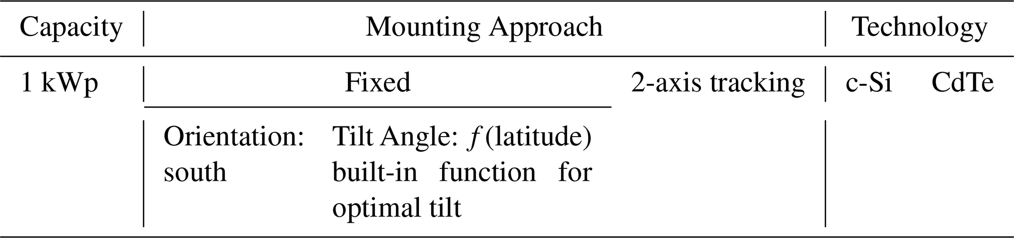
The modelling of the PV power output is conducted using the version 0.3.1 of GSEE (Pfenninger and Staffell, 2016). The model features functions for simulating a complete PV system, incorporating characteristics and specifications such as location, installed capacity, technology, tracking (fixed, 1-axis, 2-axis), tilt angle, and orientation.

The user provides as input time-series data of solar radiation, and optionally, ambient air temperature and surface albedo. Specifically, the model requires GHI and, when available, the Diffuse Fraction. If the diffuse component is not provided, the provided implementation of the BRL diffuse fraction model (Ridley et al., 2010; Lauret et al., 2013) is employed to estimate it, relying only on time-series of the hourly clearness index and the geographical coordinates. While in the single-site application of the GSEE model with hourly time resolution the user has the option to adjust the input and select alternative diffuse fraction models implemented by external libraries, e.g., pvlib (Anderson et al., 2023), the climate data interface automatically invokes the BRL model as part of the internal processing workflow. GSEE utilizes the provided information for the distribution of the irradiance components and applies trigonometric calculations to determine the total solar irradiance incident on the panel's inclined plane. More precisely, for the plane-of-array irradiance calculation a GSEE includes the submodule “trigon” (transposition model), which is based on trigonometric formulations, that account of the surface albedo, thereby including the ground-reflected component of solar radiation. However, the transposition model is integrated within the GSEE internal algorithms, so it cannot be modified by the user.

After solar irradiance the most significant parameter regarding energy production is air temperature (e.g., Dubey et al., 2013). If temperature is not provided by the user, the model assumes a default value of 20 °C. In this study, temperature was used as input only in the simulations with BSRN data, as it is provided alongside radiation measurements. A surface albedo value of 0.3 considered by default from the model, introduces some uncertainty in our simulations, which however is estimated to be small. Under cloudless conditions, a 10 % difference in surface albedo changes the GHI by ∼1 % for SZA < 75°. Differences are larger under cloudy conditions (∼10 % difference in GHI for a 10 % difference in surface albedo). Nevertheless, surface albedo at the selected sites is generally low and relatively invariant throughout the year (even at the most northern site of Lindenberg there is only a limited number of days with increased surface albedo due to snow cover).

The available options for the panel type are crystalline silicon (c-Si) and Cadmium Telluride (CdTe), where the power output is modeled based on the relative PV performance model described by Huld et al. (2010). For fixed panels, a built-in latitude dependent function for the optimal tilt is also included.

Moreover, GSEE includes a Climate Data Interface submodule that enables the processing of gridded climate datasets, with varying temporal resolutions, ranging from hourly to annual. Within the context of this submodule, the use of BRL serves as part of the resampling and upsampling processes applied to input climate datasets with daily resolution. For processing data with lower-than-daily resolutions, it incorporates the use of Probability Density Functions (PDFs), which describe the probability with which a day with a certain amount of radiation occurs within a month (GSEE, 2026). This methodology accounts for the non-linear distribution of mean monthly radiation across individual days, ensuring a more representative temporal disaggregation. The processes applied to the mean daily irradiance are described in detail in Sect. 3.4.

For the purposes of this study, we simulated solar plants with capacity of 1 kWp, and for both available technologies. The simulations with c-Si technology, considered as default by the model, are presented in detail the following sections. The results of the simulations with CdTe technology are provided in the supplement, and are not thoroughly discussed, since they are very similar to the results for the c-Si technology. Regarding the mounting approach, the solar plants were either static and oriented to the south or equipped with a 2-axis solar tracking system. In the case of fixed panels, we selected the optimal tilt angle relying on the latitude dependent built-in function.

The input parameters defining the characteristics of the simulated PV plants are summarized in Table 1.

Table 1 Input parameters defining the characteristics of the simulated PV plants.

2.2 Ground-based measurements

We supplied GSEE with ground-based irradiance as well as ambient temperature measurements collected from five stations of the Baseline Surface Radiation Network (BSRN; Driemel et al., 2018). Moreover, information about aerosols was retrieved from co-located stations of the Aerosol Robotic Network (AERONET; Holben et al., 1998; Dubovik et al., 2000).

Information for the stations utilized for this study is summarized in Table 2, and their geographical location is depicted in Fig. 1.

Table 2 Detailed information about the location of the ground-based stations used in this study.

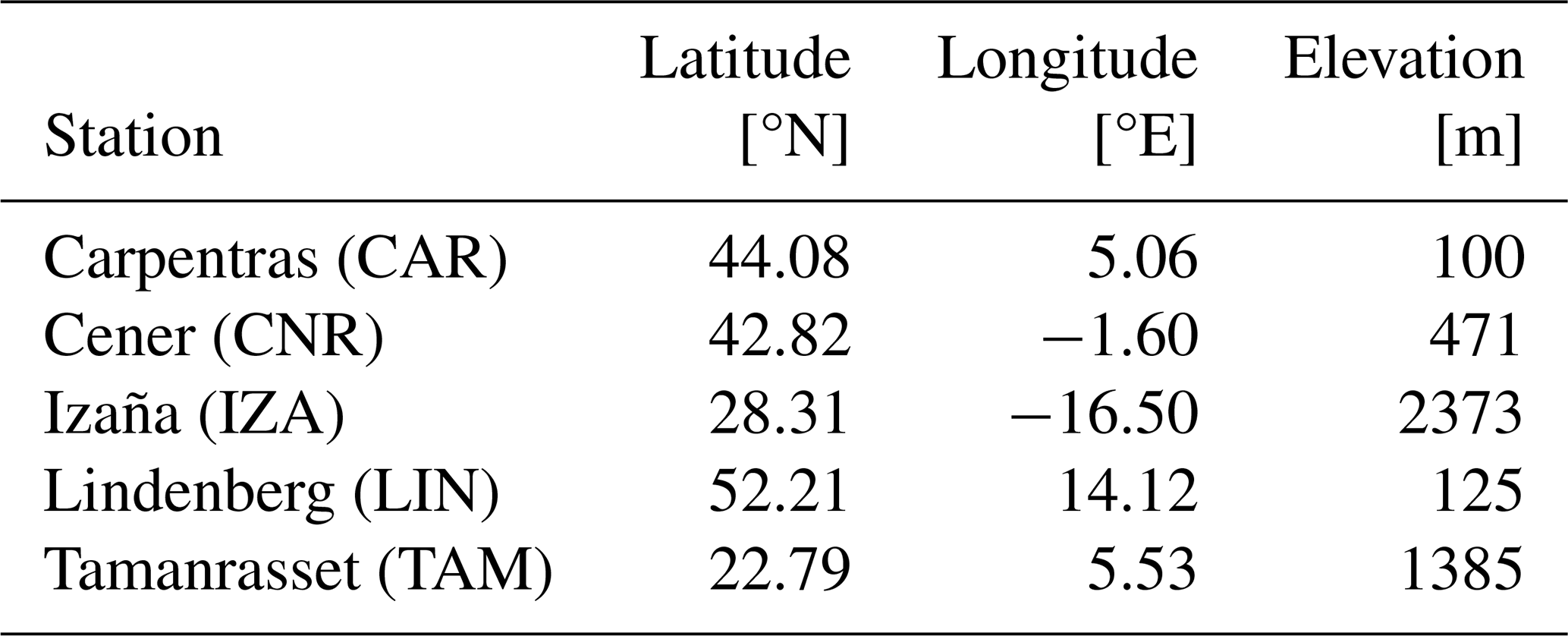
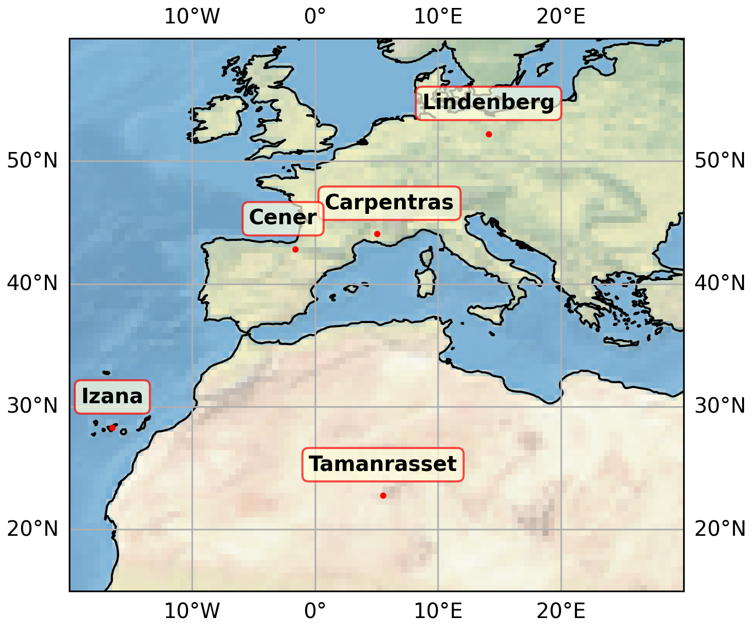
Figure 1 Locations of the BSRN and co-located AERONET stations that are used in the current study.

BSRN station-to-archive files were accessed and manipulated using the SolarData v1.1 R package (Yang, 2019), and the BSRN-recommended quality check (QC) tests (Long and Dutton, 2010) applied to the collected data. Some data gaps arose due to measurements removed during the QC procedure. Although these data gaps are, in most cases, shorter than 2–3 h, they may affect the BRL performance throughout the corresponding days. Consequently, days affected by such data gaps excluded from the analysis. We retrieved data for 2017, with 1-min temporal resolution. We used GHI, DHI, and Temperature as inputs to the GSEE model. Initially, the data were resampled to hourly and mean hourly values of GHI and DHI are calculated. Then, the simulations were conducted using either GHI and DHI, or only GHI along with the deployment of BRL. The input to BRL consists of hourly clearness index, derived by dividing GHI measurements with the solar radiation incident on a horizontal plane at the Top of the Atmosphere (TOA) above the examined location. Subsequently, the 1-min timeseries resampled also to a daily resolution and transformed into three-dimensional arrays, $\mathrm{GHI}=f\left(\mathrm{time},\mathrm{lat},\mathrm{lon}\right)$, where the spatial dimensions of each dataset corresponded to a unique point defined by the coordinates of the associated station. Simulations with the daily time-resolved dataset were performed using the Climate Data Interface.

Representing cloudiness is a challenging task that requires several observations. For this purpose, aiming to obtain an indicative measure of the intra-hour cloudiness conditions we adopted the following formulation. Specifically, measurements of Direct Normal Irradiance (DNI) were utilized to obtain information for cloudiness relying on the conditions stated by WMO (2021), according to which sunshine duration is the total period where DNI exceeds 120 W m². Alternative approaches such as the Cloud Modification Factor, require estimates of the clear sky irradiance, which introduces additional uncertainty. For the purpose of this analysis, we introduced a solar visibility (SV) parameter. Specifically, we assigned the value 0 when sun was obscured and the value 1 when visible. Aiming to describe the mean intra-hour cloudiness conditions, we considered the sky as cloud-free, cloudy, and partly cloudy based on the mean SV for the entire corresponding hour as follows:

$$\langle \mathrm{SV}{\rangle }_{\mathrm{hour}}:\left\{\begin{array}{ll}\mathrm{1}& \mathrm{cloud}-\mathrm{free}\\ \in (\mathrm{0},\mathrm{1})& \mathrm{partly}\mathrm{cloudy}\\ \mathrm{0}& \mathrm{cloudy}\end{array}\right.$$

For aerosol information, we accessed the AERONET Version 3 (V3) (Giles et al., 2019) and retrieved level 2.0 data (from direct sun measurements) for Aerosol Optical Depth at 500 nm (AOD₅₀₀), which serves as a representative measure of the aerosol load; Ångström Exponent between 440 and 870 nm wavelengths (AE_440−870), where values near 0 correspond to coarse dust particles and values around 2 to fine (e.g., smoke) particles (Dubovik et al., 2002);  and Fine Mode Fraction at 500 nm (FMF₅₀₀) obtained from the Spectral Deconvolution Algorithm (SDA) retrievals, to distinguish aerosol into fine and coarse mode. The data were resampled at hourly intervals and a mean hourly value calculated. After, the hourly mean values divided into clusters based on AOD₅₀₀, reflecting different levels of aerosol load and allowing us to quantify their impact on solar energy production. To investigate the impact related exclusively to aerosols, we included only hours with cloud-free sky conditions. The clusters are defined in detail as follows:

• AOD₅₀₀≤0.05: Low aerosol load

• $\mathrm{0.05}<{\mathrm{AOD}}_{\mathrm{500}}\le \mathrm{0.15}$: Moderate aerosol load

• $\mathrm{0.15}<{\mathrm{AOD}}_{\mathrm{500}}\le \mathrm{0.3}$: High aerosol load

• AOD₅₀₀>0.3: Very high aerosol load

To evaluate the performance of the Climate Interface over daily intervals, we defined the sunny (cloudless) days using the condition: 〈SV〉_day≥0.9. Next, to characterize the average aerosol conditions on sunny days, we applied the following classification:

• 〈AOD〉_day≤0.05: very-low aerosol

• 〈AOD〉_day>0.05: aerosol-laden

Detailed comparisons of the energy production over hourly and daily integrals under the various predefined sky conditions are provided in the supplement through evaluation metrics.

The selected locations have quite different atmospheric conditions regarding cloudiness and aerosols. Additionally, they vary in altitude. A brief overview of the prevailing conditions derived from the ground-based data is provided on the supplement. Regarding cloudiness, it is notable that in Lindenberg the sky is generally overcast, whereas in southern locations sunshine dominates. In terms of aerosols, very high aerosol loads occur more frequently in Tamanrasset. As for aerosol type, there is considerable variation among the examined locations: Carpentras, Cener, and Lindenberg are primarily influenced by fine mode aerosols, while Tamanrasset and Izaña are mostly affected by coarse mode aerosols.

For investigating the impact of desert dust aerosol in solar based power generation, Tamanrasset serves as a representative and exceptional case because it is in a region with important sources of Saharan dust aerosols (Faid et al., 2012). Meanwhile, Izaña, located in subtropical North Atlantic, is a high mountain station within the free troposphere, affected mineral dust when the Saharan Air Layer top exceeds the station height, especially through August to October (Toledano et al., 2018; Cuevas et al., 2019). Due to its high altitude, Izaña avoids contamination from local or regional sources (Barreto et al. 2022). The Canary Islands, where Izaña is located, are influenced by extreme dust events that cause a significant decrease in PV power generation (Canadillas-Ramallo et al., 2022). In South Europe, which is also affected by the transport of Saharan dust across the Mediterranean, aerosol types exhibit a mixture as a result of simultaneous local pollution and low concentration of mineral dust (Logothetis et al., 2020).

2.3 Copernicus Atmospheric Monitoring Service (CAMS)

We retrieved data from the CAMS radiation service (Schroedter-Homscheidt et al., 2022; Qu et al., 2017), from the solar radiation time-series product (CAMS, 2020). The CAMS solar radiation service provides historical estimates for global solar radiation, along with its components, from 2004 to present. These values are provided with a frequency as fine as 1-min. In this study, we used the hourly time-series of GHI and DHI for all-sky conditions, setting the input coordinates to match the locations of the BSRN stations. The solar radiation time-series product (CAMS, 2020) performs interpolations integrated in its internal algorithm and provides time-series for the coordinates and the altitude of a single-site location. We compared the solar energy production derived from the use of CAMS data with that derived from the use of ground-based measurements from BSRN.

2.4 Radiative Transfer Model (RTM)

We performed Radiative Transfer (RT) simulations aiming to further assess the uncertainties in estimating the diffuse fraction arising from the effect of aerosols. The simulations were conducted using libRadtran (Emde et al., 2016; Mayer and Kylling, 2005), a widely used software package, allowing the computation of radiances, irradiances, and actinic fluxes. A sensitivity analysis was performed by comparing the diffuse irradiance calculated from libRadtran with the estimations of BRL. This analysis examines the dependence of the aerosol-related discrepancy as function of Solar Zenith Angle (SZA) and latitude, considering the effect of parameters such as surface albedo and altitude.

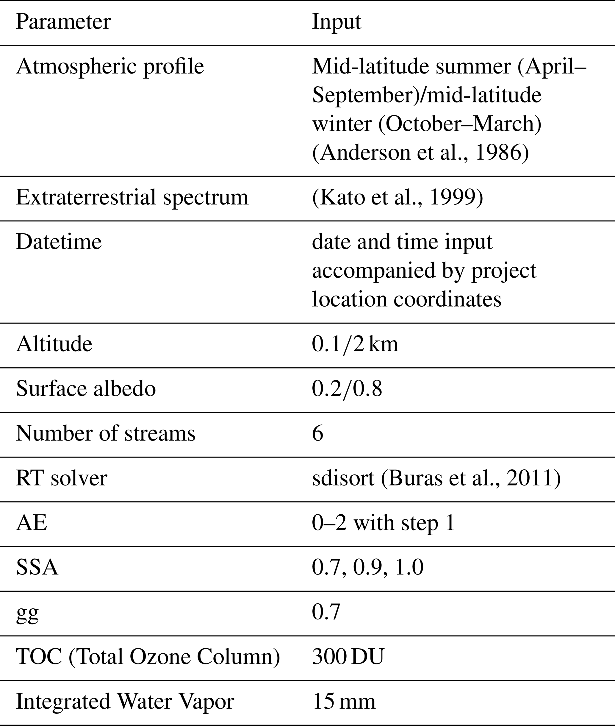
To conduct aerosol parameterizations, we considered the default aerosol extinction profile (Shettle, 1989) and set asymmetry factor (gg) to 0.7, while varying the Single Scattering Albedo (SSA) and the Ångström Exponent (AE), and defining AOD₅₀₀ by adjusting the value of the parameter-b in Ångström's law (Ångström, 1929) as follows:

$$\begin{array}{}\text{(1)}& {\mathit{\tau }}_{\mathit{\lambda }}=b\cdot {\mathit{\lambda }}^{-a}\to {\mathrm{AOD}}_{\mathrm{500}}=b\cdot {\left(\mathrm{0.5}\mathrm{\mu }\mathrm{m}\right)}^{-\mathrm{AE}}\end{array}$$

The standard aerosol profiles (Anderson et al., 1986) were used for all sites. According to Fountoulakis et al. (2022), using a more accurate vertical distribution of aerosols in the troposphere would have a negligible effect in the GHI and DHI at the Earth's surface. Table 3 illustrates the libRadtran settings used in this study.

Table 3 LibRadtran inputs.

3 Results

3.1 Performance verification of the BRL diffuse fraction model

The performance of BRL was evaluated by comparing the actual diffuse fraction, obtained directly from resampled to hourly BSRN ground-based measurements, with that derived using BRL. As a first step, to isolate the influence of SZA from that associated with the atmospheric conditions, the difference in diffuse fraction (DF) between the observed and the one estimated using BRL as a function of SZA is presented in Fig. 2. The atmospheric conditions are represented separately for both all-sky and cloud-free sky conditions and are grouped into clusters, as outlined in Sect. 2.2. The patterns reflecting the differences under the distinct sky conditions indicate an additional dependency on SZA, which becomes apparent approximately at SZA between 60 and 70°. In most cases, there is an almost constant displacement with respect to y=0 below 60°, as well as a change in behavior when SZA exceeds this value. Izaña presents a special case, as the station is located at a very high altitude. At such high altitudes the contribution of the diffuse component to the total irradiance is significantly smaller relative to lower altitude sites, which seems to be captured more accurately by BRL at high SZAs. We must also note that (i) at Izaña, the actual diffuse irradiance may experience an additional enhancement due to the contribution of adjacent lower-lying clouds – an effect that is not accounted for in the diffuse fraction model, and (ii) during dust events the site is usually inside – and not under – the dust layer, which results in more complex interactions between dust and solar radiation relative to lower altitude sites. Defining an exact limit (for the lower altitude sites), where the behavior is changing, is challenging; therefore, 60° was selected for practical energy-related applications, focusing on periods with meaningful energy contribution, and is supported by the sensitivity analysis (Sect. 3.2) under clear-sky conditions. Concerning the same grouped atmospheric conditions, Fig. 3 illustrates the comparison between the observed and the estimated diffuse fraction for SZA≤60°. This approach allows us to examine BRL performance after eliminating the influence of SZA, thereby providing a more comprehensive view of its reliability.

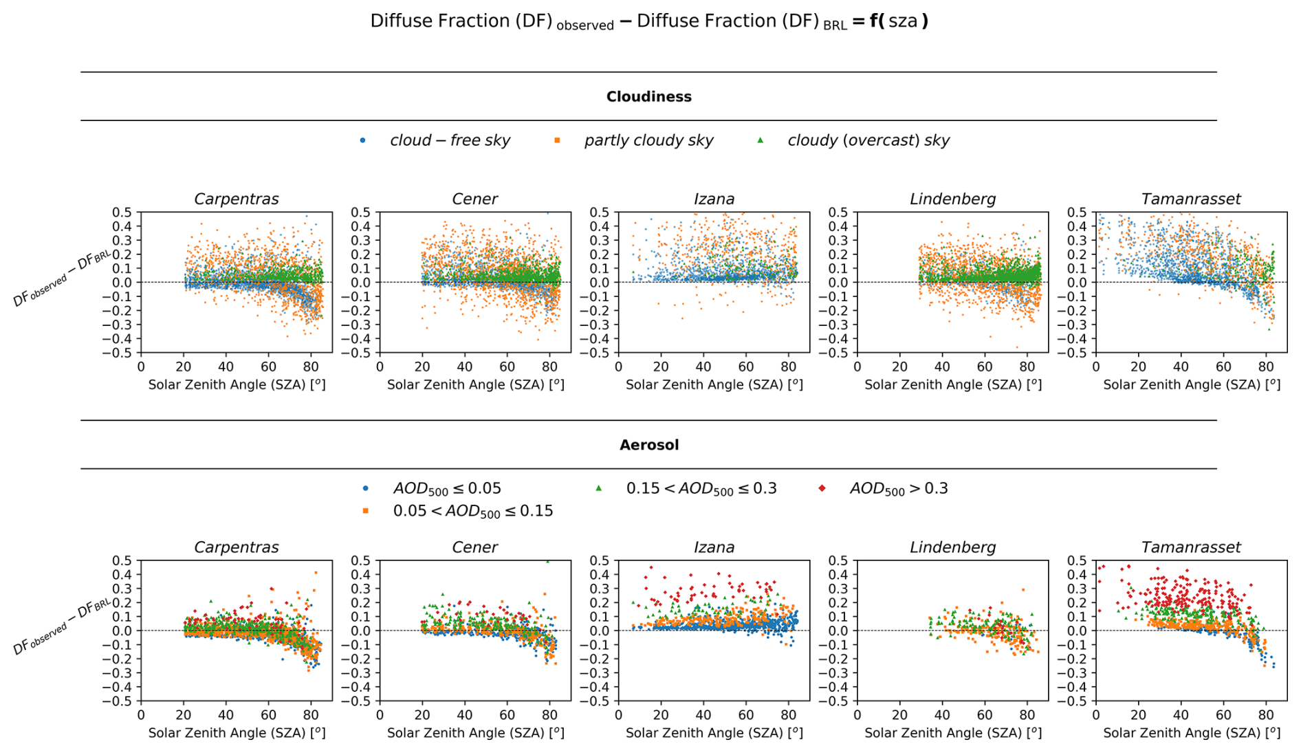
Figure 2 Difference between the diffuse fraction estimated by the ground-based measurements and by using the BRL model as a function of SZA under diverse atmospheric conditions: (top) classification with respect to cloudiness and (bottom) classification with respect to aerosol optical depth.

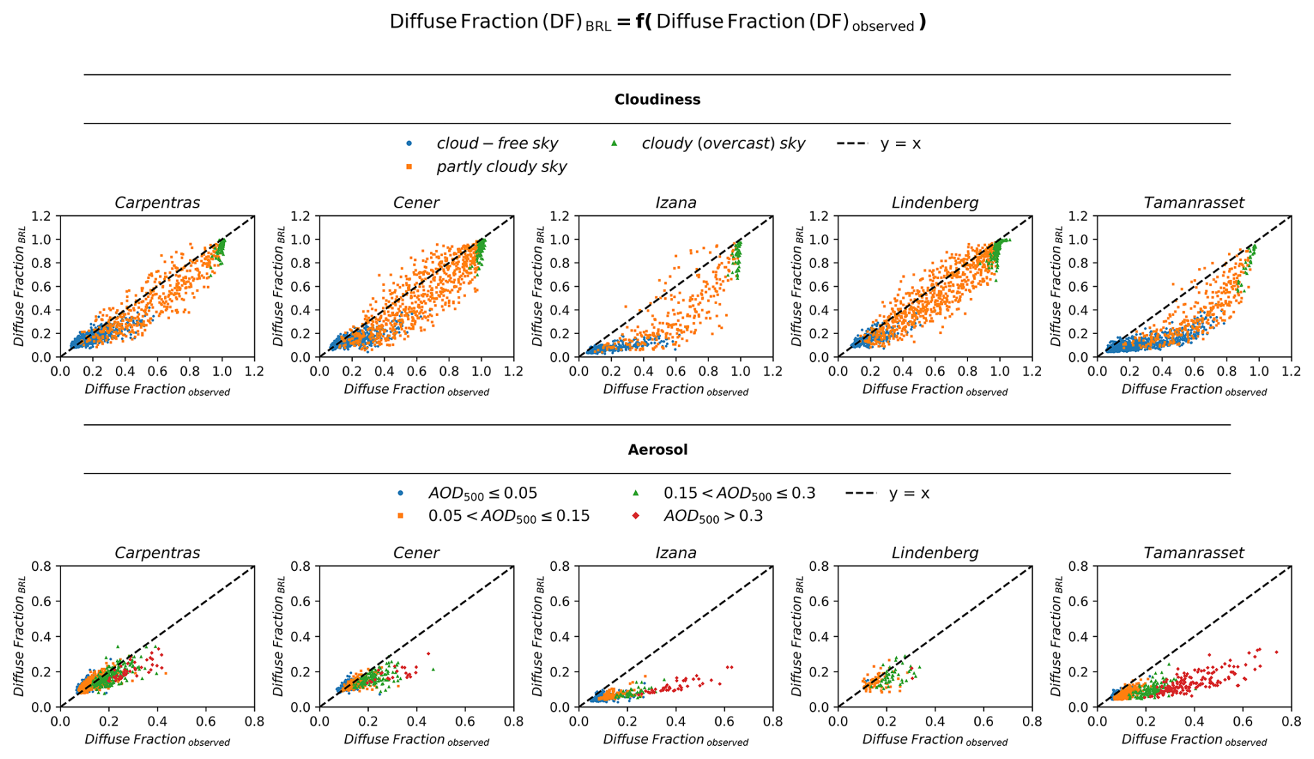
Figure 3 Comparison of the diffuse fraction estimated using BRL with that estimated by the ground-based measurements under diverse atmospheric conditions for SZA < 60°: (top) classification with respect to cloudiness and (bottom) classification with respect to aerosol optical depth.

From Fig. 3, a distinct dependency of BRL's reliability on the atmospheric conditions can be observed. Under all-sky conditions, the presence of clouds has a notable impact on the model's performance. Partly cloudy conditions result in greater dispersion of the values from the identity line respectively, likely due to the complexity of such sky scenes. Under overcast conditions, where the sky can be considered homogeneous and isotropic, the model in most cases performs slightly better. However, the limitations of the DNI-based classification methodology, related to the complexity of the cloud scenes, the spatiotemporal variability during the hourly periods, and the 3D variability of cloud properties, would require additional observational tools for a more detailed investigation. More specifically, the vast majority of overcast cases where the BRL diffuse fraction is below 0.8 while the observed is close to 1 correspond to periods involving rapid transitions between partly cloudy and overcast skies, occurring either during the hour itself or immediately before or after it. Furthermore, a limited number of cases identified during intense dust events at Tamanrasset and Izana, where the reduction of DNI was so pronounced that the applied DNI-based criterion classified these conditions as overcast. However, these cases are not further investigated, as the energy production levels during such periods are very low.

Under cloud-free skies, BRL tends to underestimate, and this bias becomes more pronounced as aerosol load increases. Aiming to highlight this dependency, Fig. 4 shows the difference between the estimated and the observed diffuse fraction as function of AOD₅₀₀, emphasizing also the extent to which it is related to the aerosol type by providing FMF₅₀₀. A decrease for increasing AOD₅₀₀ is evident across all cases. In Tamanrasset and Izaña, associated with the influence of Saharan dust, the coarse mode dominates, and a more distinct and well-defined curve is depicted compared to other sites.

It is important to clarify that for assessing the impact of aerosols we have assumed entirely cloud-free conditions. However, the criterion applied based on DNI does not fully guarantee the absence of small, scattered clouds within the sky dome. Such clouds could induce slight enhancements in DHI. A more rigorous assessment of the impact associated exclusively with aerosols could be achieved by integrating images from ground-based co-located all-sky cameras. On the other hand, the presence of aerosols even under cloudy scenes, introduces an additional uncertainty which is difficult to investigate accurately.

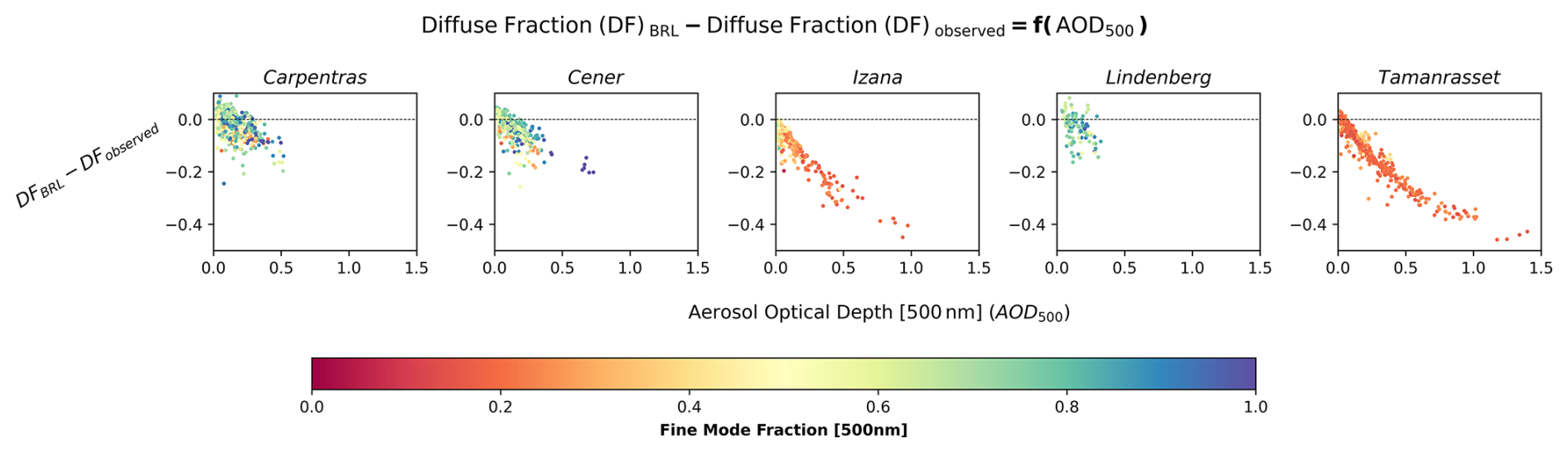
Figure 4 Difference between the estimated using BRL and the diffuse fraction estimated by the ground-based measurements as function of AOD₅₀₀ and FMF₅₀₀.

3.2 Sensitivity analysis of the BRL performance under cloud-free sky conditions from RT simulations

The uncertainties in estimating diffuse fraction under cloud-free sky conditions, as discussed in Sect. 3.1, are further investigated. We performed RT simulations using libRadtran to calculate GHI and DHI under various aerosol scenarios. The resulting GHI values were then used as input to BRL to estimate the diffuse fraction, which was subsequently compared to the diffuse fraction derived directly from the ratio of DHI to GHI computed by libRadtran.

To ensure a comprehensive analysis, we considered three representative latitudes (25, 35 and 45°). Since BRL requires an hourly time-series of GHI as input, the analysis was conducted for the summer solstice. On this day, a sufficient number of hourly values are available, corresponding to a wide range of SZA values, allowing for a robust assessment of the methodology. The sensitivity analysis was performed for surface albedo values of 0.2 and 0.8 as well as for altitudes of 0.1 and 2 km. For aerosol parameterization, we examined completely clear-sky conditions as a reference, alongside scenarios with AOD₅₀₀ values of 0.2, 0.6, and 1, while varying the SSA and AE. Specifically, the scenarios included SSA values of 0.7, 0.9 and 1, combined with AE values of 0, 1 and 2. The results of this sensitivity analysis for an albedo of 0.2 are provided in Fig. 5, while the results for an albedo of 0.8 are included in the supplement (Fig. S1 in the Supplement).

The results confirm that BRL performs well under clear sky conditions and for SZA below 60°, while the incorporation of aerosols in the sky scene introduces larger uncertainties. In all scenarios, we observe that lower values of AE correspond to higher uncertainties. Moreover, when SSA is 0.9 or 1 BRL gradually tends to underestimate the diffuse fraction as aerosol load increases. Instead, when SSA is 0.7, BRL exhibits a different behavior, shifting toward an overestimation of the diffuse fraction at high aerosol loads.

The findings of this sensitivity analysis are consistent with the evaluated BRL performance from ground-based measurements presented in Sect. 3.1, especially at SZA smaller than 60–70°, and underscore the role of aerosol in the accuracy of diffuse fraction estimations. Differences between the results shown in Figs. 2 and 5 at SZA between 60–80° can be due to a number of site-related reasons. For example, enhancement of the diffuse component due to scattering by underlying atmospheric layers and clouds in the case of Izaña may compensate the observed overestimation of the diffuse fraction by BRL. Concerning the impact related to AE and SSA, we confirm that the higher underestimations observed for Tamanrasset and Izaña are associated with the optical properties of desert dust aerosol particles. While AE and SSA alone are not sufficient to fully characterize the aerosol type, they serve as strong indicators, aligning with the classification framework of Dubovik et al. (2002). The same comparison for albedo 0.8 (Fig. S1) reveals a significant broadening of the discrepancies. Moreover, we observe the presence of a systematic error, even under clear sky conditions.

The resulting differences were practically identical across the three selected latitudes, indicating that the BRL model is largely independent of latitude and can therefore be considered as a reliable solution over a wide range of latitudes. Furthermore, the effect of altitude was found to be small. Finally, the outcomes of this analysis highlight potential inconsistencies arising from aerosols with different optical properties. Although the updated parameters of the BRL's model (as implemented in the GSEE model) reported by Lauret et al. (2013) were derived using data from nine worldwide locations, encompassing a broad range of sky conditions that capture a fully representative set of optical properties remain challenging.

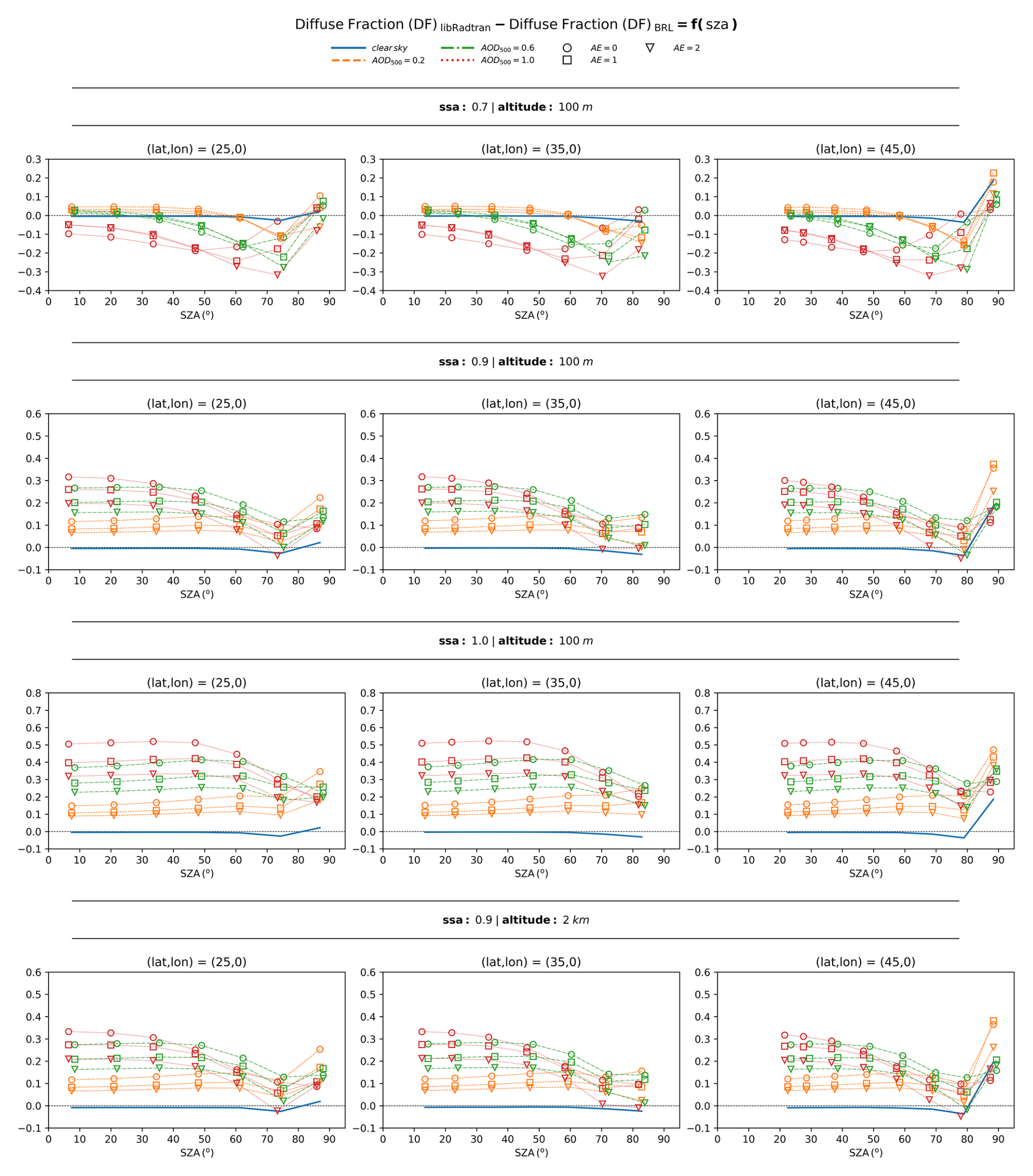
Figure 5 Difference between the diffuse fraction derived directly from the computations of DHI and GHI using libRadtran and the one estimated by applying BRL to the libRadtran-computed GHI.

3.3 Analysis of the differences in energy production using hourly integrals within the modelling of PV plants

Uncertainties in estimating the diffuse fraction influence the calculation of the total irradiance received by an inclined panel's surface, thereby affecting the accuracy of the PV power simulations. In this section, we employ the main submodule of GSEE, used for modelling the electric output from a PV panel, aiming to assess the extent to which these uncertainties propagate to the estimation of the hourly power production. We analyze discrepancies arising from using only GHI from BSRN as input radiation data to the model, instead of both DHI and GHI. More specifically, we compare the total energy produced per hour per unit, expressed in watt-hours (Wh), per unit of nominal power (kWp). The energy production is evaluated for both fixed panels and 2-axis tracking systems.

The results of this comparison for c-Si based technology PV panels for different atmospheric conditions are presented in Fig. 6, illustrating the impact of cloudiness, and in Fig. 7, demonstrating the effect of aerosols. The corresponding results for CdTe technology are provided in the supplement (Figs. S2 and S3 respectively). In the modelling of 2-axis solar tracking systems, where the panel is continuously adjusted to maintain a perpendicular orientation to incoming solar radiation, the system becomes more sensitive to uncertainties in the estimation of the diffuse fraction, leading to more significant differences in energy production. Specifically, the contribution of the direct irradiance is maximized in such systems, as the panel exploits the entirety of the available direct irradiance. On the other hand, in the simulation of static panels, the contributions of direct and diffuse components are more evenly distributed, making the impact of diffuse fraction uncertainties less pronounced in energy production.

Regarding the uncertainties related to the atmospheric conditions, from Fig. 6 we confirm that the highest dispersion occurs in partly cloudy conditions, while from Fig. 7, where we examine cloud-free conditions, we note that further improvement achieved as aerosol load decreases. Under totally overcast skies the energy production is extremely low, rendering errors practically negligible. Moreover, accuracy is influenced by aerosols, where a gradual decline in accuracy is detected as aerosol load increases. However, assessing the extent of aerosol loading impact is complex, depending on the interaction of solar radiation with particles of varying optical properties, as extensively analyzed in the previous sections. This effect becomes particularly evident in cases of high aerosol loading, where a noticeable offset is observed, while under certain conditions, the associated uncertainty is comparable to that found in partly cloudy conditions.

Figure 6 Comparison of the estimated hourly PV power generation between simulations performed using GSEE with input data consisting of either only GHI or both GHI and DHI under varying cloudiness conditions: (top) fixed panels (bottom) 2-axis tracking systems.

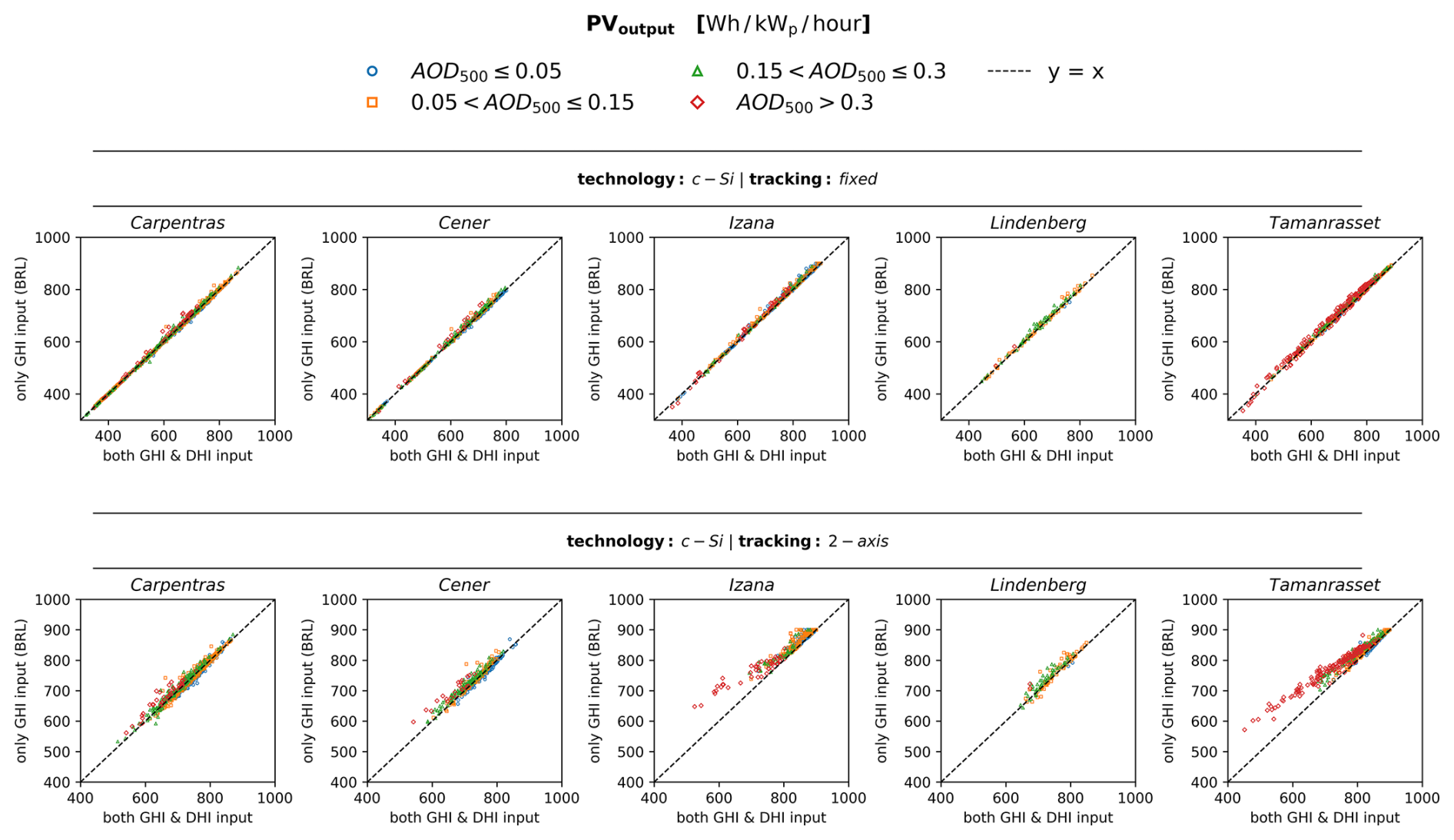
Figure 7 Comparison of the estimated hourly PV power generation between simulations performed using GSEE with input data consisting of either only GHI or both GHI and DHI under varying aerosol conditions: (top) fixed panels (bottom) 2-axis tracking systems.

The PV systems considered in this study have a nominal capacity of 1 kWp. The PV model applies a default system loss factor of 10 %. This effectively limits the maximum achievable power output to approximately 90 % of the nominal capacity (i.e., around 900 W kWp⁻¹). This effect becomes apparent at the Izaña site due to its low latitude combined with its specific geographical and atmospheric conditions, which lead to high irradiance levels. As a result, the simulated PV output in some cases appears capped around 900 Wh kWp⁻¹ per hour when only GHI is used.

Additionally, Tables 4 and 5 present the validation results for Carpentras and Tamanrasset, selected as representative locations that encompass a wide variety of sky conditions. Validation results for the remaining stations are available in the supplement (Tables S1–S3). All the evaluation metrics correspond to simulations of PV panels with c-Si technology.

Table 4 Evaluation metrics for GSEE performance within hourly intervals in Carpentras, comparing simulations with diffuse fraction from measurements and from the BRL model.

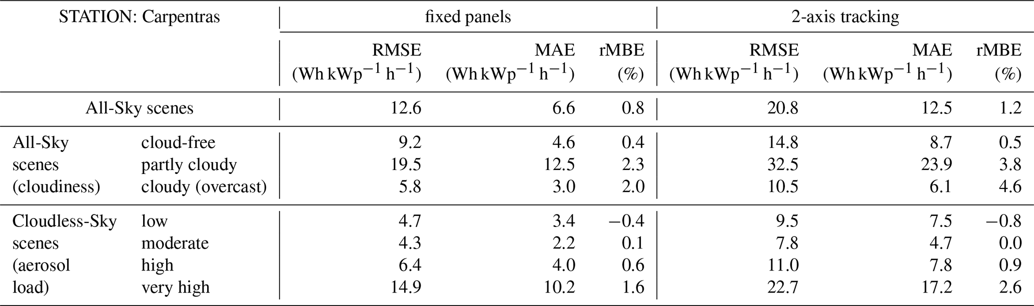
Table 5 Evaluation metrics for GSEE performance within hourly intervals in Tamanrasset, comparing simulations with diffuse fraction from measurements and from the BRL model.

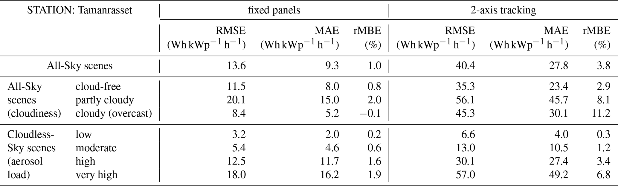
Based on the calculated statistical indices, the Root Mean Square Error (RMSE) values for fixed panels range from 4.7 Wh kWp⁻¹ h⁻¹ (clear sky) to 19.5 Wh kWp⁻¹ h⁻¹ (partly cloudy) in Carpentras, and from 3.2 to 20.1 Wh kWp⁻¹ h⁻¹ in Tamanrasset. Under very high aerosol loading, RMSE reaches 14.9 and 18.0 Wh kWp⁻¹ h⁻¹, respectively. For 2-axis tracking systems, RMSE values vary significantly, ranging from 9.5 to 32.5 Wh kWp⁻¹ h⁻¹ in Carpentras and from 6.6 to 56.1 Wh kWp⁻¹ h⁻¹ in Tamanrasset, with peaks of 22.7 and 57.0 Wh kWp⁻¹ h⁻¹ under very high aerosol loading conditions. Similarly, the Mean Absolut Error (MAE) values are generally lower for fixed panels (3.4–12.5 Wh kWp⁻¹ h⁻¹ in Carpentras, 2.0–15.0 in Tamanrasset) and substantially higher for 2-axis tracking (7.5–23.9 and 4.0–45.7 Wh kWp⁻¹ h⁻¹, respectively). Notably in Tamanrasset, MAE values under very high aerosol loading exceed those observed under partly cloudy conditions, with values increasing from 15.0 to 16.2 Wh kWp⁻¹ h⁻¹ for fixed panels and from 45.7 to 49.2 Wh kWp⁻¹ h⁻¹ for 2-axis tracking systems. Regarding the relative mean bias (rMBE), this remains mostly within ±4.6 % for fixed panels but can reach up to 11.2 % for 2-axis tracking, particularly in aerosol-laden conditions.

3.4 Estimating total daily PV power output using the Climate Interface

Validation of the estimated daily energy production using the Climate Interface is achieved by comparing the estimates with the results obtained from the direct summation of the hourly simulations with input both GHI and DHI.

The Climate Interface generates the hourly profile of GHI for each day as a sinusoidal function. Then, the BRL is applied to the hourly time-series, and the hourly power generation is computed. Finally, these values are summed up to provide an estimate of the total daily output power. As shown in Fig. 8, which illustrates the differences between the Climate Interface estimates and the sums of the hourly simulations, this approach introduces a variability throughout the year. Furthermore, Figure S6 in the supplement presents the percentage differences between the two approaches, using the latter as the reference.

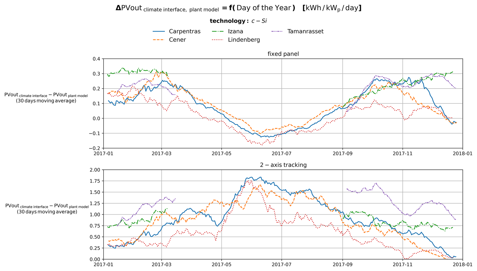
Figure 8 Time-series of the differences between the daily PV output estimated using the climate interface and the corresponding daily sums from hourly simulations.

The time-series represent the centered 30-day moving average. To ensure that the values are representative of the reference period, we have applied all conditions requiring at least 20 d of available data within each 30-days interval. In Tamanrasset and Izaña, especially during the summer months, there are significant data gaps on several days, often occurring around solar noon.

More precisely, from Fig. 8, we observe that within the modelling of PV plants with fixed panels, there is a tendency to overestimate in winter, with deviations of approximately 0.3 kWh kWp⁻¹ d⁻¹, and to slightly underestimate in summer, where deviations are around 0.1 kWh kWp⁻¹ d⁻¹. In contrast, for 2-axis solar tracking systems, the resulting deviations are significantly larger, with a general tendency toward overestimation that peaks during summer, reaching approximately 1.75 kWh kWp⁻¹ d⁻¹. The percentage differences span from −10 % to 20 % for fixed panels and from −5 % to 35 % for 2-axis tracking systems.

The variability in the percentage difference between the daily PV output estimated using the climate interface and the corresponding daily sums is mainly a function of the minimum SZA, while especially in the case of modeling for 2-axits tracking systems, the variation is also influenced by aerosol loading, with differences tending to increase as aerosol load rises (Figs. S4 and S5 in the Supplement).

Additional validation results are provided in the supplement (Tables S4–S8). Indicatively, for Carpentras and Tamanrasset, representative results are discussed below. For fixed panels, RMSE is minimized at 0.18 kWh kWp⁻¹ d⁻¹ under very-low aerosol conditions, compared to the overall 0.22 kWh kWp⁻¹ d⁻¹ for Carpentras. In Tamanrasset, the lowest RMSE is observed at 0.15 kWh kWp⁻¹ d⁻¹ under very low aerosol conditions, while the overall reaches 0.24. In the case of 2-axis tracking, a significant increase is observed from low-aerosol to aerosol-laden conditions, ranging from 0.82 to 1.28 kWh kWp⁻¹ d⁻¹ in Carpentras and from 0.66 to 1.37 in Tamanrasset. Similar widening trends are also evident in the MAE values across different aerosol loading conditions. The computed statistical indices confirm that the differences are minimized under sunny and nearly aerosol-free sky conditions. Comparing the performance on low-aerosol days to that on aerosol-laden, we conclude that, particularly in the case of modelling 2-axis tracking systems, errors increase significantly. In Tamanrasset, in particular, the errors are more than double.

3.5 Evaluation of the reliability of using the CAMS solar radiation time-series product in modelling PV power potential

The aim of this section is to inspect the reliability of using the CAMS solar radiation time-series product in modelling the PV power potential adapted to a certain location. A review of the existing literature indicates a lack of studies directly examining the accuracy of using CAMS data for assessing PV power potential. This is addressed by comparing the output power obtained from using CAMS solar radiation data with that calculated using ground-based measurements. The analysis focuses on the capability of CAMS to provide accurate estimates of both GHI as well as its individual components.

In this section, we have excluded Izaña, because, due to its high altitude – as indicated through a personal communication with Yves-Marie Saint-Drenan (2025) – comparable results would require adjusting the measurements to the elevation of the stations, which is a complicated process and beyond the scope of this study.

The CAMS-based diffuse fraction, compared to the observed, is presented in Fig. 9 under different prevailing conditions. We observe that the calculation of the diffuse component is subject to significant uncertainty. Cloudiness is the primary uncertainty source, particularly under partly cloudy conditions. Additionally, notable discrepancies related to aerosols emerge only in cases of very high aerosol loading.

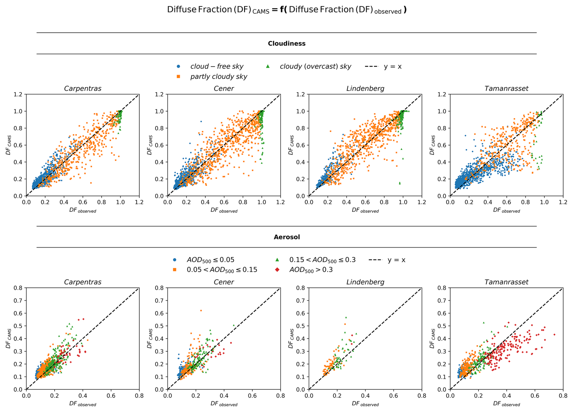
Figure 9 Comparison of the CAMS-based diffuse fraction estimated using BRL with the actual one under diverse atmospheric conditions.

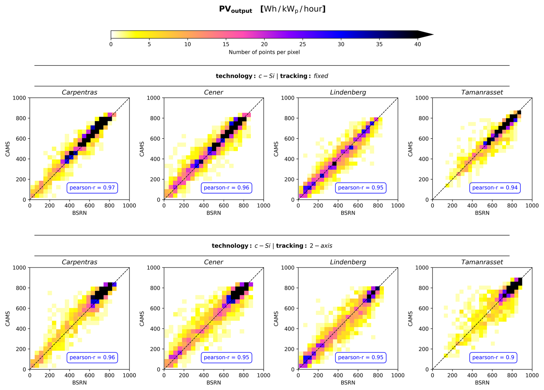
In Fig. 10 we provide density scatter plots comparing the CAMS-based PV output power with that computed from the ground-based BSRN data, aiming to illustrate how the uncertainty in the diffuse component estimates propagate to the calculation of power generation. Notably, there is a much greater dispersion from the y=x line in the case of simulating PV plants with 2-axis tracking system, compared to that within the modelling of fixed panels. This outcome is attributed to the increased sensitivity of the 2-axis tracking systems to the partitioning of global irradiance into its components. Nevertheless, correlation coefficients are in all cases better than 0.9.

Additional evaluation metrics are provided in the supplement (Tables S9–S12). Indicatively, we observe that under cloudless conditions, for fixed panels, RMSE ranges between 25.0 to 42.3 Wh kWp⁻¹ h⁻¹ in Carpentras and 16.6 and 31.0 Wh kWp⁻¹ h⁻¹ in Tamanrasset, with variations linked to aerosol loading. Similarly, MAE ranges from 20.0 to 36.9 Wh kWp⁻¹ h⁻¹ in Carpentras and 11.9 to 22.9 Wh kWp⁻¹ h⁻¹ in Tamanrasset. For 2-axis systems, RMSE and MAE follow similar trend, ranging from 28.8 to 49.9 Wh kWp⁻¹ h⁻¹ and 22.3 to 44.1 Wh kWp⁻¹ h⁻¹, respectively, in Carpentras, and from 20.8 to 48.0 Wh kWp⁻¹ h⁻¹ and 15.3 to 35.5 Wh kWp⁻¹ h⁻¹, respectively, in Tamanrasset. Conversely, under cloudy conditions the errors are significantly increasing. In Carpentras, as well as in Cener, and Lindenberg (according to the corresponding tables in the supplement) the errors peak under partly cloudy conditions, with RMSE reaching up to 94.2 Wh kWp⁻¹ h⁻¹ in Carpentras. However, in Tamanrasset, the highest errors occur under overcast conditions, where RMSE and MAE for 2-axis solar tracking systems reach 210.7 and 151.6 Wh kWp⁻¹ h⁻¹, respectively. This exception can be interpreted through Fig. 15, which illustrates that in the rare overcast scenes in Tamanrasset, CAMS occasionally reports low diffuse fraction values instead of values close to 1, suggesting that CAMS did not accurately represent cloudiness in these cases.

Figure 10 Overview of the reliability of the CAMS-based PV power simulations.

4 Conclusions

The optimal approach to include solar radiation information to PV power models such as GSEE is to use actual in-situ measurements of global and diffuse solar irradiance. Since measurements of the diffuse component are rarely available, it is common to use measurements of the GHI (if available) and retrieve the diffuse component using a model such as BRL. In the absence of in-situ measurements, other options include the use of datasets such as CAMS or even a radiative transfer model, provided that atmospheric inputs such as clearness index, aerosol optical depth (AOD), and other aerosol properties are available. This study evaluated these options and their implications for PV modelling accuracy.

The results highlighted the importance of having precise information for the distribution of solar irradiance among its components in PV power modelling. The implementation of the BRL diffuse fraction within GSEE serves as a practical, and under certain conditions, reliable solution to the absence of detailed information for each component separately. Moreover, the integrated Climate Data Interface submodule offers valuable prospects for investigating fluctuations in the solar PV power generation across various timescales. In this context, the use of BRL has a key contribution alongside the other computational procedures in processing climate datasets. Previous studies on PV power modelling approaches have not examined their reliability under diverse atmospheric conditions, including the effects associated with cloudiness, aerosol loading, as well as aerosol optical properties.

The evaluation of the BRL's performance revealed a dependency of its reliability on the prevailing sky conditions. BRL has excellent accuracy under totally clear sky scenes and still performs well for cloudless scenes with moderate aerosol loading. In general, its accuracy is inversely proportional to the complexity of the cloud scene. However, the model systematically underestimates the diffuse fraction under high-loading conditions, such as during dust events. The discrepancies arising from diffuse fraction estimation propagate to PV power generation and become particularly pronounced in the modelling of 2-axis tracking systems. Indicatively, MAE under cloud-free scenes with moderate aerosol loading, ranges between 2.2 to 6.6 Wh kWp⁻¹ h⁻¹ for fixed panels and 4.7 to 15.0 Wh kWp⁻¹ h⁻¹ for 2-axis tracking systems. Under partly cloudy conditions, where the cloud scene is more complex, the MAE increases substantially, ranging from 12.4 to 25.8 Wh kWp⁻¹ h⁻¹ for fixed panels and from 23.5 to 55.1 Wh kWp⁻¹ h⁻¹ for 2-axis tracking systems. Moreover, during intense dust events, MAE can reach up to 49.2 Wh kWp⁻¹ h⁻¹ in Tamanrasset, which is comparable to that computed under partly cloudy conditions. Overall, the rMBE remains within the ±5 %, with the exception of a limited cases under overcast conditions. The same analysis applied to CdTe panels yielded similar results, with minor differences.

Aiming to provide an indicative assessment of the financial impacts of the effect of desert dust aerosols, we assume that the statistical indices calculated for Tamanrasset are representative of a large-scale solar farm located in the Sahara region, with 500 MW installed PV capacity and systems equipped with 2-axis solar tracking system. For this hypothetical solar farm, according to the value of the Mean Absolute Error (MAE) on Table 4 for very high aerosol loading, we estimate that the produced energy is 0.0492 [Wh kWp⁻¹ h⁻¹] $\times \mathrm{500}\times {\mathrm{10}}^{\mathrm{3}}$ [kWp] =24 600 [kWh⁻¹ h⁻¹] $\stackrel{\mathrm{supposing}\mathrm{12}\mathrm{sunlight}\mathrm{hours}\mathrm{per}\mathrm{day}}{⟹}$ ∼295 200 [kWh d⁻¹] less than the expected from the PV power simulations. According to the global average auction prices for selling produced energy back to the grid in 2021 (IRENA, 2026), the overestimations are equivalent to a financial loss of 0.039 [USD/kWh] ×295 200 [kWh d⁻¹] ≈ USD 11 500 d⁻¹. Therefore, site assessments that do not correctly account for the distribution of surface solar irradiance in the sky under desert dust aerosol conditions may overestimate financial performance and the annual financial deficit could be accumulated to hundreds of thousands of US dollars per year.

Comparing the range of computed errors, we observe that the errors arising from employing CAMS rather than using ground-based measurements, even when the diffuse fraction is not provided, are higher across the overwhelming majority of the considered sky conditions. More specifically, regarding the overall performance, MAE when using CAMS ranges between 33.7 and 46.1 Wh kWp h⁻¹, while with ground-based GHI measurements, MAE remains below 10 Wh kWp h⁻¹ within the modelling of systems with fixed panels and can reach up to 27.8 Wh kWp h⁻¹ within the modelling of 2-axis tracking systems. This outcome highlights the value of ground-based measurements.

To sum up, achieving the highest quality PV power simulations necessitates high-quality, concurrent measurements of solar irradiance components. In absence of this, the submodules included in the GSEE package enable reliable simulations under the vast majority of prevailing sky conditions. CAMS serves as a valuable data source for PV power modelling, but it cannot fully replace the precision and reliability of using ground-based measurements. The integration of aerosol correction within the BRL model opens new possibilities for further improvements in the modelling of solar energy systems. A more comprehensive assessment would require measured PV output data; however, acquiring simultaneous direct and diffuse irradiance measurements at the same location as the solar farms remains challenging.