Optimal estimation retrieval framework for daytime clear-sky total column water vapour from MTG-FCI near-infrared measurements

A retrieval of total column water vapour (TCWV) from the new daytime, clear-sky near-infrared (NIR) measurements of the Flexible Combined Imager (FCI) onboard the geostationary satellite Meteosat Third Generation Imager (MTG-I, Meteosat-12) is presented. The retrieval algorithm is based on the differential absorption technique, relating TCWV amounts to the radiance ratio of a non-absorbing band at 0.865 µm and a nearby water vapour (WV) absorbing band at 0.914 µm. The sensitivity of the band ratio to WV amount increases towards the surface which means that the whole atmospheric column down to the boundary-layer moisture variability can be observed well.

The retrieval framework is based on an optimal estimation (OE) method, providing pixel-based uncertainty estimates. It builds on well-established algorithms for other passive imagers with similar spectral band settings. Transferring knowledge gained in their development onto FCI required new approaches. The absence of additional, adjacent window bands to estimate the surface reflectance within FCI's absorbing channel is mitigated using a principal component regression (PCR) from the bands at 0.51, 0.64, 0.865, 1.61, and 2.25 µm.

We utilize synergistic observations from Sentinel-3 Ocean and Land Colour Instrument (OLCI) and Sea and Land Surface Temperature Radiometer (SLSTR) to generate “FCI-like” measurements. OLCI bands were complemented with SLSTR bands, enabling evaluation of the retrieval's robustness and global performance of the PCR. Furthermore, this enabled algorithm testing under realistic conditions using well-characterized data, at a time when a long-term, fully calibrated FCI Level 1c dataset was not available. We built a forward model for two FCI equivalent OLCI bands at 0.865 and 0.9 µm. A long-term validation of OLCI against a single atmospheric radiation measurement (ARM) reference site without the PCR resulted in a bias of 1.85 kg m⁻², centred root-mean-square deviation (cRMSD) of 1.26 kg m⁻², and a Pearson correlation coefficient (r) of 0.995.

A first verification of the OLCI/SLSTR “FCI-like” TCWV against well-established ground-based TCWV products concludes with a wet bias between 0.33–2.84 kg m⁻², a cRMSD between 1.46–2.21 kg m⁻², and r between 0.98–0.99. In this set of comparisons, only land pixels were considered. Furthermore, a dataset of FCI Level 1c observations with a preliminary calibration was processed. The TCWV processed for these FCI measurements aligns well with reanalysis TCWV and collocated OLCI/SLSTR TCWV but shows a dry bias. A more rigorous validation and assessment will be done once a longer record of FCI data is available.

TCWV observations derived from geostationary satellite measurements enhance monitoring of WV distributions and associated meteorological phenomena from synoptic scales down to local scales. Such observations are of special interest for the advancement of nowcasting techniques and numerical weather prediction (NWP) accuracy as well as process-studies.

1 Introduction

Water vapour (WV) is the fundamental ingredient in the formation of clouds and precipitation. Spatio-temporal WV distributions and fluxes impact the intensity and duration of precipitation. The presence of sufficient low-level moisture in the atmospheric boundary layer facilitates the formation of convective development through the enhancement of atmospheric instability. Low-level moisture also contributes to storm severity by acting as a source of energy, once a storm has initiated (e.g. Johns and Doswell, 1992; Doswell et al., 1996; Fabry, 2006; Púčik et al., 2015; Peters et al., 2017). On a global, climatological scale, WV is a major contributor to global energy fluxes and, owing to its abundance and absorption over a wide range of the solar and terrestrial spectrum, acts as the strongest greenhouse gas (e.g. Trenberth et al., 2003; Schmidt et al., 2010). Within a changing climate, a warmer atmosphere will contain more WV, which may form a positive feedback loop and further enhance global warming. Moreover, a more moist atmosphere is predicted to produce more severe weather (e.g. Allen and Ingram, 2002; Neelin et al., 2022; Chen and Dai, 2023). But apart from that, WV is considered an inconvenient atmospheric component for several remote sensing applications for which precise information on WV amounts in the atmosphere are needed for atmospheric correction methods (e.g. Gao et al., 2009; Wiegner and Gasteiger, 2015; Valdés et al., 2021).

Observations of total column WV (TCWV) from satellite-based passive imagers operating in the visible (VIS), near-infrared (NIR) and thermal infrared (TIR) spectral ranges play a key role in monitoring its distribution at regional to global scales. WV retrievals using TIR measurements have a long history and are widely used, particularly from geostationary satellite platforms. On the one hand, a split-window technique using weakly absorbing WV measurements can be employed to retrieve TCWV or boundary-layer WV with relatively high uncertainties (e.g. Kleespies and McMillin, 1990; Casadio et al., 2016; Hu et al., 2019; Dostalek et al., 2021; El Kassar et al., 2021). Lindsey et al. (2014, 2018) showed that the split-window difference by itself may already provide valuable insight on the WV content in the boundary layer or lowest layers of the troposphere. On the other hand, measurements from strongly absorbing WV bands serve to retrieve WV amounts limited to upper tropospheric levels and/or layered WV products (e.g. Koenig and De Coning, 2009; Martinez et al., 2022). However, owing to the absorption and re-emission of radiation by WV in the infrared, such approaches rely on knowledge of the atmospheric temperature profile in addition to the atmospheric WV profile. Using observations in the VIS/NIR largely avoids these temperature-related complications.

The use of the so-called ρστ WV absorption region in the NIR (0.9 to 1.0 µm) is not new. This designation stems from the first observations of atmospheric absorption of solar radiation in the nineteenth century (Langley, 1902). Within the ρστ, light is more likely to be absorbed by WV molecules compared to spectral regions outside these absorption features (window regions). These NIR measurements exhibit the greatest sensitivity to WV amounts near the surface. Consequently, this allows for the retrieval of accurate clear-sky TCWV fields as well as providing information on changes of WV amounts in the lower troposphere. For several decades, the ρστ region has been researched using radiative transfer models and exploited in TCWV retrieval schemes (e.g. Fischer, 1988; Gao and J., 1992; Bennartz and Fischer, 2001; Albert et al., 2005; Lindstrot et al., 2012; Diedrich et al., 2015; Preusker et al., 2021). The focus first lay on ground-based radiometers and soon shifted to airborne and space-borne imagers. The first satellites that carried instruments with dedicated NIR WV bands were almost exclusively on satellite platforms with sun-synchronous, polar orbits and could deliver global daily coverage at hm to km resolution. Even at a km resolution, NIR TCWV can resolve convective phenomena such as horizontal convective rolls or gravity waves (Carbajal Henken et al., 2015; Lyapustin et al., 2014).

The new Meteosat Third Generation Imager (MTG-I, hereinafter referred to as MTG) carries the Flexible Combined Imager (FCI) (Holmlund et al., 2021; Martin et al., 2021). The European Organisation for the Exploitation of Meteorological Satellites (EUMETSAT) commissions this third generation of European geostationary meteorological satellites for monitoring weather and climate. FCI is the successor to the Spinning Enhanced Visible and Infrared Imager (SEVIRI) (Schmetz et al., 2002) and will enhance the temporal and spatial resolution of geostationary remote sensing observations. Also, an expanded set of spectral channels allows for more comprehensive observations of atmospheric and surface properties. FCI includes a new NIR WV absorption band not available on any other instrument onboard a geostationary platform to date. This band is located within the ρστ WV absorption region at 0.914 µm.

The introduction of MTG and its new FCI NIR band will expand our ability to quantify and characterize local to global-scale WV distributions and monitor their changes. This has important implications for both weather and climate research and applications. Particularly in the domain of nowcasting, FCI's fine-scale observation of TCWV could substantially advance the field (e.g. Benevides et al., 2015; Van Baelen et al., 2011; Dostalek et al., 2021). The Nowcasting and Very Short Range Forecasting Satellite Application Facility (NWCSAF) is an organization funded by EUMETSAT and aims to support meteorological services with satellite products critical for the prediction of high-impact weather (e.g. storms, fog). They commission, develop and maintain software which utilizes many weather satellite instruments, including MTG-FCI/Meteosat-12 (García-Pereda et al., 2019). A high-resolution NIR TCWV product in the portfolio of NWCSAF's software will greatly benefit the nowcasting and meteorological community at large.

In this work, we present our TCWV retrieval framework utilizing the novel NIR measurements obtained from MTG-FCI. Our approach builds on established TCWV retrieval frameworks successfully applied to other passive imagers sharing similar spectral band configurations. The differential absorption technique, using the ratio of measurements in the ρστ-absorption band and nearby window bands, was previously employed in measurements of the Medium Resolution Imaging Spectrometer (MERIS) onboard Envisat (Bennartz and Fischer, 2001; Lindstrot et al., 2012). With the launch of the Copernicus Sentinel-3A and Sentinel-3B satellites (Donlon et al., 2012) and onboard Ocean and Land Colour Imager (OLCI), the retrieval framework has been extended to fully exploit OLCI's extended spectral capabilities by using multiple bands sensitive to WV absorption (Preusker et al., 2021). Operational and calibrated FCI Level 1c data only became available at the end of 2024. Owing to the unique technical characteristics of FCI as well as the limited availability of a well-calibrated FCI data record at the time this work was conducted, new strategies are imperative for our methodology and its assessment. One key element is the surface reflectance approximation method for the absorption band, which can be assessed with the use of OLCI/SLSTR “FCI-like” data. In particular, we applied the same forward model and inversion principles to OLCI band 17 (0.865 µm) and band 19 (0.9 µm) as were used for FCI. The use of the OLCI/SLSTR synergy presents an excellent opportunity to establish an adapted retrieval framework and provides a robust test bed to explore algorithm performance accordingly. In addition, OLCI Level 1b has well-known radiometric characterization and worldwide coverage, allowing for a practical and reliable basis to assess and refine the retrieval framework under a wide range of realistic atmospheric and surface conditions.

The structure of this paper is as follows: in Sect. 2, we introduce the FCI data, OLCI/SLSTR data, auxiliary data, and the TCWV reference datasets, along with the associated matchup method. The FCI TCWV algorithm, covering the physical background, forward model, inversion method, and the albedo approximation method integral to the algorithm, as well as the finalized retrieval framework are presented in Sect. 3. In Sect. 4, we present the results of the matchup assessments conducted on both local and global scales, along with initial analyses using a preliminary calibrated FCI dataset and a representative case study. The discussion and outlook are given in Sect. 5. Finally, in Sect. 6, we conclude the paper.

2 Data

2.1 MTG-FCI data

MTG is an operational EUMETSAT satellite mission, which currently consists of one satellite in geosynchronous orbit at 0° longitude. It carries the Lightning Imager (LI) and the FCI which is a multispectral instrument that scans with a fast east-west and a slow north-south motion. It has 16 bands which range from the VIS (0.44 µm) to the TIR (13.3 µm). The full disc scan service covers approximately one-fourth of the Earth's surface within 10 min, covering Europe, Africa, and parts of the Atlantic and Indian oceans (Durand et al., 2015; Holmlund et al., 2021). In the future, a second FCI will provide a rapid scan service, which covers the northern third of the full disc within 2.5 min, covering parts of Europe and the Mediterranean. The spatial resolution at sub-satellite point (SSP) of one VIS band at 0.64 µm and one SWIR band at 2.25 µm is 0.5 km. The spatial resolution of the other VIS to SWIR bands and the TIR bands at 3.8 and 10.5 µm is 1.0 km at SSP. The remaining TIR bands have an SSP resolution of 2.0 km. Owing to the curvature of the Earth, the actual spatial resolution outside the SSP is slightly lower. For example, the 1 km SSP resolution (VIS, NIR and 10.5 µm) in Northern Europe is closer to 2.0 to 3.0 km.

The first MTG satellite was launched successfully into orbit on 13 December 2022 and has left the commissioning phase in December 2024. Work on this algorithm concluded in November 2024. Because of that, we used the latest release of preliminary FCI Level 1c data at the time provided by EUMETSAT in February 2024 (EUMETSAT, 2024b). They consist of one full disc scene from 13 January 2024 between 11:50 and 12:00 UTC. They were downloaded from EUMETSAT's SFTP server and more details on this dataset can be found in EUMETSAT (2024a). At the time of publication, no cloud mask was available for the FCI test data. Therefore, we built a simple cloud mask algorithm. The cloud masking algorithm is largely based on the work presented in Hünerbein et al. (2023). In this publication, the authors adapted and extended cloud masking and typing algorithms developed for NASA's Aqua/Terra Moderate Imaging Spectrometer (MODIS) (Ackerman et al., 2002) to ESA's Cloud Aerosol and Radiation Explorer Mission (EarthCARE) Multi Spectral Imager (MSI). We adapted a subset of their tests to the FCI bands and estimated new coefficients and thresholds. Ultimately, the cloud mask consists of two tests: threshold tests for reflectances, a reflectance ratio or the Global Environmental Monitoring Index (GEMI) (Pinty and Verstraete, 1992).

2.2 S3-OLCI/SLSTR data

Sentinel-3 is an operational COPERNICUS satellite mission of the European Commission, managed by EUMETSAT. It consists of two sister satellites (Sentinel-3A: S3A; Sentinel-3B: S3B) which orbit the Earth at an altitude of 814.5 km, an inclination of 98.65° and a local Equator crossing time of 10:00 am UTC. S3B is phase-shifted to S3A by 140°. This way, the imaging instruments onboard the two satellites achieve global coverage almost daily. The payloads consist of OLCI, the Sea and Land Surface Temperature Radiometer (SLSTR) and the Synthetic Aperture Radar Altimeter (SRAL), supported by the Microwave Radiometer (MWR).

OLCI is a push-broom multispectral imaging spectrometer that consists of five cameras. It measures at 21 bands ranging from the VIS (0.4 µm) to the NIR (1.02 µm). The swath width of OLCI is 1215 km at a full SSP resolution of 0.3 km per pixel, which is referred to as “Full Resolution”. In the “Reduced Resolution”, 4 by 4 pixels are aggregated into 1.2 km pixels. That is the resolution used in this study. A characteristic of OLCI is an across-track spectral shift owing to the five discrete cameras. This can be corrected for by taking into account the actual central wavelength at each of the across-track pixels (Preusker, 2025). To replicate the capabilities of FCI at a similar spatial resolution and with similar spectral characteristics, we collocated SLSTR observations to the OLCI grid using nearest-neighbour sampling. The SLSTR bands used are S5 (1.612 µm, 0.5 km) and S6 (2.25 µm, 0.5 km). They have been mapped to OLCI's reduced resolution at 1.2 km. Using Sentinel-3A and B, a representative set of swaths was created for every month of the year 2021 which amounts to a total of 1800 swaths across 80 d. The Identification of Pixel features (IdePIX) cloud detection algorithm was used to create cloud masks (Iannone et al., 2017; Wevers et al., 2021; Skakun et al., 2022).

2.3 ECMWF ERA5 forecast and reanalysis data

Our TCWV retrieval is based on an inversion technique (Sect. 3) which uses a first guess, as well as a priori and ancillary parameter data. These may come from a climatology or could be set to a global climatological value. However, retrieval performance can be greatly increased and sped up if the a priori data are already slightly closer to the solution. This is why we chose to provide the algorithm with numerical weather prediction (NWP) forecast fields. These were acquired from the European Centre for Medium-Range Weather Forecasts (ECMWF) ERA5 forecasts initialized at 06:00 and 18:00 UTC of each day (Hersbach et al., 2020). The ERA5 forecasts are a byproduct of the reanalysis and more readily available for past time steps than the operational forecasts. They are different from ECMWF's Integrated Forecasting System (IFS) operational forecasts since they use more assimilated data in the initialization time step. The forecasts are at a resolution of 0.25° and in 3 h steps. The data fields are interpolated to the observation time and FCI coordinates.

The variables needed are: horizontal wind speed (WSP) calculated from u- and v-component of the horizontal wind speed at 10 m above ground (U10, V10), TCWV, surface air temperature at 2 m above ground (T_2 m), and surface air pressure (SP). The data were accessed via the Copernicus Climate Change (C3S) data store (Copernicus Climate Change Service and Climate Data Store, 2023). For testing and algorithm development, we used the ERA5 forecasts. In the later processing for the NWCSAF GEO software package, the operational ECMWF IFS forecasts at a resolution of 0.5° and 1 h steps were used.

2.4 Aerosol optical thickness climatology

One key parameter for the retrieval of TCWV over water is the aerosol optical thickness (AOT). As a first guess for AOT, we use a climatology at a 1° spatial resolution. It was built from monthly means of the Oxford-Rutherford Appleton Laboratory Aerosol and Cloud (ORAC; Thomas et al., 2009) AOT dataset retrieved with SLSTR and the Environmental Satellite (ENVISAT) Advanced Along Track Scanning Radiometer (AATSR) between 2002 and 2022. These data were also accessed via the C3S data store (Copernicus Climate Change Service and Climate Data Store, 2019).

2.5 Reference datasets, matchup analysis, and performance indicators

To verify the credibility of the retrieved TCWV, we need reference data within the field of view of FCI. There are four established sources of TCWV estimates: radiosondes, ground-based GNSS meteorology, ground-based MWR, and ground-based direct sun-photometry. TCWV from NWP reanalyses may also be used, but their coarse resolution cannot resolve the fine variabilities found in the WV field at the satellite-pixel scale. Reanalyses may be used to assess the stability of the dataset later on. Unfortunately, until the completion of this work, no long-term record of FCI data was available in the final calibration. Because of this, we processed the spectrally representative FCI data discussed above and compared these against TCWV from the ERA5 reanalysis. The performance of our algorithm and the accuracy of our calculations require testing on real data. Hence, we processed a 7-year matchup database of OLCI Level 1b observations and MWR TCWV from the Southern Great Plains site of the atmospheric radiation measurement network (ARM) (Sisterson et al., 2016). In addition, the set of 1800 OLCI/SLSTR swaths was processed with our algorithm (including the surface reflectance approximation from Sect. 3.4). These were compared against reference TCWV data retrieved at sites of (1) the Aerosol Robotic Network (AERONET) (Holben et al., 1998), (2) the ARM network (Turner et al., 2007; Cadeddu et al., 2013) and (3) the SUOMINET network (Ware et al., 2000).

Prior to the analysis, OLCI swaths and ground-based network sites were collocated within 1 km and 30 min of a satellite overpass. A square of 11 by 11 pixels around the collocated centre pixel was taken into account. Then, these pixels were screened for convergence, a cost-function below 1, and cloud-screened with a buffer of 3 pixels around the cloud mask, minimizing the effect of cloud and cloud shadow contamination. Matchup cases with less than 95 % valid pixels were rejected, the central 3 by 3 pixels had to be completely cloud-free.

Both in the assessment of assumptions and the assessment of TCWV quality, we used metrics. Their abbreviations are as follows: N is the number of matchups, MADP is the mean absolute percentage deviation, RMSD is the root-mean-square deviation, cRMSD is the centred RMSD (i.e. the observation is corrected for the bias against the reference), r is the Pearson correlation coefficient. ODR α and β are the orthogonal distance regression coefficients for the intersect and slope, respectively, with equal weights for all data points.

3 Algorithm description

3.1 Physical background

The ρστ WV absorption bands are due to the vibrational reaction in a gaseous water molecule hit by a photon within a specific range of wavelengths, see Fig. 1. The absorption of WV in this spectral region is weak compared to the TIR at, e.g. 6.7 or 7.3 µm (traditionally referred to as WV bands). Because of that, the whole column's content of atmospheric WV can be probed using the ρστ. While the signal within the absorption band decreases with WV content, an adjacent window band will be virtually unaffected by any change in WV amount along the line-of-sight. FCI features a “window” band with a nominal centre wavelength of 0.865 µm and an “absorption” band with a nominal centre wavelength of 0.914 µm. The spectral response functions (SRF) are also shown in Fig. 1.

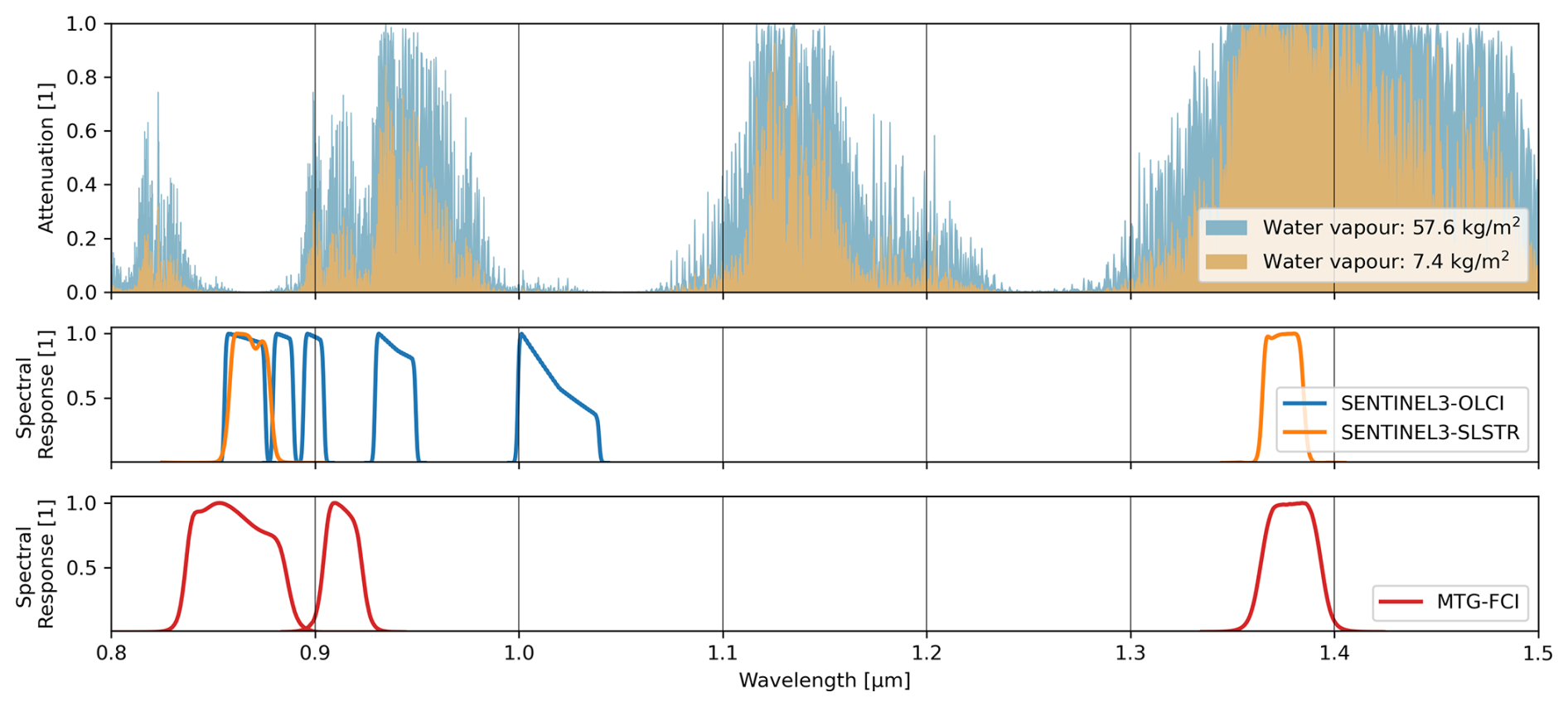
Figure 1 Upper panel: The WV attenuation spectrum for an atmosphere with a low TCWV amount in orange (7.4 kg m⁻²) and high TCWV amount in blue (57.6 kg m⁻²) with data obtained from the Correlated K-Distribution Model Intercomparison Project (CKDMIP; Hogan and Matricardi, 2020). Centre panel: The SRFs in the NIR part of the spectrum for the satellite instruments OLCI (blue) and SLSTR (orange). Lower panel: the SRFs in the NIR for FCI (red).

The overall strongest influence factor on the signal measured at the satellite sensor is the surface reflectance. This is also referred to as the surface spectral albedo (ALB) and is the ratio of outgoing irradiance against incoming irradiance at one specific wavelength. This ratio depends on the type of surface covering (e.g. vegetation, sand, snow, etc.) and to some degree on the sun and viewing angles. For land cases, the spectral albedo in the NIR is well above 0.3 and thus provides a strong signal relative to the absorption by WV. Over the majority of water surfaces, however, the surface reflectance is often well below 0.03. There is no direct way to measure this spectral albedo, hence an approximation is necessary.

A slightly less important effect comes from scattering aerosol layers below a certain level of AOT. In that case, the effective line-of-sight is shortened by the higher aerosol layer, and since the humidity content on average is much lower in the higher troposphere, the absorption is decreased substantially. Over bright surfaces, this effect is much less influential than over dark surfaces (Lindstrot et al., 2012). Since most natural surfaces over land are bright in the NIR, the shielding effect of an average aerosol layer is small (Diedrich et al., 2015).

Under most circumstances, this assumption is not valid for water surfaces, though. Owing to the low albedo, already slightly scattering layers of aerosol may create the effect described above. To a certain degree, this effect can be corrected for by simulating an aerosol layer with a specific AOT in the algorithm. However, for this, the effective height of the aerosol layer needs to be estimated, which is a challenge in and of itself. Another important aspect over water surfaces is sunglint, i.e. the reflectance's dependency on wind-speed and viewing/solar geometry. High wind speeds create a rough surface with low reflectance peaks spread out over a range of observation geometry angles. At lower wind speeds, a calm surface results in a higher reflectance peak over a limited range of observation angles, similar to a mirror. In regions with strong sunglint, the relative influence of aerosol scattering is reduced.

Over both land and water surfaces, the atmospheric temperature profile and surface pressure play a lesser role owing to temperature- and pressure-dependent line broadening (Rothman et al., 1998). In contrast to TCWV retrievals in the TIR, the impact of the temperature profile is substantially lower but not negligible. The uncertainties owing to a mis-characterized temperature profile are approximately 0.6 kg m⁻² and surface pressure at about 0.9 kg m⁻² (Lindstrot et al., 2012).

3.2 Forward model

The first step in our framework is to run radiative transfer simulations for a set of complete and comprehensive atmospheric, surface and geometric conditions as described in the previous section and listed in Tables 1 and 2. For the simulation of top-of-atmosphere (TOA) reflectances we used the Matrix Operator Model (MOMo; Fell and Fischer, 2001; Hollstein and Fischer, 2012; Doppler et al., 2014). These simulations are then sorted into two look-up-tables (LUT) for land surfaces and water surfaces, respectively.

Table 1 Land surface set-up for MOMo.

^∗ Standard profiles from Anderson et al. (1986).

Table 2 Water surface set-up for MOMo.

^∗ Standard profiles from Anderson et al. (1986).

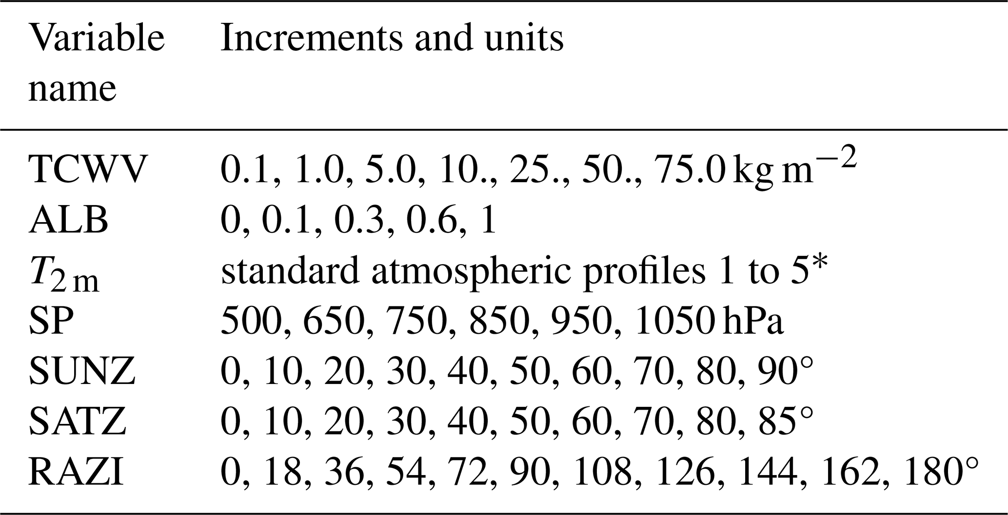
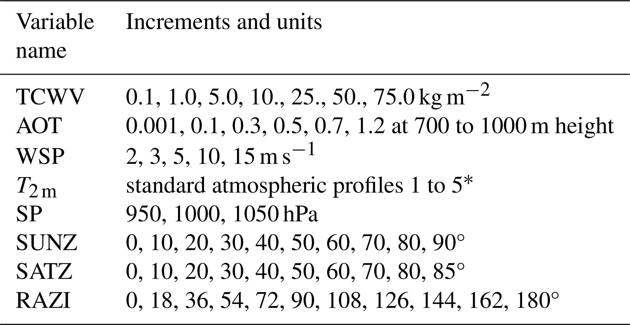
Over land surfaces, the surface albedo (ALB) is defined as isotropic. Over water surfaces, the surface reflectance is estimated from the 10 m wind speed (WSP) using Cox and Munk (1954). Standard atmospheric profiles were taken and adapted from Anderson et al. (1986) to provide the vertical distribution of temperature and humidity. The numbers refer to: 1 – mid-latitude summer, 2 – mid-latitude winter, 3 – sub-Arctic summer, 4 – sub-Arctic winter, 5 – tropical. Based on the forecast surface air temperature (T_2 m) and surface pressure (SP) the associated atmospheric profile group is chosen. The humidity profiles are scaled with TCWV. All simulations are done for a set of satellite zenith angles (SATZ), sun zenith angles (SUNZ) and relative azimuth (RAZI). RAZI is calculated from the satellite azimuth angle (SATA) and sun azimuth angle (SUNA) following

$$\begin{array}{}\text{(1)}& \begin{array}{rl}\mathrm{RAZI}=& \arccos \left(\cos \left(\mathrm{SUNA}\right)\cdot \cos \left(\mathrm{SATA}\right)\right.\\ & \left.+\sin \left(\mathrm{SUNA}\right)\cdot \sin \left(\mathrm{SATA}\right)\right).\end{array}\end{array}$$

The aerosol mixtures and their optical properties have been calculated using the OPAC software package (Optical Properties of Aerosols and Clouds; Hess et al., 1998). Within their documentation, one can find details on the used aerosol mixtures for the two types selected for the land and water surface simulations. Over land, we used the aerosol mixture “continental average”, over ocean we used the aerosol mixture “maritime clean”. In both cases, we simulated a homogenous aerosol layer between 700 and 1000 m height above ground with the specified AOT. Overviews of the inputs and increments used for the simulations are listed in Tables 1 and 2.

The observations we simulate are the normalized radiance in the window channel (nL_TOA(0.865 µm)) and the pseudo optical thickness in the absorption channel (τ_pTOA(0.914 µm)). The normalized radiance is calculated as follows:

$$\begin{array}{}\text{(2)}& {\mathrm{nL}}_{\mathrm{TOA}}\left(\mathit{\lambda }\right)={\displaystyle \frac{L_{\mathrm{TOA}}\left(\mathit{\lambda }\right)}{F_{\mathrm{0}}\left(\mathit{\lambda }\right)}},\end{array}$$

where F₀ is the spectral solar irradiance.

The pseudo optical thickness τ_pTOA is calculated as follows:

$$\begin{array}{}\text{(3)}& {\mathit{\tau }}_{\mathrm{pTOA}}\left(\mathit{\lambda }\right)=-a-{\displaystyle \frac{\log \left(\frac{{\mathrm{nL}}_{\mathrm{TOA}}\left(\mathit{\lambda }\right)}{{\mathrm{nL}}_{\mathrm{TOA}}^{*}\left(\mathit{\lambda }\right)}\right)}{\sqrt{\mathrm{AMF}}}}\cdot b,\end{array}$$

where AMF is the air mass factor, ${\mathrm{nL}}_{\mathrm{TOA}}^{*}$ is the normalized radiance corrected for the influence of WV absorption, and a and b are the so-called correction coefficients which may correct for a systematic bias discovered in a validation against reference TCWV observations.

The AMF is calculated as follows:

$$\begin{array}{}\text{(4)}& \mathrm{AMF}={\displaystyle \frac{\mathrm{1}}{\cos \left(\mathrm{SUNZ}\right)}}+{\displaystyle \frac{\mathrm{1}}{\cos \left(\mathrm{SATZ}\right)}}.\end{array}$$

The division of $-\log \left(\frac{{\mathrm{nL}}_{\mathrm{TOA}}\left(\mathit{\lambda }\right)}{{\mathrm{nL}}_{\mathrm{TOA}}^{*}\left(\mathit{\lambda }\right)}\right)$ by $\sqrt{\mathrm{AMF}}$ results in a more linear relationship between τ_pTOA and TCWV. This reduces the number of necessary iterations later on. ${\mathrm{nL}}_{\mathrm{TOA}}^{*}$ needs to be approximated using other available information (e.g. a climatology atlas, neighbouring window channels). Here, we use a more elaborate technique, described in Sect. 3.4.

Preusker et al. (2021) obtained the correction coefficients a and b by minimizing the differences between simulated and measured OLCI observations using ARM-SGP.C1-MWR TCWV as an input (see Preusker et al., 2021 for details). For OLCI's version of this algorithm, a and b for band 19 (at 0.9 µ m) were estimated to be −0.008 and 0.984, respectively, from the results shown in Sect. 4.1. For FCI, other MWR TCWV references will be necessary. We intend to use reference sites such as Meteorological Observatory Lindenberg – Richard Assmann Observatory (MOL–RAO) (Knist et al., 2022), the Cabauw Experimental Site for Atmospheric Research (CESAR) (Van Ulden and Wieringa, 1996) or ARM – Eastern North Atlantic (ENA) (Mather and Voyles, 2013).

The set of simulations is sorted into a multidimensional LUT. This LUT can then be used to simulate a measurement (y) for a given set of states (x) and parameters (p) using an interpolator. This is referred to as the forward model F. With this forward model, we can estimate a sensor's observation for a given set of states as follows:

$$\begin{array}{}\text{(5)}& \mathit{y}=\mathbf{F}(\mathit{x},\mathit{p})+\mathit{ϵ},\end{array}$$

where ϵ denotes the measurement and forward model error. The state vector of land consists of TCWV and ALB(0.865 µm), over water surfaces it consists of TCWV, WSP, and AOT. The parameter vector is composed of T_2 m, SP, SUNZ, SATZ, and RAZI.

3.3 Inversion using optimal estimation

Equation (5) can be inverted to retrieve a state associated with an observation. There are various ways of performing this inversion. We chose to follow the optimal estimation (OE) approach for atmospheric inverse problems described by Rodgers (2000). In essence, this inversion is based on the principle of minimizing the cost function J by iteratively changing the initial first guess of a state or the state of the prior iteration step.

The iterative process is stopped if either the maximum number of allowed steps is reached or the following criterion is met by the retrieved state x_i+1:

$$\begin{array}{}\text{(6)}& {\left({\mathit{x}}_i-{\mathit{x}}_{i+\mathrm{1}}\right)}^T{\widehat{\mathbf{S}}}_i^{-\mathrm{1}}\left({\mathit{x}}_i-{\mathit{x}}_{i+\mathrm{1}}\right)\le n\cdot \mathit{ϵ},\end{array}$$

where $\widehat{\mathbf{S}}$ is the retrieval error-covariance and n is the number of state variables. More details on the process of OE within a TCWV retrieval framework can be found in Preusker et al. (2021) and El Kassar et al. (2021). One crucial advantage of OE is the simultaneous retrieval of the associated uncertainty, the so-called retrieval error covariance matrix $\widehat{\mathbf{S}}$:

$$\begin{array}{}\text{(7)}& \widehat{\mathbf{S}}={\left({\mathbf{S}}_{\mathrm{a}}^{-\mathrm{1}}+{\mathbf{K}}_i^T\cdot {\mathbf{S}}_{\mathit{ϵ}}^{-\mathrm{1}}\cdot {\mathbf{K}}_i\right)}^{-\mathrm{1}},\end{array}$$

where, S_a is the a priori error covariance matrix associated with x_a, S_ϵ is the measurement error covariance matrix associated with y, and K is the Jacobian which contains the partial derivatives of each measurement to each state at step i (i.e. ${\mathbf{K}}_i=\partial \mathbf{F}\left({\mathit{x}}_i\right)/\partial {\mathit{x}}_i$). The covariances may be set to values that correspond to the actual covariances within a given variable. However, the covariances may also be used as tuning parameters to make the algorithm lean more towards the measurement or more towards the prior knowledge (Rodgers, 2000). Over land surfaces we set the a priori uncertainty of TCWV very high (16 kg m⁻²) since the information content of the absorption band is high over bright surfaces. Over the ocean, the TCWV a priori uncertainty was set much lower (2.5 kg m⁻²). The ALB a priori uncertainty is set to 0.5, the WSP a priori uncertainty is set to 5 m s⁻¹, and the AOT a priori uncertainty is set to 0.55. The corresponding covariances are the squared uncertainties.

The error covariance of τ_pTOA is estimated using the signal-to-noise-ratio (SNR), the interpolation-error from the uncertainty in estimating ${\mathrm{nL}}_{\mathrm{TOA}}^{*}$ (ϵ_intp), and the AMF:

$$\begin{array}{}\text{(8)}& {\mathbf{S}}_{\mathit{ϵ}}\left({\mathit{\tau }}_{\mathrm{pTOA}}\right)=\left({\displaystyle \frac{\mathrm{1}}{{\mathrm{SNR}}^{\mathrm{2}}}}+{\displaystyle \frac{\mathrm{1}}{{\mathrm{SNR}}^{\mathrm{2}}}}+{\mathit{ϵ}}_{\mathrm{intp}}^{\mathrm{2}}\right)\cdot {\displaystyle \frac{\mathrm{1}}{\mathrm{AMF}}}.\end{array}$$

In Eq. (8), the two SNR-terms refer to the uncertainty of nL_TOA(0.914 µm) and ${\mathrm{nL}}_{\mathrm{TOA}}^{*}$(0.914 µm). For nL_TOA(0.865 µm) the error covariance is simply $\frac{\mathrm{1}}{{\mathrm{SNR}}^{\mathrm{2}}}$.

An additional metric this inversion technique provides is the so-called averaging kernel A:

$$\begin{array}{}\text{(9)}& \mathbf{A}=\mathbf{G}\cdot \mathbf{K}={\displaystyle \frac{\partial \widehat{\mathit{x}}}{\partial \mathit{x}}},\end{array}$$

where G is the Gain matrix, which contains the partial derivative of the true state $\partial \widehat{\mathit{x}}$ in relation to the partial derivative of the measurement ∂y. While the true state $\widehat{\mathit{x}}$ is unknown, the relative changes at each step quantify the sensitivity of $\widehat{\mathit{x}}$ towards changes in y.

The entries along the diagonal of A correspond to the state variables and show a range of values between 0 and 1. At 0, the proportion of the retrieved state to $\widehat{\mathit{x}}$ is lowest; the measurement did not contribute to the retrieval. At 1, the proportion of the retrieved state to the true state is highest. Everything in between indicates that some improvement of the prior information about the state could be made using the measurement. The trace of AVK gives the degrees of freedom of the measurements.

3.4 Estimation of ${\mathrm{nL}}_{\mathrm{TOA}}^{*}$ with principal component regression

For some surfaces (e.g. calm, clear water), the difference in spectral albedo between the window and absorption channel is small. Over most other surfaces, however, this is not the case. Simply using nL_TOA(0.865 µm) for ${\mathrm{nL}}_{\mathrm{TOA}}^{*}$ would yield an unreliable estimate of the pseudo optical depth τ_pTOA. Thus, in order to calculate τ_pTOA we need an accurate estimate of the spectral slope between the window and the absorption channel. For satellite sensors such as MODIS or OLCI, the WV absorption bands have at least two accompanying window bands (i.e. at 0.865, 0.885, 1.02, or 1.2 µm). FCI and other future instruments do not have such additional window channels close by. Hence, another technique to estimate the spectral slope is needed.

The principal component regression (PCR) facilitates the reconstruction of a continuous set of observations from few discrete data points. This approach is already used with reasonable success in the estimation of BRDFs and reflectance spectra within RTTOV (Vidot and Borbás, 2014). Their approach was used as a blueprint for our spectral slope estimation.

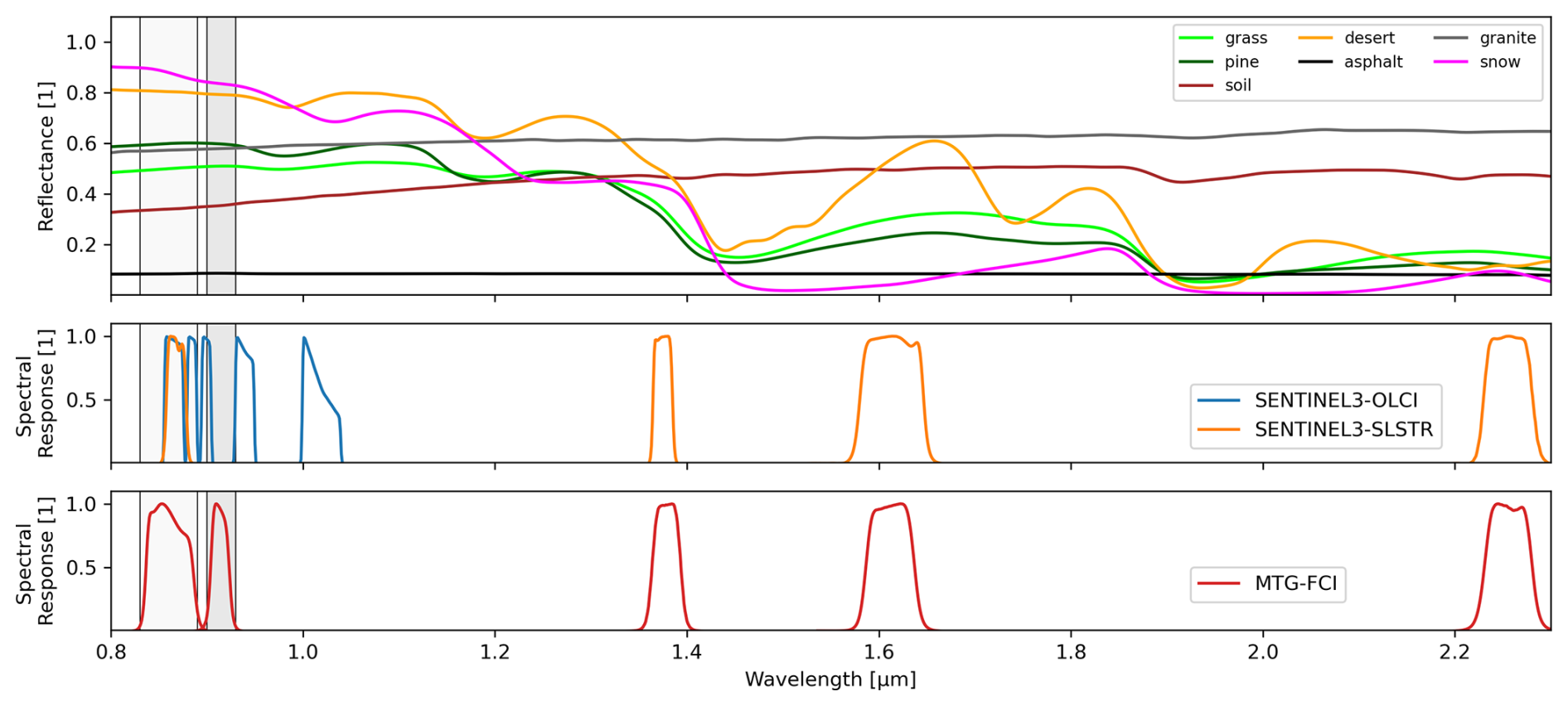
Figure 2 Upper panel: overview of a selection of surface reflectance spectra from Meerdink et al. (2019), the labels are representative and not the actual spectra designations. Central panel: the SRFs of OLCI (blue) and SLSTR (orange). Lower panel: the SRFs of FCI (red).

The ECOSTRESS spectral library version 1.0 provided by the United States of America Geological Service (USGS) is a collection of spectral reflectances for individual materials and/or mixtures at a high spectral resolution (Meerdink et al., 2019). The library consists of spectra for a wide range of material groups: human-made, rock, soil, mineral, photosynthetic vegetation, non-photosynthetic vegetation, and water (which includes fresh-water, ice, and snow). A small selection of these spectra is depicted in the upper part of Fig. 2. In the lower two panels of Fig. 2, the SRFs of a selection of sensors are shown.

Only spectra between 0.4 and 2.35 µm were taken into account and linearly interpolated to a spectral resolution of 0.001 µm. To avoid a sampling bias towards a specific group of spectra, we used similarly sized subsets of each category. From this database, the principal components (the eigenvectors, PCs) are calculated and sorted by their associated eigenvalue. Instead of reconstructing spectrally high-resolution reflectances, we use the PCs to reconstruct the reflectance of two channels: at 0.865 and at 0.914 µm, referred to as the target. Following the nomenclature of Vidot and Borbás (2014), R_target is the vector of reflectance spectra folded to the target SRFs, c_win is the regression coefficient vector (also referred to as weights) from the window bands, and U_target is the matrix of the selected PCs of the high-resolution reflectance spectra, folded to the target SRFs:

$$\begin{array}{}\text{(10)}& {\mathit{R}}_{\mathrm{target}}={\mathit{c}}_{\mathrm{win}}{\mathbf{U}}_{\mathrm{target}}.\end{array}$$

Using the Moore–Penrose Pseudo inverse, the regression coefficient c_win follows:

$$\begin{array}{}\text{(11)}& {\mathit{c}}_{\mathrm{win}}={\mathit{R}}_{\mathrm{win}}{\mathbf{U}}_{\mathrm{win}}^T{\left({\mathbf{U}}_{\mathrm{win}}{\mathbf{U}}_{\mathrm{win}}^T\right)}^{-\mathrm{1}}.\end{array}$$

An optimal configuration of the number of PCs and bands was then found by comparing different band combinations with several numbers of PCs. To do this, we reconstructed all available spectra at the target bands which were used in the PCR from the folded spectra at the window bands. Using this approach, the optimal configuration for FCI was found with the use of five window bands (i.e. negligible WV attenuation) in the VIS to SWIR (0.51, 0.64, 0.865, 1.61, 2.25 µm) and only the first four PCs. We are able to reproduce the actual surface reflectance at the absorption and window band with a bias of 0.0045 and 0.0038 and RMSD of 0.016 and 0.02, respectively. Folding the PCs to the SRFs of other sensors would make this matrix applicable to other instruments with similar bands, as shown in Fig. 2. To estimate the spectral slope in the PCR, FCI's normalized radiances at the window channels need to be transformed into irradiance reflectances:

$$\begin{array}{}\text{(12)}& {\mathit{\rho }}_{\mathrm{TOA}}\left(\mathit{\lambda }\right)={\displaystyle \frac{{\mathrm{nL}}_{\mathrm{TOA}}\left(\mathit{\lambda }\right)\cdot \mathit{\pi }}{\cos \left(\mathrm{SUNZ}\right)}}.\end{array}$$

From the reconstructed surface reflectances, we calculate the slope S:

$$\begin{array}{}\text{(13)}& S={\displaystyle \frac{\mathit{\rho }\left(\mathrm{0.914}\right)}{\mathit{\rho }\left(\mathrm{0.865}\right)}}.\end{array}$$

This ratio is then multiplied with the nL_TOA(0.865 µm) to yield a more accurate estimate of ${\mathrm{nL}}_{\mathrm{TOA}}^{*}$ at the absorption band. The underlying assumption is that between 0.865 and 0.914 µm, atmospheric scattering and attenuation other than WV are nearly identical. Thus, $\frac{\mathrm{ALB}\left(\mathrm{0.914}\right)}{\mathrm{ALB}\left(\mathrm{0.865}\right)}\approx \frac{{\mathit{\rho }}_{\mathrm{0}\mathrm{TOA}}\left(\mathrm{0.914}\right)}{{\mathit{\rho }}_{\mathrm{0}\mathrm{TOA}}\left(\mathrm{0.865}\right)}$ holds true. Given a sufficiently bright surface and outside the influence of thick, scattering layers (e.g. clouds, aerosols), or very slant viewing geometries (SATZ>82°), this is the case. Over water surfaces, the influence of scattering processes in the atmosphere is much stronger. Hence, the uncertainties over water pixels are higher. Furthermore, the influence of water constituents (e.g. sediment, pigments) on the water reflectance spectrum in the NIR has not been taken into consideration. The PCA training dataset almost exclusively consisted of terrestrial reflectances and only a few fresh water reflectances.

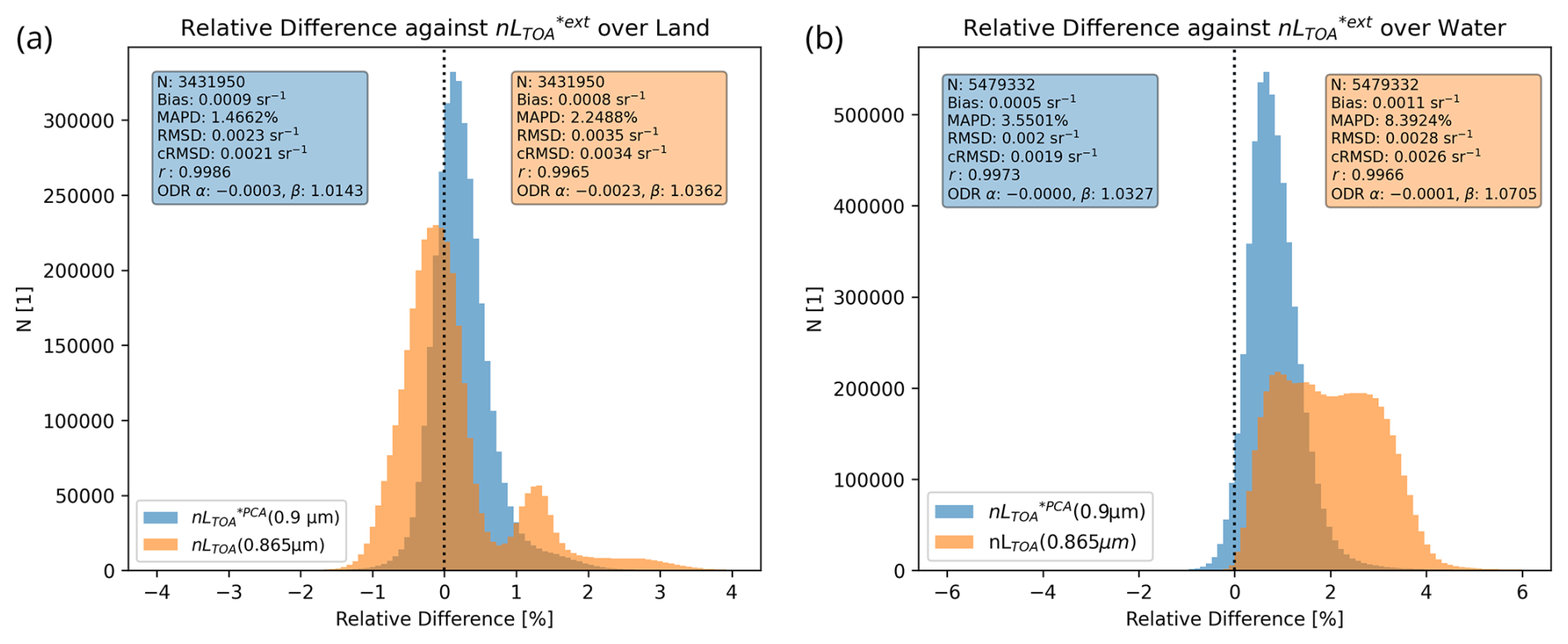
Figure 3 Relative differences between two proposed ${\mathrm{nL}}_{\mathrm{TOA}}^{*}$ against the extrapolated ${\mathrm{nL}}_{\mathrm{TOA}}^{*\mathrm{ext}}$ as used in the COWa algorithm over land (a) and water surfaces (b), respectively. ${\mathrm{nL}}_{\mathrm{TOA}}^{*\mathrm{PCR}}$ from the PCR in blue and the relative difference between extrapolated ${\mathrm{nL}}_{\mathrm{TOA}}^{*\mathrm{ext}}$ and nL_TOA(0.865 µm) in orange. The associated metrics in the corresponding colours are found in the top corners. The solid black line indicates 0 % relative deviation.

Using the OLCI/SLSTR synergy allows us to assess the performance of the PCR to estimate τ_pTOA rather than directly using the window (nL_TOA(0.865 µm)) against a common reference. In the Copernicus Sentinel-3 OLCI Water Vapour product (COWa) algorithm, ${\mathrm{nL}}_{\mathrm{TOA}}^{*}$(0.9 µm) is extrapolated from the two adjacent window bands at 0.865 and 0.885 µm (Preusker et al., 2021). For τ_pTOA(0.94 µm), ${\mathrm{nL}}_{\mathrm{TOA}}^{*}$(0.94 µm) is interpolated from the two window bands 0.885 and 1.020 µm. This is substantially closer to the “real” surface reflectance than using the PCR. Hence, we compare ${\mathrm{nL}}_{\mathrm{TOA}}^{*\mathrm{PCA}}$(0.9 µm) against ${\mathrm{nL}}_{\mathrm{TOA}}^{*\mathrm{ext}}$(0.9 µm) from the extrapolation using the two adjacent window channels. For this and other comparisons, we calculated the relative difference in per cent by dividing the absolute difference (observation minus reference) by the reference multiplied by the factor 100. Fig. 3a and b reveal that the vast majority of points lie close to the 0 % line for both land and water pixels, albeit with a positive bias. In contrast, using the 0.865 µm normalized radiance by itself would yield much worse results, i.e. a strong bi-modal distribution over land and a weaker bi-modal distribution with a wide spread over water (see Fig. 3a and b).

On average, there is a small positive bias in ${\mathrm{nL}}_{\mathrm{TOA}}^{*\mathrm{PCA}}$(0.9 µm), both over land (+0.3 %) and water (+0.8 %). Over land pixels, the 98th percentile of the relative percentage deviation is 1.7 % against the 2.6 % when using nL_TOA(0.865 µm) as ${\mathrm{nL}}_{\mathrm{TOA}}^{*}$. Over water pixels, the 98th percentile of the relative percentage deviation lies at 2.2 %, whereas this value is 4 % when using nL_TOA(0.865 µm) as ${\mathrm{nL}}_{\mathrm{TOA}}^{*}$. On average, an increase of 1 % in ${\mathrm{nL}}_{\mathrm{TOA}}^{*}$(0.9 µm) approximately translates to a 1.6 % increase (approx. 0.9 kg m⁻²) of TCWV estimate. A correction of this bias may be possible, but since such an analysis cannot be carried out using FCI, we decided against it. Because the PCR performed better than the window channel by itself, we decided to use ${\mathrm{nL}}_{\mathrm{TOA}}^{*\mathrm{PCA}}$(0.9 µm) to calculate τ_pTOA over both land and water surfaces. Despite the slight deviations, the PCR approach remains a good technique in order to reduce the impact of the spectral slope as much as possible.

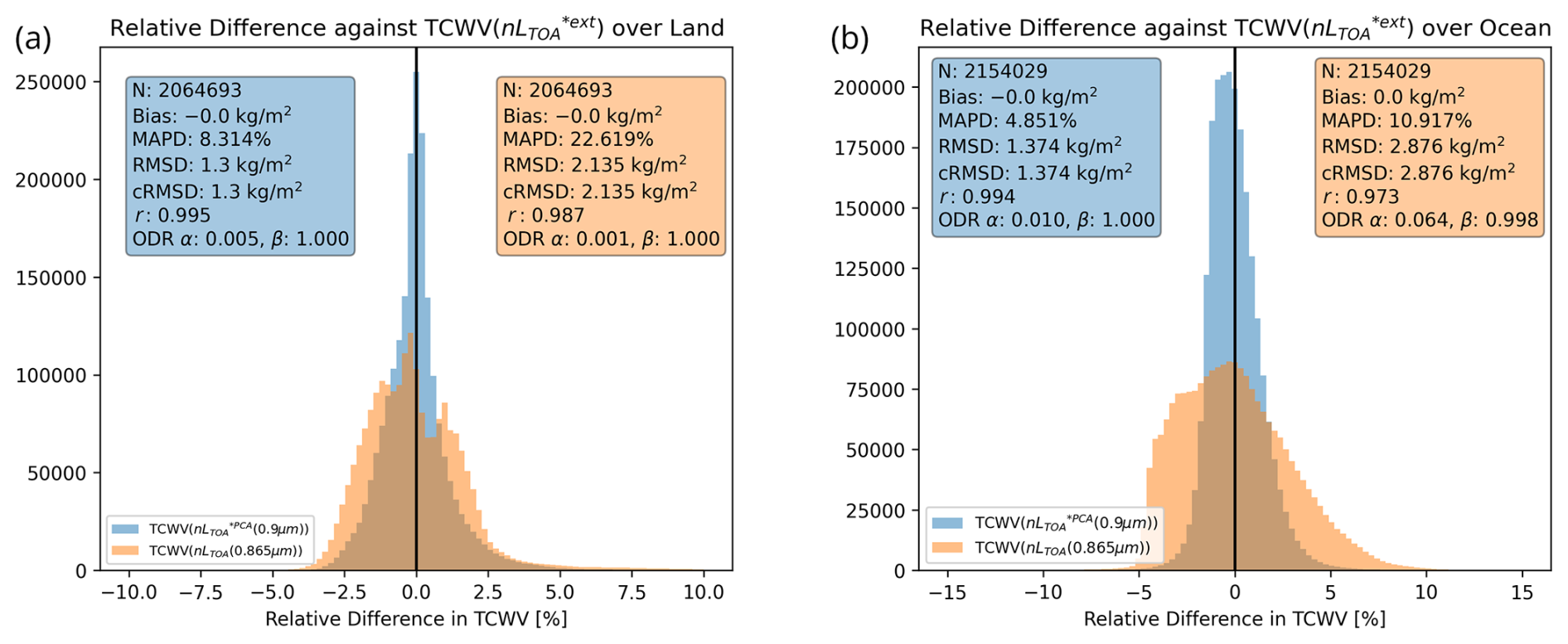
Figure 4 Relative difference between TCWV retrieved with τ_pTOA calculated from extrapolated ${\mathrm{nL}}_{\mathrm{TOA}}^{*\mathrm{ext}}$ and ${\mathrm{nL}}_{\mathrm{TOA}}^{*\mathrm{PCR}}$ from the PCR in blue and τ_pTOA calculated from nL_TOA(0.865 µm) in orange. Results are shown for land pixels (a) and for ocean pixels (b). The TCWV has been bias-corrected against the reference (TCWV using ${\mathrm{nL}}_{\mathrm{TOA}}^{*\mathrm{ext}}$). The data are for a random subset of one day in June 2021. The associated metrics in the corresponding colours are found in the top corners. The solid black line indicates 0 % relative deviation.

This can also be demonstrated using a TCWV processed from a single day of OLCI/SLSTR observations. Here, we compared the retrievals from using each ${\mathrm{nL}}_{\mathrm{TOA}}^{*\mathrm{ext}}$, ${\mathrm{nL}}_{\mathrm{TOA}}^{*\mathrm{PCA}}$, and nL_TOA(0.865 µm) to calculate τ_pTOA as input to the algorithm. In order to only see the influence on precision of TCWV, both datasets have been bias-corrected. The results are shown in Fig. 4. Over land surfaces, the bi-modal distribution in using nL_TOA(0.865 µm) persists with large spread and systematic over- and underestimations. Over the ocean, the difference between the two approaches is even more pronounced. Both MAPD and RMSD indicate that using ${\mathrm{nL}}_{\mathrm{TOA}}^{*\mathrm{PCR}}$ instead of nL_TOA(0.865 µm) for the calculation of τ_pTOA improves the retrieval substantially.

In very rare cases (< 0.1 %), there are large deviations (> 5 %). Upon visual inspection, these extreme deviations mostly occur along rivers, coasts, in high elevations, or at the poles. We explain these cases by (1) unidentified clouds, (2) coastal and inland water pixels with mixed contributions by land and water, (3) water-constituents changing the NIR reflectance of the water surface substantially, (4) adjacency effects, the brightening effect of dark pixels by diffuse radiation from neighbouring bright pixels, and (5) geolocation and unphysical spectral matches between OLCI and SLSTR. Yet, these rare deviations are still lower than the extreme deviations found by using the window band at 0.865 µm itself.

3.5 Finalized retrieval framework

The retrieval procedure is as follows. FCI (or OLCI/SLSTR) radiometric and ancillary data are read and the necessary auxiliary fields (ECMWF forecast, AOT) are interpolated to satellite resolution. In the next step, the cloud mask and the measurements (e.g. reflectances, τ_pTOA, etc.) are calculated. A land and water processing mask is produced. Pixels which are marked as cloudy or where SUNZ is too slant (> 80°) are filtered out.

The inversion is run up until the pre-defined convergence criterion is reached. Once this is reached, this state is passed out of the algorithm and these pixels are marked as converged. If the algorithm exceeds the maximum allowed number of iterations (six over land, eight over ocean), the inversion stops, and these pixels are marked as not-converged. Furthermore, the algorithm's output includes the associated retrieval error covariance of the final state.

After the processing has finished for all pixels, data are only marked as valid if their cost is below a threshold (currently < 1) and if the convergence criterion has been met. Such a check may filter out some cloudy pixels which have been missed by the cloud mask or pixels which contain a thick and/or elevated aerosol layer. Here, an extremely high cost may be caused by a substantial underestimation of TCWV with regard to the prior/first guess TCWV owing to the shielding effect. However, a higher cost does not necessarily relate to a failed retrieval.

4 Results

4.1 Sentinel3 OLCI and OLCI/SLSTR data

An initial test for our forward model and the inversion technique was the application to an existing matchup database used for the validation and quality control of COWa. OLCI measurements were spatio-temporally collocated with the ARM network site Southern Great Plains (SGP) positioned in the Midwest of the United States of America. The dataset is limited to one location only and runs from 2016 to 2023. Since SLSTR measurements are missing from this dataset, the approximation of ${\mathrm{nL}}_{\mathrm{TOA}}^{*\mathrm{PCR}}$ in the absorption band using the PCA regression could not be done. Instead, we chose the same approach as COWa: extrapolate nL_TOA from band 17 (0.865 µm) and band 18 (0.885 µm) to band 19 (0.9 µ m).

The analysis of the two-band OLCI TCWV is shown in Fig. 5 and yields a strong correlation with a Pearson correlation coefficient (r) of 0.995. The bias of 1.848 kg m⁻², orthogonal distance regression (ODR) coefficients, i.e. offset (α) and slope (β) of 1.122 and 1.038, respectively, indicate a slight wet bias. The cRMSD of 1.256 kg m⁻², RMSD of 2.235 kg m⁻² and MAPD of 13.433 % still indicate slight spread.

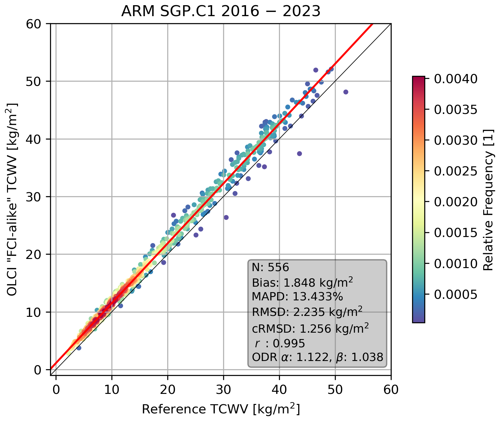
Figure 5 Comparison of S3OLCI “FCI-like” TCWV (using ${\mathrm{nL}}_{\mathrm{TOA}}^{*\mathrm{ext}}$) against ARM TCWV at the SGP site, coloured with the relative frequency of occurrence. The solid black line presents the 1 : 1 line, the red line marks the ODR curve.

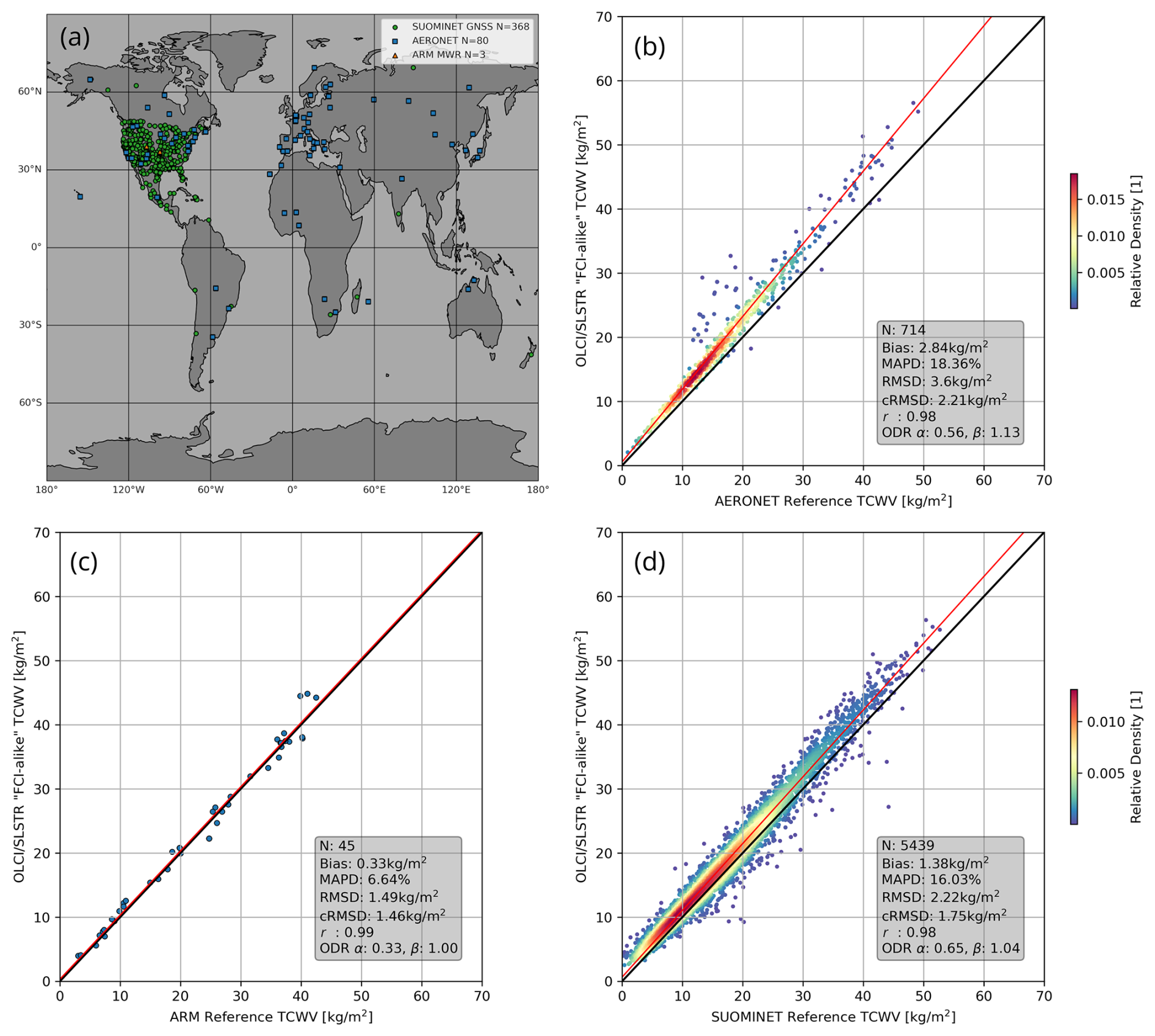
Figure 6 Matchup Analysis of OLCI/SLSTR “FCI-like” TCWV against globally distributed reference sites. The geographical distribution and their sum of all reference sites from which reference TCWV datasets are used in the matchup analysis are shown in panel (a). The analysis results against AERONET is shown in panel (b), against ARM is shown in panel (c) and against SUOMINET is shown in panel (d). This TCWV uses the PCR approach to estimate τ_pTOA. The solid black lines present the 1 : 1 line, and the red lines mark the respective ODR curves.

In the next step, we processed the global dataset of the OLCI/SLSTR synergy. This was done to assess the quality of the two-band approach and the LUT-inversion in combination with the PCR approach to estimate τ_pTOA (0.9 µm). This TCWV was compared against three different reference networks. For this matchup analysis, we followed the same matchup procedure as before. The results of the comparisons are depicted in Fig. 6b to d. Figure 6a shows the positions of the ground-based reference sites with at least one valid matchup according to their network. For the ARM network, only three stations in North America were available for 2021. With AERONET and SUOMINET, a wider range of different climate zones and atmospheric conditions can be covered. The comparison of 714 valid matchups against 80 AERONET stations in Fig. 6a reveals a wet bias of 2.84 kg m⁻², a MAPD of 18.36 %, a RMSD of 3.6 kg m⁻², cRMSD of 2.21 kg m⁻², r of 0.98, and ODR offset and slope of 0.56 and 1.13, respectively. The analysis results for 45 valid matchups against ARM MWR observations can be seen in Fig. 6b and show a slight wet bias of 0.33 kg m⁻², a MAPD of 6.64 %, a RMSD of 1.49 kg m⁻², a cRMSD of 1.46 kg m⁻², r of 0.99, and ODR offset and slope of 0.33 and 1, respectively. In the comparison of 5439 matchups against 368 SUOMINET stations shown in Fig. 6d, we find a wet bias of 1.38 kg m⁻², a MAPD of 16.03 %, RMSD of 2.22 kg m⁻², a cRMSD of 1.75 kg m⁻², a r of 0.98, and ODR offset and slope of 0.65 and 1.04, respectively. Most SUOMINET stations are positioned in Central and North America.

4.2 MTG-FCI data

To test our algorithm with regard to future nominal FCI data, we applied the first prototype on test data provided by EUMETSAT. Since this dataset is still preliminary, this is neither a definitive nor quantitative assessment. Rather, it serves to check the processor's performance with real data and check the product for any unexpected behaviour and/or defects. The data were gathered on 13 January 2024 at 11:50 UTC. The full disc true colour RGB and processed TCWV are depicted in Fig. 7a and b, respectively.

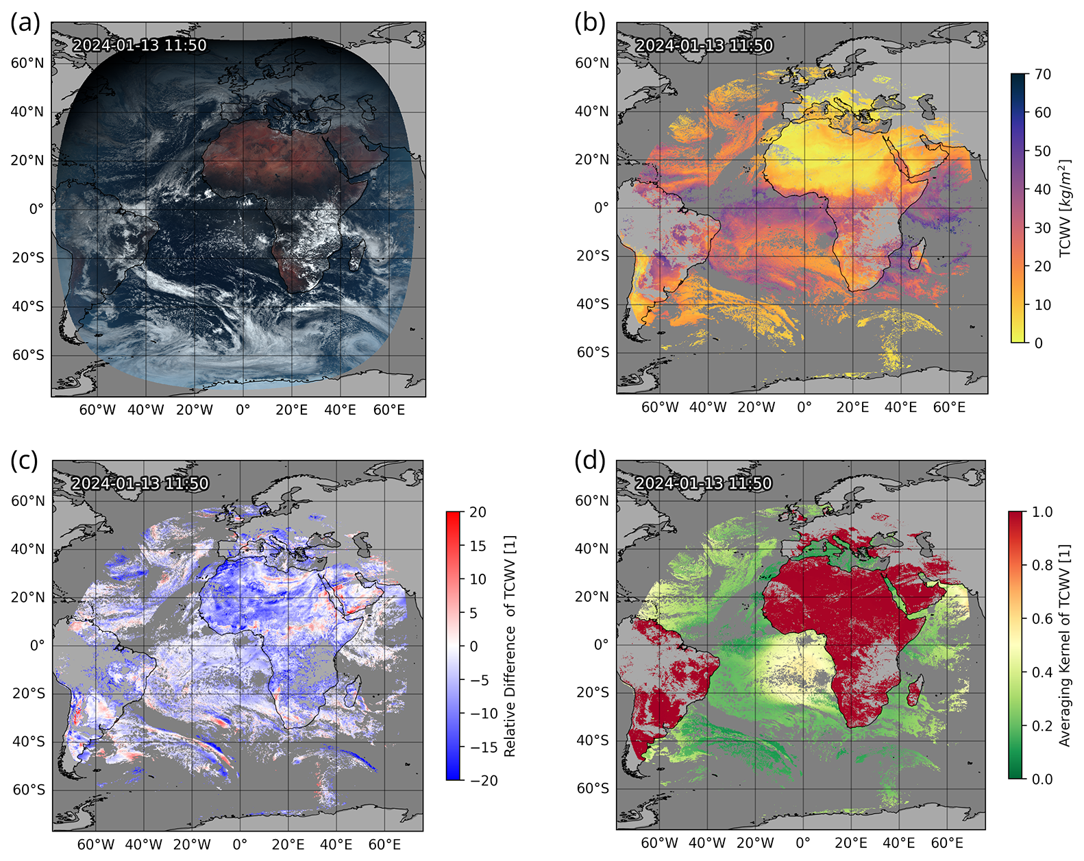
Figure 7 Full disc visualization of a true colour composite in panel (a), TCWV in panel (b), the relative difference between FCI TCWV and ERA5 reanalysis TCWV in panel (c) and AVK corresponding to the retrieved TCWV in panel (d). and related products, processed from FCI data acquired on 13 January 2024. Dark grey marks land surfaces, light grey marks water surfaces.

In parallel processing, the running time of one full disc scene on a workstation with 64 GB of RAM and a 12 core CPU is less than 5 min. In single processing, the running time of a single chunk takes approximately 30 to 50 s. This includes input/output operations, cloud-masking, PCR, and inversion.

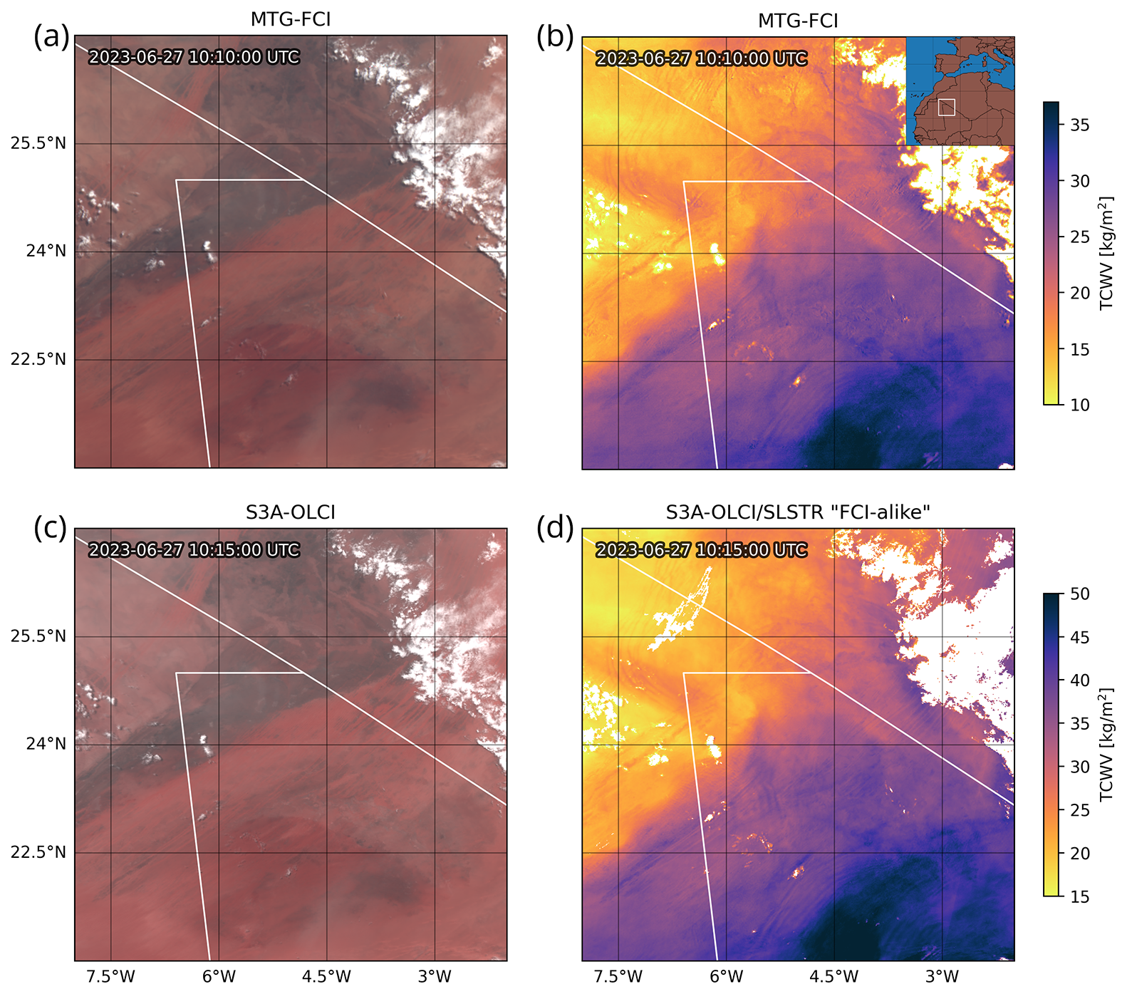
Figure 8 Comparison of FCI TCWV and OLCI/SLSTR “FCI-like” TCWV for a close-up on 27 June 2023 over Northern Mali. The FCI true colour composite is shown in panel (a), the FCI TCWV is shown in panel (b). The coinciding OLCI true colour composite is shown in panel (c), the OLCI “FCI-like” TCWV is shown in panel (d).

In Fig. 7b, arid regions such as the Sahara or the Arabian Peninsula are clearly visible. Europe also exhibits low TCWV. Synoptic features such as bands of elevated moisture are visible. Despite the wide range of viewing zenith and solar zenith angles and their implications for the line of sight, there appears to be no influence on the TCWV product. Over Central Africa, some clouds that are visible in the RGB have not been detected by the cloud mask. Such areas are also distinguishable by their decreased TCWV values compared to the surrounding areas. This underestimation owing to clouds as well as the finer details can be seen in a close-up of the scene in Fig. 8b. Because of the 1 km resolution of FCI's NIR channels, we can also detect meso- to mini-scale features such as smaller pockets of high moisture over the ITCZ or the mixing between dry and moist air masses. Closer to the shore, the TCWV field shows slight discontinuities between the water and land surface. The water-pixels close to the shoreline often show values which deviate a few per cent from the adjacent land-pixels; in most cases, there is an overestimation.

At this stage, a rigorous quantitative validation of the TCWV product is not feasible, and our comparison against TCWV from the ERA5 reanalysis is not intended as such. As a preliminary way to check the TCWV field for consistency, we plotted the relative difference between the FCI TCWV and a collocated ECMWF ERA5 reanalysis TCWV, shown in Fig. 7c. This gives us a first impression whether any artefacts or defects appear or whether the algorithm works as intended. The image in Fig. 7c is dominated by negative differences, which translates to a dry bias against the reanalysis TCWV. On average, FCI TCWV is approximately 10 % drier than the reanalysis over land surfaces and 5 % drier over water surfaces. Furthermore, there are areas with positive and negative differences close to one another, often resembling a line, e.g. over Northern Africa or over the South Atlantic. Figure 7d depicts the AVK at each pixel. Over land, the value is close to 1 for most pixels since the forward model is very sensitive to changes in the measurements. Over water, this value lies between 0 and 0.7. In areas of sunglint, the AVK ranges from 0.4 to 0.7. In areas with low water-surface reflectance, the AVK approaches 0. Areas with increased AMF and/or TCWV exhibit a slightly higher AVK between 0.1 and 0.3.

To showcase FCI's spatial resolution, we compare a TCWV field from Sentinel3-A OLCI/SLSTR with real preliminary calibrated FCI from 27 June 2023 in Fig. 8. Both are processed with the algorithm described above. The temporal difference between the two fields is approximately 5 min. The scene is situated in northern Mali in West Africa. The differences in viewing geometry are visible between FCI and OLCI. In the true colour RGB of FCI, longer cloud shadows are visible, which are much smaller in the S3A-OLCI image, or their positions are shifted. The TCWV fields reveal a moist air mass in the south east, while a drier air mass is positioned in the north west. Consistent with the comparison against the ERA5 analysis, FCI TCWV is approximately 10 % lower than OLCI TCWV. Hence, another colour map range is used in the FCI TCWV image (Fig. 8b).

FCI is capable of reproducing the amount of detail found in the OLCI TCWV field: e.g. a dry line in the western half of the image (i.e. strong gradients in moisture between the air masses) or gravity waves in the southern half or north-eastern corner (local, wave-like peaks and troughs in TCWV). The positioning of features appears to be coherent between the two sensors. Furthermore, we can see slight indications of FCI's scan-lines in Fig. 8b. These are noisy pixels that follow lines that run from east to west. The effect is more pronounced over water surfaces. In both figures, the effect of unidentified cloud pixels on the TCWV is visible as decreased TCWV at cloud edges. In contrast, there are some thin dust layers visible in the north-western and central-eastern parts of the RGBs, which do not show in either of the TCWV products.

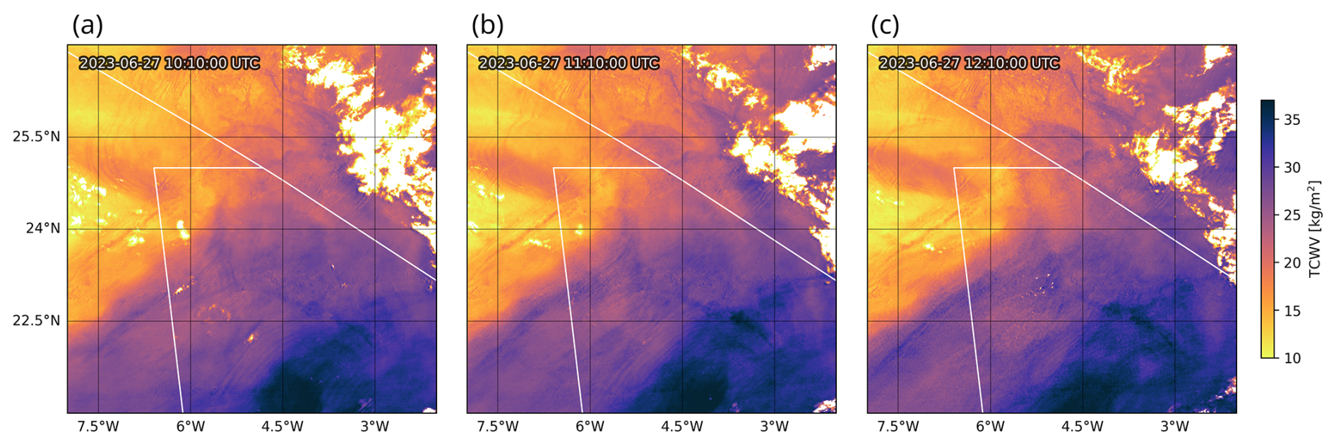
Figure 9 Time sequence of FCI TCWV shown in Fig. 8b with 1 h between each frame.

To further highlight the potential of FCI TCWV observations for convective nowcasting purposes, we showcase the TCWV field from Fig. 8b again in Fig. 9 with the TCWV from two time steps later in Fig. 9a to c. The sequence demonstrates how one can track the propagation of the gravity waves and the north-western movement of the moist air mass along the moisture-front. The formation of what appear to be small updrafts or thermals is indicated by stark increases in TCWV from Fig. 9b to c. This results in a pattern similar to convective rolls shown in Carbajal Henken et al. (2015). In the lower centre, first clouds are forming at around 11:40 UTC.

5 Discussion and outlook

In the multiannual validation against the reference ARM SGP TCWV dataset (2016–2023), the OLCI 2-band TCWV shows a good performance with a bias of 1.848 kg m⁻², RMSD of 2.235 kg m⁻², cRMSD of 1.256 kg m⁻², and high r of 0.99. The wet bias may be corrected following the procedure described in Preusker et al. (2021). In a comparison against their COWa algorithm applied to the same matchup dataset, they have a similar r of 0.99 but a lower RMSD of 1.3 kg m⁻², which may well be attributed to both the use of an additional absorption band at 940 nm and initial τ_pTOA-correction. Such a good performance against the reference TCWV is promising. However, for this comparison, τ_pTOA has been estimated from two adjacent window bands (i.e. the same way COWa estimates τ_pTOA).

For FCI, the accuracy of τ_pTOA and subsequently TCWV mostly hinges on the PCR's ability to estimate the spectral slope. As shown in Fig. 3, the approximation shows a good performance against the next-best estimate, i.e. extrapolation from two adjacent window bands using OLCI measurements, and exceeds the performance of just using the window band at 0.865 µm. Approximated ${\mathrm{nL}}_{\mathrm{TOA}}^{*}$ may deviate from the reference ${\mathrm{nL}}_{\mathrm{TOA}}^{*}$ on average by 1.5 % over land and 3.5 % over water. In rare cases, the PCR failed. We assume that there may be several processes at play that require deeper investigations. Mis-characterizations of the surface reflectance translate to an additional uncertainty of about 1 to 2 kg m⁻². Nevertheless, these initial results demonstrate that our approach is effective and advancing well towards an operational TCWV retrieval framework for FCI.

The global comparison against the reference networks returned slightly lower performance indicators with r between 0.98 and 0.99, bias between 0.33 and 2.84 kg m⁻², MAPD between 6.64 % and 18.36 %, RMSD between 1.49 and 3.6 kg m⁻², and cRMSD between 1.46 and 2.21 kg m⁻². The highest RMSD and bias are found in the comparison against AERONET, which is probably due to AERONET's dry bias (Pérez-Ramírez et al., 2014). The OLCI/SLSTR matchup analysis shows a decreased performance against the multi-year matchup of only OLCI over ARM SGP. This is due to a reduced number of matchups over a shorter time span and a higher geographic spread. A more rigorous validation would require a longer time period. However, the aim of this assessment is to show that the PCR does not drastically reduce the algorithm's performance. The actual performance of FCI TCWV may deviate from these verification results since the spectral characteristics and calibration are different from OLCI. Future validation studies have to be conducted for further characterization, which may also lead to a more elaborate correction for initial τ_pTOA estimation.

To assess the functionality of the current algorithm prototype, we applied it to the FCI Level 1c test dataset provided by EUMETSAT. Conceptually, everything is in working order. The running times are close to or below the 5 min mark (FCI's nominal temporal resolution on a 2024 computer) and allow for a near-real-time and operational application of our TCWV algorithm. Full disc comparisons show that the algorithm produces a sensible TCWV field. The relative difference between collocated ECMWF ERA5 reanalysis TCWV at 12:00 UTC and FCI TCWV product reveals a systematic dry bias of approximately 8 %. We suspect three probable reasons for this systematic dry bias: (1) the bias might be related to the preliminary calibration of the FCI data, (2) the PCR systematically overestimates the surface reflectance at 0.914 µm and thus τ is too low and (3) undetected deficits in our LUTs. If this systematic bias persists and no underlying reason can be found, we may mitigate it using the empirical correction method described in Preusker et al. (2021). Furthermore, there are large-scale patterns of positive and negative deviations close to one another. Such patterns are to be expected in a comparison against model data and indicate that the model struggles with accurately capturing the advection of air masses in both space and time. The observed TCWV fields might be closer to the actual state.

FCI's TCWV AVK of almost 1 indicates a high sensitivity to the measurement and only a small contribution of prior knowledge. This can be interpreted as the algorithm being independent of the NWP input. This is a key advantage of NIR TCWV in contrast to other satellite-retrieved TCWV. The decreased TCWV AVK over water surfaces is caused by the much lower water surface reflectance in the NIR. In cases in which the reflectance is close to 0, the retrieval is challenging. However, the OE may still provide an update of the a priori TCWV field. Over sunglint, the AVKs above 0.4 indicate that the retrieval is much more independent of the a priori and much more reliable.

Comparing OLCI and FCI TCWV up close, we can easily see that FCI TCWV matches the level of detail found in the OLCI TCWV product. For scenes over Europe, FCI's resolution will be slightly lower compared to OLCI's reduced resolution. Yet, FCI's resolution will be significantly higher than SEVIRI's. The stripes of enhanced noise that run across the FCI TCWV image are caused by scan-lines of FCI. Similar scan-line artefacts are found in whisk-broom sensors such as MODIS or the Visible Infrared Imaging Radiometer Suite (VIIRS), too. Over land this is barely noticeable. However, over dark water pixels it is pronounced. This may change in future Level 1c processing versions. The assessment exercises discussed above helped us identify several limitations and challenges regarding TCWV retrievals from FCI measurements. The presence of clouds is visible as pixels with considerably lower TCWV than their surrounding. A robust cloud mask is needed to filter out such pixels. At a later stage, such retrieved pixels may be used for an “above cloud” WV product. Such a product may then be used for the detection of WV entrainment into the stratosphere, e.g. in the presence of overshooting tops (Setvák et al., 2008; Dauhut et al., 2018; Khordakova et al., 2022).

While the PCR yields reliable ${\mathrm{nL}}_{\mathrm{TOA}}^{*}$ over the vast majority of surface types, in some cases it deviates far from the reference. This may be addressed by extending the training dataset the PCs are calculated from.

So far, we use a fixed aerosol type, height, and thickness. Under conditions violating these assumptions (e.g. a strong dust outbreak), retrieval quality would be decreased. We are considering simulating for additional aerosol mixtures and aerosol layer heights. Furthermore, using AOT forecasts from the Copernicus Atmosphere Monitoring Service (CAMS) could improve the retrieval. Another issue is that over water surfaces, the inversion framework is under-determined: a measurement vector with only two elements (nL_TOA(0.865 µm), τ_pTOA (0.914 µm)) is opposed by a state vector with three elements (TCWV, AOT, WSP). Outside sunglint, the influence of the wind speed is marginal, and AOT mainly increases the TOA signal (and thus the forward model is not sensitive to changes of the wind speed), and inside sunglint the influence of a thin layer of aerosol is reduced. Because of that, the information content is relatively balanced, and the impact is slightly reduced. Nevertheless, over water surfaces, adding a third channel to the measurement vector (e.g. 0.51 or 1.61 µm) may also improve the performance.

With FCI, we are able to monitor the temporal evolution of these small-scale patterns at a resolution similar to OLCI's. This allows for the tracking of large- and small-scale dynamics before, during, and after convective development. Such features and their changes (e.g. convergence zones, convective rolls, deepening boundary layers) contain potential information for nowcasting purposes. Furthermore, the patterns observed in FCI TCWV may also be tracked and used to retrieve lower level atmospheric motion vectors.

Our framework may be adapted to provide accurate TCWV retrievals for other sensors featuring at least two channels in and around the ρστ band. The National Oceanic and Atmospheric Administration (NOAA) is commissioning GeoXO Imager (GXI), the successor to the Advanced Baseline Imager (ABI) on the Geostationary Operational Environmental Satellite – 3rd generation (GOES), which will include a WV absorption band in the ρστ region (Lindsey et al., 2024). Another future instrument soon to be launched into a polar orbit is METImage, flying onboard EUMETSAT's Meteorological Operational satellite second generation A (METOP-SG-A) (Phillips et al., 2016). METImage will enable NIR TCWV with a spatial resolution of 500 m and global coverage every day. METImage will also provide O2A band measurements (around 0.76 µm), which can be used to reduce ambiguity owing to shielding of cirrus or elevated aerosol layers. A NIR TCWV product from METImage may then be used in advanced synergies with sounders such as Infrared Atmospheric Sounder Interferometer – New Generation (IASI-NG), which will also be flying on METOP-SG-A. IASI-NG is the successor of IASI, which provides all-sky temperature and humidity profiles with a slightly lower accuracy in the presence of clouds (Müller, 2017).

Furthermore, the Infrared Sounder (IRS) will be operating on MTG-S1, MTG-I1's sister satellite, and will cover the same field of view as FCI. This will enable a synergy between TCWV from FCI and the IRS humidity profile product. NIR TCWV could very well complement profile soundings for both IASI-NG and IRS: one shortcoming of these retrievals is their low or missing sensitivity to the lowest layers of the troposphere (below 1–2 km). Furthermore, their spatial resolution is in the order of tens of km, often insufficient for assessing small-scale weather patterns. A high-spatial resolution NIR TCWV product, sensitive to the whole column of air, could complement such sounding products perfectly, albeit in the absence of clouds. A synergy could consist in an updated layer product or a product that provides the moisture content of the lowest levels of the troposphere. Such synergy products could provide crucial insights into meteorological conditions, such as the atmospheric instability, and improve the potential for the prediction of severe weather.

6 Conclusions

Leveraging our expertise in TCWV retrievals from NIR measurements for various satellite-based passive imagers, we developed a new retrieval framework for the new Meteosat Third Generation Flexible Combined Imager (MTG-FCI) measurements. The use of OLCI/SLSTR synergy “FCI-like” data proved valuable for establishing and validating an adapted TCWV retrieval framework for MTG-FCI. It offers a realistic and reliable test bed that supports algorithm development ahead of the availability of a sufficiently long and calibrated FCI data record. Key challenges, such as the surface reflectance treatment in the WV absorption band, can be addressed in preparation for the large-scale application of the retrieval to FCI data.

The evaluation exercises highlight the robustness of the retrieval framework and have helped in identifying specific challenges and limitations related to the MTG-FCI instrument, which can be further addressed with fully calibrated FCI data in the near future.

As the successor to MSG-SEVIRI, MTG-FCI boasts extended observational and spectral capabilities that promise significant advancements in weather and climate research and applications, particularly in the monitoring and study of atmospheric TCWV amounts and dynamics. Notably, FCI is the first geostationary satellite instrument with measurements in the NIR ρστ WV absorption band. While SEVIRI TIR measurements allowed to derive information on WV amounts mainly in higher parts of the troposphere, the FCI NIR WV absorption measurements exhibit the greatest sensitivity to WV amounts near the surface. This enables accurate and high temporal resolution observations of changes in moisture content in the lower troposphere. Consequently, these novel and comprehensive TCWV observations will enhance the (real-time) monitoring of atmospheric moisture distributions in the boundary layer, their evolution, and associated meteorological phenomena across regional to continental scales, with the potential to significantly advance nowcasting techniques.

Appendix A: List of variables and their respective explanations

Variable	Definition/explanation
A	averaging kernel matrix
a	τpTOA correction offset
b	τpTOA correction slope
ALB	surface albedo, i.e. surface irradiance reflectance
AMF	air mass factor
AVK	averaging kernel
cwin	regression coefficient vector
ϵ	forward model uncertainty
ϵintp	${\mathrm{nL}}_{\mathrm{TOA}}^{*}$ approximation uncertainty
F	forward model
F0	spectral solar irradiance
G	gain matrix
K	jacobian matrix
λ	wavelength
LTOA	top-of-atmosphere radiance
nLTOA	normalized top-of-atmosphere radiance
${\mathrm{nL}}_{\mathrm{TOA}}^{*}$	normalized top-of-atmosphere radiance corrected for WV attenuation
${\mathrm{nL}}_{\mathrm{TOA}}^{*\mathrm{ext}}$	${\mathrm{nL}}_{\mathrm{TOA}}^{*}$ estimated from extrapolation of window bands
${\mathrm{nL}}_{\mathrm{TOA}}^{*\mathrm{PCA}}$	${\mathrm{nL}}_{\mathrm{TOA}}^{*}$ estimated from principle component regression
p	parameter vector
r	Pearson correlation coefficient
S	spectral slope
Rtarget	reflectance vector of target
Rwin	reflectance vector of window channels (source)
ρ	irradiance ratio reflectance
ρTOA	irradiance ratio reflectance at top-of-atmosphere
$\widehat{\mathbf{S}}$	retrieval error covariance matrix
Sa	a priori state error covariance matrix
Sϵ	measurement error covariances matrix
SATA	satellite azimuth angle
SATZ	satellite zenith angle
SNR	signal-to-noise ratio
SUNA	sun azimuth angle
SUNZ	sun zenith angle
τpTOA	pseudo optical thickness
Utarget	principle components folded to target band spectral response functions
Uwin	principle components folded to window band spectral response functions
RAZI	relative azimuth angle
RAZI	relative azimuth angle
x	state vector
$\widehat{\mathit{x}}$	true state vector
xa	a priori state vector
y	measurement vector