δ¹³C carbon isotopic composition of CO₂ in the atmosphere by Lidar – a preliminary study with a CDIAL system at 2 µm

Our understanding of the global carbon cycle needs for new observations of CO₂ concentration at different space and time scales but also would benefit from observations of additional tracers of intra-atmospheric or surface-atmosphere exchanges to characterize sources and sinks. Lidar is a well-known promising technology for this research as it can provide, at the same time, structure of the atmosphere, dynamics and composition of several trace gas concentration. In this framework, a coherent differential absorption lidar (CDIAL) has been developed at LMD to measure simultaneously and separately ¹²CO₂ and ¹³CO₂ isotopic composition of CO₂ in the atmosphere. It also provides the radial wind speed along the line of sight of the laser. This paper investigates the methodology of three wavelengths DIAL in the spectral domain of 2 µm to obtain range-resolved CO₂ isotopic ratio δ¹³C. The set-up of the lidar as well as the signal processing is described in details. First atmospheric measurements along three days are achieved in the surface layer above the suburban area of Ecole Polytechnique campus, Palaiseau, France. Typical performances of the instrument (median values along 70 h of measurement) with 10 min of time averaging show: (1) a precision around 0.6 % for 1.2 km range resolution for ¹²CO₂ mixing ratio (2) a precision around 3.2 % for 1.6 km range resolution for ¹³CO₂ mixing ratio. In situ co-located gas analyser measurements are used to correct for biases that are explained neither by the spectroscopic database accuracy nor the signal processing and will need further investigation. Nevertheless, this preliminary study enables to make a useful state of the art for current lidar ability to provide δ¹³C measurements in the atmosphere with respect to geophysical expected anomalies and to predict the necessary performances of a future optimized instrument.

1 Introduction

CO₂ is the main anthropogenic greenhouse gas responsible for the current global warming. In 2024, its global annual average concentration in the atmosphere has reached more than 420 ppm and the global mean near surface temperature is 1.5 °C above the 1850–1900 average, with significant consequences for present and future life on planet Earth (WMO, 2025; IPCC, 2023). In our understanding of the carbon cycle, it is fundamental to associate a number of CO₂ molecules with their original surface or atmospheric sources and sinks. In particular, the biospheric sink remains very complex to assess at regional scale with current tools (bottom-up or top-down methods) given the strong ecosystem space and time heterogeneity (Friedlingstein et al., 2020). The mitigation of anthropogenic emissions needs as well other clues than a standard CO₂ mixing ratio measurement to assign a number of molecules to the type of emission: coal, gas, fuel, natural vs anthropogenic.

In this context, the CO₂ stable isotopic fraction δ¹³C is an interesting tracer for CO₂ surface-atmosphere exchanges at local scale. It enables to characterize plant/soil physiological processes (photosynthesis, respiration, decomposition of organic matter) and may help to issue a diagnosis on sources (anthropogenic, geological) and sinks (biosphere, ocean) of CO₂. In addition, δ¹³C can discriminate the type of plant (C₃ or C₄) and ecosystems that contribute the most to biosphere CO₂ uptake and their evolution with warming conditions (Buchmann n and Ehleringer, 1998; Flanagan et al., 1996). While the difference between C₃- and C₄-dominated biomes provides the largest observed variation in δ¹³C (Still et al., 2003), even within pure C₃ ecosystems, a large temporal and spatial variability of δ¹³C is observed during nighttime respiration process due to species-specific effects and environmental conditions such as light, temperature and water availability, the latter being a major driver (Buchmann et al., 1997; Brugnoli et al., 1998; Bowling et al., 2002; Ekblad and Högberg, 2001; Pataki et al., 2003; Mortazavi et al., 2005). The natural variation of δ¹³C source spreads over a scale of 100 ‰: ∼ +5 ‰ for carbonate-gas CO₂ equilibrium in air-sea/geological water exchanges, −8 ‰ for standard CO₂ in the atmosphere, ∼ −14 ‰ for C₄ plant – air exchanges but ∼ −27 ‰ for C₃ plant that is similar to fossil fuel emission (coal and oil) whereas the lowest δ¹³C value, ∼ −40 ‰, can be found in natural gas emission (IAEA, 2008). However, hundreds of meters from the source, these anomalies are reduced to sub 1 ‰ variations due to efficient mixing of the atmosphere (Widory and Javoy, 2003).

Concerning current instrumentation and measurement, tunable diode laser absorption (Cassidy and Reid, 1982) or recent cavity ring down spectroscopy (Lin et al., 2020) offer a simpler way to make in situ measurements in the atmosphere compared to former complex mass spectrometry systems (Li et al., 2018). To increase the spatial scale representativity of in situ measurement, an integrated path differential absorption (IPDA) lidar concept at 4.4 µm has also been studied (Shi et al., 2022). Although such system seems to reach similar precision on δ¹³C (< 0.2 ‰) than in situ sensor, the horizontal profiling and 2-D mapping of the δ¹³C field above the surface by Lidar will bring new information on the patterns and origins of sources and sinks. Moreover, the vertical profiling will help characterize the local and long-distance transport of CO₂, in a similar way than Lidar measurements of water vapor stable isotopologues do already (Hamperl et al., 2022). However, 1 ‰ precision with hundreds of meters range resolution has not yet been reached for CO₂ DIAL system. Ultimately, the capability of ¹³CO₂ lidar measurements opens the way to a global monitoring of ¹³CO₂ from space using the IPDA technique to improve future global carbon inversion systems (Chen et al., 2017).

Several lidar teams have been interested in measuring CO₂ absorption with DIAL systems since almost 20 years with precursor work using DIAL systems in the 2 µm spectral band and coherent detection (Koch et al., 2004; Gibert et al., 2006) and more recent works (Gibert et al., 2015) reaching a precision of 0.5 % with 150 m and 15 min range and time resolution, respectively, close to what is needed for δ¹³C observations. The spectral band of 1.6 µm has also been considered with coherent DIAL (Yu et al., 2024) or direct detection DIAL, using the advantage of low noise internally amplified photodetector (Shibata et al., 2017; Yue et al., 2022; Stroud et al., 2023) although the obtained precision was limited by the ten times lower CO₂ absorption optical depth at such wavelength.

In this framework, a new three wavelengths coherent differential absorption Lidar (CDIAL) at 2 µm has been considered and recently developed at LMD to measure simultaneously ¹²CO₂ and ¹³CO₂ absorptions (Gibert et al., 2024). The purpose of this paper is to assess the current performances of the CDIAL system. The first sections describe the methodology and the spectral domain that has been chosen for this study. Then, a following section presents the experimental set-up, especially the new hybrid fibered/bulk laser source that was developed for this application. The signal processing is described in details to get the first lidar measurements of ¹²CO₂ and ¹³CO₂ mixing ratio. Current statistical and systematic errors are estimated. A discussion follows where the current performances of δ¹³C are compared to useful geophysical signals to be measured in the atmosphere. Some guidelines for δ¹³C efficient lidar measurements are pointed out.

2 Methodology

2.1 Multiwavelength DIAL theory

To measure the carbon isotopic ratio with the DIAL technique, at least three wavelengths have to be used, one serving as a reference, ideally located in a free-absorption spectral window. The differential absorption coefficients, α_i,exp, measured at the different wavelengths, are estimated with the mean range gate lidar backscattered signal power, P_i, as follows:

$$\begin{array}{}\text{(1)}& {\mathit{\alpha }}_{i,\exp }={\displaystyle \frac{\mathrm{d}{\mathit{\tau }}_{i,\exp }}{\mathrm{d}R}}={\displaystyle \frac{\mathrm{d}}{\mathrm{d}R}}\left[-{\displaystyle \frac{\mathrm{1}}{\mathrm{2}}}\ln \left({\displaystyle \frac{P_i}{P_{\mathrm{0}}}}\right)\right],\end{array}$$

where i = 1, 2 stands for ¹²CO₂ and ¹³CO₂ wavelengths respectively and i = 0 for the reference non-absorbed laser wavelength. τ_i,exp is the measured single path differential absorption optical depth (DAOD). Note that time and space averaging act at different scales in Eq. (1) that will be described later in the dedicated section on signal processing with biases and statistical error analysis. At this point, we just assume: (i) the laser wavelengths are closed enough that aerosol extinction and backscatter variations with wavelength are negligible and (2) the absorption variation is negligible in the range gate used to measure P_i.

The differential absorption coefficients are linked to the trace gas mixing ratios with:

$$\begin{array}{}\text{(2)}& \begin{array}{rl}& \left(\begin{array}{c}{\mathit{\alpha }}_{\mathrm{1},\exp }\\ {\mathit{\alpha }}_{\mathrm{2},\exp }\end{array}\right)\\ & ={\displaystyle \frac{n_{\mathrm{air}}}{\left(\mathrm{1}+C_{{\mathrm{H}}_{\mathrm{2}}\mathrm{O}}\right)}}\left(\begin{array}{ccc}\mathrm{\Delta }{\stackrel{\mathrm{̃}}{\mathit{\sigma }}}_{\mathrm{12}\mathrm{C},\mathrm{1}}& \mathrm{\Delta }{\stackrel{\mathrm{̃}}{\mathit{\sigma }}}_{\mathrm{13}\mathrm{C},\mathrm{1}}& \mathrm{\Delta }{\stackrel{\mathrm{̃}}{\mathit{\sigma }}}_{{\mathrm{H}}_{\mathrm{2}}\mathrm{O},\mathrm{1}}\\ \mathrm{\Delta }{\stackrel{\mathrm{̃}}{\mathit{\sigma }}}_{\mathrm{12}\mathrm{C},\mathrm{2}}& \mathrm{\Delta }{\stackrel{\mathrm{̃}}{\mathit{\sigma }}}_{\mathrm{13}\mathrm{C},\mathrm{2}}& \mathrm{\Delta }{\stackrel{\mathrm{̃}}{\mathit{\sigma }}}_{{\mathrm{H}}_{\mathrm{2}}\mathrm{O},\mathrm{2}}\end{array}\right)\left(\begin{array}{c}{C}_{\mathrm{12}}\\ C_{\mathrm{13}}\\ C_{{\mathrm{H}}_{\mathrm{2}}\mathrm{O}}\end{array}\right),\end{array}\end{array}$$

where $\mathrm{\Delta }{\stackrel{\mathrm{̃}}{\mathit{\sigma }}}_{\mathrm{12}\mathrm{C},i}$ = ${\stackrel{\mathrm{̃}}{\mathit{\sigma }}}_{\mathrm{12}\mathrm{C},i}-{\stackrel{\mathrm{̃}}{\mathit{\sigma }}}_{\mathrm{12}\mathrm{C},\mathrm{0}}$ and $\mathrm{\Delta }{\stackrel{\mathrm{̃}}{\mathit{\sigma }}}_{\mathrm{13}\mathrm{C},i}$ = ${\stackrel{\mathrm{̃}}{\mathit{\sigma }}}_{\mathrm{13}\mathrm{C},i}-{\stackrel{\mathrm{̃}}{\mathit{\sigma }}}_{\mathrm{13}\mathrm{C},\mathrm{0}}$ are the differential absorption cross-section (ACS), n_air = $p/\left(k_{\mathrm{B}}T\right)$ is the air density with T and p air temperature and pressure and k_B the Boltzman constant, $C_{{\mathrm{H}}_{\mathrm{2}}\mathrm{O}}$ is the water vapour mixing ratio.

$$\begin{array}{}\text{(3)}& \left(\begin{array}{c}{C}_{\mathrm{12}}\\ C_{\mathrm{13}}\end{array}\right)={\displaystyle \frac{\mathrm{1}+C_{{\mathrm{H}}_{\mathrm{2}}\mathrm{O}}}{\text{Det.}{n}_{\mathrm{air}}}}\left(\begin{array}{cc}\mathrm{\Delta }{\stackrel{\mathrm{̃}}{\mathit{\sigma }}}_{\mathrm{13}\mathrm{C},\mathrm{2}}& -\mathrm{\Delta }{\stackrel{\mathrm{̃}}{\mathit{\sigma }}}_{\mathrm{13}\mathrm{C},\mathrm{1}}\\ -\mathrm{\Delta }{\stackrel{\mathrm{̃}}{\mathit{\sigma }}}_{\mathrm{12}\mathrm{C},\mathrm{2}}& \mathrm{\Delta }{\stackrel{\mathrm{̃}}{\mathit{\sigma }}}_{\mathrm{12}\mathrm{C},\mathrm{1}}\end{array}\right)\left(\begin{array}{c}{\mathit{\alpha }}_{\mathrm{1}}\\ {\mathit{\alpha }}_{\mathrm{2}}\end{array}\right),\end{array}$$

where Det. = $\mathrm{\Delta }{\stackrel{\mathrm{̃}}{\mathit{\sigma }}}_{\mathrm{13}\mathrm{C},\mathrm{2}}\mathrm{\Delta }{\stackrel{\mathrm{̃}}{\mathit{\sigma }}}_{\mathrm{12}\mathrm{C},\mathrm{1}}-\mathrm{\Delta }{\stackrel{\mathrm{̃}}{\mathit{\sigma }}}_{\mathrm{12}\mathrm{C},\mathrm{2}}\mathrm{\Delta }{\stackrel{\mathrm{̃}}{\mathit{\sigma }}}_{\mathrm{13}\mathrm{C},\mathrm{1}}$ and where the experimental differential absorption coefficient has been corrected by the differential absorption due to H₂O:

$$\begin{array}{}\text{(4)}& {\mathit{\alpha }}_i={\mathit{\alpha }}_{\exp ,i}-{\mathit{\alpha }}_{{\mathrm{H}}_{\mathrm{2}}\mathrm{O},i},\end{array}$$

where ${\mathit{\alpha }}_{{\mathrm{H}}_{\mathrm{2}}\mathrm{O},i}=C_{{\mathrm{H}}_{\mathrm{2}}\mathrm{O}}{n}_{\mathrm{air}}\left({\stackrel{\mathrm{̃}}{\mathit{\sigma }}}_{{\mathrm{H}}_{\mathrm{2}}\mathrm{O},i}-{\stackrel{\mathrm{̃}}{\mathit{\sigma }}}_{{\mathrm{H}}_{\mathrm{2}}\mathrm{O},\mathrm{0}}\right)/\left(\mathrm{1}+C_{{\mathrm{H}}_{\mathrm{2}}\mathrm{O}}\right)$.

2.2 Isotopic ratio δ¹³C measurement

The variation of isotopic ratio is measured with respect to a reference, the Vienna Pee Dee Belemnite (VPDB) isotopic ratio 0.011237:

$$\begin{array}{}\text{(5)}& {\mathit{\delta }}^{\mathrm{13}}\text{C}=\left[{\displaystyle \frac{{\left(\frac{C_{\mathrm{13}}}{C_{\mathrm{12}}}\right)}_{\mathrm{meas}.}}{{\left(\frac{C_{\mathrm{13}}}{C_{\mathrm{12}}}\right)}_{\mathrm{VPDB}}}}-\mathrm{1}\right]\times \mathrm{1000},\end{array}$$

Actually, a single δ¹³C measurement brings only little information on the carbon cycle for the atmosphere has integrated the main part of ¹²CO₂ and ¹³CO₂ variations linked to surface sources and sinks. Rather, usually, many δ¹³C measurements are needed in a so-called Keeling plot where δ¹³C is reported as a function of the inverse of ¹²CO₂ mixing ratio: δ¹³C = $f\left(\mathrm{1}/C_{\mathrm{12}}\right)$. The extrapolation of δ¹³C for high value of C₁₂ gives some information about the source or sink of CO₂:

$$\begin{array}{}\text{(6)}& {\mathit{\delta }}^{\mathrm{13}}{\text{C}}_{\mathrm{source}/\mathrm{sink}}={\mathit{\delta }}^{\mathrm{13}}\text{C}\left(C_{\mathrm{12}}\to \mathrm{\infty }\right).\end{array}$$

Therefore, the characterization of CO₂ source and sink depends not only on ¹²CO₂ and ¹³CO₂ precision DIAL measurements but also on the amplitude of ¹²CO₂ variations in the atmosphere. In practice, the method needs for plume detection (anthropogenic source mainly) or diurnal cycle acquisition where large variations of CO₂ usually appear that are linked to the building of a stratified nocturnal layer and the so-called rectifier effect (Ogée et al., 2003; Widory and Javoy, 2003; Lopez et al., 2013).

3 Spectroscopy in the 2 µm band and DIAL wavelengths positioning

CO₂ absorption measurements are usually considered in the three spectral regions 1.6, 2 or 4.3 µm. The latter has been preferred in the past given its strong absorption lines (2 orders of magnitude larger than at 2 µm) to obtain the highest precision to date (0.02 ‰ for 400 s of time averaging) on in situ CO₂ isotope ratio measurement with a spectroscopic technique (Nelson et al., 2008). The 1.6 µm domain has also been considered rather for technical reason (even for CO₂ DIAL measurement) although the CO₂ low absorption line strength reduced the precision obtained for δ¹³C by 1 order of magnitude (2 ‰ for 8.7 s) (Kasyutich et al., 2006). Recent in situ cavity-ring-down spectroscopy (CRDS) instrument (PICARRO G2101-i analyzer) uses this spectra domain to obtain a precision better than 0.3 ‰ (5 min). The 2 µm domain offers a compromise both for the absorption coefficient and the available technical tools (laser, detector) (Andreev et al., 2011). In particular, the 2.05 µm CO₂ absorption band has already been used at LMD to make horizontal CO₂ profiles in the atmospheric boundary layer with a coherent DIAL (CDIAL) (Gibert et al., 2015). The instrument was able to make a 150 m–15 min ¹²CO₂ mixing ratio measurement with a precision of 0.5 % at 500 m. However, usually the ¹³CO₂ absorption line intensities are far lower by 2 orders of magnitude (following the isotopic ratio) than the ¹²CO₂ lines. This entails a non-optimal DAOD (τ₂ ≪ 1) which reduces significantly the DIAL precision (Bruneau et al., 2006).

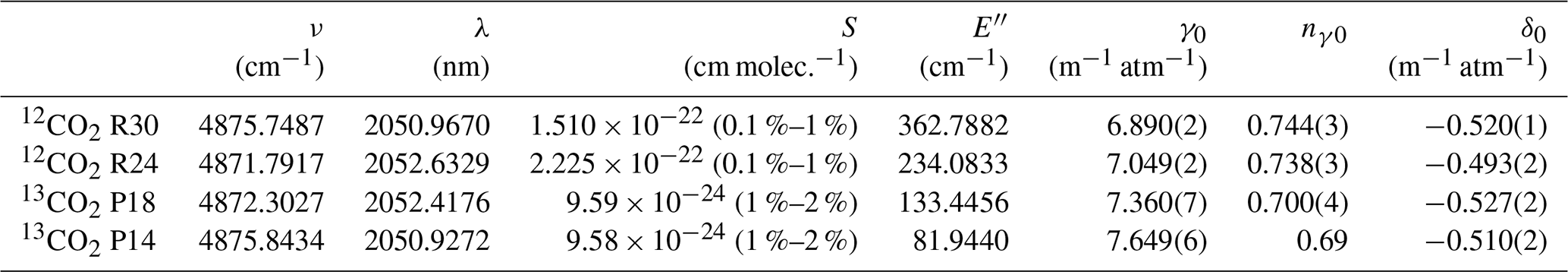
Fortunately, in the 2.05 µm band, the ¹³CO₂ line intensities and then ACS are larger by 1 order of magnitude that mitigates, partly, their non-optimal DAOD. Figure 1 shows ACS calculated with line intensities from HTRAN2020 database (Gordon et al., 2022) in the 2.06 µm spectral region. These were obtained with a multispectrum fitting approach using a modified Voigt line shape to include line mixing and quadratic speed dependence. This database has been improved for air-broadening, air-pressure shift coefficients and their temperature dependence with recent CRDS lab measurements for ¹²CO₂ (Mondelain et al., 2023) and for ¹³CO₂ absorption lines (Mondelain et al., 2025) (Table 1). The residuals obtained after the multi-spectrum fit procedure are usually lower than 0.05 % for the absorption lines considered in this study. Note that the isotopologue abundances taken from the spectroscopic database yield a ¹³CO₂/¹²CO₂ isotopic ratio of 0.011235 (https://hitran.org/docs/iso-meta/, last access: 12 November 2025) which differs from the VPDB's one. This creates a bias of −0.18 ‰ in δ¹³C. Water vapor absorption lines absorption cross-sections have been calculated using a Voigt line shape and HITRAN2020 database.

Table 1 Main ¹²CO₂ and ¹³CO₂ absorption line parameters used in this study. S: line intensity at 296 K weighted by standard isotopic abundance; E^′′: lower energy level of the transition; γ₀: air broadening coefficient at 296 K; $n_{{\mathit{\gamma }}_{\mathrm{0}}}$: temperature dependence exponent; δ₀: air-pressure shift coefficient at 296 K. Line intensity values and uncertainties are taken from HITRAN2020 database (Gordon et al., 2022). Values and uncertainties for γ₀, $n_{{\mathit{\gamma }}_{\mathrm{0}}}$, δ₀ are from Mondelain et al. (2023, 2025). One-sigma uncertainties are given in parenthesis in the unit of the last digit.

Using Table 1 and Fig. 1, we are able to calculate typical absorption coefficient due to ¹²CO₂ and ¹³CO₂ at the chosen wavelengths λ₁ and λ₂: ∼ 0.75 and ∼ 0.05 km⁻¹ respectively. From Eq. (1), the relative error of DIAL absorption measurement can be roughly written $\mathit{\sigma }\left({\mathit{\alpha }}_i\right)/{\mathit{\alpha }}_i\propto \mathrm{1}/\left({\mathit{\alpha }}_i\cdot \mathit{\delta }R\cdot {\text{SNR}}_i\right)$ where SNR_i is the λ_i lidar signal to noise ratio. Therefore, to obtain similar precision on DIAL absorption measurement at λ₁ and λ₂, SNR₂ > 15 SNR₁ which represents a huge instrumental effort. Comparing to Gibert et al. (2015) CDIAL set-up used for ¹²CO₂ measurement only, range and time resolution will have then to be reduced and the laser should run at higher pulse repetition frequency to obtain a larger SNR.

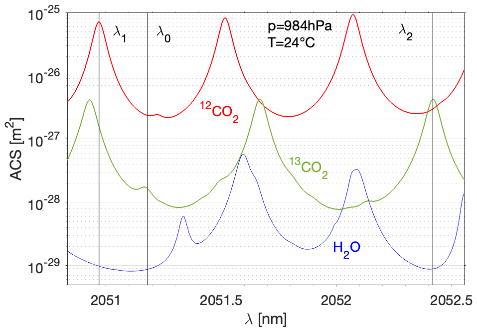
Figure 1 Absorption cross-section (ACS) for ¹²CO₂, ¹³CO₂ and H₂O for pressure 984 hPa and temperature 24 °C (Voigt profile). Isotopic ratio is taken into account. The DIAL wavelengths chosen in this work are indicated.

4 Experimental set-up

The lidar set-up is displayed in Fig. 2 and the technical specifications are gathered in Table 2. The laser set-up has been significantly modified since our DIAL CO₂ measurements (Gibert et al., 2015, 2018) following recent work on hybrid fiber/bulk amplifier in the 2 µm domain (Lahyani et al., 2021, 2024). Our current emitter uses a seeder module with three narrow linewidth external cavity laser diodes (special model CHEETAH from Sacher Lasertechnik). Both seeders, λ₁ and λ₂, are locked to ¹²CO₂ and ¹³CO₂ absorption line centers using two frequency reference systems (FRS) built with a 80 cm path gas cell filled with pure ¹²CO₂ at 20 hPa and ¹³CO₂ at 5 hPa respectively and a Pound-Drever-Hall (PDH) technique. Gas cell pressures have been chosen to have the narrowest line shape as possible while maintaining a transmission around 0.5. λ₀ is locked to λ₁ using a phase-locking loop and a beat frequency monitoring. The spectral precision of each wavelength presents an Allan deviation better than 1 MHz between 10 s and 10 min (Gibert et al., 2018). In addition, the accuracy of each wavelength is within 1 MHz. After a 4 × 1 double stage fibered switch (Agiltron) (measured cross-talk isolation larger than 45 dB), the seeder power is amplified through a CW Thulium doped fiber amplifier (TDFA) (model CTFA from Keopsys). The laser pulses are then shaped using an acousto-optic modulator AOM (model Brimrose – 50 MHz). An electro-optical modulator and a double-stage optical fibered-coupled switch (Agiltron – not represented in Fig. 2) is added to reject (by 50 dB) the long settling time CW power after the pulse. The pulse repetition rate is 6 kHz as a compromise to have a large number of samples and keep a sufficient Carrier to Noise Ratio (CNR). The wavelength switch is fixed at 60 Hz (switch every 100 pulses at fixed wavelength) as a compromise to limit switch disturbance on the measurements (switch cross-talk is limited to 30 dB) and keep identical atmospheric aerosol backscatter signal for the three wavelengths.

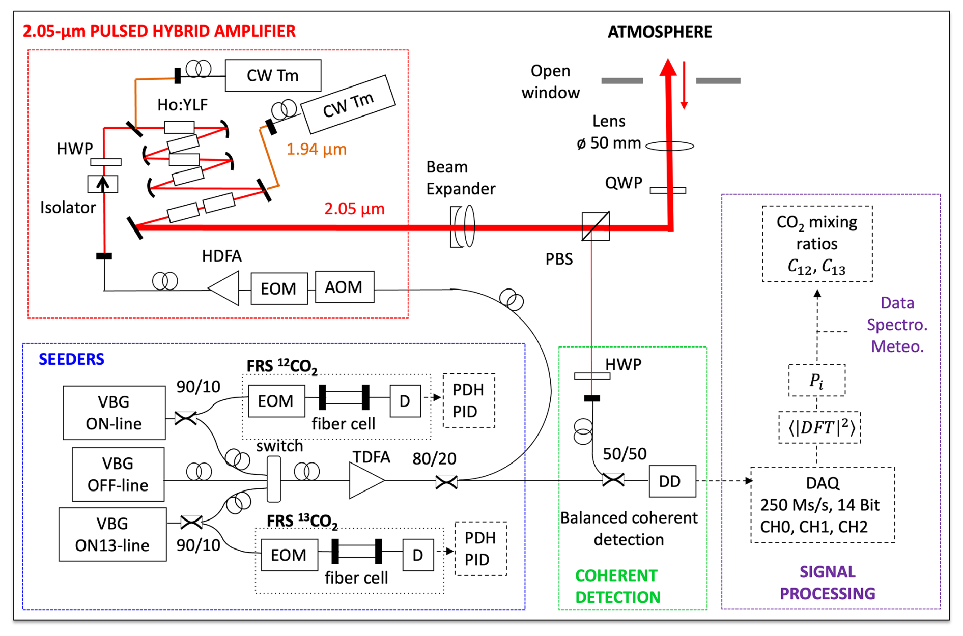
Figure 2 DIAL set-up for δ¹³C measurement. FRS: frequency reference system, EOM et AOM: electro and acoustic-optical modulators, HDFA and TDFA: Holmium and Thulium fiber amplifiers, VBG: volume Bragg grated laser diode, PDH: Pound-Drever-Hall, HWP and QWP: half and quarter wave plate, PBS: polarizer beam splitter. Signal processing: data acquisition system (DAQ) with 3 channels (CH0, CH1 and CH2) for the 3 wavelengths, real time range-gate Discrete Fourier Transform (DFT), backscatter power (P_i) at each wavelength and ¹²CO₂ (C₁₂) and ¹³CO₂ (C₁₃) mixing ratios computed with additional spectroscopic and in situ meteorological data.

Table 2 Key specifications of ¹²CO₂ and ¹³CO₂ DIAL system. Further details may be found in Gibert et al. (2018) and Lahyani et al. (2021, 2024).

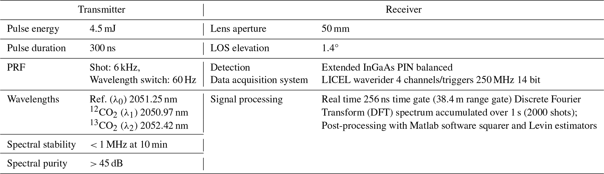
A custom Holmium pulsed fibered amplifier (model THALYS-2051nm-0.2W from Cybel) enables to deliver a maximum of 17 W peak power (∼ 5 µJ for a 300 ns pulse duration) without parasitic stimulated Brillouin scattering (SBS) effect. The laser pulses are then amplified in a free space multi-pass Ho:YLF amplifier. Six 0.5 %-Holmium doped 50 mm long Ho:YLF rods pumped by two 50 W linearly polarized Thulium fiber lasers (model TLR-50-1940-LP from IPG Photonics) are used to obtain a mean 27 W output power at 2.05 µm (4.5 mJ at 6 kHz). Both high cross-talk isolation from the double stage optical switch and high side mode suppression from the amplifiers (Lahyani et al., 2024) give an overall spectral purity larger than 45 dB. This laser architecture enables flexible characteristics of the laser: pulse duration, energy and repetition frequency (PRF). A coherent detection with a 50 mm diameter aperture lens (optimal heterodyne efficiency for horizontal measurement close to the surface over a distance of 2 km), a balanced extended InGaAs photodiode detection (Discovery Semiconductors Inc.) and a four channels data acquisition and real time signal processing system (model Waverider-250 from LICEL) completes the set-up.

The lidar has been installed on the second floor of the LMD building on Ecole Polytechnique campus (10 m height above the ground). The laser beam is sent quasi-horizontally into the atmosphere through an open window. A CRDS isotope and gas concentration analyser (PICARRO model G2131-i) made simultaneous continuous measurements of ¹²CO₂ and ¹³CO₂ mixing ratios. To complete the dataset, especially to compute the spectroscopic data, meteorological data were collected at the same height of the LMD lab 200 m away.

5 Atmospheric measurements

5.1 Absorption coefficient estimates

The signal processing is similar to the one described in Gibert et al. (2015). Real time processing consists in a 256 ns time gate (38.4 m range gate) Discrete Fourier Transform accumulation over 1 s (2000 shot averaging for each wavelength). Post-processing uses Matlab software with Squarer and Levin-like estimators to deliver atmospheric backscattered signal power and frequency at each wavelength (Gibert et al., 2006). The Doppler frequency shift is used to infer the radial wind speed at each wavelength (Gibert et al., 2015). Typical lidar profiles averaged over 10 min are displayed in Fig. 3.

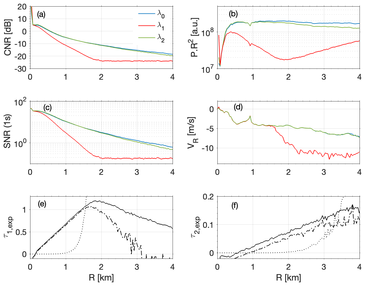
Figure 3 (a) Carrier to Noise Ratio (CNR) at each wavelength. (b) Range-corrected signal. (c) Signal to Noise Ratio for 1 s. (d) Radial wind speed. (e) DAOD calculated with signals from Levin-like estimator (solid line) and Squarer estimator (dashed and dotted line) for (e) λ₁ and (f) λ₂. The bias on DAOD calculated with Squarer estimates is indicated with the dotted line.

The CNR, CNR_i = $\left(P_i-P_{i,\mathrm{B}}\right)/P_{i,\mathrm{B}}$ where P_i,B is the noise power calculated using the integral of the power spectra of the last range gate of the lidar signal, is estimated for a bandwidth of 30 MHz (Fig. 3a). From the CNR and assuming that δR > cδt, where δt is the pulse duration, the lidar Squarer signal to noise ratio (SNR) may be estimated using (Killinger and Menyuk, 1981) (Fig. 3c):

$$\begin{array}{}\text{(7)}& {\text{SNR}}_i^{-\mathrm{1}}\cong N^{-\mathrm{0.5}}{\left(\mathrm{2}\mathit{\delta }R/\left(c\mathit{\delta }t\right)\right)}^{-\mathrm{0.5}}\left(\mathrm{1}+{\text{CNR}}_i^{-\mathrm{1}}\right),\end{array}$$

where N is the number of averaged spectrum (number of shots) at a given distance R.

A useful estimate of statistical and systematic error of DAOD (and then absorption) can be written from the SNR (Bösenberg, 1998; Gibert et al., 2008):

$$\begin{array}{}\text{(8)}& {\displaystyle }\text{SD}\left({\mathit{\tau }}_{i,\exp }\right)={\left({\text{SNR}}_i^{-\mathrm{2}}+{\text{SNR}}_{\mathrm{0}}^{-\mathrm{2}}\right)}^{-\mathrm{0.5}}/\mathrm{2}\text{(9)}& {\displaystyle }\mathit{\delta }\left({\mathit{\tau }}_{i,e\exp }\right)=\left({\text{SNR}}_{\mathrm{0}}^{-\mathrm{2}}-{\text{SNR}}_i^{-\mathrm{2}}\right)/\mathrm{4}\end{array}$$

Figure 3f shows that the fluctuations on DAOD seems to be far larger for τ_2,exp (¹³CO₂). The reason is that the relative error of τ_2,exp, being proportional to the optical depth, is larger by 1 order of magnitude compared to τ_1,exp, despite a larger SNR_i. Figure 3e and f also show that when the CNR and then the SNR decreases, the calculated DAOD is biased and underestimated as predicted by Eq. (9). Note that Levin-like estimator, which is actually used in this study, is significantly less sensitive to this bias and allows a longer range of measurement (Gibert et al., 2006).

To optimize the statistical error reduction on the DAOD, we look at the Allan deviation of each signal power at 500 and 1500 m and of the ratios $P_i/P_{\mathrm{0}}$ (Fig. 4). The lidar signal deviation at each wavelength does not decreases as the square root of time averaging except for very low CNR (CNR < −15 dB), i.e. for P₁ deviation at R = 1.5 km (Fig. 4b). The averaged lidar signal fluctuations are mainly due to the atmosphere. The Allan deviation of the ratios $P_i/P_{\mathrm{0}}$ shows that these fluctuations are correlated at each wavelength and their deviation decreases almost as the square root of the averaging time (but not entirely suggesting that some uncorrelated noise remains) and caps at few minutes of time averaging. Therefore, in this study, the signal processing consists in averaging the ratios of 1 s lidar signals up to 10 min and then take the logarithm in Eq. (1). The distance of useful DAOD measurement is chosen to have a negligible bias from Eq. (9). The bias due to potential negative values in the logarithm is also negligible with this process (Tellier et al., 2018). Note that the usual signal processing which consists to average the signals first up to 10 min and then take the ratio and the logarithm entails an increase of the DAOD standard deviation by a factor around two.

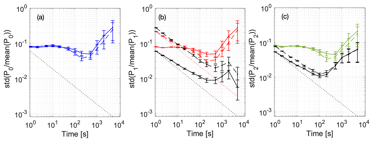
Figure 4 Allan deviation at R = 0.5 km (solid line) and R = 1.5 km (dashed line) for (a) λ₀, (b) λ₁ (red) and $P_{\mathrm{1}}/P_{\mathrm{0}}$ ratio (black), (c) λ₂ (green) and $P_{\mathrm{2}}/P_{\mathrm{0}}$ ratio (black). The dotted lines are indicated for the standard white noise deviation ($\mathrm{1}/\sqrt{\text{Time}}$).

The differential absorption coefficients, α_i,exp, are obtained with a Matlab bisquare linear fit on the DAOD which limits the weight of outliers with respect to the fitted line (Fig. 5). The regression is made over a distance of 1.3 km for α_1,exp (¹²CO₂) and 1.8 km for α_2,exp (¹³CO₂) while respecting several conditions: (1) the first points (R < 300 m) that are biased due to parasitic received CW emitted power after the emitted pulse (due to a roughly 1 µs long settling time of the AOM and switch) are discarded, (2) the farthest points that are biased due to low SNR (especially for λ₁) are also discarded, (3) a reasonable larger number of points for λ₂ (¹³CO₂) than for λ₁ (¹²CO₂) is used to mitigate the large statistical error of α_2,exp (due to lower optical depth) while keeping the same air mass (varying number of points have been tested to give credit to this hypothesis).

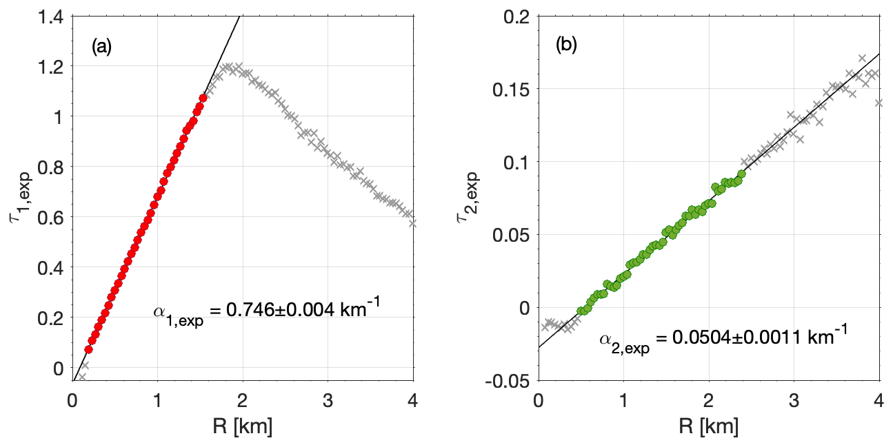
Figure 5 Differential optical depth for (a) λ₁ (¹²CO₂) and (b) λ₂ (¹³CO₂) and typical bisquare linear fit to estimate mean differential absorption coefficient. Colored dotted markers: points used for the fit; cross markers: outliers.

Given the error of C₁₃ absorption coefficient no range-resolved measurement is tested here at higher resolution, i.e. 200 m–10 min as such processing will only give noisy data where large CO₂ source will be hardly identified. Note anyway that range-resolved measurement for C₁₂ has been tested and gives similar results as in Gibert et al. (2015). Rather here, our goal is to get a useful precision on C₁₃ that will enables us to make a comparison with in situ data. Figure 5 shows an example of mean differential absorption coefficients estimates. With such conditions, the precisions on α_1,exp and α_2,exp are around 0.5 % and 2 %, respectively. Note that an offset spectral locking of λ₁ with respect to R30 ¹²CO₂ absorption line center is possible to have a similar useful distance of measurement than with λ₂, with the drawback of an increase of the statistical error though. Note also that the optical depths that we used here for CO₂ stable isotopologue measurements are similar to the ones used for DIAL H₂O stable isotopologue measurements (i.e. H${}_{\mathrm{2}}^{\mathrm{16}}$O and HD¹⁶O) at 1.98 µm (Hamperl et al., 2022) which enables to make some comparison in the following sections.

5.2 Meteorological data and absorption cross-section calculations

From meteorological data (p, T) and spectroscopic data we calculated the absorption cross section of each molecule (¹²CO₂, ¹³CO₂, H₂O) at each wavelength (Fig. 6). The main differential ACS variation is observed at λ₁ and is due to temperature diurnal cycle (around 0.2 % K⁻¹ at R30 ¹²CO₂ absorption line center) (Gibert et al., 2006).

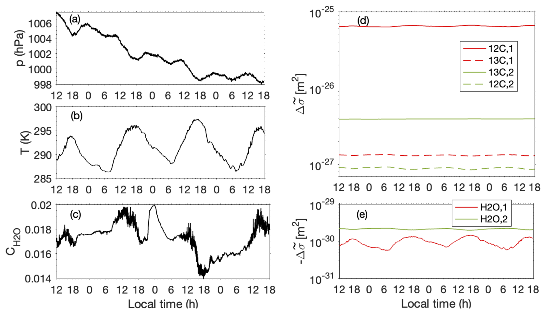
Figure 6 Meteorological data and differential ACS calculations. (a) Pressure (b) Temperature (c) H₂O mixing ratio (d) Differential ACS at wavelength 1 and 2 for ¹²CO₂ and ¹³CO₂ absorption lines and (e) for H₂O. Note that, as for Fig. 1, ¹³CO₂ ACS are multiplied by the VPDB isotopic ratio, i.e. 0.011237. Native in situ meteorological data have a time resolution of 1 min. Differential ACS are computed at the time resolution of Lidar measurements, i.e. 10 min.

5.3 Precision budget

The relative error of mixing ratio estimates results from the different parameters in Eq. (3): (1) the statistical error for absorption coefficient estimates (Fig. 5) and from its correction due to H₂O absorption (Eq. 4), (2) the uncertainty in differential ACS calculations which comes from uncertainties in meteorological data (mainly temperature) along the Lidar LOS and wavelengths position uncertainty, (3) the uncertainty in dry air density calculations mainly driven by C${}_{{\mathrm{H}}_{\mathrm{2}}\mathrm{O}}$ and T uncertainties along the Lidar LOS (the error due to pressure fluctuations is neglected). The relative error of each parameter is reported in Table 3. The uncertainties due to temperature fluctuations and water vapor along the line of sight of the Lidar are estimated from in situ data Allan deviation at 10 min, i.e. over the DIAL accumulation time. For the whole acquisition time (Fig. 6), the Allan deviation for T and C${}_{{\mathrm{H}}_{\mathrm{2}}\mathrm{O}}$ is respectively 0.18 K (< 0.07 %) and 1.3 × 10⁻⁴ (< 0.9 %). These mean relative errors are used to estimate the errors of the differential ACS assuming a Lorentzian absorption line shape and on the dry air density. Note that the relative error of mixing ratio due to temperature fluctuations in Table 3 accounts both from the differential ACS and the air density (Gibert at al., 2008). The relative error of α_i and then on mixing ratios due to water vapor absorption correction (Eq. 4) is calculated using an upper bound for water vapor absorption contribution in α_i,exp from Fig. 6, which amounts to 0.1 % of α_1,exp, and 1.7 % of α_2,exp.

Table 3 Statistical errors of ¹²CO₂ (C₁₂) and ¹³CO₂ (C₁₃) mixing ratios.

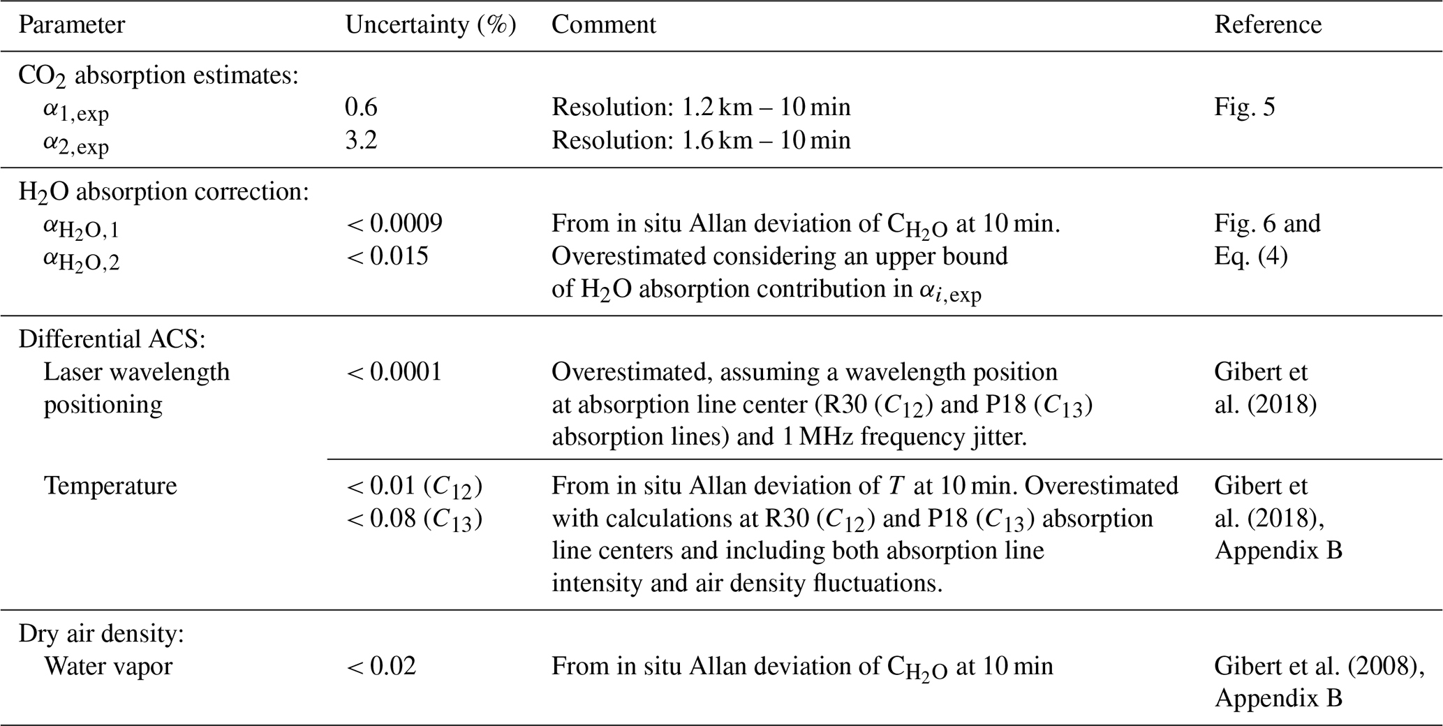
Table 3 shows that the uncertainty on mixing ratio estimates is mainly driven by the statistical error for absorption coefficient estimates from lidar backscatter signals. ¹³CO₂ mixing ratio estimate is also more sensitive to (1) water absorption correction due to a smaller absorption optical depth at wavelength 2 and (2) temperature fluctuations due to a less adapted energy level of the P18 transition than for ¹²CO₂ mixing ratio estimate. Although the DIAL system used for water vapor isotopologue measurements in Hamperl et al. (2022) is very different (direct detection DIAL), similar uncertainties were obtained for absorption coefficient estimates, i.e. 0.5  % for H₂O and 2.0 % for HDO for a time and space resolution of 25 min and 600 m at a mean distance of 400 m, showing that the measurement performances are driven, in both experiments, by the lowest optical depth of the stable isotopologues. However, a main difference of the two experiments concerns the spectral characteristics of the 2 µm emitters as the wavelength position precision contributes significantly in the error budget in Hamperl et al. (2022) whereas it has a negligible impact in our case.

5.4 Accuracy budget

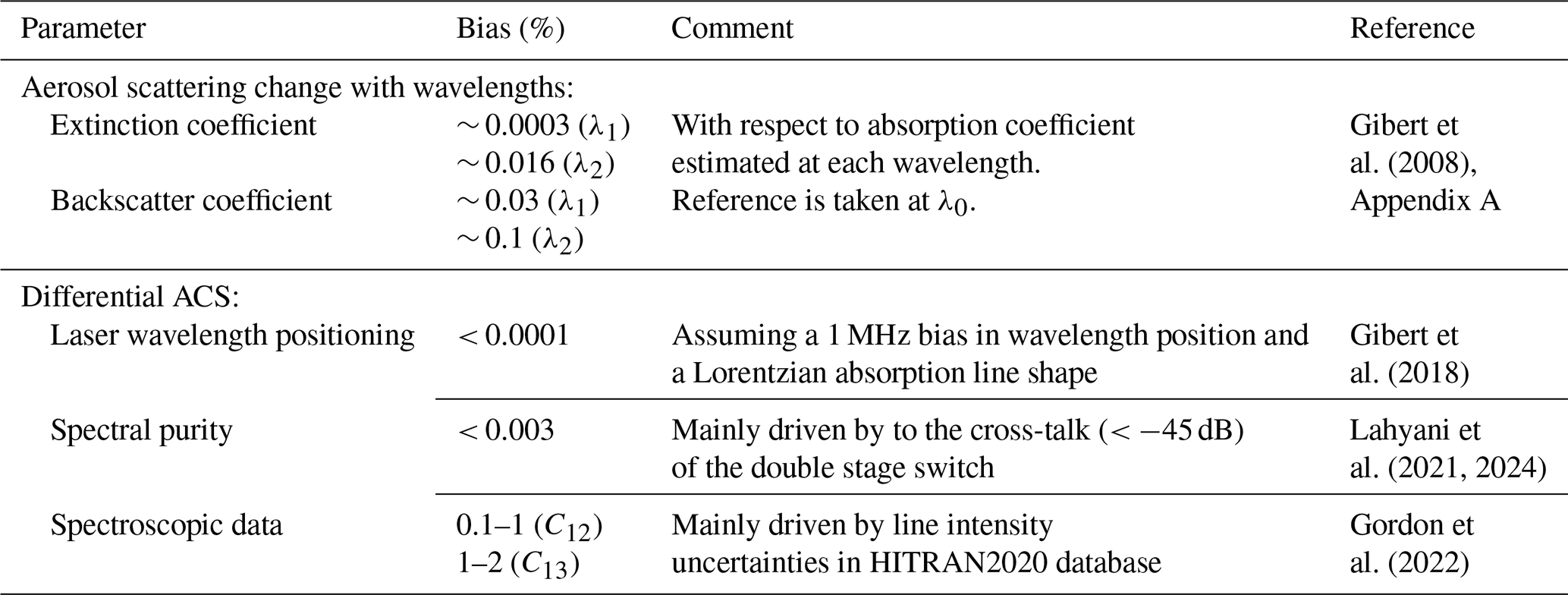
At the current point of our understanding, the systematic errors in DIAL ¹²CO₂ and ¹³CO₂ mixing ratios comes from: (1) a statistical bias that is corrected using Eq. (9), (2) approximations in the DIAL equation (Eq. 1) which neglects spectral variation of aerosol extinction and backscatter coefficients especially for λ₂ (1.2 nm gap with λ₀), (3) instrumental characteristics of the DIAL emitter such as the absolute wavelength positions and the spectral purity, (4) spectroscopic data.

Given the 1.2 nm wavelength difference in DIAL measurements of ¹³CO₂, one may wonder what is the aerosol backscatter and extinction coefficient differences over such a spectral range. This has actually been studied and quantified in Appendix A of Gibert et al. (2008). A Mie scattering code for homogeneous spherical particles (Mätzler, 2002) accounting for typical aerosol optical depth and size distribution in the suburban area of Palaiseau and a wide range of relative humidity showed an error of CO₂ absorption coefficient of 2 × 10⁻⁷ m⁻¹ from the backscatter coefficient and 2 × 10⁻⁹ m⁻¹ from the extinction for a wavelength difference of 0.3 nm at 2.06 µm. Assuming that we can describe the wavelength dependance of extinction (and backscatter coefficient) with the Angström exponent: δα_i = ${\mathit{\alpha }}_{p,\mathrm{0}}\left[\mathrm{1}-{\left({\mathit{\lambda }}_{\mathrm{0}}/{\mathit{\lambda }}_i\right)}^{a^{\mathrm{0}}}\right]$ (Weitkamp, 2005). With an assumed suburban a⁰ ∼ 1, we obtain δα₁ = 1.4 × 10⁻⁴ α_p,0 for |λ₁−λ₀| = 0.3 nm and δα₂ = 5.6 × 10⁻⁴ α_p,0 for |λ₂−λ₀| = 1.2 nm which keeps the numbers calculated above from Gibert et al. (2008) in the same order of magnitude, i.e. 8 × 10⁻⁷ m⁻¹ from the backscatter and 8 × 10⁻⁹ m⁻¹ from the extinction coefficients. These numbers have to be compared to typical CO₂ absorption coefficients α₁ (∼ 7.5 × 10⁻⁴ m⁻¹) and α₂ (∼ 5.0 × 10⁻⁵ m⁻¹) to obtain the relative biases in Table 4. Our bias estimation shows that the aerosol backscatter spectral difference could have a significant impact on ¹³CO₂ mixing ratio estimates (potential bias of 0.1 %) if significant aerosol gradients occur in the atmosphere (plume, boundary layer interface). Other systematic errors from the spectroscopic data and DIAL emitter have been quantified as well in Table 4.

Table 4 Assessment of potential systematic errors of ¹²CO₂ (C₁₂) and ¹³CO₂ (C₁₃) mixing ratios.

In order to quantify the actual biases on C₁₂ and C₁₃ estimates, we considered the direct problem. In situ differential absorption coefficients for both wavelength 1 and 2 are computed using meteorological, spectroscopic data and in situ PICARRO G2101-i isotopic gas analyzer measurements of ¹²CO₂ and ¹³CO₂ mixing ratios. Figure 7 shows the comparison between lidar and in situ estimates. A “good” (with respect to expected representativity error) correlation coefficient of 0.80 and 0.82 are calculated for α₁ and α₂, respectively. However, a linear fit shows both a different amplitude of variation and a bias that are not explained up to now, neither by the signal processing nor by the potential biases listed in Table 4. The coefficients of the linear fit remain constant within the uncertainties over the 4 d of measurements. These biases are likely due to the long settling time of the emitted pulse shaped by the AOM (Fig. 2). As seen in Fig. 3a, a part of the emitted pulse (and the remaining power after it) is reflected by the optics after the polarizer (Fig. 2) which may create a different bias on atmospheric backscattered power at each wavelength. To pursue the analysis of the lidar measurements, especially from the statistical point of view, we decided to correct the lidar absorption coefficients by these linear fit coefficients keeping in mind that further work will be needed on lidar measurements biases.

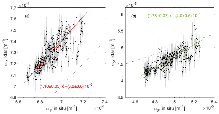
Figure 7 Comparison between lidar and in situ differential absorption coefficient (from meteorological, spectroscopic and gas analyzer data) for wavelength 1 (¹²CO₂) (a) and 2 (¹³CO₂) (b). The dotted line is for α_i,lidar = α_i,in situ.

6 Discussion

6.1 Diurnal variations of ¹²CO₂ and ¹³CO₂ in the atmospheric surface layer

To show the current performances of CDIAL CO₂ isotopic measurements, we report almost 70 h of lidar C₁₂ and C₁₃ mixing ratio measurements in the surface layer at approximately 15 m height above Ecole Polytechnique campus (Fig. 8). The lidar reflectivity and the radial wind speed along the line of sight (LOS) of the lidar are also displayed. The diurnal cycles of lidar C₁₂ and C₁₃ estimates follow the in situ data with two exceptions on 18 September (6 h) and 20 September (10 h) that correspond to changes in radial wind speed and direction (Fig. 8b and c). Large differences between in situ and lidar measurements are then explained by different spatial representativity. Other major differences are also observed on the evenings, 18 September (20 h) and 19 September (20 h). These correspond likely to anthropogenic plumes (evening road traffic) that are not well mixed during the evening transition and are located hundreds of meters far from the LMD building where is the in situ gas analyzer (R = 0 km). The ¹²CO₂ anomaly magnitude of these plumes (10–20 ppm) is similar to what was measured in Gibert et al. (2015). When the atmospheric boundary-layer is well mixed by turbulence (seen with fluctuated values of V_R along the LOS, 12–18 h in local time) the agreement (within the error bars) between lidar and in situ sensor measurements is excellent, as expected.

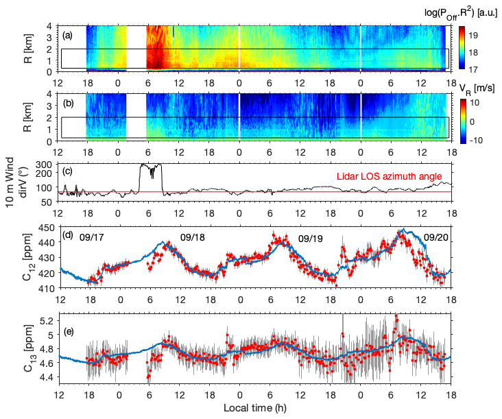
Figure 8 C₁₂ and C₁₃ lidar measurements. (a) Lidar reflectivity for wavelength 0 and associated. (b) Lidar radial wind speed. (c) In situ horizontal wind direction (dirV) at 10 m and lidar line-of-sight (LOS) azimuth angle. (d) C₁₂ and (e) C₁₃ lidar mixing ratio measurements (markers). The solid line corresponds to in situ PICARRO G2101-i analyzer measurements. Space resolution for lidar C₁₂ and C₁₃ measurements is around 1.0–1.3 and 1.5–1.8 km respectively depending the level of the signal power (a). Time resolution is 10 min. Error bars are calculated from α_i,exp estimates (Fig. 5).

The natural change in lidar reflectivity and therefore CNR and SNR entails a variation of the maximum distance of measurements (to avoid optical depth biases) and then of the resolution of lidar differential absorption estimates along the 70 h: 1.0–1.3 km for C₁₂ and 1.5–1.8 km for C₁₃. The precision of lidar mixing ratio estimates changes as well and ranges between 1.3 and 6.4 ppm for C₁₂ (median value: 2.3 ppm (0.6 %)) and 0.06 to 0.4 ppm for C₁₃ (median value: 0.15 ppm (3.2 %)).

6.2 Current status and future prospective concerning δ¹³C lidar estimates

From Eq. (5), we calculated the CO₂ isotopic ratio δ¹³C both for in situ and lidar measurements and report the 70  h data in a Keeling plot (Fig. 9a). A least-squares fit on the in situ data results in a mean δ¹³C_source = −26 ‰ both a result of vegetation respiration and traffic road anthropogenic emissions in this suburban area (Lopez et al., 2013; Widory and Javoy, 2003). The lidar data gave a similar value although the large uncertainty (260 %) prevents us to obtain any conclusion. Using Eq. (5) we can calculate the statistical error of δ¹³C:

$$\begin{array}{}\text{(10)}& \text{SD}\left({\mathit{\delta }}^{\mathrm{13}}\mathrm{C}\right)\cong \sqrt{{\displaystyle \frac{\text{var}\left(C_{\mathrm{12}}\right)}{C_{\mathrm{12}}^{\mathrm{2}}}}+{\displaystyle \frac{\text{var}\left(C_{\mathrm{13}}\right)}{C_{\mathrm{13}}^{\mathrm{2}}}}}\end{array}$$

From Eq. (10) we understand that the lidar error of δ¹³C is driven by the statistical error of C₁₃ lidar mixing ratio estimate.

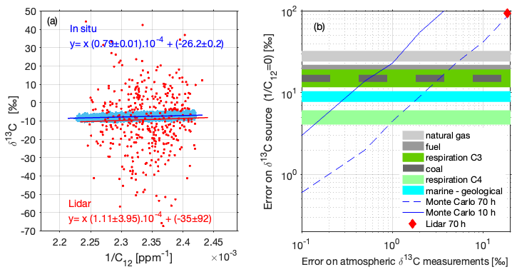
Figure 9 (a) Keeling plot for in situ gas analyzer and CDIAL measurements. (b) Monte Carlo simulations of the δ¹³C_source error estimate (time resolution is 10 min) using in situ gas analyzer as the truth and random additional noise on δ¹³C measurements. Lidar error of δ¹³C_source estimate with 70 h of measurements is indicated as well as δ¹³C_source geophysical typical anomalies for natural gas, fuel, coal anthropogenic emissions, C₃ and C₄ plant respiration and marine or geological source with respect to standard atmospheric mixed air δ¹³C (9 ‰).

To predict the future performances of optimized lidar system for δ¹³C measurement, we made Monte Carlo numerical simulations assuming the same spread of $\mathrm{1}/$ C₁₂ in situ data collected during this field experiment and adding some increasing random noise on δ¹³C in situ values. The goal was to infer an error threshold of a future optimized lidar system to see geophysical δ¹³C sources (Fig. 9b). Typical δ¹³C_source anomalies with respect to a mixed air reference of 9 ‰ have been reported on Fig. 9b for comparison. The current lidar δ¹³C_source error is also reported and agrees with a Monte Carlo error simulation. If we keep the same number of points that were used in this study (70 h of measurements with 10 min time resolution) we understand that a threshold lidar error should be around 7 ‰, 3 ‰, 2 ‰ and 1 ‰ to detect respectively natural gas, coal/fuel/C₃ plant respiration, marine/geological and C₄ plant respiration δ¹³C_source anomalies (Widory and Javoy, 2003). Given that such detection should be made ideally during a single night (10 h acquisition) or for anthropogenic plumes (typical minute time scale), the precision to reach is even more challenging (< 1 ‰). Concerning our current lidar system, relying on a coherent detection for ¹³CO₂ DIAL measurement, the SNR should be increased by at least 20 dB to obtain a better spatial resolution and a precision around 0.1 %, which seems to be technically unreachable with the present coherent detection. However, some hope still exists with direct detection DIAL using an internally amplified photodetector such as HgCdTe avalanche photodiodes (Sun et al., 2014; Dumas et al., 2017) or superconducting nanowire single-photon detectors (SNSPD) (Yue et al., 2022).

7 Conclusion

A first investigation of range-resolved DIAL for the measurement of CO₂ isotopic composition in the atmosphere has been presented. A three wavelengths CDIAL lidar was developed for simultaneous measurements of ¹²CO₂ and ¹³CO₂ in the 2 µm spectral domain. The spectroscopic database has been updated with recent experimental data with outstanding accuracy and precision. The LMD CDIAL system has also been upgraded since 2015 and relies now on a new 27 W hybrid fiber/bulk multiple wavelength laser at 2 µm that offers similar performances but a better flexibility with respect to pulse energy, duration and rate tuning. A specific optimized configuration for this study provides a three wavelengths emission with 4.5 mJ, 300 ns and 6 kHz pulses. The CDIAL system was used to make first range-resolved measurements of ¹²CO₂ and ¹³CO₂ absorption in the atmospheric surface layer above the suburban area in the south of Paris. Typical performances of the instrument (median values along 70 h of measurement) with 10 min of time averaging show: (1) a precision around 0.6 % for 1.2 km range resolution for ¹²CO₂ mixing ratio (2) a precision around 3.2 % for 1.6 km range resolution for ¹³CO₂ mixing ratio. In situ co-located gas analyser measurements were used to correct for biases that are explained neither by the spectroscopic database accuracy nor the signal processing and will need further investigation. Then, differences in ¹²CO₂ and ¹³CO₂ mixing ratio anomalies between in situ and CDIAL made sense as the results of dynamical processes and different sounding representativity in the atmosphere. Once again, the simultaneous radial wind speed ability of the CDIAL system was critical to explain geophysical CO₂ variability in the surface layer linked to surface emissions that are not fully mixed.

Both limited precision and accuracy of the current set-up prevent us to make useful geophysical measurements of the isotopic ratio δ¹³C in order to characterize the sources of CO₂. Nevertheless, both in situ and CDIAL measurements were used to make a state of the art for current lidar ability to provide δ¹³C measurements in the atmosphere with respect to geophysical expected anomalies and to predict the necessary performances of a future optimized instrument. Monte Carlo simulations showed that an increase of the instrument SNR by 2 orders of magnitude is necessary to get a useful geophysical precision better than 1 ‰ on δ¹³C. This precision is fully limited by the precision on DIAL ¹³CO₂ absorption measurement that suffers from a small absorption coefficient around 0.05 km⁻¹ in the 2 µm spectral domain (compared to 0.75 km⁻¹ for ¹²CO₂). Despite such increase of SNR seeming to be out of range for a coherent DIAL system with reasonable range and time resolution, such performances are still achievable with a direct detection DIAL and this will be tested in a future work.