Deployment and evaluation of a low-cost sensor system for atmospheric CO₂ monitoring on a sea–air interface buoy

Direct in-situ observation of marine CO₂ concentrations is crucial for estimating air–sea CO₂ fluxes, yet such observations remain scarce. Drawn on experiences from urban CO₂ monitoring and buoy-based measurements, this study deployed a sea–air interface buoy platform in the northern South China Sea, near Maoming, Guangdong Province, China. This platform was equipped with three low-cost SenseAir K30 sensors to enable continuous atmospheric CO₂ measurement. This paper presents the first detailed account of the methodology, encompassing hardware design, environmental corrections, land-based validation tests, offshore deployment procedures, and initial observational results. These findings thus provide valuable insights for advancing marine CO₂ observations practices. To mitigate the impacts of temperature, humidity, and pressure on sensor readings – while simultaneously compensating for zero-drift – an environmental correction method was implemented. This approach significantly improved data accuracy: after 1 min temporal averaging of raw data and a subsequent 1 h moving average, the root mean square error was reduced from 8.03 to 3.64 ppm in land tests and from 24.26 to 1.59 ppm in marine observations. Importantly, this level of precision meets the requirements for resolving sea surface CO₂ dynamics (∼ 420–480 ppm). Observed concentrations were consistent with HYSPLIT-simulated long-range atmospheric transport, revealing the stable and homogeneous nature of the marine atmospheric boundary layer, with diurnal variations of approximately 3 ppm, and capturing localized or short-term fluctuations due to terrestrial carbon sources. These results demonstrate the effectiveness of the method, offering a low-cost, high-density solution for marine atmospheric CO₂ monitoring and providing key inputs for inversely estimating ocean carbon sink.

1 Introduction

Since the Industrial Revolution, less than half of the carbon emitted into the atmosphere by human activities remains in the atmosphere (Friedlingstein et al., 2020; Costa et al., 2023), highlighting the pivotal role of terrestrial and ocean sinks in regulating atmospheric CO₂ concentrations. From 2013 to 2022, the ocean absorbed and stored CO₂ approximately 26 % of total anthropogenic CO₂ emissions (Friedlingstein et al., 2023). The ocean stores a vast amount of CO₂, with inorganic carbon reservoir approximately 50 times greater than those in the atmosphere (Sabine et al., 2004). Therefore, studying oceanic CO₂ sources and sinks is crucial for developing mitigation strategies and mitigate climate change. The most widely and extensively applied, and long-established method for ocean carbon sink investigation involves measuring the partial pressure difference of CO₂ (ΔpCO₂) across the air–sea interface (Song et al., 2023). Continuous observations used to calculate the air–sea CO₂ flux, providing the most direct characterization of the ocean carbon cycle system (Wanninkhof et al., 2019; Song et al., 2023).

Owing to the past several decades of continuous observations, a large amount of sea surface pCO₂ data has been accumulated, yet it remains insufficient relative to the vast ocean area. The Surface Ocean CO₂ Atlas (SOCAT v2024) revealed that the ocean area covered by monthly CO₂ measurements has decreased by nearly half since 2017, reflecting the decline in global open-ocean CO₂ observation capacity (Bakker et al., 2024). Although recently studies have increasing employed artificial intelligence and big data technologies to investigate the dynamics of ocean carbon sinks (Landschützer et al., 2013; Xu et al., 2019; Yu et al., 2023), the fundamental limitation of in-situ field observation remains unresolved. Due to the limited spatial and temporal coverage of ΔpCO₂ measurements, as well as uncertainties in wind forcing and transport velocity parameterization, the uncertainty in global and regional fluxes estimated from ΔpCO₂ measurements can reach up to ± 50 % (Wanninkhof et al., 2013; Rhein et al., 2013). In addition to ΔpCO₂ data, air–sea CO₂ fluxes can also be estimated using a top-down inversion method that integrates atmospheric CO₂ concentrations with atmospheric transport models (Jacobson et al., 2007; Wanninkhof et al., 2019). Spatial and temporal variations in atmospheric CO₂ concentrations reflect the pattern of sources and sinks across large spatial scales. Consequently, top-down atmospheric inversion methods are suitable for assessing global and regional CO₂ fluxes and are currently widely adopted to estimate CO₂ emissions from fossil fuels and carbon sinks in terrestrial ecosystems (Piao et al., 2022; Han et al., 2024). However, due to the sparse sampling of CO₂ concentration over the open ocean, significant uncertainties persist in those flux estimations, limiting its applicability (Rödenbeck et al., 2006; Wanninkhof et al., 2019). In summary, the scarcity of marine atmospheric CO₂ concentration observations is the primary obstacle to accurately quantify the oceanic carbon sink.

For marine atmosphere, buoy observations excel at meeting the requirements of expanding field observation coverage and significantly increasing data volume compared to research vessel observations constrained by voyage frequency, range, and cost, or satellite observations limited by operational cycles and atmospheric conditions (e.g., clouds, aerosols). Currently, both the ARGO Global Ocean Observing System and the Southern Ocean Carbon and Climate Observation and Modeling (SOCCOM) project have proposed utilizing buoys for seawater CO₂ observations (Sarmiento et al., 2023), but none of them have conducted atmospheric CO₂ concentrations over the ocean. Urban CO₂ monitoring efforts provide valuable experience for selecting CO₂ observation instruments suitable for deployment on buoys. In recently years, high-density monitoring networks based on low-cost CO₂ sensors have been established in numerous cities worldwide (Karion et al., 2020), as supplements to the land-based observations from the sites within the World Meteorological Organization's (WMO) Global Atmosphere Watch Programme (GAW). For instance, Shusterman et al. (2016) established a CO₂ observation network (BEACO₂N) which consists of 34 sensors in and around Oakland, California. After applying environmental parameter and drift corrections, the network achieved an accuracy of ± 1.2–2.0 ppm for 1 min average dry-air concentrations between, effectively capturing CO₂ variations across multiple temporal scales in urban areas and abnormal short-term CO₂ emission events. Delaria et al. (2021) further corrected the temperature-dependent zero bias of the BEACO2N sensor, reducing the error to 1.6 ppm or less. Han et al. (2024) established a 134-station SenseAir K30 sensor observation network and developed a CO₂ calibration system. Data accuracy was enhanced through averaging raw observations, environmental corrections, and calibration with standard gases. After applying long-term drift correction, the sensors (SENSE – IAP) maintained a root mean square error (RMSE) of 2.4 ± 0.2 ppm after 30 months of operation (Cai et al., 2025). Compared to high-precision instruments, low-cost sensors exhibited relatively lower accuracy (several ppm versus ∼ 0.1 ppm) but at drastically reduced cost (under USD 15 000 versus over USD 150 000). This cost-performance balance enables the construction of dense observation networks to reveal significant spatial variations of CO₂ induced by emission sources, vegetation carbon sinks, and meteorological conditions (Shusterman et al., 2016; Bakker et al., 2024; Han et al., 2024; Cai et al., 2025).

Considering the advantages of low-cost sensors in land-based CO₂ monitoring and inversion, and the relative maturity of buoy-based observation technologies, we designed a sea–air interface buoy platform equipped with SenseAir K30 sensors (SenseAir AB, Delsbo, Sweden) in the coastal waters off Maoming, Guangdong, China, and evaluated its performance in monitoring marine atmospheric CO₂ concentration. Satisfying measurement accuracy was obtained after instrumental calibration, data processing, and correction strategies, validating the feasibility of marine CO₂ monitoring with low-cost sensors. Here we presented the preliminary results of the buoy-based low-cost sensor system for atmospheric CO₂ monitoring at the sea–air interface. Section 2 introduces the instruments and data correction methods; Sect. 3 presents the results of the land-based experiments for calibration and correction; Sect. 4 demonstrates a short-term marine observation case study; and Sect. 5 presents and discusses the results of post-deployment laboratory validation of the sensors.

2 Data and Methods

2.1 Instruments and observation site

This study employed a low-cost sensor system integrating three CO₂ Sensor Modules (referred to as CM1, CM2, and CM3) (Fig. 1c), capable of simultaneously measuring atmospheric CO₂ concentration and meteorological parameters including temperature, pressure, and humidity. Each CM integrates a CO₂ sensor, environmental parameter sensors, and a Micro-controller Unit (MCU) processor onto a single circuit board housed within a waterproof cube enclosure. Three CM modules are individually mounted in cylindrical housings bolted to a cube enclosure, with silicone seals at the connection points. Both sides and the bottom of the individual housings are wrapped with a membrane that is both breathable and waterproof, ensuring the CMs can operate normally in a marine environment. The CM feature an open-type design that allows ambient air to flow directly through the sensing chamber, without a sealed sampling volume typical of high-precision analysers. The sensors are paired with a data acquisition instrument, and data is collected by a micro-processor named BeagleBone Green Wireless (BBGW) and transmitted back to the server via 4G communication from the base station.

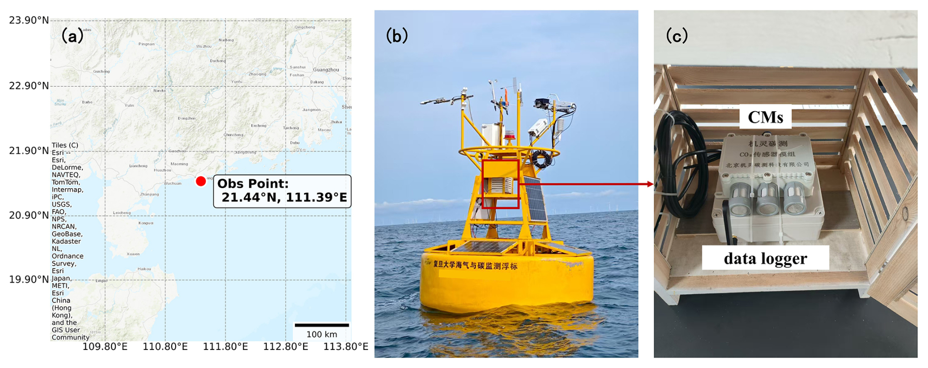
Figure 1 Deployment and performance evaluation of buoy-mounted sensors for marine atmospheric CO₂ observation. (a) Location of the offshore observation site. Basemap: Esri World Topographic Map | Powered by Esri (https://server.arcgisonline.com, last access: 9 September 2025). (b) On-site scene of the offshore buoy during observation. (c) Schematic of the CO₂ sensor modules (CMs), data logger, and Stevenson screen.

The CO₂ sensor is the K30 sensor module from SenseAir of Sweden, operating on a non-dispersive infrared principle (NDIR). Compared to other low-cost sensors (such as the COZIR Environmental Sensor (CO₂Meter, Inc., Orlando, FL, USA) and Telaire T6615 (Amphenol Advanced Sensors, USA)), it demonstrates higher raw accuracy, with ± 30 ppm ± 3 % (Martin et al., 2017), with a measurement range of 1–10 000 ppm and a resolution of 0.01 ppm, featuring easy configuration and maintenance-free operation. To account for the influence of external environmental variations on the K30 sensor's response, the CM is equipped with a BME680 sensor (Bosch Sensortec GmbH, Reutlingen, Germany) that simultaneously monitors temperature (T, °C), relative humidity (RH, %), and atmospheric pressure (P, hPa) of the internal air mass. The measurement accuracies are ± 0.1 °C, ± 3 %, and ± 0.6 hPa, with corresponding resolutions of 0.01 °C, 0.01 %, and 0.01 hPa, respectively. These measurements enable real-time correction of the CO₂ response values for environmental parameters, thereby enhancing the overall accuracy of the observations. The CMs adopt a standard RS485 output mode and are powered by the buoy's 12 V DC battery, operating continuously with a 2 s sampling interval. In the marine environment, pitching, strong winds, wave impacts, and rainy conditions are common. Combined with the high humidity and salinity of surface air, these factors often cause condensation and salt deposition on instrument surfaces. To mitigate these effects, the sensors and data logger were connected and securely mounted inside a Stevenson screen (Fig. 1c), which was installed near the buoy's center of gravity within the supporting frame (Fig. 1b), at an approximate height of 3 m above the sea surface, to provide a relatively stable observation environment.

The sea–air coupled monitoring buoy system is composed of a buoy platform and a land-based station (Fig. 2). The buoy consists of a buoy body, mooring system, sensors, data acquisition system, power system, safety system, and communication system. Real-time data transmission between the buoy and shore station is achieved via BeiDou (Fig. 1b). The buoy body has a diameter of 3 m, a depth of 0.9 m, and a total height exceeding 5 m. The power system comprises high-capacity, compact, rechargeable batteries, and solar panels. The batteries are housed within the instrument compartment, while solar panels are mounted around the buoy tower. These panels charge the batteries, supplying a single operating voltage to the buoy system. The system can sustain normal power supply to the buoy observation system for 15 consecutive days of overcast or rainy weather, ensuring continuous and reliable operation even under severe sea conditions. The buoy data communication system employs dual-mode Beidou and Iridium satellite communication, with redundant data transmission to ensure an effective data reception rate of better than 95 %. The shore station reception and processing system features reception, post-processing, and report generation capabilities, enabling modification and configuration of parameters such as buoy sampling frequency and transmission cycle. It also provides low-voltage, water ingress, and displacement alarm functions for buoys.

Figure 2 Schematic diagram of a deep-sea air–sea coupled monitoring buoy system.

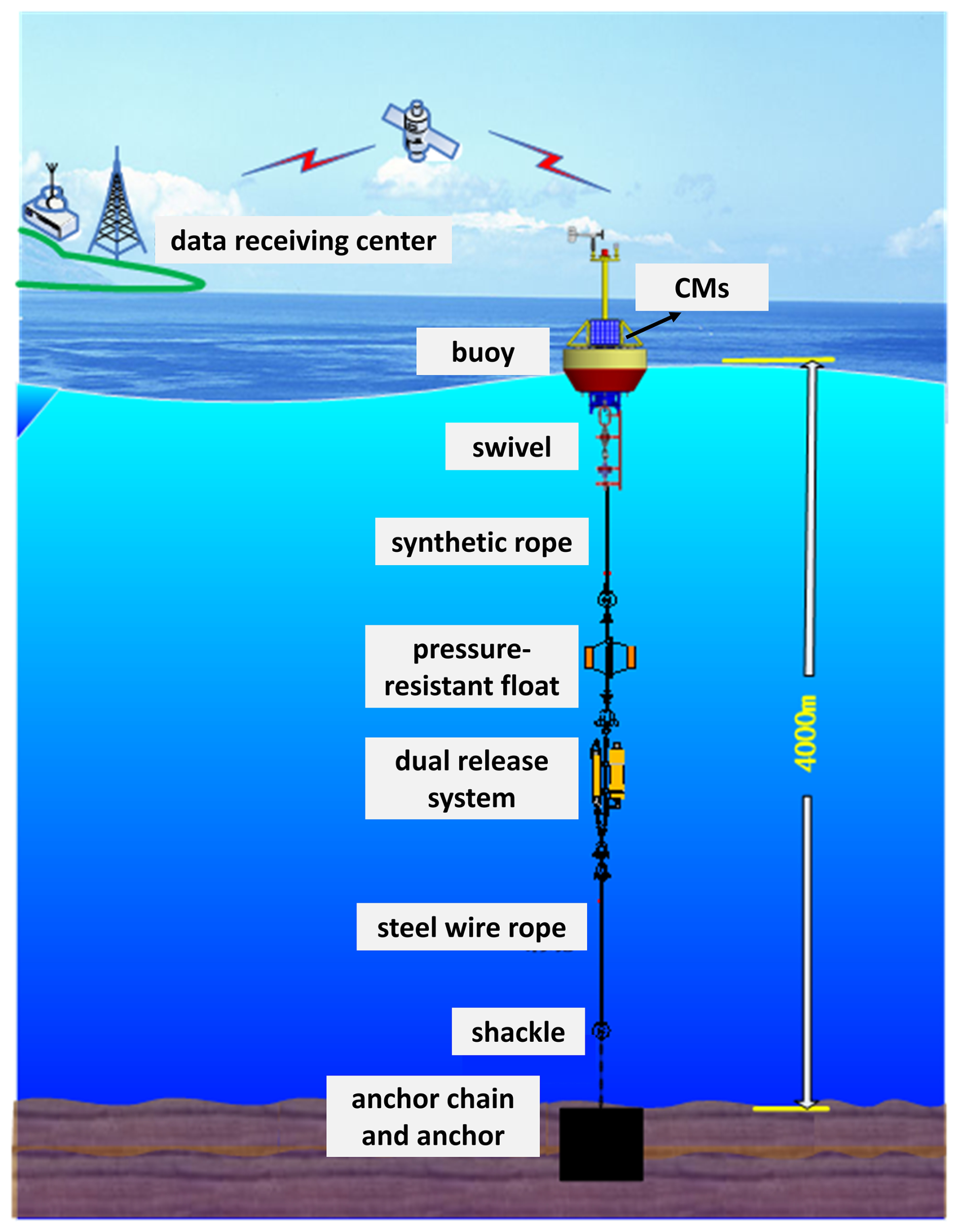
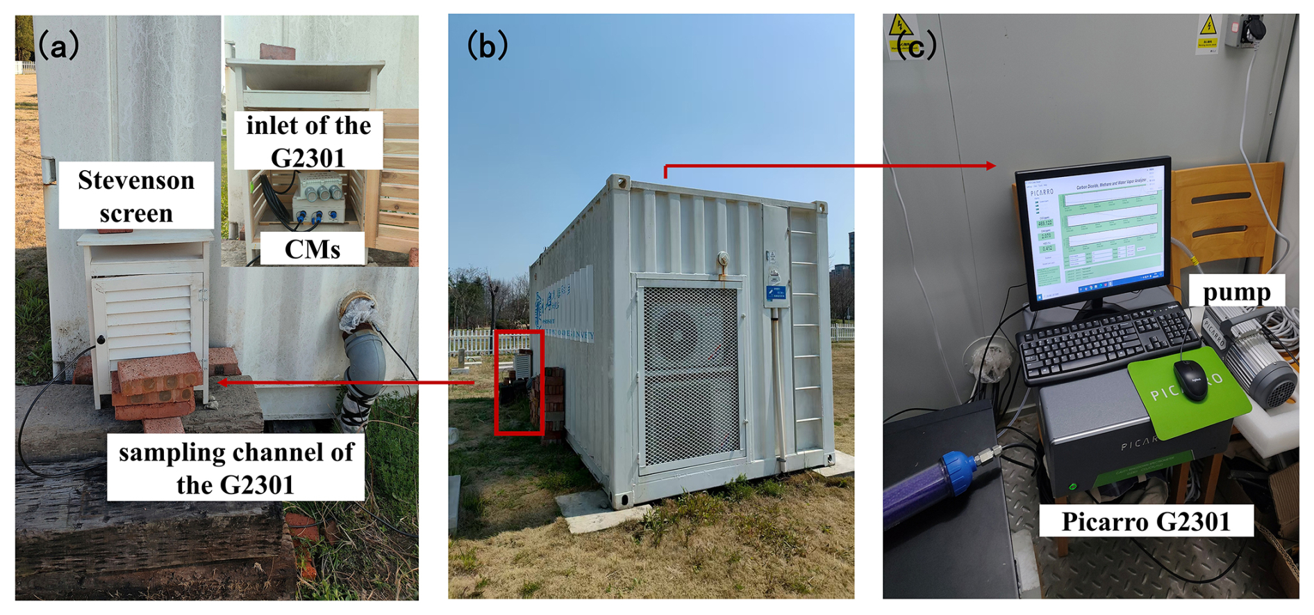
Figure 3 Land-based field observation experiments. (a) Configuration of CMs, Stevenson screen, and Picarro sampling channel. (b) Meteorological observation station, experimental cabin, and field deployment of CMs. (c) Field setup of the Picarro G2301.

To calibrate the CMs, it was first placed in the laboratory and a meteorological observation field within Jiangwan Campus of Fudan University, for side-by-side observations with a cavity ring-down spectrometer (Picarro G2301, Picarro Inc., Santa Clara, USA) (Fig. 3). The CMs equipped with Stevenson screen was placed outside the station building, while the sampling gas tube of Picarro was extended into the Stevenson screen through a duct connecting the station building to the outside environment, ensuring simultaneous observations with CMs. Following land-based field observations, the instrument was deployed for field observations at sea. The offshore field observation point is located in the coastal area of Dianbai District, Maoming City, Guangdong Province (21.44° N, 111.39° E) (Fig. 1a), belonging to northern shelf coastal section of the South China Sea nearshore areas feature port zones, shallow bays, and small islands (such as Dazhuzhou), while offshore lies the broad continental shelf and slope transition zone of the northern South China Sea. Integrated multi-source observations indicate that most of the South China Sea is a weak to moderate CO₂ source with seasonal variations (Zhai et al., 2013; Li et al., 2020; Chen et al., 2024; Zhang et al., 2024). The annual average flux in the northern continental slope region is approximately 0.46 $\mathrm{mol}{\mathrm{m}}^{-\mathrm{2}}{\mathrm{yr}}^{-\mathrm{1}}$, with higher values in the central and southern areas (about 1.37 $\mathrm{mol}{\mathrm{m}}^{-\mathrm{2}}{\mathrm{yr}}^{-\mathrm{1}}$) (Zhai et al., 2013). During summer, the coastal upwelling brings up subsurface water rich in dissolved inorganic carbon and low in temperature to the surface layer, typically tending to increase atmospheric CO₂ emissions. However, spatiotemporal variations in wind events, biological consumption, and estuarine runoff can cause significant short-term or inter seasonal reversals (Xu et al., 2013; Li et al., 2021). In summary, the northern South China Sea, where the observation point in this study are located, is generally characterized as a minor CO₂ source but exhibits strong spatiotemporal variability (Zhang et al., 2024).

2.2 CMs data correction method

The original signals had a sampling interval of 2 s and a background noise level of ± 30 ppm. The raw data from the CMs were filtered and resampled. After quality control, outliers deviating by more than 4σ from the mean were removed – this detection was implemented on the native 2 s resolution data within consecutive 1 min windows (30 raw data points per window) – and temporal averaging was applied to reduce the noise level. The 4σ threshold is applied to achieve a compromise between eliminating extreme outliers and retaining the inherent variability of the dataset (Cai et al., 2025). Allan variance, which quantifies the time-averaged stability of continuous measurements, was used to determine the optimal averaging interval that minimizes noise while preserving the integrity of the data signals (Martin et al., 2017). Langridge et al. (2008) indicated that the optimal averaging time for the Allan variance of the K30 sensor to reach its minimum is approximately 3 min, after which extending the averaging time step no longer significantly reduces the noise. Cai et al. (2025) evaluated the noise characteristics of the SenseAir K30 by continuously introducing standard gases. The results showed that at a measurement interval of 2 s, the noise level was 4 ppm, and 1–2 min showed 0.4–0.7 ppm noise level, and from 2 min to 1 h, the noise level decreased to approximately 0.2 ppm.Although the 3minute interval yields a marginally lower Allan variance, a 1 min averaging time was adopted in this study because the Allan variance is only slightly higher than at 3 min while allowing resolution of shorter-time scale atmospheric variability (Martin et al., 2017). This choice ensures sufficiently low noise (0.4–0.7 ppm) to resolve marine CO₂ dynamics while preserving higher-frequency variability associated with rapid coastal atmospheric and air–sea CO₂ exchanges that would be smoothed over with 3 min averaging, and supports detailed process analysis with the flexibility to aggregate to coarser scales as needed.

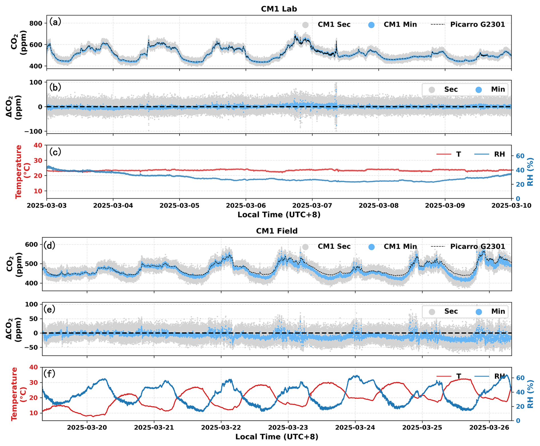
Figure 4 Time series of CM1 data during laboratory (a–c) and land-based field (d–f) observations. (a, d) CM1-measured CO₂ concentration at second-level resolution (grey dots) and minute-level resolution (blue dots), alongside Picarro-measured CO₂ concentration (black line). (b, e) Time series of CO₂ concentration difference (ΔCO₂=CM1-Picarro) at second-level (grey dots) and minute-level (blue dots) resolution. (c, f) Time series of ambient temperature (T, red line) and relative humidity (RH, blue line).

Using CM1 as an example, results from observations conducted by CMs and Picarro in laboratory and terrestrial field are presented in Fig. 4. After quality control and resampling of raw data, the standard deviation (SD) for the three CMs in laboratory tests improved from 13.05, 17.32, 18.28 to 4.68, 5.26, and 5.48 ppm, respectively. For field tests, the values improved from 15.14, 21.93, 17.06 to 9.33, 14.83, and 8.83 ppm, respectively (Figs. 4 and S1 and S2 in the Supplement). Data accuracy improved after minute averaging (Fig. 4a and d), but differences still exist compared to the reference instrument Picarro (ΔCO₂). A comparison between the laboratory and field results (Fig. 4a and d) shows that the CMs performed better under laboratory conditions. In the stable laboratory environment, ΔCO₂ exhibited no pronounced diurnal variation (Fig. 4b and e), fluctuating steadily around a constant value (system bias). By contrast, in the field, where atmospheric conditions naturally vary (Fig. 4f), the environmental parameters showed clear diurnal cycles, and ΔCO₂ also displayed diurnal oscillations. In addition, during the field deployment, ΔCO₂ exhibited a gradual downward “temporal trend” over the observation period (Fig. 4e), which is closely related to changing environmental conditions. Apart from the diurnal cycle, ambient temperature exhibited a marked upward trend over several consecutive days (Fig. 4f). As will be discussed in Sect. 3, the ΔCO₂ of CM1 is negatively correlated with temperature, indicating that rising temperatures lead to a decrease in ΔCO₂. Therefore, the observed downward trend in ΔCO₂ is physically consistent with the gradual rise in temperature, reflecting a temperature-driven response rather than inherent sensor instability. This indicates that the CMs are highly sensitive to environmental conditions, and their measurement accuracy is affected by both atmospheric variability and the CO₂ concentration baseline. Therefore, further calibration with respect to environmental parameters is required. The most used environmental correction method for NDIR sensors is multiple linear regression. This involves establishing empirical regression models using environmental parameters such as temperature, air pressure, and water vapor under laboratory or side-by-side observations with standard instrument (Martin et al., 2017; Han et al., 2024; Cai et al., 2025). In recent years, numerous studies have attempted to model environmental nonlinear effects using machine learning methods such as random forests, gradient boosting, or neural networks, achieving lower root mean square error (RMSE) than linear regression (Biagi et al., 2024; Dubey et al., 2024). However, these approaches still exhibit limitations in interpretability and transferability.

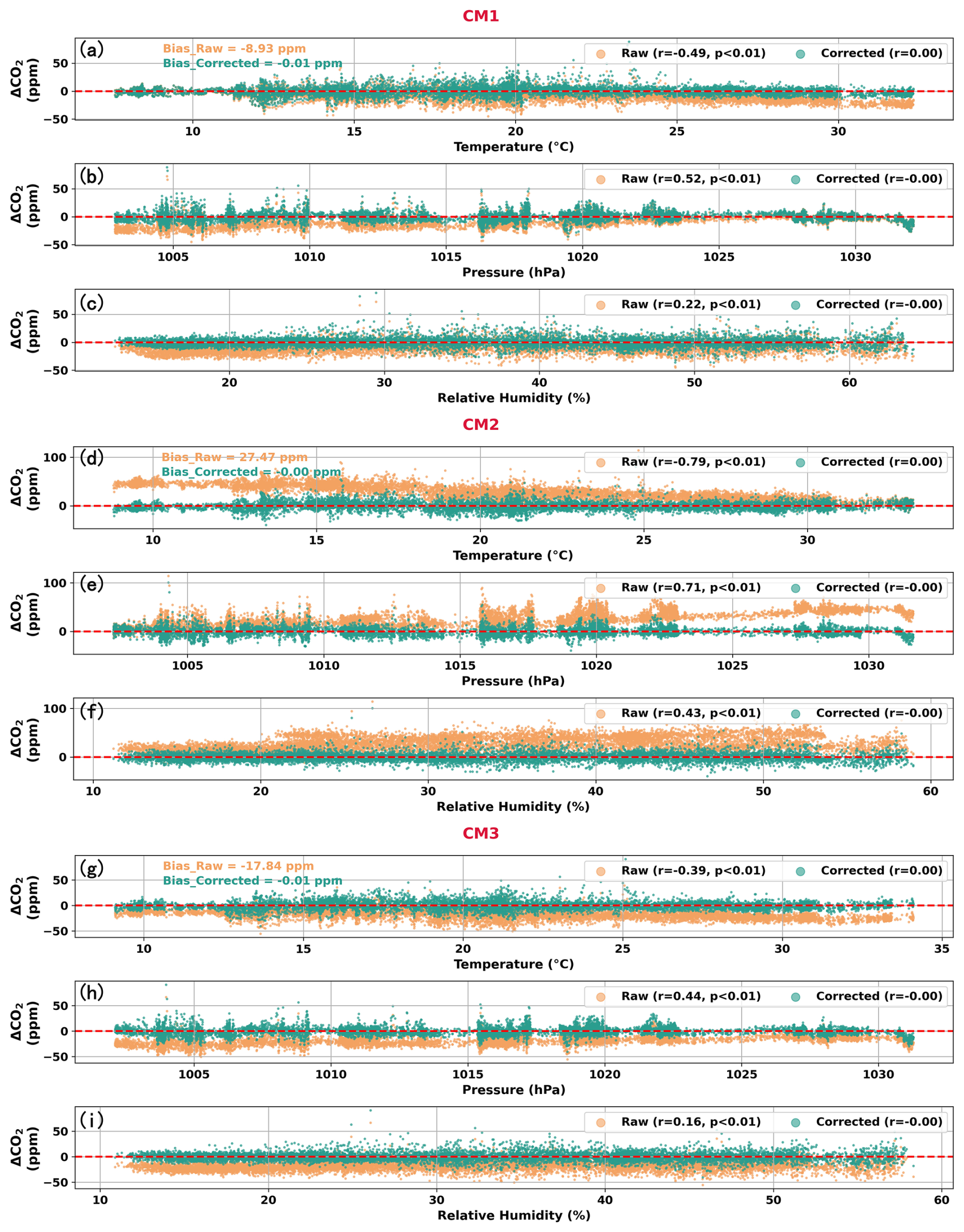
Figure 5 Variations of ΔCO₂ (ΔCO₂=CM-Picarro) for CM1 (a–c), CM2 (d–f), and CM3 (g–i) during land-based field observations, as functions of temperature (a, d, and g), atmospheric pressure (b, e, and h), and relative humidity (c, f, and i). Orange dots represent data before environmental correction, while green dots represent data after environmental correction.

The 1 min ΔCO₂ exhibits linear relationships with T, P, and RH, and this environment-related dependence differs among individual CMs (Fig. 5). Based on these characteristics, this study adopts a multiple linear regression approach for environmental calibration as Cai et al. (2025), where ΔCO₂ and the environmental parameters satisfy the following relationship:

$$\begin{array}{}\text{(1)}& {\displaystyle }\mathrm{\Delta }C=Y_{\text{CM}}-y_{\mathrm{0}}\text{(2)}& {\displaystyle }\begin{array}{rl}\mathrm{\Delta }C=& a_{\mathrm{0}}+f(a_{\mathrm{t}},T)+f(a_{\mathrm{p}},P)+f(a_{\text{RH}},\text{RH})\\ & +f(a_{\mathrm{c}},{\mathrm{CO}}_{\mathrm{2}})\end{array}\end{array}$$

Here, Y_CM represents the CMs measurements, and y₀ is the true atmospheric CO₂ concentration. The coefficients a_t, a_p, a_RH, and a_c are the correction parameters associated with T, P, RH, and the CO₂ concentration, respectively; including the CO₂ term in the calibration equation serves to eliminate the zero-point bias of the CMs. For each CM, the corresponding values of a_t, a_p, a_RH, and a_c are unique. a₀ is the baseline concentration correction parameter, calibrated using measurements from reference instruments at the observation site or from nearby atmospheric background stations. All these parameters can be determined through multiple linear regression using the Linear Regression function in Python. It should be specifically noted that temporal drift of the sensor was evaluated (Fig. S3 in the Supplement). Previous studies have incorporated linear time terms into calibration models to account for sensor aging and drift (Arzoumanian et al., 2019). In the present study, however, the apparent temporal trend in raw error is associated with the gradual increase in temperature during the measurement period. After correction, no consistent linear relationship was observed between sensor error and time. Therefore, a linear time term (t) was not included in the regression model. For long-term monitoring, periodic re-calibration every 3–6 months using stable atmospheric CO₂ observations from background reference sites (e.g., MLO) during quiescent atmospheric conditions will be required to address non-linear temporal drift.

The corrected data of CO₂ after environmental correction is:

$$\begin{array}{}\text{(3)}& \begin{array}{rl}{y}_{\text{corrected}}=& Y_{\text{CM}}-a_{\mathrm{0}}-f(a_{\mathrm{t}},T)-f(a_{\mathrm{p}},P)\\ & -f(a_{\text{RH}},\text{RH})-f(a_{\mathrm{c}},{\mathrm{CO}}_{\mathrm{2}})\end{array}\end{array}$$

When standard instrument (e.g., Picarro) co-located observations are available, these measurements shall be considered the true values for atmospheric CO₂ concentrations. The specific correction results will be described in Sect. 3. For marine observations, the baseline correction of CMs is performed using data from the Mauna Loa atmospheric background station in Hawaii, USA (Thoning et al., 2025), corresponding to periods where CMs observations are stable and close to background values. The specific method and results will be introduced in Sect. 4.

3 Environmental correction results for land-based field observations

Temperature variations affect the sensor's light source intensity, detector response, and absorption cross-section, leading to systematic drifts in output (Yasuda et al., 2012). Pressure influences gas density and infrared absorption line broadening, making corrections based on the equation of state or sensor sensitivity particularly important in regions with strong pressure fluctuations (Chen et al., 2010; Curcoll et al., 2022). Water vapor exerts the most complex effects on NDIR sensors: it not only dilutes CO₂ mole fractions in moist air relative to dry air but also causes spectral line broadening within the CO₂ absorption band, introducing biases (Chen et al., 2010; Dubey et al., 2024). Accordingly, the multivariate linear calibration of CMs focuses on 3 key environmental factors – T, P, and RH. Figure 5 shows the variations of ΔCO₂ between the three CMs and the collocated Picarro measurements as a function of environmental parameters (T, P, and RH) during the land-based field observations, where the orange and green colors correspond to the data before and after environmental correction, respectively. Figure 6 presents the linear relationships between the CMs and the Picarro, along with the histograms of ΔCO₂.

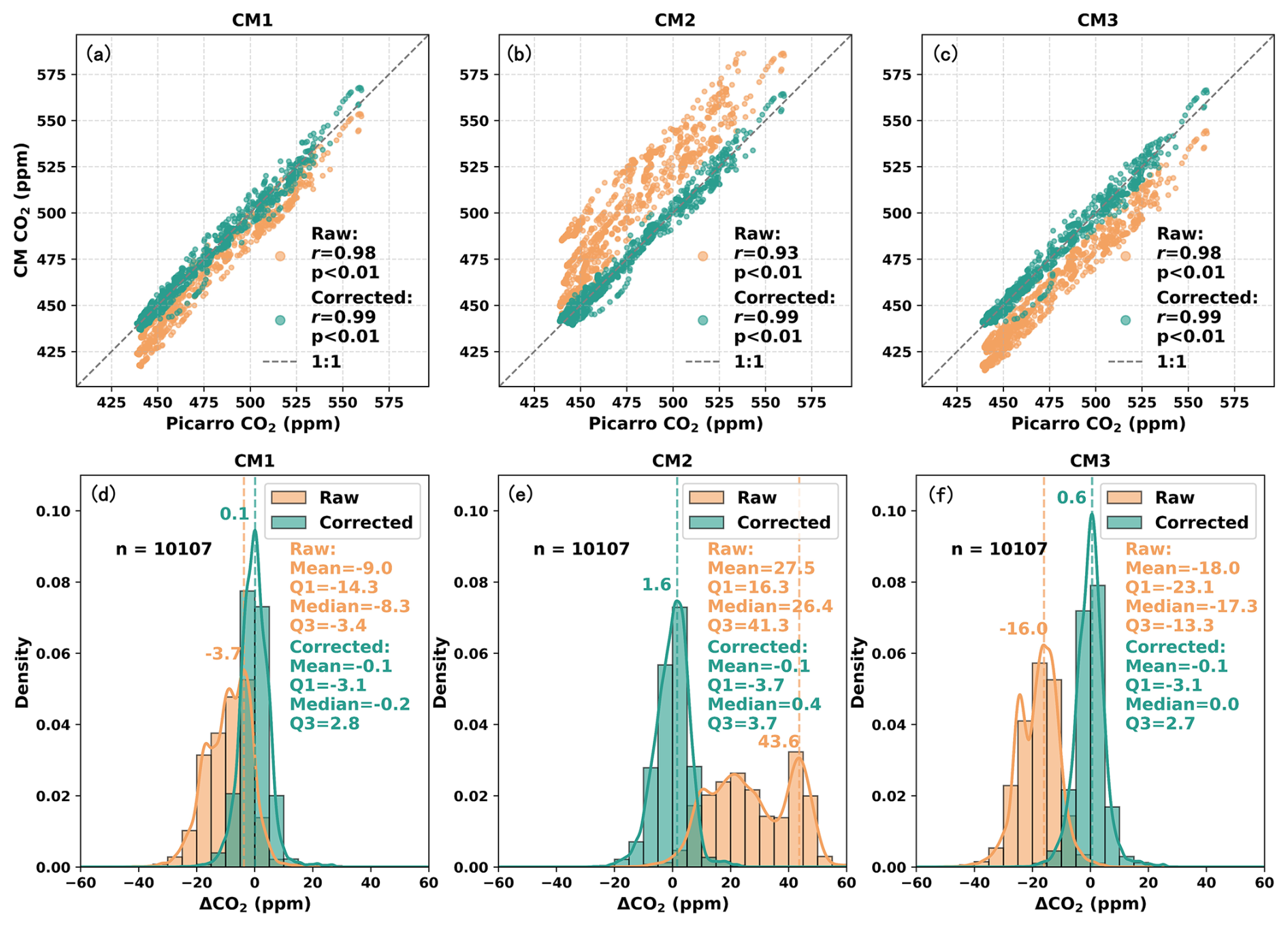
Figure 6 Direct comparison of hourly moving averages of CO₂ concentrations among CM1, CM2, CM3 and Picarro during land-based field observations (a–c), and histograms of ΔCO₂ distributions (d–f) (ΔCO₂=CM-Picarro, where CM corresponds to CM1, CM2, and CM3, respectively). Orange dots and bars represent data before environmental correction, while green dots and bars represent data after environmental correction.

Prior to correction, the ΔCO₂ of all three CMs exhibited linear relationships with environmental parameters (Fig. 5): negative correlation with T, and positive correlation with P and RH. Among these, CM2 demonstrated the most pronounced correlations. The correlation coefficients (r) between ΔCO₂ and T, P, and RH were −0.79, 0.71, and 0.43, respectively, while the r values for CM1 and CM3 were −0.49, 0.52, 0.22, and −0.39, 0.44, 0.16, respectively, all significant at the 0.01 level (p < 0.01). After correction, the systematic drift of ΔCO₂ across the three CMs due to environmental parameters was successfully eliminated. The corresponding r values were all 0, indicating no significant correlations, with ΔCO₂ fluctuating around the zero line. Beyond environmental factors, the multiple linear regression also incorporated the true CO₂ concentration in the atmosphere, represented by Picarro co-located measurements in field observations. The values of the first three CMs before correction all exhibit zero bias relative to the true values (the fit between CO₂ observations and true values includes intercepts) (Fig. 6a–c), with respective r values of 0.98, 0.93, and 0.98, all significant at the 0.01 level (p < 0.01). After correction, the correlations all improved to 0.99 (p < 0.01), and data points largely converged on either side of the 1:1 line. The bias between CMs and Picarro shifted from −3.7, +43.6, and −16 to +0.1, +1.6, and +0.6 ppm, respectively, shifting from significantly biased to essentially unbiased (Fig. 6d–f). The results above suggest that all three CMs are influenced by environmental variables, but to markedly different extents. Whether for CM2, which inherently exhibits substantial systematic errors, or CM1, which shows minimal data offset prior to correction, our environmental correction method significantly enhances observational accuracy, improves data quality, and demonstrates good universality.

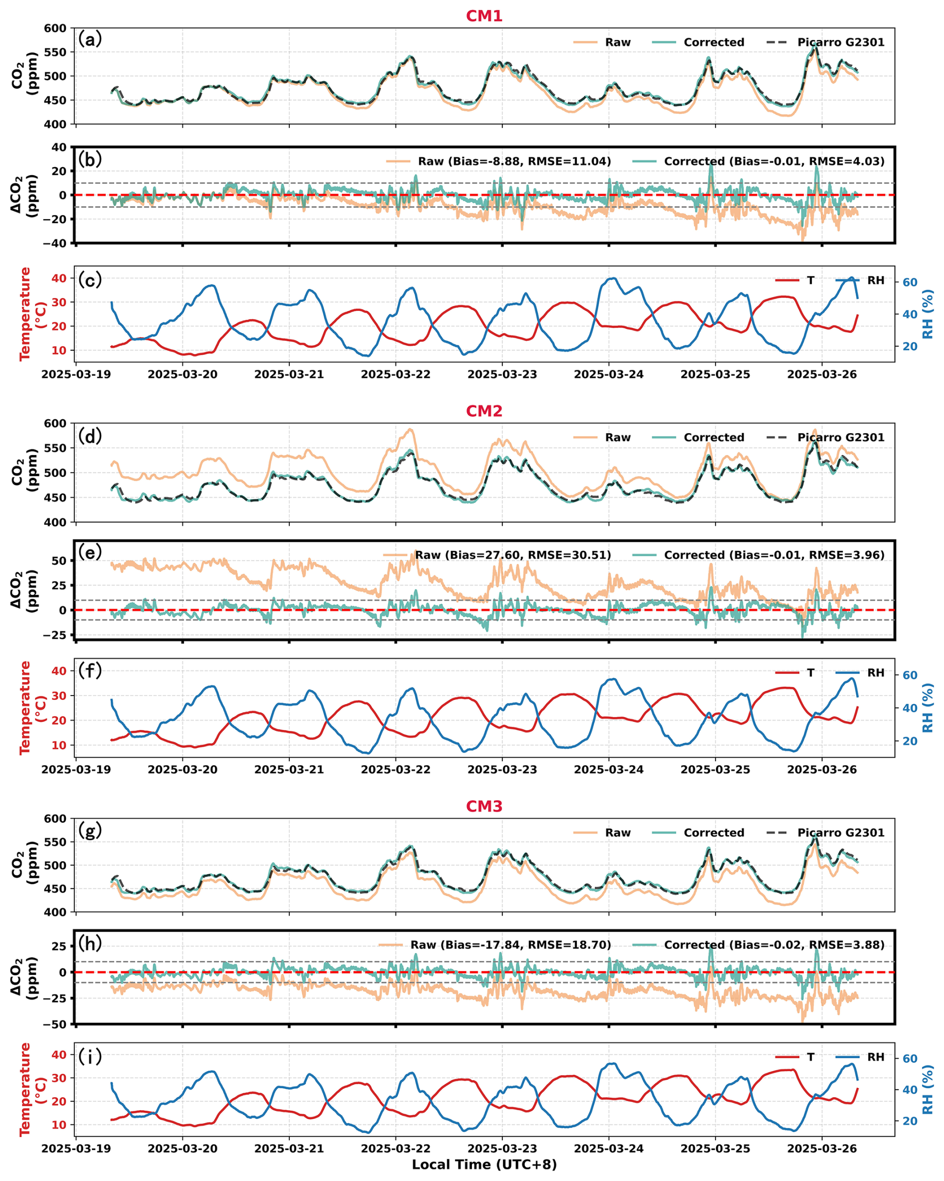
Figure 7 Hourly moving average time series of CM1 (a–c), CM2 (d–f), and CM3 (g–i) during land-based field observations: CO₂ concentration of CMs before environmental correction (orange line), after environmental correction (green line), and CO₂ concentration from Picarro (black dashed line) (a, d, and g); ΔCO₂ (ΔCO₂=CM-Picarro) of CMs before and after calibration (b, e, and h); Ambient temperature (T, red line) and relative humidity (RH, blue line) (c, f, and i).

Environmental correction effectively reduced the offset values between CMs and Picarro (Fig. 7). Before correction, CMs captured CO₂ concentration trends like Picarro but exhibited significant deviations. For the best performing CM1, this deviation was particularly noticeable at low CO₂ concentrations, while CM2 and CM3 showed overall high and low biases, respectively. The ΔCO₂ of CMs exhibited a certain “downward” drift trend over the one-week observation period, CM1 and CM3 moved from zero toward negative values, while CM2 shifted from a relatively high positive value around 50 ppm toward zero. The calibrated results showed high consistency with Picarro, with the RMSE decreasing from 11.04, 30.51, and 18.70 to 4.03, 3.96, and 3.88 ppm, respectively. The correction effectively eliminated the linear drift trend of ΔCO₂ over time, stabilizing it to fluctuate around the zero line. During the land-based field observations in Shanghai in early spring, the atmospheric temperature and humidity exhibited pronounced diurnal variations, fluctuating between 5–30 °C and 10 %–60 %, respectively. The average RMSE of corrected CMs was 3.64 ppm, which is sufficient to capture terrestrial CO₂ variations (400–600 ppm), even during periods of significant CO₂ fluctuations with pronounced peaks and troughs, such as cases on 22–23 March and 25–26 March, where the environmental correction method performed well.

4 Marine observation results

Based on the instrument deployment and marine environment described in Sect. 2, and the environmental correction method validated through land-based field observations in Sect. 3, the CMs-equipped air–sea interface buoy observation platform commenced operation in May 2025 in the northern South China Sea off the coast of Dianbai District, Guangdong Province. Following signal debugging and regular equipment maintenance, observational data were obtained over 3 months from 28 May to 28 August. The hourly moving-averaged time series of CO₂ concentration, T, and RH from the 3 CMs are shown in Fig. 8. During environmental calibration, measurements are first corrected using the environmental coefficients a_t, a_p, a_RH, and a_c obtained from land-based calibration; baseline correction is then applied by updating a₀ with reference CO₂ concentrations from the marine atmospheric boundary layer. Over the open ocean, strong horizontal atmospheric mixing results in small zonal variations in marine boundary layer CO₂ concentrations, indicating high zonal uniformity at similar latitudes (Bakwin et al., 2004; Palter et al., 2023). Given the strong real-time nature of this study's observations and the limited availability of co-located and near-surface observation resources, CO₂ observation data from the Mauna Loa atmospheric background station in Hawaii, USA (MLO, 19.54° N, 155.58° W) – located at a latitude similar to the observation site – served as the reference value. The CO₂ datasets were obtained from the NOAA Global Monitoring Laboratory (GML) (https://gml.noaa.gov/ccgg/trends/data.html, last access: 23 April 2026; Lan and Keeling, 2025). The relatively stable period (17–24 June) of CMs concentrations during the observation was regarded as the atmospheric background state. Both values were substituted into a multiple linear regression calculation to obtain a₀. After environmental correction, the RMSE of the CMs significantly decreased from 9.27, 52.39, and 11.24 to 1.57, 1.86, and 1.52 ppm, respectively (Figs. 8a and S4–S6 in the Supplement). The lower RMSE during the marine test can be partly explained by the substantially lower ambient CO₂ variability over the ocean, as reflected by the smaller standard deviation of the MLO reference data (1.81 ppm) compared to that of the Picarro in-situ measurements at the land site (29.29 ppm).

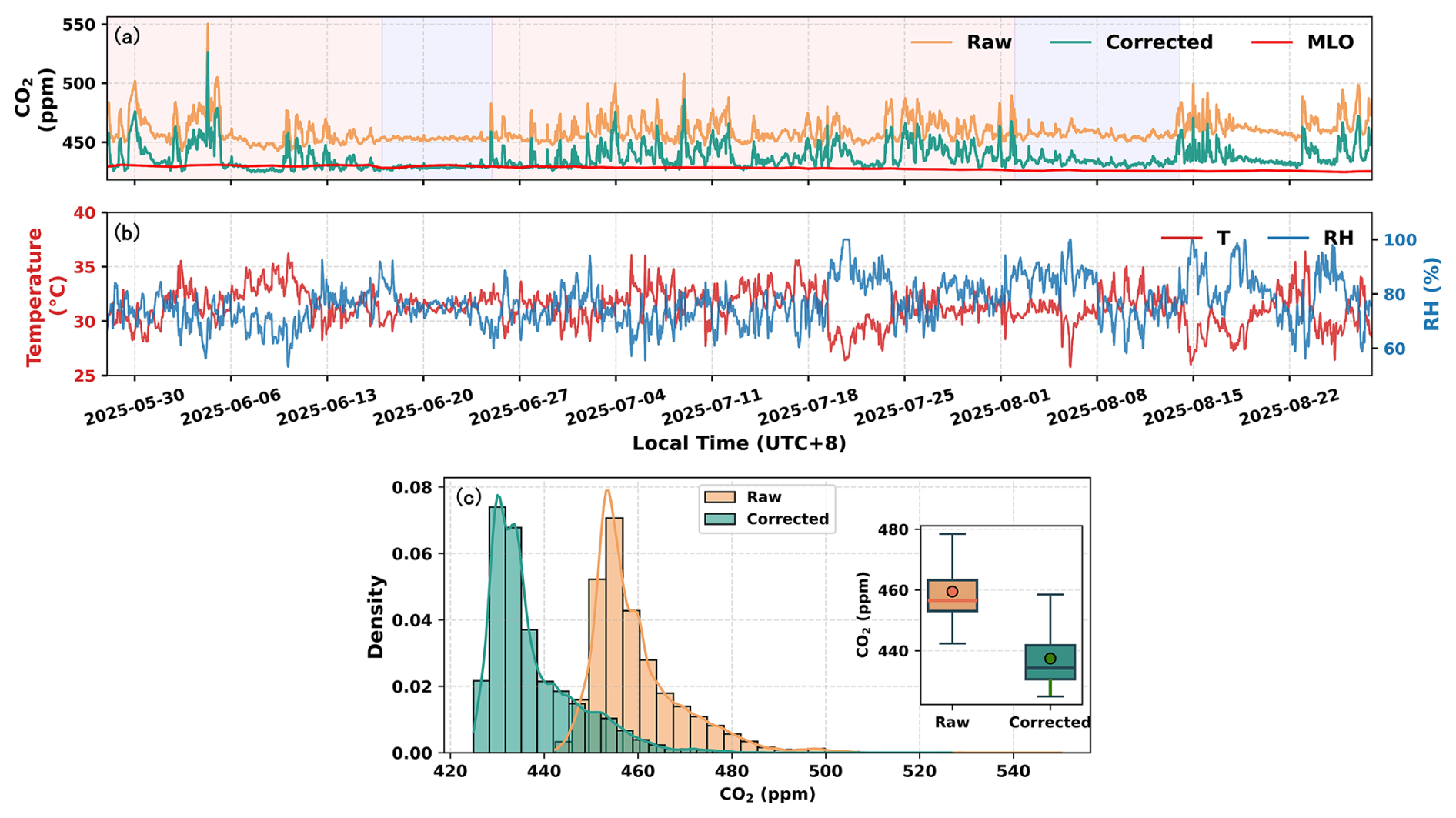
Figure 8 Offshore buoy observation results of CMs. (a) Hourly moving average time series of CO₂ concentrations from CMs before correction (orange line) and after correction (green line), together with daily mean CO₂ series from Mauna Loa Observatory (MLO, red line). The light red and light blue shaded backgrounds correspond to CO₂ fluctuation periods and stable periods, respectively. (b) Time series of ambient temperature (T, red line) and relative humidity (RH, blue line). (c) Histograms and boxplots showing the distributions of CO₂ concentrations before (orange bars) and after correction (green bars).

During the 3 month marine observations, the atmosphere at the observation site exhibited high temperatures and humidity, with temperatures ranging from 25 to 37.5 °C and humidity levels between 50 % and 100 % (Fig. 8b). Both showed pronounced diurnal and weekly variations. The mean CMs values before and after correction were 459.48 and 436.94 ppm, with medians of 456.53 and 433.75 ppm, respectively (Fig. 8c). The means consistently exceeded the medians, and the ranges surpassed 100 ppm in both cases, which indicates many signal peaks in CO₂ during the observation, and the observation site is susceptible to terrestrial anthropogenic CO₂ emissions. After correction, the overall concentration was approximately 22 ppm lower than the original values, consistent with the CO₂ range at the atmospheric background station MLO (mean 429.32 ppm). The correction eliminated systematic overestimation, bringing the results closer to background concentrations.

The SD of the raw data is 9.79 ppm, showing a slight difference from the corrected value of 9.62 ppm. The first quartile (Q1) changed from 453.08 to 430.10 ppm, and the third quartile (Q3) changed from 463.29 to 441.32 ppm, with an inter-quartile range (IQR) of 10.21 ppm, slightly below the corrected value of 11.22 ppm. These indicate that the correction process reduced the overall CO₂ concentrations but did not significantly decrease data variability. In fact, the distribution of the middle 50 % of data points became wider. Whether considering the extreme fluctuation range (extreme value difference) influenced by anthropogenic land effects, the typical fluctuation range IQR after removing most extreme signals, or the average fluctuation amplitude SD of overall concentrations, the accuracy of CMs corrected data is sufficiently to capture the corresponding signals.

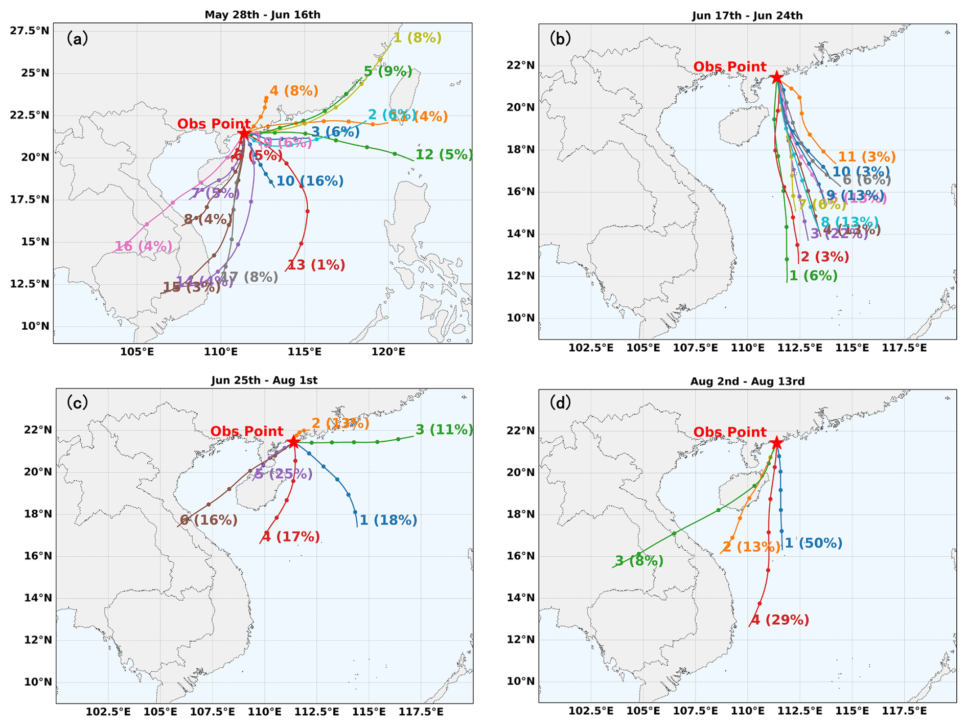
Figure 9 Clustered results of 36 h backward trajectories from Hybrid Single-Particle Lagrangian Integrated Trajectory (HYSPLIT) model analyses at the offshore observation site during four time periods of buoy observations. Each trajectory is labeled with its cluster number and proportion, and markers on the trajectories indicate 6 h intervals. (a) 28 May–16 June, (b) 17–24 June, (c) 25 June–1 August, (d) 2–13 August. (a) and (c) correspond to CO₂ concentration fluctuation periods, while (b) and (d) correspond to CO₂ concentration stable periods.

During the 3 month observation period, CO₂ at the monitoring site exhibited short-term fluctuation peaks as well as periods of stable concentrations, both of which can be analyzed and interpreted from the perspective of atmospheric transport. Using the NOAA Hybrid Single-Particle Lagrangian Integrated Trajectory (HYSPLIT) model, 36 h backward trajectories were calculated for the observation point to identify the primary transport pathways influencing the air mass sources at the location (Cohen et al., 2015). The trajectory origin is set at the observation point, with a time resolution of 6 h. Meteorological driving data were from the Global Data Assimilation System (GDAS1, 1° × 1°) reanalysis data provided by NOAA (Rolph et al., 2017). After obtaining a series of backward trajectories, the HYSPLIT clustering module was employed to classify the trajectories. This approach mitigates the impact of uncertainty inherent in individual trajectories and extracts key transport pathway characteristics, providing a basis for subsequent analysis of the relationship between air mass transport and observational results (Cohen et al., 2015). The entire period of marine observations was divided into four segments for clustering. The periods from 28 May to 16 June (Fig. 9a) and 25 June to 1 August (Fig. 9c) constituted CO₂ fluctuation phases (the background is light red in Fig. 8a), with many concentration peaks occurring during these periods. The periods from 17 to 24 June (Fig. 9b) and 2 to 13 August (Fig. 9d) constituted CO₂ stable phases (the background is light blue in Fig. 8a). During these phases, CO₂ concentrations fluctuated minimally and approached the background levels of the marine boundary layer. It is particularly noteworthy that during the two-week period from 14 to 28 August (the background is white in Fig. 8a), CO₂ exhibited alternating patterns of relatively dense peaks and sustained background concentration levels, with each state lasting no more than five days. The limited number of trajectories obtained from segmented analysis makes it inconvenient for cluster analysis.

The trajectory clustering results (Fig. 9) indicate that the atmospheric transport pathways corresponding to concentration fluctuation periods are relatively complex, significantly influenced by air masses transported from land. Trajectories from 28 May to 16 June were classified into 17 categories, with 40 % originating from land and 60 % from the ocean. The most typical inland air mass, represented by Trajectory 4, was transported from northern Guangdong all the way to western Guangdong. Trajectory 12, although originating from the sea, reached the observation point via the western coast of Guangdong within the first 6 h of the observation period. From 25 June to 1 August, trajectories ending over land accounted for 54 %, while those ending over the ocean accounted for 46 %. Trajectory 2, corresponding to short-range inland transport, accounted for 13 %. The clustering results indicate that local urban emissions from land areas significantly contributed to CO₂ concentrations at the observation point, effectively explaining the observed large fluctuations and multiple peaks during the corresponding period. Correspondingly, air masses at observation point during concentration stable periods were predominantly transported from clean marine atmospheres. The trajectories from 17 to 24 June were clustered into 11 groups, all originating from the South China Sea. Consequently, the observed CO₂ concentrations during this period remained near background levels, which can be considered the CO₂ concentration level in clean air without anthropogenic pollution. This also demonstrates that using CO₂ observations from this period combined with MLO atmospheric background concentrations for baseline correction of CMs is reasonable. Trajectories from 2 to 13 August were categorized into 4 types, with 92 % originating from marine sources and 8 % from land sources. Consequently, although CO₂ concentrations at observation point during this period were slightly elevated above background values, they remained generally stable.

By comparing the corrected CMs data during the concentration stable periods (including 19 complete days) with the diurnal variations in CO₂ concentration during the summer of 2024 (June to August) at the MLO station (Fig. 10), we can further understand how CMs captures the diurnal variation of oceanic boundary layer CO₂. Hourly CO₂ mole fractions at MLO were obtained from NOAA GML (https://gml.noaa.gov/data/dataset.php?item=mlo-co2-observatory-hourly, last access: 23 April 2026; Thoning et al., 2025). Both CMs and MLO exhibit daily variations in background CO₂ concentrations characterized by lower daytime values and higher nighttime values. This pattern likely stems from the primary influence of air–sea CO₂ fluxes and atmospheric convective transport on oceanic CO₂ concentrations (Lv et al., 2015). During the day, solar radiation heats the Earth's surface, which enhances photosynthesis in marine ecosystems and promotes the uptake of atmospheric CO₂. As atmospheric temperatures rise, enhanced turbulent activity thickens the atmospheric boundary layer, diluting CO₂ through vertical atmospheric mixing and reducing its concentration. At night, photosynthesis ceases in regional marine ecosystems, leaving only respiration. The sea surface cools, and weakened turbulent mixing restricts vertical air exchange.CO₂ struggles to diffuse into the upper layers, accumulating in the near-surface layer and increasing in concentration. The daily amplitude of CO₂ at MLO station during summer is approximately 2 ppm, while CMs is 3 ppm. This indicates that the environmentally calibrated CMs is sufficiently sensitive to capture the daily variation signal of CO₂ in clean background air unaffected by terrestrial anthropogenic emissions, demonstrating its potential for observing atmospheric CO₂ concentrations in open ocean environments. The daily amplitude of CO₂ at MLO Station during summer is approximately 2 ppm, while CMs is 3 ppm. This indicates that the environmentally calibrated CMs is sufficiently sensitive to capture the daily variation signal of CO₂ in clean background air unaffected by terrestrial anthropogenic emissions, demonstrating its potential for observing atmospheric CO₂ concentrations in open ocean environments.

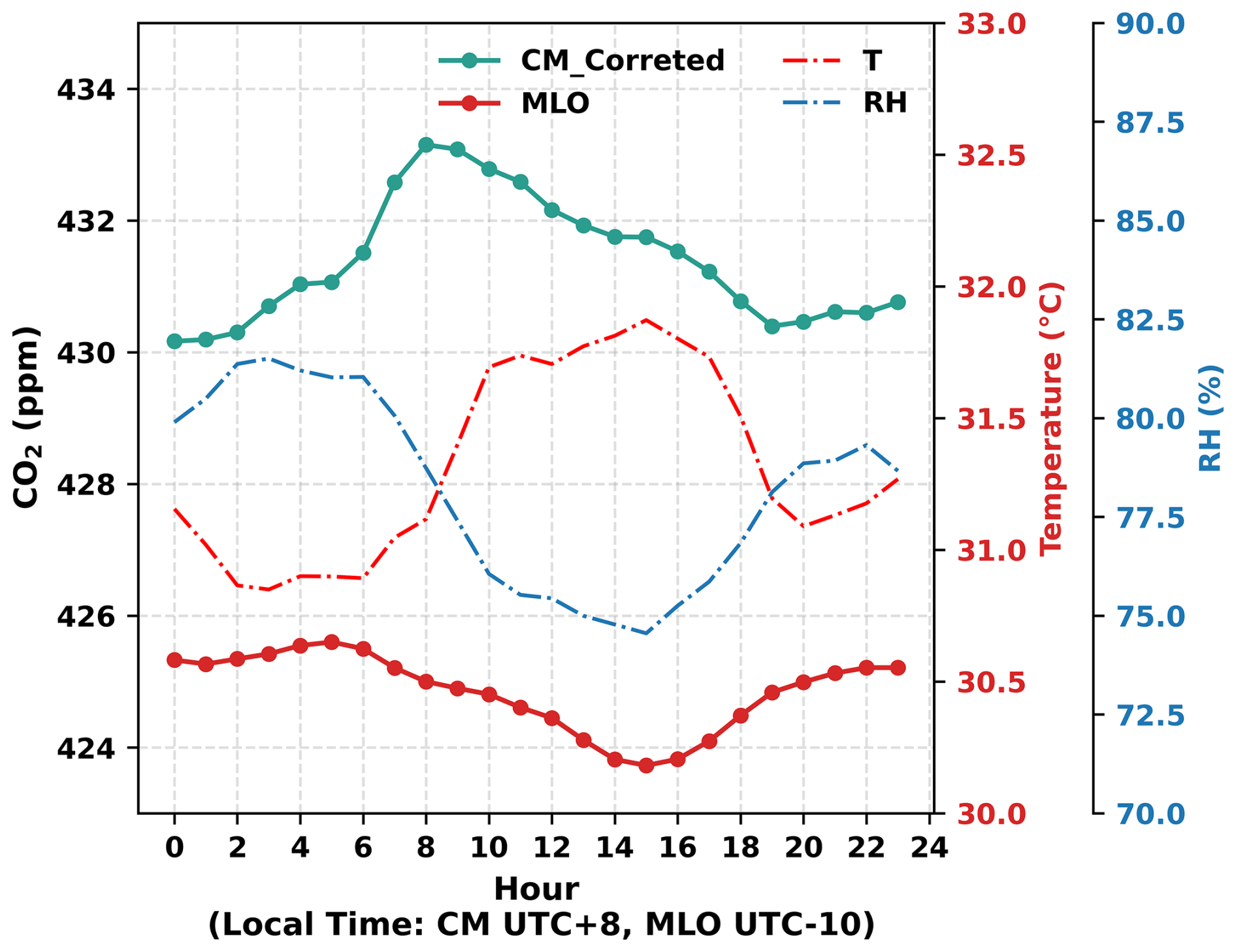
Figure 10 Diurnal variations of CO₂ concentrations from CMs (environmentally corrected, green line) during stable concentration periods and from Mauna Loa Observatory (MLO, June–August 2024, red line), along with corresponding temperature (T, red dash line) and relative humidity (RH, blue dash line) variations.

Observations of the CMs show that the daily maximum and minimum values of CO₂ exhibit a 3 h lag compared to the MLO station, which may be attributed to differences in the surrounding environments of the two sites. The MLO station is situated on high altitude land, exhibiting a typical mountainous diurnal variation in CO₂ concentration. Mountainous terrain induces strong upslope and downslope airflows, leading to earlier atmospheric mixing. During the day, upslope flow and mixing intensify (NOAA GML, 2024a), resulting in the lowest concentrations around 4 p.m. when vertical mixing is strongest. At night, the mountain air becomes isolated from the free atmosphere, with downslope flows carrying high CO₂ air (NOAA GML, 2024a), reaching peak concentrations around 6 a.m. The observation site in this study is over an ocean surface, which possesses high thermal capacity, exhibits small diurnal temperature variations, and experiences delayed turbulence enhancement and boundary layer development (Nemoto et al., 2009). Consequently, the nocturnal accumulation of CO₂ persists until 8 a.m., several hours after sunrise. Daytime sea breezes and mixing intensify later, with the lowest CO₂ values occurring around 7 p.m. The average CO₂ concentrations at MLO and CMs were 424.85 and 431.38 ppm, respectively, differing by approximately 6.5 ppm. This discrepancy may be due to the fact that the comparison uses 2024 data. According to the NOAA, the annual growth rates of CO₂ concentrations for MLO 2023 and 2024 were 3.36 and 3.33 ppm yr⁻¹ (NOAA GML, 2024b). Furthermore, even after filtering out short term terrestrial sources, the East Asian monsoon transport can still cause regional increases in atmospheric CO₂. This monsoon-driven transport represents mesoscale or large-scale processes, not local pollution peaks, and thus systematic differences between CO₂ concentrations and MLO can still be observed during stable periods (Fang et al., 2014; Lin et al., 2018).

5 Post-deployment laboratory validation

To evaluate long-term sensor stability, post-deployment laboratory calibrations were performed against the Picarro reference in March 2026, approximately 9 months after the initial June 2025 calibration. The results are summarized in Table 1.

Table 1 Post-deployment laboratory validation results (Units: ppm).

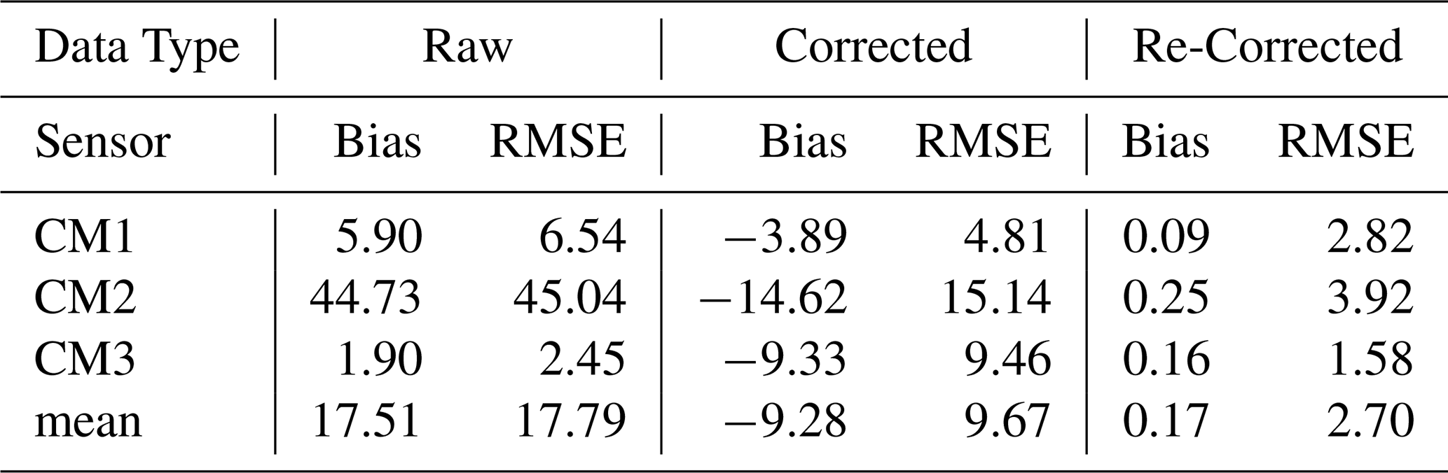
After marine deployment, noticeable sensor temporal drift is evident in the Corrected data (mean bias: −9.28 ppm, mean RMSE: 9.67 ppm). Performance varied among sensors; CM3 showed reduced accuracy under the original correction compared to its raw data, likely due to individual sensor variability over time. Crucially, sensor sensitivities to temperature, humidity, and pressure remained consistent throughout the deployment. Re-correction by updating the baseline parameter a₀? effectively compensates for this temporal drift, reducing the mean bias to 0.17 ppm and mean RMSE to 2.70 ppm. These results confirm that the environmental correction approach remains reliable for short-term deployments, while periodic re-calibration is essential for maintaining measurement accuracy in long-term marine observations.

6 Conclusions

We successfully established a sea–air interface buoy platform along the coast of Maoming, Guangdong Province, employing low-cost sensors to observe marine CO₂ concentrations in the nearshore region of the northern South China Sea. Environmental correction methods effectively eliminated the impact of environmental factors such as temperature, pressure, and humidity fluctuations on CO₂ measurements while correcting for zero bias. With land-based Picarro G2301 co-located observations for comparison, CO₂ accuracy improved from 8.03 to 3.64 ppm (corresponds to the 1 h moving average of minute-by-minute data). Over ocean, baseline correction using MLO atmospheric background station data improved accuracy from 24.26 to 1.59 ppm, meeting the precision requirements for capturing marine CO₂ concentration signals (e.g., 420–480 ppm in this research). Systematic errors were eliminated, ensuring observed overall concentration levels align with MLO background stations, thereby meeting CO₂ concentration levels in the marine boundary layer. The temporal variations in CO₂ observed by the CMs, including both fluctuating and steady-state phases, can be explained by the long-range atmospheric transport simulated by HYSPLIT. Moreover, the CMs successfully captured the diurnal variations of background CO₂ in the marine atmospheric boundary layer, with an amplitude of approximately 3 ppm.

In summary, this study proposes an environmental correction method for calibrating low-cost sensors, demonstrating its reliability and scientific validity. It has successfully facilitated the application of low-cost sensors aboard buoys for observing marine atmospheric CO₂ concentrations, providing valuable experience for field deployment of marine atmospheric CO₂ monitoring. To our knowledge, this marks the first application of this method, holding significant importance for acquiring CO₂ concentration data in under-observed marine regions. This approach significantly reduces the cost of observing CO₂ in the ocean, opening new possibilities for achieving the goal of substantially increasing observation data. At the same time, high-precision instruments demand stringent environmental conditions. When deployed on buoy platforms in the harsh field observation environment of the ocean, with its powerful winds and waves, maintenance becomes extremely difficult. Low-cost sensors, however, overcome these technical challenges to a large extent.

This study represents the first trial in deploying low-cost sensors aboard buoys to monitor marine CO₂ concentrations. The buoy platform equipped with CMs has withstood several typhoon events, demonstrating excellent watertightness, mechanical robustness, and stability under wave conditions. During deployment, the sensors maintained nearly 100 % operational uptime. Post-recovery inspection revealed only minor corrosion on external metallic components, while internal sensor modules remained intact and free of corrosion, further confirming their robustness and good mechanical strength in the harsh marine environment. The successful detection of daily variations in the CO₂ stable periods further demonstrates the method's potential for deployment in open ocean observations. To achieve the goal of significantly increasing the number of marine observations, low-cost sensors must be deployed on small drifting buoys in the following studies. The current short-term deployment does not allow for full assessment of long-term sensor drift, which will require correction in extended observations. Long-term operation of NDIR sensors is expected to introduce non-linear temporal drift associated with light source aging and detector degradation. Since such drift exhibits no consistent linear relationship with time, a linear correction coefficient was not adopted in this study. Instead, periodic re-calibration every 3–6 months using stable background CO₂ observations under quiescent atmospheric conditions is recommended for future long-term deployments. While the current short-term deployment confirms satisfactory real-world performance, a comprehensive assessment of long-term operational durability and lifespan requires extended multi-month to multi-year deployments, which will be conducted in future work with periodic recalibration and intercomparison. Future work will also aim at long-term buoy deployments to capture seasonal variability and further validate sensor performance under varying environmental conditions. In the future, if large-scale deployment of buoys for observation can be realized to obtain extensive regional oceanic CO₂ observational data, these data could be utilized for “top-down” atmospheric inversions. This would provide new perspectives and methodologies for estimating air–sea CO₂ fluxes, representing a groundbreaking endeavor. It holds significant importance for accurately estimating oceanic carbon sinks and quantifying the dynamics of the carbon cycle.