Evaluating machine learning model performance in a two-step colocation process for TVOC and BTEX sensor calibration

Calibration of low-cost air quality sensors (LCSs) for total volatile organic compound (TVOC) and benzene, toluene, ethylbenzene, and xylenes (BTEX) quantification remains challenging due to the sensors' cross-sensitivity to temperature and humidity and their tendency to drift over time. In this study, we aimed to improve TVOC and BTEX metal oxide (Figaro TGS 2600, 2602, 2611) sensor calibration using a two-step colocation strategy. A two-step colocation places one LCS (the secondary standard) with a reference monitor while others operate in the field, then briefly colocates the field sensors with the secondary standard to address inter-sensor variability and drift. This strategy made it possible to develop the calibration model under environmental conditions closely matching those of the field, which is essential for model transferability from colocation to field conditions. In addition to TVOC and BTEX, we applied the two-step colocation process to NO₂ electrochemical (Alphasense B-4) sensors to demonstrate the broader applicability of our approach beyond TVOC and BTEX quantification.

Next, we compared the performance of multiple machine learning models, including ridge, lasso, random forest, gradient boosting, extreme gradient boosting, support vector regression, and linear regression, to investigate the optimal model choice for calibration. We found that no single model performed best across all pollutants. For example, gradient boosting excelled at capturing peak TVOC concentrations, while linear regression performed best for BTEX. Conversely, linear regression was the worst-performing model for NO₂. Overall, the models showed satisfactory RMSE around 40–50 ppb for TVOC, 1.25–1.75 ppb for BTEX, and 4–6 ppb for NO₂. However, all models also overestimated baseline concentrations and underestimated peaks. The severity of this bias depended on the reference concentration distribution, with the most severe peak underestimation occurring in the more heavily skewed TVOC and BTEX data. The systematic bias at baseline and peak concentrations was not evident in the overall mean bias error, which was near zero for all pollutants. This result underscores the need to evaluate model performance across the entire concentration distribution. Finally, we found that calibration performance was sensitive to the choice of training and testing data split. Future research could seek to optimize the training and testing split to ensure robust model transferability to field data.

1 Introduction

Low-cost sensors (LCSs) are an increasingly popular tool used by community groups, scientific researchers, and local governments to document air quality impacts at spatial and temporal scales finer than are possible with regulatory or reference-grade monitoring (Fanti et al., 2021; Clements et al., 2017; Commodore et al., 2017; Okorn and Iraci, 2024). Despite their increasing usage, LCSs face limitations due to their reduced accuracy compared to reference-grade monitoring methods (Karagulian et al., 2019; Castell et al., 2017; Clements et al., 2017). To improve accuracy, LCSs are often calibrated via colocation with a reference instrument, which corrects sensor drift and cross-sensitivity to temperature, humidity, and non-target pollutants (Liang, 2021; Karagulian et al., 2019; Liu et al., 2020).

In a colocation, sensors are placed next to a reference-grade monitor for a set period. The sensor signal is then calibrated to the reference-grade concentration time series via a linear regression or machine learning calibration model (Liang, 2021; Okorn and Iraci, 2024). For certain pollutants, such as ozone and PM_2.5, this process can significantly improve the accuracy of LCSs (Barkjohn et al., 2021; Masiol et al., 2018). However, calibrating LCSs for other pollutants, especially volatile organic compounds (VOCs), has had more limited success (Clements et al., 2017; Collier-Oxandale et al., 2019), leading some users to interpret low-cost VOC data only qualitatively (Frischmon et al., 2025a; Raheja et al., 2022).

VOCs are a broad class of chemicals that originate from both natural sources, such as wildfires and vegetation, and anthropogenic sources, such as industrial solvents, consumer products, and fossil fuel extraction, refining, and combustion. VOCs impact respiratory and cardiovascular health and can cause secondary health impacts by contributing to the formation of secondary organic aerosols and tropospheric ozone (Kampa and Castanas, 2008; Haagen-Smit et al., 1953; Laaksonen et al., 2008). Benzene, toluene, ethylbenzene, and xylenes, or BTEX, are a subset of VOCs that are especially relevant to human health due to their carcinogenicity (Kampa and Castanas, 2008). Total VOCs (TVOCs) and subsets like BTEX are challenging to quantify using LCSs in part because of their relatively low ambient concentrations (Spinelle et al., 2017b). Additionally, the chemical makeup of TVOCs can include many different species to which LCSs exhibit varying sensitivities. Low-cost TVOC and BTEX sensors can also show greater sensitivity to temperature and humidity than to VOC species, and they exhibit drift over long-term use (Lewis et al., 2016; Collier-Oxandale et al., 2019). Given these challenges, researchers have had the greatest success in calibrating these sensors for indoor use only, where concentrations tend to be higher and temperature and humidity can be controlled (Robin et al., 2021; Leidinger et al., 2014).

In this paper, we demonstrate a comprehensive calibration approach to better address the challenges of ambient, outdoor TVOC and BTEX quantification using LCSs. This approach involves a two-step colocation and a robust evaluation of machine learning calibration models. We include NO₂ quantification as a comparison to demonstrate how our approach can be used for other pollutants as well.

1.1 Two-step colocation

Calibration models that perform well with colocation data may still produce large error in field predictions if the model is not transferable to the environmental and sensor conditions at field sites. For instance, Malings et al. (2019) showed how sensor drift reduces the accuracy of calibration models when applied to field data collected long after the colocation period. Others have demonstrated how calibration models can overfit to the environmental conditions, source mixtures, and pollutant concentrations present at the colocation site, making the model less reliable when transferred to field sites (Malyan et al., 2024; Casey and Hannigan, 2018; Vikram et al., 2019; Nowack et al., 2021). These impacts are especially important to consider for VOCs, which exhibit higher spatial variability than other pollutants and are composed of a complex mixture of chemicals, further complicating model transferability (Collier-Oxandale et al., 2018).

To ensure a calibration model is transferable to field data, colocations must capture the range of environmental conditions expected during field deployment, though many colocations occur only before and/or after field deployment, potentially during different seasons (Levy Zamora et al., 2023). In contrast, a two-step colocation occurs simultaneously with field deployment, making it possible to capture data under the same seasonal conditions. In a two-step colocation, a single LCS system, referred to here as the secondary standard, is colocated with a reference-grade monitor while the remaining LCS systems collect data at field sites (Sá et al., 2023; Okorn and Hannigan, 2021b). The field sensors are then colocated with the secondary standard for a shorter period, referred to as the harmonization step, to address inter-sensor variability. A two-step colocation can improve calibration transferability, especially when the colocation with the reference monitor occurs close to the field deployment sites, as this increases the likelihood of capturing similar environmental conditions within the same seasonal timeframe. Two-step colocations also allow for more extensive colocation periods without decreasing the amount of field data that can be collected, which is advantageous for complex machine learning models that require extensive data to prevent overfitting. In this study, we improve upon the two-step colocation process developed by Sá et al. (2023) and Okorn and Hannigan (2021b) to further address sensor drift and model transferability.

1.2 Evaluation of machine learning calibration models

Machine learning algorithms can improve calibration models by accounting for the non-linear signal response of LCSs (Robin et al., 2021; Liang, 2021). Due to their complexity, machine learning models require more extensive colocation data to prevent model overfitting to the colocation data, as this can make the model less reliable under changing field conditions (Concas et al., 2021). The optimal machine learning model varies by dataset and is typically selected by comparing calibration model performance metrics, such as root mean squared error (RMSE) and mean bias error (MBE), for a portion of colocation data excluded from model training (Wang, 2024). Evaluating the excluded data, called testing data, helps prevent overfitting to the training data.

Studies comparing the performance of various machine learning calibration models, such as random forest, artificial neural networks, support vector machine regressions, and gradient boosting, have relied on PM_2.5, CO, NO₂, CO₂, and O₃ datasets (Zimmerman et al., 2018; Casey and Hannigan, 2018; Johnson et al., 2018; Srishti et al., 2023; Considine et al., 2021). Compared to these pollutants, TVOC and BTEX data are often much more imbalanced, with the majority of measurements clustered near low parts-per-billion baseline levels and occasional episodic spikes multiple orders of magnitude higher (Edgerton et al., 1989; Ou-Yang et al., 2018). Imbalanced datasets make it more difficult to assess calibration model performance, as models that poorly fit elevated concentrations may still achieve strong overall performance metrics if they accurately predict baseline concentrations (Okorn and Hannigan, 2021a; Silberstein et al., 2024). In these cases, partitioning the performance metrics by data percentile can reveal significantly underestimated peak concentrations (Zimmerman et al., 2018; Frischmon et al., 2025b). Additionally, certain machine learning models, especially gradient boosting, are generally better suited to address data imbalance (Galar et al., 2011), but calibrations for low-cost TVOC and BTEX sensors have been limited to linear regression, random forest, and neural network models (De Vito et al., 2008; Frischmon et al., 2025b; Spinelle et al., 2017a; Yurko et al., 2019; Hong et al., 2023; Robin et al., 2021; Li et al., 2023; Okorn et al., 2021; Okorn and Hannigan, 2021a). Thus, our study provides the first comparison to our knowledge of a comprehensive suite of machine learning models for TVOC and BTEX sensor calibration, including random forest, gradient boosting, support vector regression, artificial neural network, ridge, and lasso algorithms. We also evaluate model performance for NO₂ calibration to compare how these models perform on a more balanced dataset.

2 Methods

We deployed a network of low-cost sensor platforms, called HAQ-Pods, in South Los Angeles to study the impacts of local oil and gas development. Field data collection is ongoing as of July 2025. However, since this study is focused only on sensor calibration, rather than field data analysis, we limit the present analysis to data collected between 4 October 2023 and 28 March 2024 to use just one pre- and post-harmonization. The pre-harmonization occurred from 4 to 9 October 2023, and the post-harmonization occurred from 18 to 28 March 2024. From 10 October 2023 to 18 March 2024, the secondary standard HAQ-Pod was colocated with a reference instrument for calibration, while all other pods were deployed at field sites in South Los Angeles (Fig. 1).

Map of calibration sites

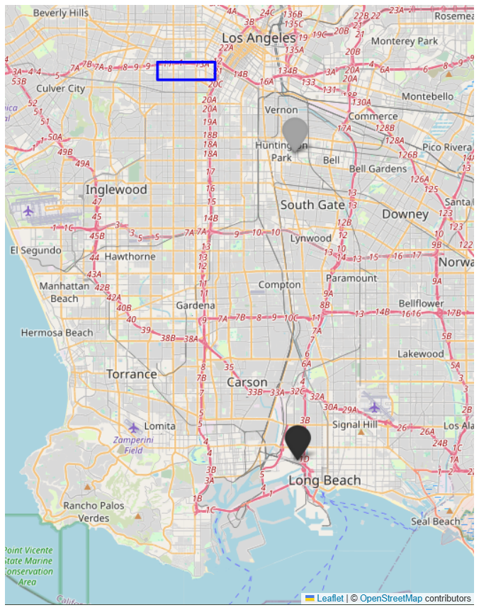
Figure 1 The TVOC and BTEX colocation site is indicated by the black icon, while the NO₂ colocation site is indicated by the gray icon. The harmonization site and field sites are encompassed in the blue box. ©OpenStreetMap contributors 2025. Distributed under the Open Data Commons Open Database License (ODbL) v1.0.

2.1 Instrumentation

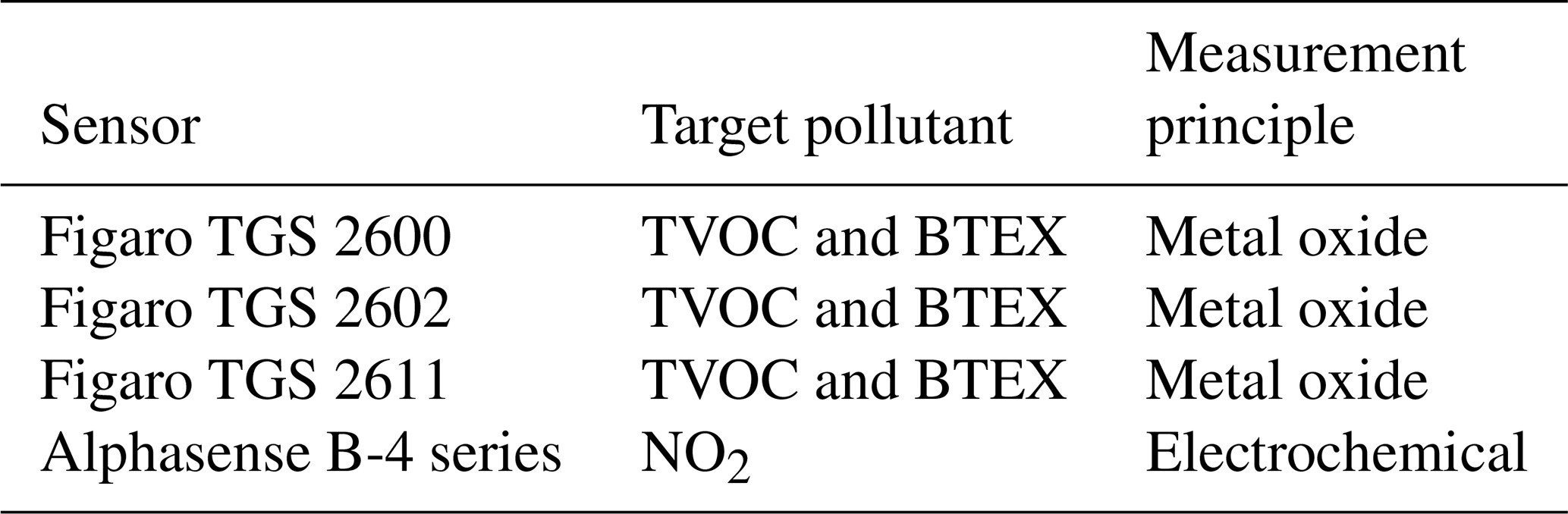
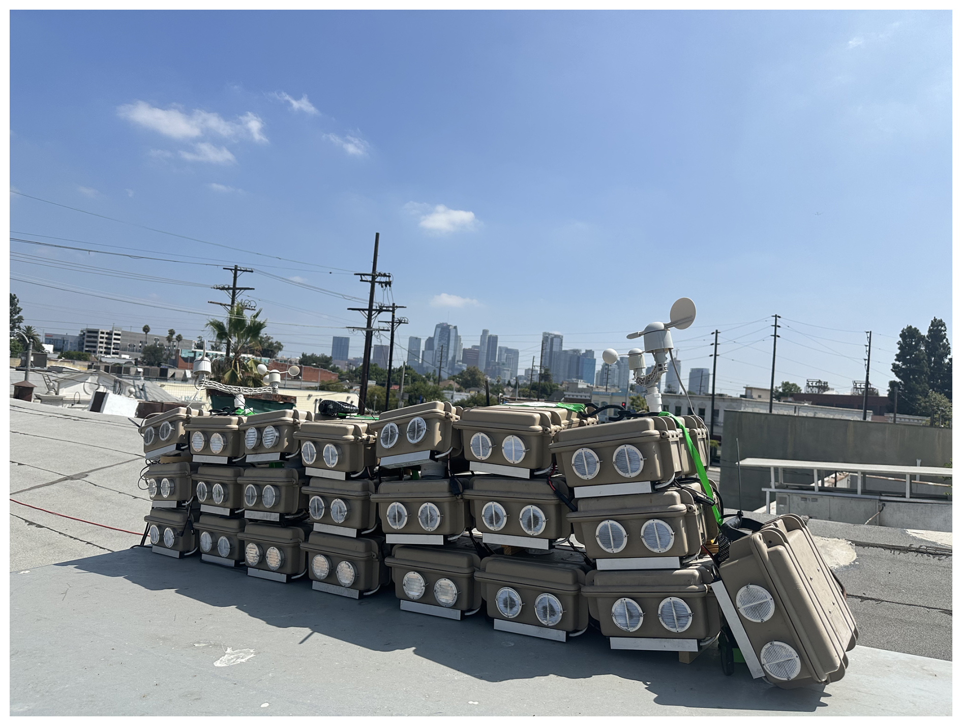
HAQ-Pods were developed in the Hannigan Air Quality (HAQ) Lab and have previously been used to capture local pollution events (Frischmon et al., 2025a; Silberstein et al., 2024). HAQ-Pods use interchangeable, commercial sensors to quantify various pollutants. The metal oxide and electrochemical sensors used in this study are listed in Table 1. We also used a Bosch BME 680 sensor for temperature and humidity measurements. The sensors are housed in a weather-proof case (10.7${}^{\prime \prime }\times {\mathrm{9.8}}^{\prime \prime }\times {\mathrm{4.8}}^{\prime \prime }$) outfitted with fans to draw air across the sensor surfaces. HAQ-Pods feature updated circuitry compared to Y-Pod air monitors, which have been described elsewhere (Collier-Oxandale et al., 2020, 2018).

Table 1 Sensors included in the HAQ-Pods.

For the TVOC calibration, the secondary standard HAQ-Pod was colocated with an Extractive Fourier Transform Infrared Spectrometer operated and maintained by the South Coast Air Quality Management District (South Coast AQMD) using methods similar to those described in Mellqvist et al. (2017). Ambient air is continuously drawn through heated Teflon inlet (1-inch ID) mounted on the roof of the station into a 25-liter cell at ∼25 L min⁻¹. Infrared light is generated with a glow-bar and directed into the cell with a series of mirrors. The light beam is passed through the cell multiple times via a series of curved mirrors to achieve a total path length of ∼100 m before exiting the cell and being directed into the infrared spectrometer (Bruker, Type: Matrix-M). Light is detected with an Indium/Antimonide detector in the 1800–4000 cm⁻¹ region and the spectrometer has a spectral resolution of 0.5 cm⁻¹.

Gas concentrations are calculated using synthetic spectra generated by fitting calibration spectra taken from the HITRAN (Sharpe et al., 2004) and PNNL (Rothman et al., 2005) databases to the raw spectra collected by the spectrometer in a linear least squares type fitting algorithm within the spectral evaluation window of 2725 to 3007 cm⁻¹ (Griffith, 1996; Johansson et al., 2014). The spectral fit includes calibration spectra for H₂O, CH₄, HDO, Propane, Butane, and Octane with TVOC reported as the sum of Propane, Butane, and Octane.

For the BTEX calibration, the secondary standard HAQ-Pod was collocated with an automated gas chromatograph (auto-GC) instrument (Tricorntech; MiTAP P320 Series) operated and maintained by South Coast AQMD. The auto-GC operates continuously with a distinct sampling and analysis phase that span 40 and 20 min, respectively. During the sampling phase, the auto-GC continuously draws ambient air at 5 cm³ min⁻¹ through a roof mounted inlet into a pre-concentrator for 40 min, totaling 200 cm³ of gas. During the analysis phase, the sample passes through a series of heated GC columns by way of pressurized inert carrier gas (N₂), where compounds are separated by polarity and subsequently detected with a series of photoionization detectors. Digital chromatograms are recorded and used to calculate ambient gas concentration via reference to a set of previously determined calibration chromatograms. Calibration chromatograms are determined by routinely (twice weekly) directing gas from a concentration-certified compressed cylinder into the auto-GC. The method is capable of an accuracy of 0.1 parts per billion by volume (ppbv).

For the NO₂ calibration, the secondary standard HAQ-Pod was colocated with a Teledyne T200 instrument maintained by the South Coast AQMD. The reference instrument was calibrated by the South Coast AQMD every six months and underwent weekly zero and span checks, in addition to nightly PC checks to ensure correct values.

2.2 Two-step colocation

The secondary standard HAQ-Pod was colocated with the South Coast AQMD instruments while all other HAQ-Pods were deployed at field sites in South Los Angeles from 10 October 2023 to 18 March 2024. The field HAQ-Pods were harmonized with the secondary standard HAQ-Pod from 4 to 9 October 2023 and from 18 to 28 March 2024. The physical set-up of the harmonization is shown in Fig. 2. Unlike previous two-step colocations, the HAQ-Pods were harmonized with the secondary standard both before and after field deployment to better account for sensor drift across the entire study period, as suggested by Sá et al. (2023).

Figure 2 Harmonization set up in Los Angeles

Sá et al. (2023) and Okorn and Hannigan (2021b) demonstrated different approaches for propogating the calibration model to the field LCSs in a two-step colocation (Fig. 3). Okorn and Hannigan (2021b) developed a primary calibration model between the secondary standard and reference instrument. In the harmonization step, the field LCS systems were then calibrated via a secondary calibration model to the concentration timeseries predicted by the calibrated secondary standard. This method is better suited for projects where the colocation and harmonization steps are similar in length, since each step requires equally complex calibration models.

Conversely, Sá et al. (2023) first developed a multi-linear regression model for each sensor signal corrected to the secondary standard's corresponding sensor signal. The multi-linear regression models for the pollutant sensors included temperature and humidity in addition to the pollutant sensor signal. The primary calibration model between the secondary standard and reference monitor could then be applied directly to the corrected field LCS systems. Since this method uses only a linear regression in the harmonization step, it is well-suited for projects where the harmonization is much shorter than the colocation. However, including temperature and humidity in the pollutant sensor regression model may introduce dependencies on environmental conditions that then require the harmonization step to span the full range of conditions expected in the field – thereby reducing the method’s usefulness for short harmonizations. To avoid this, we included only the pollutant sensor signal and a time elapsed variable in our linear regressions for harmonization, so that the regression corrects only for inter-sensor linear baseline shifts and drift (Eq. 1).

$$\begin{array}{}\text{(1)}& y_i={\mathit{\beta }}_{\mathrm{0}}+{\mathit{\beta }}_{\mathrm{1}}{x}_i+{\mathit{\beta }}_{\mathrm{2}}{T}_i+{\mathit{ϵ}}_i\end{array}$$

Where βs represent the model coefficients, x_i is the sensor signal for the ith observation, T_i is the time elapsed from the start of data collection for the ith observation, and ϵ_i represents the error term for the ith observation.

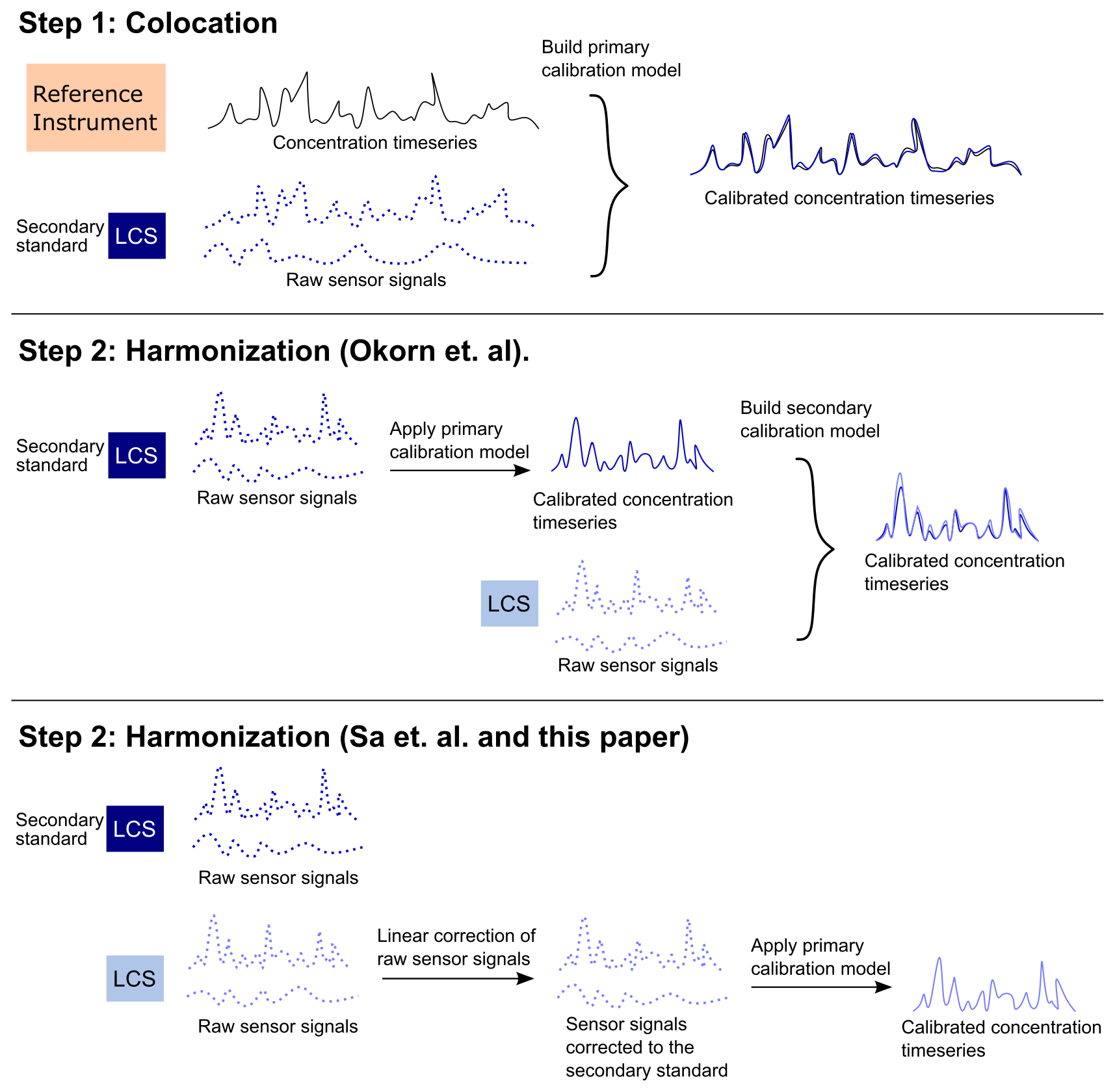
Figure 3 Model propogation methods for two-step colocation. This example has two sensor signal inputs: the target pollutant signal and temperature. Solid lines indicate a concentration timeseries and dotted lines indicate raw sensor signal. Note that Sá et al. (2023) include temperature and humidity in all linear correction models, while we include time elapsed in all linear correction models in this paper.

2.3 Calibration model development

Inputs into the TVOC and BTEX colocation calibration models included the signals from the metal oxide sensors, as well as temperature, humidity, and a time elapsed feature to account for sensor drift. The NO₂ calibration model used inputs from the electrochemical NO₂ sensor along with temperature, humidity, and time-elapsed data.

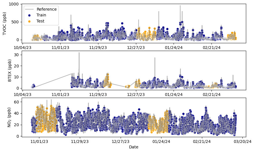
To evaluate model performance, we split the colocation data into training and testing datasets, allocating 80 % for training and 20 % for testing. While this train/test split is typically performed once, we repeated the calibration process 20 times to assess model robustness. For each run, we used a different split of the data. Specifically, for each iteration, we randomly selected a starting point in the time series and designated the next 10 % of data as testing data. A second 10 % segment was selected from a point halfway through the dataset relative to the first chunk, wrapping around if necessary. Figure 4 shows an example test/train split for each pollutant with reference and predicted concentrations (using a linear regression model) to demonstrate how this test/train approach allows the testing data to span different times of the year. This approach ensures the model is not overfit to a specific environmental state or season, while minimizing information leakage from autocorrelation between training and testing datasets (Nowack et al., 2021).

Figure 4 Example of the test/train split for each colocation timeseries.

The sensor signals are time averaged to 60-minute intervals prior to model training to reduce noise (Cabello-Solorzano et al., 2023). Signals were then z-scored to a mean zero and standard deviation equal to one based on the training data. During model training, we use k-fold cross-validation (k=5) to tune hyper-parameters to values that minimize the loss function, or mean squared error (MSE), shown in Eq. (2). We used the Scikit-learn Python module for all models except the artificial neural network, which used Tensorflow, and extreme gradient boosting, which used the Xgboost package.

$$\begin{array}{}\text{(2)}& \text{MSE}={\displaystyle \frac{\mathrm{1}}{n}}\sum _{i=\mathrm{1}}^n(y_i-{\widehat{y}}_i{)}^{\mathrm{2}}\end{array}$$

Where y_i is the reference concentration for the ith observation and $\widehat{y_i}$ is the predicted concentration for the ith observation, and n is the number of observations.

2.4 Machine learning model descriptions

2.4.1 Linear regression (LR)

LR employs the following expression to predict the reference concentration using the input sensor signals:

$$\begin{array}{}\text{(3)}& y_i={\mathit{\beta }}_{\mathrm{0}}+{\mathrm{\Sigma }}_{j=\mathrm{1}}^p{\mathit{\beta }}_j{x}_{ij}+{\mathit{ϵ}}_i\end{array}$$

Where βs represent the model coefficients, y_i is the reference concentration for the ith observation, x_ij is the jth feature or input for the ith observation, p is the number of features or model inputs, and ϵ_i represents the error term for the ith observation.

The model coefficients are tuned by minimizing the model error. There are no hyper-parameters that require tuning via k-fold cross-validation in a linear regression model.

2.4.2 Regularized linear regression: Lasso (L) and ridge (R)

Lasso (L) and ridge (R) are regularized linear regression models that add a penalty term to the loss function to reduce overfitting. Lasso uses L1 regularization, which adds the sum of the absolute values of the regression coefficients to the loss function (Eq. 4) (Tibshirani, 1996). This reduces the coefficients of unimportant inputs to zero, removing them from the model. Lasso regression is useful when it is suspected that not all model inputs are important for prediction. In ridge regression (L2 regularization), the penalty term is the sum of the squared values of the model coefficients (Eq. 5), which reduces the coefficients towards zero without setting them at zero (Hoerl and Kennard, 1970). Thus, ridge regression simplifies the model while retaining all inputs in the model.

$$\begin{array}{}\text{(4)}& {\displaystyle }& {\displaystyle }\text{Lasso loss Function}={\displaystyle \frac{\mathrm{1}}{n}}\sum _{i=\mathrm{1}}^n(y_i-{\widehat{y}}_i{)}^{\mathrm{2}}+\mathit{\lambda }\sum _{j=\mathrm{1}}^p|{\mathit{\beta }}_j|\text{(5)}& {\displaystyle }& {\displaystyle }\text{Ridge loss Function}={\displaystyle \frac{\mathrm{1}}{n}}\sum _{i=\mathrm{1}}^n(y_i-{\widehat{y}}_i{)}^{\mathrm{2}}+\mathit{\lambda }\sum _{j=\mathrm{1}}^p{\mathit{\beta }}_j^{\mathrm{2}}\end{array}$$

Where y_i is the reference concentration for the ith observation, $\widehat{y_i}$ is the predicted concentration for the ith observation, β_j is the coefficient for the jth model input, and λ is the regularization hyper-parameter, which determines the strength of the regularization.

2.4.3 Ensemble decision tree-based models: Random forest (RF), gradient boosting (GB), and extreme gradient boosting (XGB)

Random forest (RF), gradient boosting (GB), and extreme gradient boosting (XGB) are ensemble decision tree-based learning methods. Similarly to a flow chart, a decision tree separates the data into nodes based on the characteristics of the data, eventually reaching a final node that determines the prediction of the data (Song and Ying, 2015). As ensemble methods, these models combine outputs from multiple trees to produce a more robust solution (Breiman, 2001; Natekin and Knoll, 2013). RF uses a bootstrap aggregating approach (bagging) to combine the trees, where each tree is built independently and given equal weight in the final solution (Kumar and Sahu, 2021; Breiman, 2001). In contrast, GB and XGB use a “boosting” technique, where trees are built sequentially and seek to improve upon the error of the prior tree (Kumar and Sahu, 2021; Natekin and Knoll, 2013). XGB is a faster, optimized version of GB that also adds regularization (lasso and ridge) to reduce overfitting (Chen and Guestrin, 2016).

2.4.4 Support vector machine regression (SVR)

Support vector machine regression (SVR) maps the data to a high-dimensional space using a kernel function and determines the best-fitting hyperplane for the transformed data (Smola and Schölkopf, 2004). SVR minimizes the model complexity by only fitting the hyperplane to points falling outside a margin of tolerance. This is different than other machine learning models, which seek to minimize overall error across all data points.

2.4.5 Artificial neural network (ANN)

An artificial neural network (ANN) is a machine learning model designed to mimic the way input signals are processed and transformed into output signals in the brain (Wesolowski and Suchacz, 2012). In an ANN, the input signals pass through interconnected layers of nodes. The connections between the nodes are assigned weights, which are adjusted as the model is trained to optimize the output signal accuracy (Zhang, 2016; Krogh, 2008).

2.5 Calibration model evaluation

We evaluated the overall fit of the calibration models using three performance metrics: root mean squared error (RMSE) (Eq. 6), mean bias error (MBE) (Eq. 7), and coefficient of determination (R²) (Eq. 8). We also evaluated RMSE and MBE by percentile groups to assess model fits across the entire range of data. For the percentile-based assessment, the data were partitioned into 0–5th percentile, 5–25th percentile, 25–75th percentile, 75–95th percentile, and 95–100th percentile groups.

$$\begin{array}{}\text{(6)}& {\displaystyle }& {\displaystyle }\text{RMSE}=\sqrt{{\displaystyle \frac{\mathrm{1}}{n}}\sum _{i=\mathrm{1}}^n(y_i-{\widehat{y}}_i{)}^{\mathrm{2}}}\text{(7)}& {\displaystyle }& {\displaystyle }\text{MBE}={\displaystyle \frac{\mathrm{1}}{n}}\sum _{i=\mathrm{1}}^n(y_i-{\widehat{y}}_i)\text{(8)}& {\displaystyle }& {\displaystyle }{R}^{\mathrm{2}}=\mathrm{1}-{\displaystyle \frac{{\sum }_{i=\mathrm{1}}^n(y_i-{\widehat{y}}_i{)}^{\mathrm{2}}}{{\sum }_{i=\mathrm{1}}^n(y_i-\overline{y}{)}^{\mathrm{2}}}}\end{array}$$

Where y_i is the reference concentration for the ith observation and $\widehat{y_i}$ is the predicted concentration for the ith observation, and n is the number of observations.

Lastly, we applied the calibration models to sensor data collected from three field sites within the Los Angeles study area. We compare the predictions of each model to understand how they vary when applied to field conditions.

3 Results and Discussion

The full HAQ-Pod network included 11 field sites. We show data for just three sites to maintain the focus on sensor calibration in the present study. These three HAQ-Pods, along with the secondary standard HAQ-Pod had 100 % data completeness in the harmonization step, resulting in 333 harmonization data measurements for each HAQ-Pod after hourly averaging. Data completeness for HAQ-Pods 1, 2, and 3 in the field was 89 %, 86 % and 99 %, respectively, resulting in 3413, 3289, 3789 field data points for each HAQ-Pod. The secondary standard HAQ-Pod had 90 % data completeness, resulting in 3452 data points for the colocation calibration models.

3.1 Two-step colocation

As observed during harmonization, colocated HAQ-Pod raw sensor signals are generally well correlated, with correlation coefficients between the secondary standard HAQ-Pod raw signals and corresponding raw signals in the other HAQ-Pods ranging from 0.87 to 1 (Supplement). However, some shifted baselines and amplitudes are still visible in the left column of Fig. 5, especially for the metal oxide sensors, demonstrating the importance of correcting individual sensor signals rather than relying on a universal or general calibration. After applying the linear correction developed during harmonization (coefficients listed in Tables S2–S7), the signals are visually more aligned (right column of Fig. 5 and have correlation coefficients with the colocation HAQ-Pod signal ranging from 0.96–1 (Supplement).

The left column of Fig. 5 also reveals why performing both pre- and post-harmonization is essential for some sensors, especially Figaro TGS 2600 and 2611 in this case. These sensors show different behavior compared to the secondary standard HAQ-Pod signal in the pre- and post- harmonization, indicating sensor drift. We addressed this drift by including a time-elapsed feature in the harmonization correction, which approximates the drift as a linear function. It is likely the sensor drift is not perfectly linear, but the approximation appears to be sufficient here based on performance at both the start and end of harmonization. Conducting both pre- and post- harmonizations was essential for checking the drift approximation, as otherwise the model may extrapolate drift beyond what is reasonably possible.

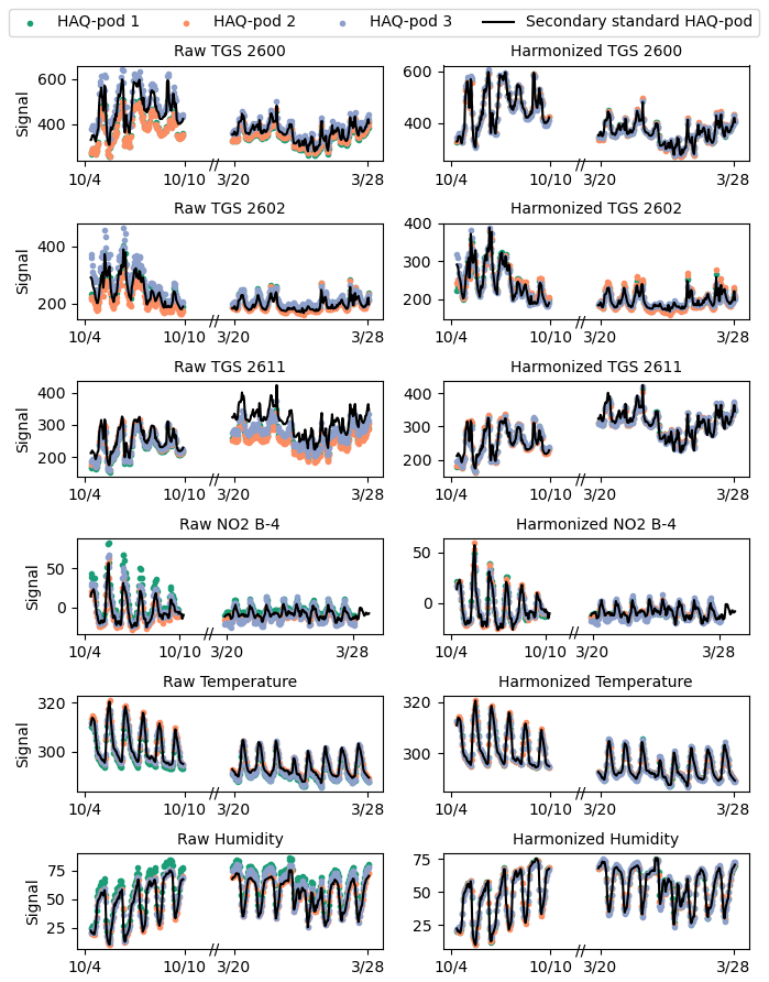
Figure 5 Raw sensor signal collected during harmonization (left column) and corrected signals after harmonization with the colocation HAQ-Pod (right column).

The temperature and humidity ranges recorded during the field deployment show strong overlap with the temperature and humidity ranges recorded at the HAQ-Pod colocation site (Fig. 6, note that measurements are uncalibrated sensor temperature and humidity). This overlap, which is important for colocation model transferability to field data, is possible because the two-step colocation allows for simultaneous colocation and field data collection. If colocation had occurred only before and after field deployment, as is typical for many low-cost sensor deployments, the overlap would look more like that of the field and harmonization phases in Fig. 6. Conditions during the harmonization phase trended towards higher temperature and humidity because the harmonizations occurred in fall and spring, while the field deployment was mainly in winter. This seasonal difference could lead to poor transferability if temperature and humidity impacts on the sensors were corrected in the harmonization phases because the model would have to extrapolate the impacts at low temperature and humidity ranges. Instead, our two-step colocation strategy corrects for sensor cross-sensitivity to temperature and humidity in the colocation phase only, where there is sufficient overlap of environmental conditions.

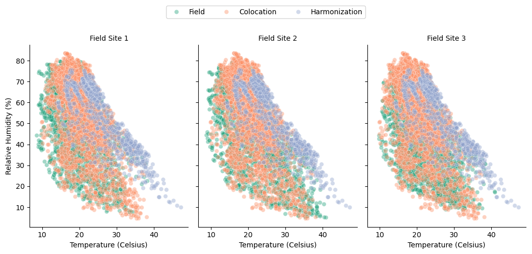
Figure 6 Relative humidity (RH) and temperature (T) observed during field (green), colocation (orange), and harmonization (purple) phases. These plotted values are harmonized sensor signals not calibrated to a true T or RH measurement.

3.2 Evaluation of machine learning calibration models

Figure 7 highlights how the distribution of TVOC and BTEX concentrations measured by the reference instruments during colocation are more skewed than NO₂, as 75 % and 78 % of the total concentration range falls within the 95–100th percentile group for TVOC and BTEX, respectively, compared with just 31 % for NO₂. Thus, the inclusion of NO₂ in our analysis provides a useful comparison of machine learning calibration performance on a more balanced dataset.

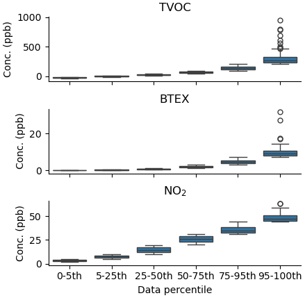
Figure 7 Reference concentrations, divided into data percentile ranges, of each pollutant collected during colocation.

In the following sections, we show the calibration model performance for each pollutant across all 20 calibration repetitions (Figs. 8, 11, 14). R² values for these models are available in Fig. S1. To better visualize how these models actually predict testing and field data concentrations, we show predicted data from one calibration run in Figs. 9, 10, 12, 13, 15, and 16. The calibration run we selected to visualize in these plots is one that was close to the median overall performance, based on RMSE and MBE, for each pollutant.

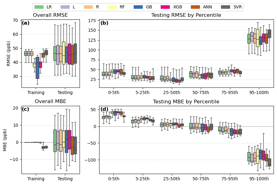
Figure 8 Performance statistics for TVOC calibration models, including overall RMSE (a), RMSE by percentile group (b), overall MBE (c), and MBE by percentile group (d). The calibration models are linear regression (LR), lasso (L), ridge (R), random forest (RF), gradient boosting (GB), extreme gradient boosting (XGB), artificial neural network (ANN), and support vector regression (SVR).

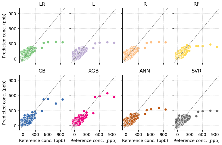
Figure 9 Predicted concentration versus reference concentration for TVOC calibration models: linear regression (LR), lasso (L), ridge (R), random forest (RF), gradient boosting (GB), extreme gradient boosting (XGB), artificial neural network (ANN), and support vector regression (SVR).

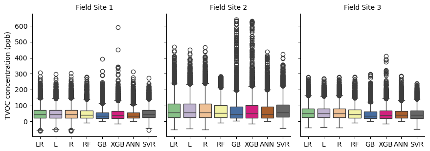
Figure 10 VOC concentration predictions at three field sites for each calibration model: linear regression (LR), lasso (L), ridge (R), random forest (RF), gradient boosting (GB), extreme gradient boosting (XGB), artificial neural network (ANN), and support vector regression (SVR)

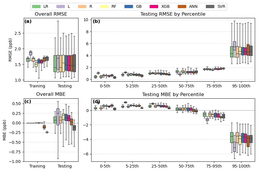
Figure 11 Performance statistics for BTEX calibration models, including overall RMSE (a), RMSE by percentile group (b), overall MBE (c), and MBE by percentile group (d). The calibration models are linear regression (LR), lasso (L), ridge (R), random forest (RF), gradient boosting (GB), extreme gradient boosting (XGB), artificial neural network (ANN), and support vector regression (SVR)

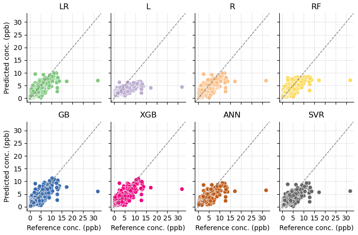
Figure 12 Predicted concentration versus reference concentration for BTEX calibration models: linear regression (LR), lasso (L), ridge (R), random forest (RF), gradient boosting (GB), extreme gradient boosting (XGB), artificial neural network (ANN), and support vector regression (SVR).

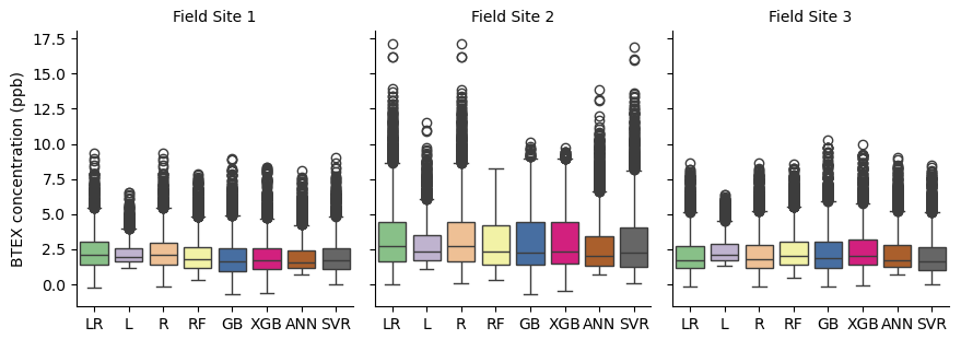
Figure 13 BTEX concentration predictions at three field sites for each calibration model: linear regression (LR), lasso (L), ridge (R), random forest (RF), gradient boosting (GB), extreme gradient boosting (XGB), artificial neural network (ANN), and support vector regression (SVR)

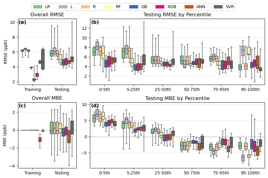
Figure 14 Performance statistics for NO₂ calibration models, including overall RMSE (a), RMSE by percentile group (b), overall MBE (c), and MBE by percentile group (d). The calibration models are linear regression (LR), lasso (L), ridge (R), random forest (RF), gradient boosting (GB), extreme gradient boosting (XGB), artificial neural network (ANN), and support vector regression (SVR)

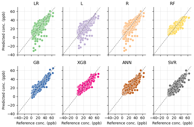
Figure 15 Predicted concentration versus reference concentration for NO₂ calibration models: linear regression (LR), lasso (L), ridge (R), random forest (RF), gradient boosting (GB), extreme gradient boosting (XGB), artificial neural network (ANN), and support vector regression (SVR).

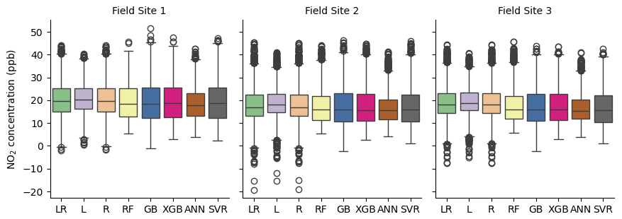
Figure 16 NO₂ concentration predictions at three field sites for each calibration model: linear regression (LR), lasso (L), ridge (R), random forest (RF), gradient boosting (GB), extreme gradient boosting (XGB), artificial neural network (ANN), and support vector regression (SVR)

3.2.1 TVOC calibration

Depending on the test/train split of the data, the overall RMSE and MBE for each model varied by 25–35 ppb (Panels A, C in Fig. 8). Within each run, the models showed similar overall testing RMSE and MBE, indicating the calibration performance depended more on test/train split than model choice. R² for all the models were also generally similar, with a median value of around 0.65 across all runs (Fig. S1). All the models tended to overestimate baseline concentrations in the 0–5th percentile, with the linear models showing the least overestimation bias (Fig. 8, panel d). The models also tended to underestimate peak concentrations in the 95–100th percentile, though gradient boosting (GB) performed best for these peak values based on its median MBE.

Linear regression (LR) and ridge regression (R) have nearly identical performance statistics, indicating that ridge, or L2, regularization of the linear model is not necessary for this data. Lasso, or L1, regularization removed humidity and time elapsed from the model inputs in 16 of 20 runs, removed temperature in one run, temperature and time elapsed in one run, and just time elapsed in two runs. None of these combinations significantly changed the model's performance compared to LR and R.

Visual inspection of the scatter plots in Fig. 9 shows that all models except the two boosting models, GB and XGB, severely underpredict the five highest concentrations. Boosting models are known to better predict extreme values in a regression model. These results suggest that boosting models are a good choice for applications where accurately capturing extreme concentrations is critical, such as pollution episode detection.

When applied to field data, the models predict similar mean concentrations, within a few parts per billion, but vary more in their predictions of extreme concentrations (baseline and peak) (Fig. 10). For the most part, this variation reflects the models performance on testing data. For example, LR, L, R, and SVR predict a negative baseline, which is also evident in the testing data predictions for these models, though less pronounced (Fig. 9). The boosting models (GB, XGB) consistently predict the highest maximum concentration, which is reflective of these models' performances in the 95–100th percentile of testing data. Overall, the models are correlated in their predictions, with correlation coefficients ranging from 0.88 to 1 between each model (Supplement).

3.2.2 BTEX calibration

The BTEX calibration models show little variability in performance across different test/train splits, except for data above the 95th percentile, where RMSE varied more than 5 ppb and MBE varied by more than 3 ppb for all models (Fig. 11). R² was the lowest of the three pollutants, with a median value of around 0.55 across all runs and models (Fig. S2). Lasso (L) had the worst performance overall, while the other two linear models (LR, R) show slightly better performance at the highest percentile and have the best overall RMSE and MBE.

SVR shows less overestimation of baseline concentrations (0–25th percentile) than the other models. Comparing this model to ANN in Fig. 11 reveals an important issue regarding overall MBE as a performance statistic. Both models show similar bias above the 50th percentile. However, ANN overpredicts lower concentrations (0–50th percentile) much more than SVR. As a result, ANN has a better overall MBE compared to SVR. This is important to consider because in a practical sense, a model that shows less overall bias by equally overpredicting the baseline and underpredicting peak values may not be more useful than a model that accurately predicts baseline concentrations but underpredicts peaks.

Figure 12 shows how the L model predicts far less variability than other models, with few data points predicted above 5 ppb. The L1 regularization used in L removed all inputs except TGS 2602, resulting in a poor model. The L2 regularization in R did not significantly change the model compared to LR.

Like TVOC, the mean concentrations predicted at each field site show little variation between models, but variation is higher when comparing the entire range of data (Fig. 12). L consistently has the smallest interquartile range, reflecting the lower variability predicted in the testing data. At sites 1 and 3, all models except L predict similar maximum concentrations. However, at site 2, RF, GB, and XGB predict much lower maximums than LR, R, ANN, and SVR. It is not clear why this inconsistency is occurring; however, it may indicate issues with transferability of the models for BTEX given their changing behavior across field sites. Overall, the models are still highly correlated with each other, with correlation coefficients between models at each field site ranging from 0.89 to 1 (Supplement).

3.2.3 NO₂ calibration

Overall, all the NO₂ calibration models tend to overpredict concentrations below the 25th percentile and underpredict concentrations above the 50th percentile (Fig. 14, panel d). However, underprediction of data above the 95th percentile is much less severe than TVOC and BTEX predictions, likely because the distribution of reference NO₂ concentrations is more balanced than the BTEX and TVOC concentration distributions, resulting in a much smaller range of peak concentrations to predict. RMSE remains much more consistent across percentiles for NO₂ compared to TVOC and BTEX (Fig. 14, panel b).

The three linear-based models (LR, L, R) perform poorly for NO₂, particularly in the low percentile range of concentrations, where the models predict negative concentrations (Fig. 15). Mean R² values were below 0.8 for these models, but mean R² for the non-linear models were above 0.8 (Fig. S3). L1 regularization in the L model removes temperature. The poor performance of L across the high and low percentile ranges compared to LR indicates that all inputs (NO₂ target sensor, temperature, humidity, and time elapsed) are necessary for this calibration.

Once again, differences in the field predictions between each model exist mainly in the extreme values (Fig. 16). As expected from testing data performance, the linear models predict some highly negative concentrations. RF is also consistent with its testing performance, specifically its baseline overestimation, as it shows the highest minimum concentration for all three sites. The correlation coefficients between a linear model (LR, R, L) and a non-linear model (RF, GB, XGB, ANN, SVR) are lower (0.73–0.93) than the correlation coefficients between two linear or two non-linear models (0.89–1) (Supplement). This is likely because of the unique negative concentrations predicted by the linear models.

3.3 Discussion

Across the three pollutants, the calibration models generally underestimated peak concentrations and overestimated baseline levels, though the extent of this bias varied with the distribution of the reference data. For TVOC and BTEX, which had more imbalanced distributions, peak underestimation was more pronounced, likely due to the wider range of high concentrations. These results highlight the importance of evaluating model performance across the full concentration distribution, rather than relying solely on overall metrics. In many cases, biases at the extremes were masked in the overall statistics because the baseline overestimation and peak underestimation often offset each other around the median, resulting in overall MBE values near zero.

While there was broad variability in model performance across pollutants, some patterns still emerged. For example, our results also showed nearly identical performance for linear regression (LR) and ridge regression (R) across the three pollutants, suggesting that L2 regularization was not beneficial for these datasets. Lasso regression also did not lead to improved predictive performance for linear regression, especially for BTEX and NO₂, where removing features through L1 regularization actually worsened model performance. To better understand the importance of each feature in response to the lasso performance, we plot the feature importances from the ensemble decision tree-based models (RF, GB, and XGB) in Fig. 17. The feature importances were calculated using the Mean Decrease in Impurity using the Scikit-learn Python module. Based on Fig. 17, it is clear that the target pollutant sensor features were more important than the temperature, humidity, and time elapsed features across all pollutants. However, given the reduced performance of lasso regression for BTEX and NO₂, it appears that even “less important” features can still play an essential role in model training. The increased importance of TGS 2602 for BTEX compared to TVOC aligns with previous work, which found TGS 2602 to be more sensitive to BTEX than TGS 2600 (Collier-Oxandale et al., 2019).

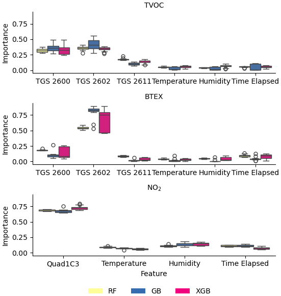
Figure 17 Feature importance for ensemble decision tree-based models (RF, GB, XGB) models for TVOC, BTEX, and NO₂.

Boosting methods, which are known for their improved ability to handle imbalanced data, reduced the underestimation of peak concentrations for TVOC. However, for BTEX, linear-based models (LR and R) actually outperformed boosting methods and other complex machine learning models for both peak concentrations and overall performance. For NO₂, the linear models performed the worst, especially at baseline concentrations, highlighting that no single model consistently performs best across all colocation datasets. When applied to field data, the models predicted similar mean concentrations for each site but had more variability in baseline and peak concentration predictions. Generally, the variability followed patterns evident in the testing data performance.

We built each calibration model multiple times, with differing test/train splits, to assess the robustness of each model. The performance metrics showed some variability, especially in the 95–100th percentile for BTEX and TVOC, based on the test/train split. This was not surprising, given that the range of concentrations in the 95–100th percentile for the BTEX and TVOC testing data could vary dramatically depending on the test/train split. These results motivate further study into how data should be split into testing and training sets to ensure transferability and robustness. At a minimum, we suggest ensuring that the testing data encompass the full range of concentrations measured during colocation.

4 Conclusions

Combining the two-step colocation process with a robust evaluation of multiple machine learning models led to satisfactory calibration of TVOC, BTEX, and NO₂ sensors in this study. Our two-step colocation strategy supported model transferability by ensuring the colocation encompassed more similar environmental conditions than was possible with only a pre- and post- calibration. We also showed why a two-step colocation is preferable to a universal calibration model, as the harmonization step was able to correct for the variability and drift unique to each individual sensor in a network. We found that calibration model performance is not one-size-fits-all and is affected by the distribution of reference concentrations and the test/train split. Even for models with little overall bias, percentile-based analysis revealed systemic overestimation of baseline concentrations and underestimation of peaks across all eight models: linear regression, lasso, ridge, random forest, gradient boosting, extreme gradient boosting, artificial neural network, and support vector regression.