A hybrid optimal estimation and machine learning approach to predict atmospheric composition

We present a HYbrid REtrieval Framework (HYREF) that predicts subcolumn carbon monoxide (CO) concentrations from Cross-track Infrared Sounder (CrIS) observations, trained to replicate the TRopospheric Ozone and its Precursors from Earth System Sounding (TROPESS) retrievals based on optimal estimation (OE). Unlike the OE algorithm, which produces retrievals for only a small fraction of available CrIS observations due to computationally expensive but physically accurate radiative transfer, the addition of machine learning (ML) techniques enables full coverage by providing high-resolution predictions for every valid CrIS sample. Importantly, in addition to CO concentrations, TROPESS-HYREF also predicts key retrieval diagnostics, namely column averaging kernels, degrees of freedom, and retrieval errors, that are essential for meaningful comparison with other observations, models, and ingestion into data assimilation. The framework is designed to emulate and extend the OE retrieval, rather than replace it, by providing full spatial coverage and enhanced resolution consistent with the underlying physical solution.

The new framework achieves excellent performance with correlation coefficients r>0.99 and a bias <0.1 % when benchmarked against an independent test set, and reproduces fine-scale spatial patterns in CO fields observed during a major wildfire over North America. A scale analysis reveals substantial variability in CO concentrations below the nominal 0.80° resolution of the TROPESS OE retrieval, which TROPESS-HYREF successfully resolves. Inference is computationally efficient, with daily global predictions completed in minutes on a single compute node. By filling observational gaps while maintaining consistency with the OE retrieval, this fusion of OE-derived physical information and ML-driven efficiency provides a practical pathway to high-resolution atmospheric CO monitoring with robust diagnostics.

1 Introduction

Carbon monoxide (CO) is a chemically reactive trace gas and key atmospheric pollutant, produced primarily through incomplete combustion of biomass and fossil fuels (Jacob, 1999), as well as through secondary production from the oxidation of methane (CH₄) and non-methane hydrocarbons (e.g. Holloway et al., 2000). It plays a central role in atmospheric chemistry by serving as a major sink for hydroxyl radicals (OH, Lelieveld et al., 2016), thereby influencing the oxidative capacity of the atmosphere and the lifetime of CH₄ (e.g. Gaubert et al., 2017). Due to its intermediate lifetime (weeks to months), CO serves as a valuable tracer for long-range pollution transport and chemical processing in the troposphere (e.g. Clerbaux et al., 2002; Edwards et al., 2004). It also contributes indirectly to radiative forcing via the formation of tropospheric ozone (O₃) and carbon dioxide (CO₂), classifying it as a short-lived climate pollutant (Bowman and Henze, 2012; IPCC, 2023).

Satellite observations of CO, beginning with the Measurements of Air Pollution from Satellites (MAPS, Reichle Jr. et al., 1990) in the early 1980s and continuing with instruments such as Measurement of Pollution in the Troposphere (MOPITT) (Drummond et al., 2010), Atmospheric Infrared Sounder (AIRS) (Aumann et al., 2003), Tropospheric Emission Spectrometer (TES) (Beer et al., 2001), Infrared Atmospheric Sounding Interferometer (IASI) (Clerbaux et al., 2009), Cross-track Infrared Sounder (CrIS) (Han et al., 2013), TROPOspheric Monitoring Instrument (TROPOMI) (Veefkind et al., 2012), Greenhouse Gases Observing Satellite 2 (GOSAT–2) (Noël et al., 2022) and Geostationary Interferometric Infrared Sounder (GIIRS) (Zeng et al., 2023), have provided a long-term, global perspective on CO distributions, emission sources, and trends (e.g. Worden et al., 2013; Buchholz et al., 2021). These datasets support air quality monitoring, inverse modeling of emissions, and evaluation of chemistry-climate models (e.g. Field et al., 2015, 2016; Buchholz et al., 2018). While global CO concentrations have declined over the past two decades due to improved combustion efficiency and decreased biomass burning (e.g. Schultz et al., 2015; Zheng et al., 2019), recent regional fire trends (see, e.g. Luo et al., 2024), and evolving air quality policies continue to shape CO variability, underscoring the need for sustained satellite observations with well-characterized uncertainties (e.g. Strode et al., 2016). Nevertheless, changes in climate and extreme events can lead to substantial biomass burning events for which CO is a critical tracer to infer emissions (Byrne et al., 2021, 2024; Neyra-Nazarrett et al., 2025).

The NASA TRopospheric Ozone and its Precursors from Earth System Sounding (TROPESS) project generates consistent, long-term records of tropospheric ozone and related trace gases, including CO (Bowman, 2021; Worden et al., 2022). Building on the TES legacy, TROPESS applies a unified optimal estimation (OE, see, e.g. Rodgers, 2000) algorithm across multiple satellite platforms, supported by a comprehensive ground data system (Bowman et al., 2006; Fu et al., 2016). Emphasis is placed on rigorous uncertainty analysis and intercomparisons with independent observations to ensure the accuracy needed for trend detection. Figure 1a shows the spatial distribution of operational TROPESS Level 2 (L2) CO retrievals over the western US on 10 June 2023, based on CrIS measurements. A regional zoom (red box) reveals that, due to computational constraints, only ≈1.5 % of the available CrIS soundings are processed, leaving substantial gaps in global CO monitoring.

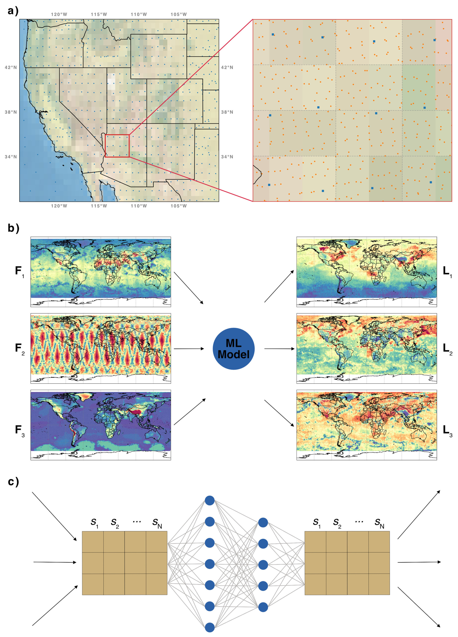
Figure 1 (a) Geolocations of L2 CO retrievals (blue dots) and L1B CrIS radiances (orange dots) over the western US on 10 June 2023. (b) Simplified sketch of the ML setup, where three features (F_1–3; radiances at 2181.88 cm⁻¹, sensor viewing angle, and surface altitude) are used as input for the ML model in order to predict three labels (L_1–3; CO concentrations, retrieval error, and an individual column averaging kernel). (c) Simplified sketch of the ML model. The variables F_1–3 are converted to a two-dimensional input matrix which connects to neurons in two hidden layers, and map to a two-dimensional output matrix, which provides L_1–3.

Machine learning (ML) approaches, whose use in atmospheric science has expanded in recent years (e.g. Grivas and Chaloulakou, 2006; Saponaro et al., 2013; Werner et al., 2020, 2023; Schultz et al., 2021), offer a promising path forward. ML models can efficiently learn complex, nonlinear relationships and provide rapid inference across large datasets. However, limitations in explainability and uncertainty quantification continue to hinder their broader application in remote sensing (Tyralis and Papacharalampous, 2024).

In contrast to conventional OE retrievals, which produce not only the retrieved quantities of interest but also key diagnostics such as χ² statistics, degrees of freedom (DoF), retrieval precision, error covariance, and column averaging kernels (AK), ML methods lack direct analogues to these quantities. Yet such diagnostics are critical for model-observation comparisons, data assimilation, and quality control (Jones et al., 2003; Miyazaki et al., 2015; von Clarmann and Glatthor, 2019).

Here, we present a novel hybrid framework that combines the strengths of OE and ML to generate high-resolution estimates of CO column concentrations from CrIS radiances. Our approach leverages OE retrievals as both training targets and sources of physically meaningful prior information, while enabling ML-driven capabilities such as rapid upscaling and the emulation of retrieval diagnostics. This fusion fills observational gaps left by current processing limits and provides an interpretable, uncertainty-aware pathway for incorporating ML into operational remote sensing pipelines. Importantly, the ML component is designed to emulate the OE retrieval and its associated diagnostics, rather than to replace or surpass the underlying physical solution, thereby extending OE-derived information to full spatial coverage. The TROPESS-HYREF framework is therefore intended as a hybrid OE-ML system, in which the ML model operates alongside OE, for example by filling gaps in retrieval coverage, and can be periodically retrained as new OE results become available.

2 Data

The CrIS instrument, onboard NOAA's Joint Polar Satellite System–1 (JPSS–1, also known as NOAA-20), is a Fourier Transform Spectrometer that captures Earth views across 30 cross-track interferograms, providing a swath width of 2200 km. Each interferogram contains a 3×3 array of fields of view (FOVs), with each circular FOV having a diameter of 14 km at nadir. CrIS data are processed to provide calibrated Level 1B (L1B) radiances in three spectral bands: 660–1095 cm⁻¹ (longwave), 1210–1750 cm⁻¹ (midwave), and 2155–2550 cm⁻¹ (shortwave). The instrument unapodized spectral resolution is 0.625–2.5 cm⁻¹. NASA's version 2 L1B radiances are available from the Goddard Earth Sciences Data and Information Services Center (GES DISC) UW-Madison Space Science and Engineering Center: Hank Revercomb; UMBC Atmospheric Spectroscopy Laboratory: Larrabee Strow, 2018.

TROPESS trace gas retrievals are provided on a reduced horizontal grid of 0.8° by the MUSES data processing system (Fu et al., 2016, 2018, 2019). These retrievals are based on the TES L2 processing algorithm (Bowman et al., 2006) and utilize an OE retrieval approach (Rodgers, 2000). TROPESS retrievals of carbon monoxide (CO) are processed operationally, have undergone extensive verification (e.g. Worden et al., 2022; Luo et al., 2024), and are accessible via the GES DISC. In this study, single-FOV CrIS–MUSES retrievals from the TROPESS forward stream were used (Bowman, 2021).

Data in this study are comprised of CrIS and TROPESS data over April 2023–January 2025.

3 ML model

3.1 Setup and training

We developed, trained, and evaluated a ML model to simultaneously predict a variety of TROPESS CO variables, primarily using observed CrIS radiances and geolocation data as inputs. This setup is illustrated in the simplified diagram in Fig. 1b, where we drastically limit the input and output variables to aid visibility. In this example the model uses three features (F_1–3) as input: CrIS radiances at 2181.88 cm⁻¹, the sensor viewing angle, and the surface altitude, respectively. These features are matrices, where each element $f_{\text{1–3}}^s$ corresponds to one of the N samples, indexed as $s=\mathrm{1},\mathrm{\dots },N$. The ML model maps these features to a set of output labels (L_1–3), which in this simplified example are the CO total column concentrations, the total column retrieval error, and the column AK at ≈511 hPa. Like the features, these labels are matrices that contain elements $l_{\text{1–3}}^s$ for each individual sample. Again, $s=\mathrm{1},\mathrm{\dots },N$ denotes the individual sample (i.e. CrIS column).

The ML model developed in this study is a feedforward artificial neural network (ANN), which maps the input to the output through several hidden layers, each consisting of a large number of interconnected neurons. A simplified schematic of an example ANN, with two hidden layers containing 7 and 5 neurons, respectively, is shown in Fig. 1c. This diagram also illustrates how the geolocated features are transformed into two-dimensional input and output matrices and how they connect to the individual neurons.

The exact model structure and hyperparameters (i.e. model settings) are determined through the procedures described in Werner et al. (2021, 2023). By applying k fold cross-validation across a range of potential model setups, the ideal hyperparameters were found to be two hidden layers with 1506 neurons per layer, “Rectified Linear Unit” activation functions after each hidden layer, an L2 weight decay parameter of $\mathrm{5.00}\times {\mathrm{10}}^{-\mathrm{34}}$, and the “Adaptive Moment Estimation” optimizer with a learning rate of $\mathrm{1}\times {\mathrm{10}}^{-\mathrm{5}}$. The loss function minimized during training is the mean squared error. For each training iteration, batches of samples are passed through the model in a forward pass to compute predictions, followed by a backward pass in which model weights are updated via backpropagation. Each mini-batch contains 8192 samples. Further details on these parameters and their impact are provided in Reed and Marks (1999), Goodfellow et al. (2016), and Werner et al. (2021).

Model training was carried out using the “Keras” library for Python (version 2.10.0; Chollet et al., 2015), with “TensorFlow” (version 2.10.0) as the backend (Abadi et al., 2016). Of the available CrIS radiances and TROPESS retrievals over April 2023–January 2025, 98 % of randomly selected samples were used as training data. After each training iteration, the model's performance was evaluated for an independent validation dataset comprised of 1 % of the available data (approximately 185 000 samples). After several thousand iterations, the model weights corresponding to the best performance scores on the validation set were saved.

The specific features used for the CO model include radiances from all 2224 spectral channels, the FOV index, the latitude and longitude of each sample, UTC time, a day/night flag, the sensor viewing angle, the day of the year, and the TROPESS subcolumn a priori values. This yields an input matrix containing 2235 variables. Note that the surface altitude was included for models predicting retrievals and diagnostics for other TROPESS species. We tested reduced channel sets focused on CO-sensitive regions but found that using the full spectrum provided slightly improved performance, likely due to additional information on atmospheric state variables (e.g. temperature and humidity). The predicted labels of the CO model consist of the subcolumn concentrations, column AKs, and subcolumn retrieval errors, resulting in an output matrix containing 24 variables.

Prior to training, these inputs and outputs were filtered to remove invalid samples using a set of basic quality filters, including non-finite values, fill values, extreme outliers, failed retrieval quality flags, and target values outside the valid retrieval range. In addition, extreme outliers in the label distributions were masked using percentile-based tail cutoffs, and both input features and output labels were standardized before training.

Model training was performed on a high-performance computing cluster and took ≈10 d to converge to a solution for the >12 000 000 model weights.

3.2 Evaluation

Model performance is evaluated using an independent test dataset, which consists of the remaining 1 % of randomly sampled data that were not included in the training or validation process. Ideally, (i) the model should reliably predict CO concentration retrievals and OE diagnostics for these data points, even though the ML algorithm was not trained on them, and (ii) performance metrics should be similar to those derived from the training and validation datasets. It is important to note that the objective of the ML model is not to generalize beyond the statistical characteristics of the OE retrieval, but to emulate the OE solution and provide full spatial coverage for the same observing system. As such, the random split into training, validation, and test datasets ensures that the model is evaluated on samples that were not explicitly used during training, while still reflecting the same underlying distribution of atmospheric states and observational conditions. Given the strong spatial and temporal correlations inherent in satellite observations, this approach is appropriate for assessing the model's ability to reproduce OE retrievals across the full range of conditions encountered in the dataset. In operational use, the model is continuously retrained with newly available OE retrievals, ensuring consistency with evolving atmospheric variability.

Figure 2a presents a joint histogram of total column CO from the ML and OE algorithms for over 180 000 samples in the independent test dataset. Yellow colors represent regions with the highest density of data points, while blue colors correspond to areas with very few samples. The good agreement between the ML and OE results is evident, as most observations are narrowly clustered around the 1:1 line (indicated by the gray, dashed line). Five performance metrics are provided in the panel: Pearson's product-moment correlation coefficient (r), the root-mean-square deviation (RMSD), the median deviation between the predicted and retrieved CO (50p, i.e. the bias), and the 1st and 99th percentiles of the deviation. Notably, for the total column concentrations, we find r>0.99, $\text{RMSD}=\mathrm{3.11}\times {\mathrm{10}}^{\mathrm{16}}$ molecules cm⁻², a median difference of $-\mathrm{7.27}\times {\mathrm{10}}^{\mathrm{14}}$ molecules cm⁻², and maximum absolute differences for the majority of samples of $<\mathrm{1.00}\times {\mathrm{10}}^{\mathrm{17}}$ molecules cm⁻².

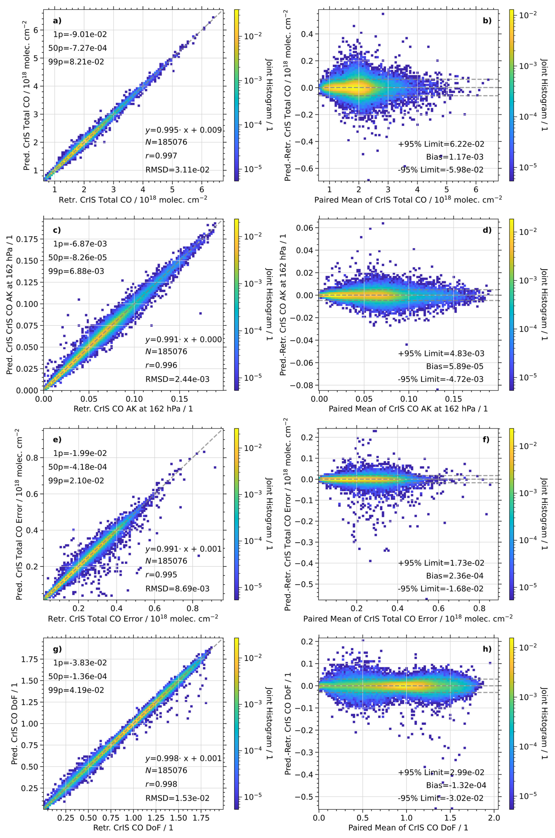
Figure 2 (a) Joint histogram and (b) Bland–Altman plot of predicted and retrieved total column CO concentrations from the test data set. (c)–(h) Similar to (a) and (b), but for the column averaging kernel (AK) at 162 hPa, total column retrieval error, and degrees of freedom (DoF).

Similar comparisons for tropospheric column concentrations, total AK at 162 hPa, and DoF are shown in Fig. 2c, e, and g. Again, the distributions closely follows the 1:1 line, with similarly high correlations (r>0.99). The lowest correlation occurs for the column AK at the lowest atmospheric level (not shown), where r=0.98. These performance metrics are almost identical to those obtained for the validation dataset, where the comparison of predicted and retrieved total column CO concentrations yields r>0.99, $\text{RMSD}=\mathrm{3.14}\times {\mathrm{10}}^{\mathrm{16}}$ molecules cm⁻², a median difference of 6.57×10¹⁴ molecules cm⁻², and maximum absolute differences for the majority of samples of $<\mathrm{1.00}\times {\mathrm{10}}^{\mathrm{17}}$ molecules cm⁻².

Performance metrics are consistent across training, validation, and test datasets, with nearly identical correlation coefficients ($\left|\mathrm{\Delta }r\right|<\mathrm{0.0006}$), normalized RMSD values ($\left|\mathrm{\Delta }\text{RMSD}\right|<\mathrm{0.21}\mathrm{\%}$, apart from the last two column AK levels deep in the stratosphere where values of effectively 0), and biases ($\left|\mathrm{\Delta }\text{bias}\right|<\mathrm{0.12}\mathrm{\%}$) for all predicted variables. This indicates that there is no evidence of overfitting and that the model exhibits stable behavior across the available datasets.

We note that the use of a random split does not enforce strict independence between training, validation, and test datasets, as atmospheric states exhibit strong spatial and temporal correlations. In this study, the purpose of the split is therefore not to assess fully independent generalization, but to evaluate how well the model reproduces OE retrieval behavior across the distribution of atmospheric states and viewing geometries sampled by the instrument.

To ensure that the split remains representative, we verified that the distributions of key variables are statistically consistent across training, validation, and test datasets using Kolmogorov–Smirnov tests. Combined with the consistent performance metrics reported above, this indicates that the model generalizes well within the sampled observational distribution. This behavior is consistent with the intended hybrid OE–ML application, in which the model is designed to operate on the same observational distribution as OE.

To complement the regression analysis, we employ Bland–Altman plots to further assess the agreement between the OE and predicted results. This approach highlights systematic differences and potential heteroscedasticity that may not be apparent in standard correlation-based evaluations, especially for non-Gaussian or magnitude-dependent variability, and has been shown to provide a more robust framework for intercomparison of geophysical datasets (e.g. Knobelspiesse et al., 2019). Panels b, d, f, and h show the Bland–Altman distributions, with the paired mean of predicted and OE values on the x axis and the difference between the two datasets on the y axis, along with three horizontal dashed lines. The central line denotes the mean difference (bias), while the outer lines show the 95 % limits of agreement (mean ±1.96 standard deviations), indicating the interval that contains approximately 95 % of the differences under the assumption of normally distributed residuals.

The distributions show no evidence of magnitude-dependent bias or systematic slope. The proportion of data points within the 95 % limits of agreement (95 %, 95 %, 96 %, and 95 %, respectively) aligns closely with expectations for normally distributed residuals, and 79 %, 80 %, 86 %, and 78 % of points fall within ±1 standard deviation. This indicates well-behaved error distributions with no pronounced evidence of heavy tails or heteroscedastic spread, suggesting that the model adequately captures variability across the full dynamic range. This is particularly relevant for machine learning retrievals, which can otherwise struggle in the presence of heteroscedastic relationships between observables and geophysical variables (e.g. Miller et al., 2020), and indicates that such effects are not evident in our ML predictions. Minor increases in spread near the peak of the distributions reflect regions of highest data density and do not indicate systematic bias or magnitude-dependent variability.

The close agreement between predicted and OE-derived diagnostics indicates that the ML model not only reproduces the retrieved state, but also captures the associated sensitivity and uncertainty characteristics of the OE solution. This consistency is critical for downstream applications, such as data assimilation and model evaluation, where the proper interpretation of retrievals depends on the availability of reliable AKs and error estimates.

4 Results

4.1 Example maps

Figure 3a presents a representative example scene of total column CO from the TROPESS OE retrieval on 10 June 2023. A large area of enhanced CO concentrations ($>\mathrm{3.00}\times {\mathrm{10}}^{\mathrm{18}}$ molecules cm⁻²) is evident over Western Canada, associated with the unprecedented wildfire season that year (Jain et al., 2024). These fires produced large smoke plumes that affected portions of Canada and the US for several weeks, before spreading across the Northern Hemisphere. Notably, enhanced CO concentrations ($>\mathrm{2.50}\times {\mathrm{10}}^{\mathrm{18}}$ molecules cm⁻²) are also recorded over Eastern Canada, the entire Eastern US, and parts of the Atlantic Ocean.

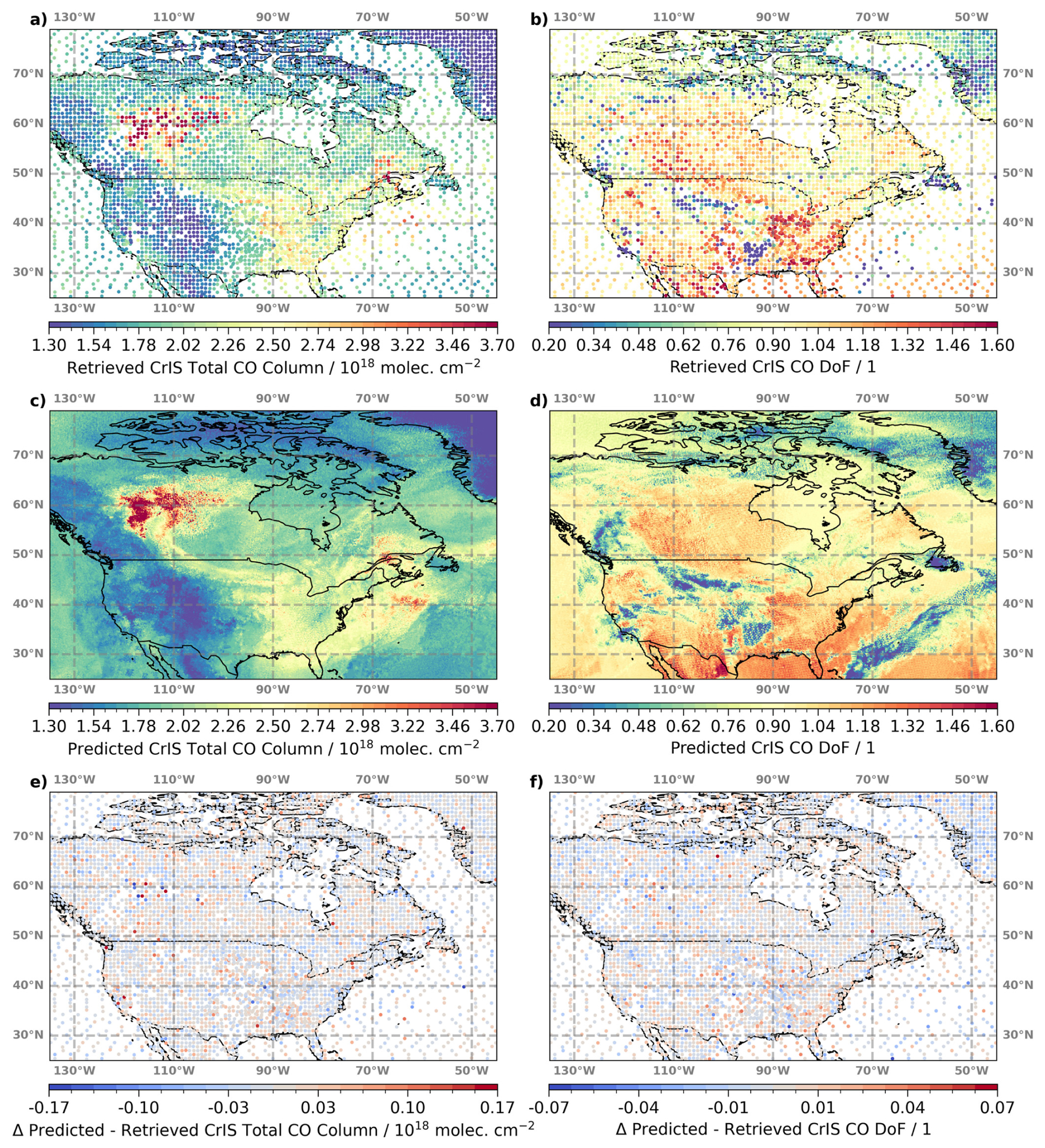
Figure 3 (a) Example scene of OE retrievals of total column CO over North America on 10 June 2023. (b) Similar to (a), but showing the associated OE degrees of freedom (DoF). (c, d) Similar to (a, b). but for the ML predictions. (e, f) Differences between colocated ML predictions and OE retrievals, and their respective error estimates.

The associated OE DoF are shown in Fig. 3b. Areas of moderate to high CO concentrations generally coincide with regions of elevated DoF. Smaller DoF<0.6 are observed over Greenland, the Atlantic Ocean, and over isolated regions over the continental US. These reduced DoF are indicative of lower retrieval sensitivity and are likely due to the interference of clouds or poor thermal contrast.

Figure 3c and d show the ML predictions for total CO concentrations and DoF, respectively. These results are derived for each CrIS L1B sample. The increased spatial resolution is particularly noticeable over the oceans, but even over land the ML results capture much finer spatial features, while faithfully reproducing the CO enhancements and DoF from the OE retrieval. Divergence maps in Fig. 3e and f illustrate the differences between predicted and retrieved results. The median differences are <0.1 % for both variables, and for the majority of samples (i.e. within the 5th and 95th percentiles), ML predictions are within ±2.40 % for total CO concentrations and within ±4.12 % for DoF. Overall, the difference between ML and OE total column CO concentrations exceeds the retrieval error for only 14 of the 5308 samples in the scene (0.26 %). Similarly, excellent agreement is observed for the retrieval errors (not shown), with a majority of ML predictions within ±6.11 % and a median difference of 0.04 %.

The close agreement between the ML predictions and OE retrieval shown in Fig. 3 primarily reflects interpolation within the sampled observational distribution, as this day is part of the training period, rather than fully independent spatiotemporal generalization. To further assess the performance of the ML model beyond the training period, Fig. 4 shows a global scene for 8 June 2025, which lies outside the training range (April 2023–January 2025). This experiment represents a limited temporal extrapolation test rather than a comprehensive assessment of long-term model stability. The results demonstrate that the model retains strong predictive skill under these conditions, indicating that it can generalize to unseen temporal states to a certain extent. However, we emphasize that such standalone predictive capability is not the primary objective of the framework. The model is designed to operate as part of a hybrid OE–ML system, benefiting from periodic retraining and remaining closely tied to the evolving distribution of OE retrievals.

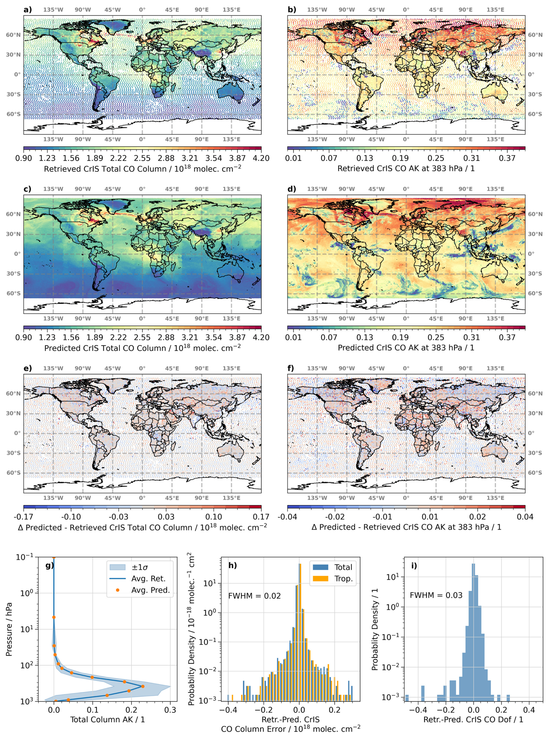
Figure 4 (a, c, e) Similar to Fig. 3a, c, and e, but showing global total column CO for 8 June 2025. (b, d, f) Similar to (a, c, e), but for the column averaging kernel (AK) at 383 hPa. (g) Global mean column AK profile as a function of pressure, showing OE results (blue), associated variability (±1σ, shaded), and ML predictions (orange). (h) Probability density functions of the difference between ML and OE total column retrieval errors (blue) and tropospheric column retrieval errors (orange). (i) Probability density function of the difference between ML and OE degrees of freedom (DoF). This scene lies outside the training period.

Similar to Fig. 3, the ML predictions reproduce the spatial structure of total column CO with high fidelity, including regions of enhanced concentrations associated with wildfire activity over North America. Differences between ML predictions and colocated OE retrievals remain small and spatially unstructured. The median difference is <0.13 %, and the majority of samples (again, within the 5th and 95th percentiles) has ML CO concentrations within ±3.00 % of the OE results.

In addition to column concentrations, Fig. 4 demonstrates that the ML model accurately reproduces key retrieval diagnostics. The column AK exhibit a maximum at 383 hPa and is shown in panels b, d, and f, showing strong agreement in both spatial structure and magnitude. The median difference is <0.67 %, and the majority of ML predictions lie within ±8.50 % of the OE results. The global mean AK profiles (Fig. 4g) are nearly identical between OE and ML, with differences well within the natural variability of the OE retrieval. Median differences over all vertical levels are within 0.001 % and 90 % of predictions are within 0.028 of the true AK value at any level. This translates to 1.5 % and 10 %, respectively, at levels where the AK is noticeably different from zero, i.e. in the troposphere above the surface.

Likewise, differences in retrieval errors (Fig. 4h) and degrees of freedom (Fig. 4i) are centered near zero and exhibit narrow distributions, with full-width-at-half-maximum values of 0.02×10¹⁸ $\mathrm{molec}.{\mathrm{cm}}^{-\mathrm{2}}$ and 0.032, respectively. This behavior indicates that the ML-predicted diagnostics are statistically consistent with those derived from OE, within the intrinsic variability of the retrieval.

Together, these results demonstrate that the ML framework not only reproduces the retrieved state, but also captures the associated sensitivity and uncertainty characteristics of the OE solution for unseen atmospheric conditions, while resolving finer spatial structures beyond the native OE sampling. These characteristics suggest that the predicted diagnostics retain the key properties required for downstream applications such as data assimilation, although a full assessment within an assimilation framework is beyond the scope of this study.

4.2 The added value from CO at higher spatial resolution

A key question is whether the ML product captures physically meaningful CO variability below the nominal 0.80° TROPESS retrieval resolution, or whether it primarily behaves as a spatial interpolation of the OE field. While interpolation can reconstruct smooth fields between observations, it cannot introduce new information at unresolved spatial scales.

To investigate this, we employ two complementary approaches: (i) comparing the ML-predicted CO fields with linearly interpolated TROPESS CO retrievals, and (ii) analyzing the spatial power spectral densities E_I(k) to identify scale-dependent variability, particularly in the sub-0.80° domain. Together, these approaches allow us to assess whether interpolation is sufficient to capture the underlying structure, or whether additional variability persists at smaller scales that requires the higher-resolution information provided by the ML model.

Figure 5a shows the interpolated OE CO retrievals. This field appears significantly smoother than the ML predictions (Fig. 3c), especially for the region of enhanced CO over Western Canada and the Northeastern US. The difference between the interpolated and predicted CO concentrations is illustrated in Fig. 5b, where blue and red colors indicate underestimation and overestimation by the interpolation, respectively. Deviations are centered around 0.50 % but can exceed ±30 %, especially in areas of enhanced CO. Maximum differences increase further, to ±48 % and ±58 %, when using nearest-neighbor or cubic spline interpolation, respectively.

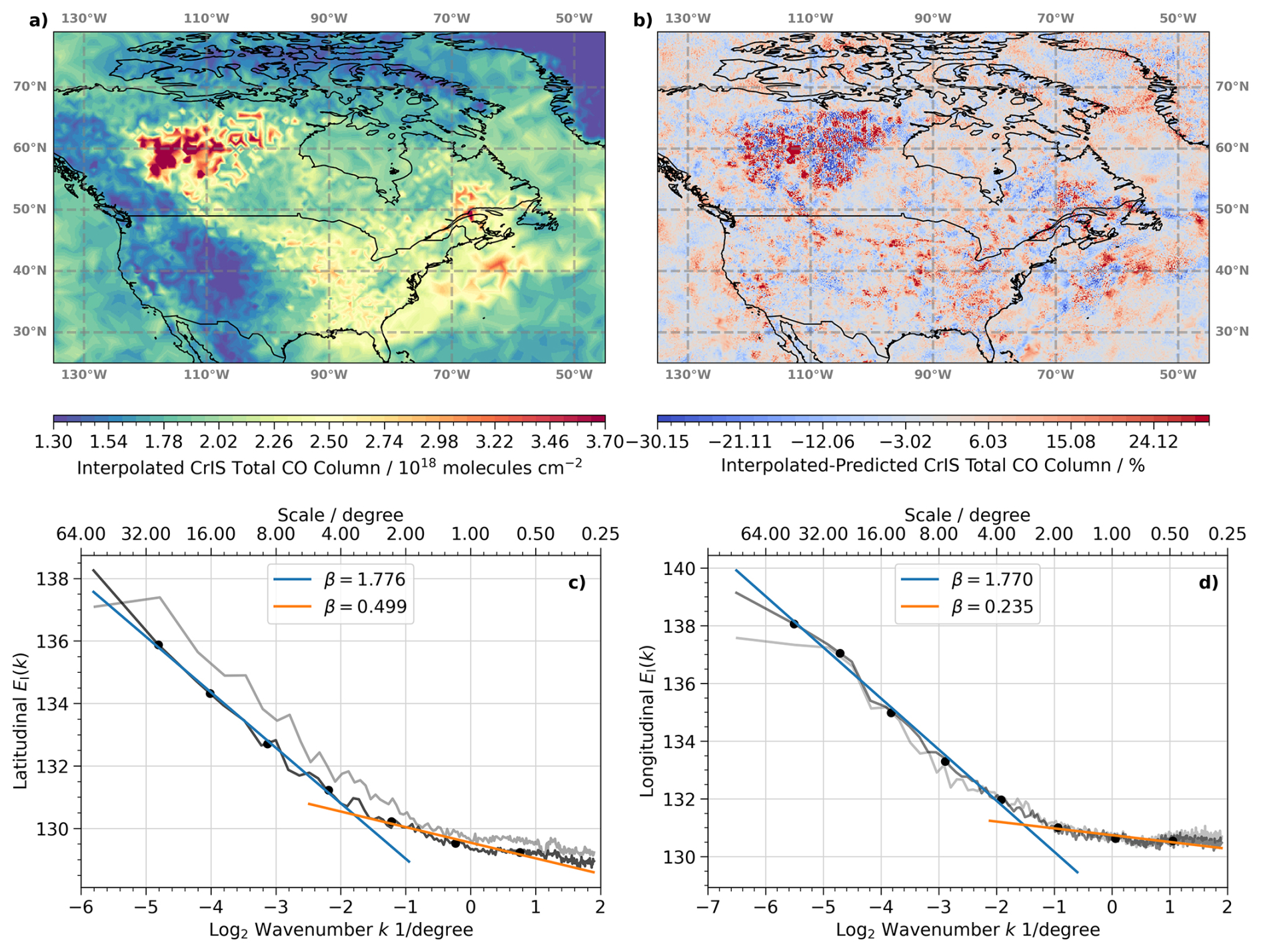
Figure 5 (a) Interpolated TROPESS total column CO on 10 June 2023. (b) Difference between interpolated and predicted CO. (c, d) Average power spectral density E_I(k) (black) as a function of wavenumber k for CO in latitudinal and longitudinal direction; E_I(k) for radiances at 2183.125 cm⁻¹ are shown in gray. Blue and orange lines indicate linear fits through different regions of E_I(k).

While these differences highlight limitations of interpolation in regions of enhanced CO, a more general assessment of spatial variability across scales requires a spectral analysis. We therefore calculate power spectral densities E_I(k), which describe how variance in a spatial signal is distributed across different wavenumbers (k). Since this analysis requires data on a regular grid, the ML-predicted CO concentrations are first interpolated onto a grid with constant spacing. As in the previous section, we focus on the total column CO field over North America on 10 June 2023, gridded at a resolution of $\mathrm{0.80}\mathit{°}/\mathrm{6}\approx \mathrm{0.133}\mathit{°}$ in both latitude and longitude. Because the CrIS L1B radiances and corresponding ML predictions are provided on a similar but irregular grid, nearest-neighbor interpolation is used to retain most of the native variability; for comparison, linear and cubic spline interpolations are also evaluated.

Many geophysical fields exhibit scale-invariant behavior over a large range of wavenumbers, with E_I(k) following a power law:

$$\begin{array}{}\text{(1)}& {\displaystyle }{\displaystyle }{E}_{\mathrm{I}}\left(k\right)\sim k^{-\mathit{\beta }}.\end{array}$$

Sudden changes in the slope β, so-called scale breaks, indicate changes in the physical processes governing variability. Such breaks have been reported in cloud-reflected radiances (e.g. Davis et al., 1997), paleotemperature records (e.g. Nilsen et al., 2016), and climate variability (e.g. Franzke et al., 2020). We compute E_I(k) as the squared amplitude of the Fourier-transformed CO predictions in both latitudinal and longitudinal directions.

Figure 5c and d present E_I(k) averaged over all grid points in latitude and longitude, respectively. A scale break is observed at $k\approx -\mathrm{1.70}$, corresponding to spatial scales of ≈3.0–3.5°, in both directions. Linear fits before and after the break, shown in blue and orange, were computed using the octave binning method reported in Davis et al. (1996), which mitigates noise and limits energy accumulation at small scales. The binned E_I(k) values are plotted as black dots. At the scale break, the slope in latitude (longitude) flattens from β≈1.77 (1.77) to β≈0.49 (0.23), indicating a relative enhancement of small-scale CO variability. This transition is consistent with the de-correlation length scale of CO (not shown) and indicates a transition to enhanced small-scale variability. A detailed attribution of the underlying processes is beyond the scope of this study. Notably, no secondary break is observed at smaller scales, and no steeper decline in E_I(k) is found below the operational TROPESS retrieval resolution, which would imply reduced variability and a smoother distribution. Instead, the CO field remains highly variable down to the Nyquist limit of $\mathrm{2}\cdot \mathrm{0.80}\mathit{°}/\mathrm{6}\approx \mathrm{0.267}\mathit{°}$ (derived from the effective sampling resolution).

Importantly, the observed scale break is neither an artifact of the retrieval nor dependent on the interpolation scheme. Applying the same analysis to CO-sensitive radiances in the spectral microwindow used in the OE retrieval (gray line in Fig. 5c and d) yields similar results: comparable scale breaks at $k\approx -\mathrm{2}$ and consistent β values. Changing the interpolation scheme from nearest neighbor to linear or cubic spline has minimal effect on the location of the break, though β values flatten slightly, reflecting increased variability across all scales. These minimal changes are not surprising, since the ML data are available at a very high spatial resolution (albeit on an irregular spatial grid).

For comparison, the power spectral density of linearly interpolated OE fields exhibits a similar large-scale slope (β≈1.70) but a much steeper decay of variability toward smaller spatial scales (β≈3.28), reflecting the smoothing inherent in interpolation. While the apparent scale break shifts slightly, its exact location is sensitive to the fitting procedure and binning choices and is therefore not interpreted further.

In summary, the results in this section demonstrate that significant variability in total CO concentrations exists at scales below ≈4°, and importantly, below the nominal 0.80° resolution of the TROPESS retrievals. While interpolated OE fields exhibit a strong suppression of variability at these smaller scales, the ML product retains substantial structure down to the Nyquist limit. This indicates that the ML model captures physically meaningful sub-resolution variability that is not recovered by interpolation alone.

4.3 Computational costs

A key advantage of applying machine learning models in inference mode is their computational efficiency (Werner et al., 2023). As expected, the ML model is able to process a full day of CrIS radiance observations with remarkable speed. For 10 June 2023, the OE algorithm generated 44 192 CO column retrievals in ≈160 min. In contrast, the ML model predicted CO concentrations and associated diagnostics for 2 916 000 columns in just ≈6 min.

This performance difference is even more striking when considering the computational resources used. The OE algorithm was run on 60 compute nodes utilizing a total of 480 CPU cores, while the ML model required only a single compute node with 8 CPU cores. Additionally, the prediction success rate was higher: 98.4 % for the ML model (based on a conservative outlier flag) compared to 90.69 % for the OE retrievals.

The superior computational performance of the ML model ensures that every individual CrIS sample can be processed efficiently, enabling predictions for any species included in the TROPESS retrieval framework. Moreover, this efficiency opens the door to near-real-time applications and provides a practical means to use the ML outputs to help constrain or enhance OE retrievals (see the discussion in Sect. 5).

Note, however, that the OE algorithm produces a vertical profile and an associated AK matrix whereas TROPESS-HYREF currently only predicts the derived column.

5 Conclusions

This study presents a hybrid fusion of physics-based optimal estimation (OE) retrievals and machine learning (ML) to generate global, high-resolution carbon monoxide (CO) concentrations and associated diagnostics from CrIS observations. Our approach leverages the strengths of the TROPESS OE retrievals, namely accuracy, physical consistency, and interpretability, while using an artificial neural network to overcome their main limitation: sparse spatial sampling due to high computational costs and strict quality filtering. This enables us to increase the fraction of processed CrIS observations from ≈1 % to 100 %.

The trained ML model within this MAchine Learning-OPtimal Estimation (TROPESS-HYREF) framework reproduces TROPESS CO column retrievals with high accuracy, achieving correlations exceeding 0.99 and low absolute biases <0.1 % across both test and validation data sets. Importantly, TROPESS-HYREF predicts not only column concentrations, but also associated diagnostics, including column averaging kernels, degrees of freedom (DoF), and retrieval errors. The close agreement between predicted and OE-derived quantities demonstrates that the ML model successfully emulates both the retrieved state and its associated sensitivity and uncertainty characteristics. We emphasize that the ML component is designed to reproduce and extend the OE retrieval, rather than to surpass its physical accuracy, by providing full spatial coverage and enhanced resolution consistent with the underlying solution.

Using representative example scenes, we demonstrate that the TROPESS-HYREF predictions reproduce and extend fine-scale spatial structures consistent with the OE retrieval and outperform standard interpolation methods, particularly in regions with elevated CO due to wildfire emissions. A scale analysis reveals significant spatial variability in the CO fields below 3.5° and, more importantly, below the OE retrieval's native 0.80° resolution, indicating that the ML predictions resolve meaningful sub-retrieval-scale features. Notably, variability persists down to the Nyquist sampling limit imposed by the CrIS observation footprint.

In terms of computational performance, TROPESS-HYREF processes a full day of CrIS observations more than 25 times faster than the OE algorithm, despite producing predictions for over 65 times more observations (i.e. 1625 times faster). The high success rate of the ML inference (≈98.4 %) compared to the OE retrieval (≈90.7 %) further ensures consistent, global data availability.

By providing retrieval-like products at full coverage and enhanced resolution, this work bridges the gap between physically constrained atmospheric retrievals and scalable machine learning predictions. The ML outputs are suitable for downstream applications, including data assimilation, model validation, and trend analysis, while maintaining consistency with OE-derived physical information. They also offer the potential to inform and constrain future retrieval efforts, for example by serving as prior states or as an additional quality flag, where large discrepancies between OE and ML results could highlight potential issues with individual samples. In the current implementation, the model is trained on approximately two years of TROPESS OE retrievals; however, ongoing work focuses on incorporating regular retraining using newly available OE data. This ensures that TROPESS-HYREF continuously adapts to evolving atmospheric conditions while maintaining consistency with the OE retrieval, reinforcing its role as a complementary extension rather than a stand-alone predictive model.

The methodology developed for CO can be readily extended to other trace gases retrieved by the TROPESS MUSES OE algorithm, including ammonia (NH₃), ozone (O₃), and methane (CH₄), as well as to other satellite instruments (TES, AIRS, OMI, and TROPOMI) and multi-instrument configurations (CrIS+TROPOMI or AIRS+OMI) (Fu et al., 2018; Malina et al., 2024). In parallel, ongoing work explores the use of ML predictions as a first guess in the OE retrieval algorithm, which may accelerate convergence and reduce computational costs. This hybrid framework therefore complements, rather than replaces, the OE retrieval, enabling scalable, physically consistent, high-resolution atmospheric composition products.