Biomass burning aerosol transport from Indo-China Peninsula to South China: fluorescence lidar observation and analysis

South China, a densely populated region frequently affected by transported biomass burning aerosol (BBA), requires sensitive remote sensing observations to characterize these plumes. Laser-induced fluorescence (LIF) lidar is a powerful tool for detecting fluorescent aerosol and has recently been demonstrated effective in identifying transported BBA over Europe, while its applications in South China remain scarce. Here, we present LIF lidar observations of fluorescent aerosol conducted at Nanping, South China. The detected fluorescent layer was relatively weak, with a fluorescence signal intensity more than two orders of magnitude lower than the N₂ Raman signal intensity (maximum spectral fluorescence backscatter coefficient $\approx \mathrm{0.16}\times {\mathrm{10}}^{-\mathrm{5}}$ Mm⁻¹ sr⁻¹ nm⁻¹). Nevertheless, it showed a distinct spectral signature compared with typical urban aerosol. Integration of multi-source datasets suggests that the long-range transported BBA emitted by weak fire activity in the Indo-China Peninsula (ICP) was a major contributor to the fluorescent layer. Furthermore, the concurrent presence of BBA and enhanced water vapor indicated a humid environment favorable for aerosol processing. Consistent with the high sensitivity of LIF lidar reported in previous studies, our observations show that weak, long-range transported BBA from the ICP can be observed over South China during periods of relatively weak fire activity, thereby offering new insights into their transport mechanisms and potential environmental impacts.

1 Introduction

Biomass burning aerosol (BBA), predominantly emitted from wildfires, has significant impacts on atmospheric processes and public health. BBA can warm the atmospheric layer in which they reside and play an important role in aerosol–cloud–precipitation interactions (Lin et al., 2014). Once emitted, they undergo complex chemical transformations during transport, which affect downwind air quality and atmospheric composition (Zhou et al., 2017). Among BBA components, biomass burning organic aerosol are of particular concern due to their persistence in the atmosphere and potential health risks (Majdi et al., 2019; Vasilakopoulou et al., 2023). Interactions between wildfires, smoke, and meteorological conditions can also form positive feedback loops that aggravate regional air pollution and associated health outcomes (Huang et al., 2023).

Indo-China Peninsula (ICP), a sub-region of Southeast Asia, is one of the major source regions of BBA in Asia during the pre-monsoon dry season and has substantial impacts on regional air quality and global climate (Yadav et al., 2017). Several international campaigns have investigated BBA in this region, including BASE-ASIA (Biomass-burning Aerosols in South-East Asia: Smoke Impact Assessment) and 7-SEAS (7-South-East Asian Studies) (Lin et al., 2013). Multiple studies have reported that meteorological conditions during the dry pre-monsoon months, particularly March and April, are conducive to vertical lifting of BBA over the ICP. These elevated plumes are subsequently transported eastward under the influence of prevailing monsoonal winds, reaching South China and even the Western Pacific, where they can produce severe health effects. (Chi et al., 2010; Chang et al., 2013; Heese et al., 2017; Nguyen et al., 2020; Qin et al., 2024; Xue et al., 2025; Liu et al., 2025). Therefore, sensitive remote sensing observations are needed in these downwind regions.

As a well-established remote sensing technique, Raman lidar has been widely applied to atmospheric studies (Mattis et al., 2002; Reichardt et al., 2012; Baumgarten, 2010), and has also been adapted for aquatic environments (Shangguan et al., 2023b). Vibrational Raman channels detect molecular scattering and are commonly used as a molecular reference in lidar measurements (Fiedler and Baumgarten, 2024). In early 2005, Immler et al. (2005) reported an unexpected enhancement in the water vapor Raman channel signal, which they attributed to fluorescence interference from BBA (Immler et al., 2005). Since then, researchers have developed single-channel (Rao et al., 2018; Li et al., 2019; Veselovskii et al., 2020, 2021; Zhang et al., 2021; Hu et al., 2022; Veselovskii et al., 2022a, b; Jiang et al., 2024; Gast et al., 2025; Yufeng et al., 2025) and multi-channel (Sugimoto et al., 2012; Reichardt, 2014; Saito et al., 2018; Reichardt et al., 2018; Richardson et al., 2019; Liu et al., 2022; Reichardt et al., 2023; Wang et al., 2023; Veselovskii et al., 2023, 2024; Huang et al., 2025; Tang et al., 2025a; Veselovskii et al., 2025a; Reichardt et al., 2025) laser-induced fluorescence (LIF) lidar systems. In addition to observations of the ambient atmosphere, LIF lidar has also been used in the remote sensing of released bioaerosols (Christesen et al., 1993; Simard et al., 2004; Farsund et al., 2012; Wojtanowski et al., 2015; Duschek et al., 2017; Shoshanim, 2023), aquatic oil spills (Leifer et al., 2012; Sun et al., 2023), and chlorophyll (Saito et al., 2016; Zhao et al., 2023; Shangguan et al., 2023a, 2024), highlighting its broad environmental applicability. Previous LIF lidar observations of BBA in the ambient atmosphere, generally built upon Mie-Raman lidar systems, have been conducted mainly in Europe (Reichardt, 2014; Reichardt et al., 2018; Veselovskii et al., 2020, 2022a, b; Hu et al., 2022; Veselovskii et al., 2023; Reichardt et al., 2023; Veselovskii et al., 2024, 2025a; Gast et al., 2025; Reichardt et al., 2025) and have shown that these systems provide high detection sensitivity (Gast et al., 2025; Reichardt et al., 2025). Within these European observations, distinct fluorescent layers and characteristic BBA spectra have been reported, and these layers often originated from long-range transport of BBA from strong fires in North America or Russia. However, BBA fluorescence spectra can vary substantially across locations and cases (Reichardt et al., 2025). Consequently, further observations in diverse regions and under weak fire conditions are warranted, particularly in areas with high biomass burning emission potential and population density such as the ICP and South China, where LIF remote sensing observations remain limited.

Building on these advances, we conducted LIF lidar observations at Nanping, South China, during April–May 2024. Section 2 describes the LIF lidar configuration and the multi-source datasets used in this study. Section 3 describes the calibration and the retrieval of aerosol extinction as well as fluorescence backscatter coefficients from the LIF lidar data. Section 4 reports the observational results: Sect. 4.1 first shows the time–height profiles, revealing the presence of a distinct fluorescent layer. Section 4.2 then investigates its origin using HYSPLIT backward trajectory analysis, indicating that the air mass associated with the fluorescent layer originated from fire sources in the ICP. In Sect. 4.3, the fluorescence capacity of the observed layer is quantified based on an assumed lidar ratio, providing a metric to characterize its fluorescence properties. Section 4.4 further analyzes the fluorescence spectra to examine its spectral features. Section 5 provides a comprehensive discussion by integrating the results from Sect. 4. The observed fluorescence characteristics are then compared with previous LIF lidar studies. Additional radiosonde data along the transport pathway are further incorporated in this section. Conclusions and future implications are summarized in Sect. 6.

2 Observations and data

2.1 Multi-channel LIF lidar

The LIF lidar was installed on the top floor of the National Center of Carbon Metrology Building in Nanping City, Fujian Province, China (26.59° N, 118.27° E). Nanping is a mountainous city in southeastern China characterized by extensive forest coverage and limited heavy industrial activity. Local anthropogenic emissions mainly arise from traffic and residential activities, which may emit combustion-related organic aerosols. In addition, the surrounding vegetated environment associated with the region's high forest coverage may release primary biological aerosol particles. The lidar system emitted a 355 nm laser beam from an Nd:YAG laser (Innolas Spitlight EVOIII) with pulse energy exceeding 200 mJ. The laser beam was then expanded by a 10 × beam expander and subsequently directed into the atmosphere at an elevation angle of 30° via a reflector. The vertical altitude was obtained by projecting the slant range onto the vertical direction, and all altitudes reported hereafter refer to vertical altitude. The backscattered signal was gathered by a 12 in. telescope (Meade LX 200) and detected by the lidar detector equipped with a 32-channel photomultiplier tube (Licel SP32HR). A 355 nm optical notch filter was placed between the telescope and the detector to suppress elastic signal leakage. Many types of atmospheric aerosol can produce fluorescence under UV laser excitation, particularly organic carbon (OC), a major component of BBA. The dominant fluorescence emission wavelength is observed within 400–650 nm when excited by a 351 nm laser (Pan, 2015). To simultaneously capture both Raman and fluorescence signals, the spectrometer central wavelength was set to 475 nm in this study, with a spectral resolution of 6.2 nm mm⁻¹. Accordingly, the effective detection ranges of the 32 channels (Channels 31–0) cover central wavelengths from 378.9 to 571.1 nm. All detection channels are listed in Table 1. The vibrational overtone of N₂ Raman scattering at 424.4 nm (Veselovskii et al., 2023) falls within the spectral range of Channel 24, leading to minor spectral features in this channel (as shown in Fig. 1). Four observation cases (Cases 1–4) in April and May 2024 were discussed. A distinct fluorescent layer was identified in Case 1, while the remaining cases were analyzed for comparison. Further technical details of the LIF lidar system can be found in Tang et al. (2025a).

Table 1 Spectral channel configuration of the LIF lidar. Channel indices decrease with increasing wavelength.

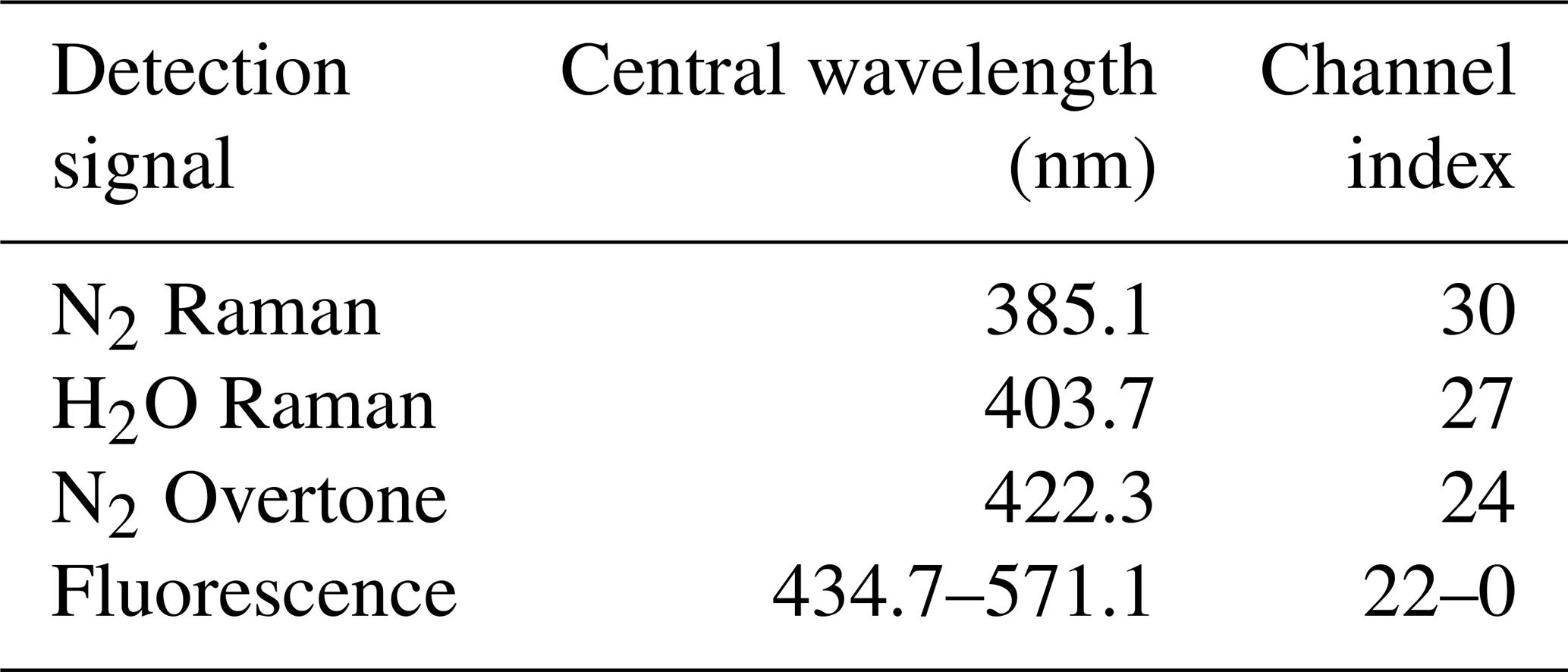
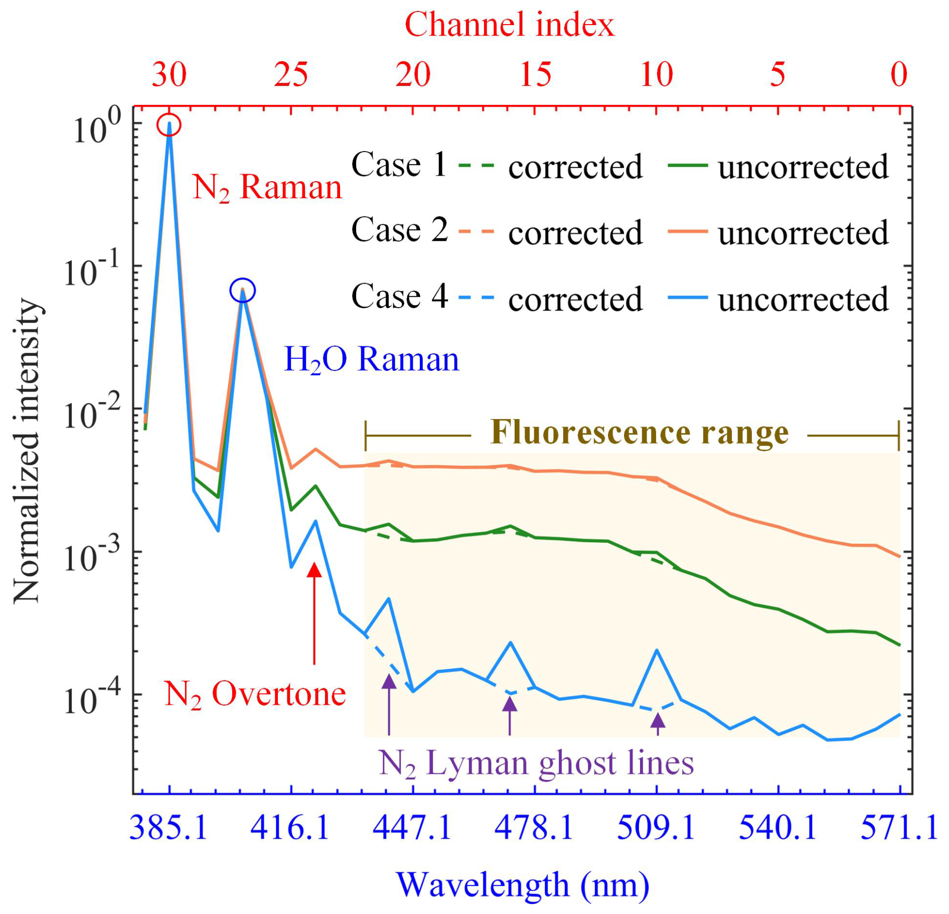
Figure 1 Mean fluorescence spectra for Cases 1 (1.0–1.8 km), 2 (1.0–1.8 km), and 4 (2.0–2.8 km) measured at the LIF lidar site. Line colors indicate the different cases. Solid lines show spectra before ghost-line correction and dashed lines show spectra after ghost-line correction (see legend). All the spectra are normalized by the N₂ Raman signal.

2.2 Satellite, radiosonde and ground-based observations

The Moderate-Resolution Imaging Spectroradiometer (MODIS) is a spaceborne multispectral sensor widely used in BBA studies (Shi et al., 2019; Yin, 2020). In this study, we utilized the MODIS Corrected Reflectance (True Color) imagery acquired on 16 April 2024, to visually overview fire activities in the ICP. We selected two sub-regions from the imagery to illustrate the spatial distribution of fire sources (Fig. 4a–b). To further quantify and identify fire events, we obtained the MODIS Collection 6.1 (C6.1) standard active fire product from NASA's Fire Information for Resource Management System (FIRMS) (Giglio et al., 2016). This dataset includes fire locations, fire radiative power (FRP), detection confidence, and fire types. For quality control, we used fire points that had confidence > 80 %, FRP > 100 MW, and were classified as type 0 (presumed vegetation fires).

To get the water vapor mixing ratio (WVMR) profiles, we used radiosonde data of five cities in South China downloaded from the University of Wyoming's website (https://weather.uwyo.edu/, last access: 20 May 2026); the location distributions are shown in Fig. 7a. To avoid cloud contamination in the radiosonde profiles, we discarded any level with relative humidity (RH) exceeding 95 %, following the approach of Zhou et al. (2025).

The AErosol RObotic NETwork (AERONET) (Holben et al., 1998) is a global ground-based aerosol monitoring program jointly established by NASA and PHOTONS (a European initiative coordinated by the University of Lille, the French National Centre for Space Studies, and the National Institute for Earth Sciences and Astronomy of CNRS). To support the identification of BBA transport events, we selected three AERONET sites near burning areas in the ICP (Chiang_Mai_Met_Sta, Doi_Ang_Khang, and Luang_Namtha); their geographic locations are marked as red triangles in Fig. 4e. Temporal variations in the aerosol optical depth at 500 nm (AOD@500 nm) provided auxiliary evidence for biomass burning plumes. We obtained air pollution data (including PM_2.5 and PM₁₀ concentrations) from the China National Environmental Monitoring Centre (CNEMC). To reduce localized variability and measurement noise, we averaged data from three monitoring stations near the LIF lidar site.

2.3 Reanalysis data and trajectory model

ERA5 (Hersbach et al., 2020) is the fifth-generation global climate reanalysis dataset from the European Centre for Medium-Range Weather Forecasts (ECMWF). In this study, we used ERA5 data to characterize temperature, geopotential, wind fields, and RH at different altitudes, providing essential meteorological context for our analysis. The Modern-Era Retrospective analysis for Research and Applications, Version 2 (MERRA-2) is a long-term global reanalysis developed by NASA's Global Modeling and Assimilation Office (GMAO). It assimilates satellite-based aerosol observations to represent interactions between aerosols and other physical processes in the climate system (Gelaro et al., 2017). In this study, we used hourly biomass burning OC emissions from the MERRA-2 tavg1_2d_adg_Nx hourly dataset with a spatial resolution of 0.625° × 0.5°.

The Hybrid Single-Particle Lagrangian Integrated Trajectory (HYSPLIT) model, developed by NOAA's Air Resources Laboratory, is widely used to analyze atmospheric transport, dispersion, air parcel trajectories, and pollutant transport pathways (Stein et al., 2015). In this study, we employed 78 h backward trajectory analysis using the HYSPLIT model, initialized at the LIF lidar site, aiming to identify the transport history and potential source regions of the observed fluorescent aerosol layer. The meteorological inputs were from the Global Data Assimilation System (GDAS).

3 LIF lidar data processing

3.1 Ghost line calibration

The calibration procedure was initially performed on the original fluorescence spectrum. Additionally, unavoidable imperfections in the diffraction grating can cause periodic spectral artifacts in fluorescence spectra, especially under weak fluorescence conditions. In our study, minor spurious peaks were found at Channels 21, 16, and 10 (Fig. 1). These peaks, known as Lyman ghosts (Tang et al., 2025a), were corrected based on their dependence on the primary wavelength (N₂ Raman signal; Channel 30, with a central wavelength of 385.1 nm) (Meggers and Kiess, 1922). In Fig. 1, the spectra are normalized by the N₂ Raman signal. For each case, both uncorrected and corrected curves are shown for direct comparison. To quantify ghost contributions and standardize correction across all spectral data, we selected three spectra with the lowest fluorescence intensity from three cases (where the N₂ Raman signal maintains sufficient intensity to ensure calibration reliability). One of them is the spectrum from Case 4 (2.0–2.8 km), which is shown in Fig. 1. For this spectrum, the three ghost-affected intervals (Channels 21, 16, and 10) were removed and reconstructed using linear interpolation, yielding a ghost-free reference spectrum (bottom blue dashed line in Fig. 1). The differences between the two blue curves at the three affected channels represent the characteristic ghost contribution for each channel. Ghost correction coefficients were then defined as these channel-specific differences divided by the corresponding N₂ Raman signal intensity from the same spectrum. The final channel-specific ghost correction coefficients were obtained by averaging the corresponding coefficients from the three reference spectra. All analyzed spectra were corrected using the same three coefficients (one per ghost-affected channel). During the correction, ghost contributions were estimated as the product of the N₂ Raman signal intensity and channel-specific coefficients, and subsequently subtracted from the original values to obtain the corrected spectra. Representative results for Cases 1 and 2 are shown in Fig. 1, where the dashed lines denote ghost-free spectra.

3.2 Retrieval of aerosol extinction and fluorescence backscatter coefficients

The aerosol extinction coefficient at distance z from the lidar is given by (Ansmann et al., 1990):

$$\begin{array}{}\text{(1)}& {\displaystyle }D=\mathrm{d}/\mathrm{d}z\left\{\ln \left[N_{\mathrm{R}}\left(z\right)/P_{\mathrm{R}}\left(z\right)z^{\mathrm{2}}\right]\right\}\text{(2)}& {\displaystyle }{\mathit{\alpha }}_{\mathrm{L}}^{\mathrm{aero}}\left(z\right)={\displaystyle \frac{D-{\mathit{\alpha }}_{\mathrm{L}}^{\mathrm{mole}}\left(z\right)-{\mathit{\alpha }}_{\mathrm{R}}^{\mathrm{mole}}\left(z\right)}{\mathrm{1}+{\left({\mathit{\lambda }}_{\mathrm{L}}/{\mathit{\lambda }}_{\mathrm{R}}\right)}^k}}\end{array}$$

where the superscripts “aero” and “mole” indicate quantities related to aerosols and molecules, respectively. The subscripts “L” and “R” correspond to elastic and N₂ Raman channels. ${\mathit{\alpha }}_{\mathrm{R}}^{\mathrm{mole}}$ and ${\mathit{\alpha }}_{\mathrm{L}}^{\mathrm{mole}}$ are the molecular extinction coefficients in elastic and N₂ Raman channels, calculated following Platt et al. (2012). N_R is the nitrogen number density, which is calculated from temperature and pressure values obtained from the ERA5 reanalysis dataset. λ_L and λ_R denote the elastic wavelength and the N₂ Raman channel central wavelength (385.1 nm), respectively. The Ångström exponent k is assumed to be 1 (Ansmann et al., 1992a).

The fluorescence backscatter coefficient is given by (Veselovskii et al., 2020):

$$\begin{array}{}\text{(3)}& {\mathit{\beta }}_{\mathrm{F}}={\displaystyle \frac{C_{\mathrm{R}}}{C_{\mathrm{F}}}}{\displaystyle \frac{P_{\mathrm{F}}}{P_{\mathrm{R}}}}{\displaystyle \frac{T_{\mathrm{R}}}{T_{\mathrm{F}}}}{N}_{\mathrm{R}}{\mathit{\sigma }}_{\mathrm{R}}\end{array}$$

where P_R and P_F are the lidar signals from the N₂ Raman and fluorescence (Channels 22–0, with central wavelengths of 434.7–571.1 nm) channels, respectively. σ_R is the N₂ Raman differential backscatter cross section at 355 nm (Venable et al., 2011). T_R and T_F are the atmospheric transmittance for the N₂ Raman and fluorescence channels, respectively. C_R and C_F are system constants for the N₂ Raman and fluorescence channels, respectively. Similarly, the water vapor Raman backscatter coefficient ${\mathit{\beta }}_{{\mathrm{H}}_{\mathrm{2}}\mathrm{O}}$ is derived by replacing the fluorescence channels with the water vapor Raman channel (Channel 27, with a central wavelength of 403.7 nm). Unlike single-channel fluorescence systems, our LIF lidar employs 23 fluorescence channels. Accordingly, the fluorescence backscatter coefficient β_F is obtained by summing contributions from all individual channels. For comparison, β_F is then normalized by the fluorescence spectral wavelength range Δλ to yield the spectral fluorescence backscatter coefficient:

$$\begin{array}{}\text{(4)}& {\stackrel{\mathrm{‾}}{\mathit{\beta }}}_{\mathrm{F}}={\displaystyle \frac{{\mathit{\beta }}_{\mathrm{F}}}{\mathrm{\Delta }\mathit{\lambda }}}\end{array}$$

4 Results

4.1 Vertical profiles observed by LIF lidar

Time-height profiles of four representative nighttime cases observed in 2024 are shown in Fig. 2. All observations were conducted at night to avoid strong solar background interference during the daytime. Four cases are included: Case 1 (19 April, 23:19–20 April, 00:05), when a distinct fluorescence layer was observed (Fig. 2c); Case 2 (11 May, 01:41–02:37); Case 3 (18 May, 21:43–23:29); and Case 4 (23 May, 21:27–23:08). All times are in local time (UTC+8), with the time axis labeled at 20 min intervals. The vertical white lines separate individual cases. Figure 2a–c show the range-corrected signal (RCS) of different detection channels, while Fig. 2d–f present retrieved parameters derived via the methods described in Sect. 3.2. The detection lower limit is within 800 m, which defines the starting altitude of all subplots. The N₂ Raman signal (Fig. 2a) decays more slowly in Case 4 than in the other three cases, likely due to the lower aerosol loading (Figs. 2d and A1a). The fluorescence intensity is also relatively weak in Case 4 (Figs. 2c, f and 3), making this case ideal for calibrating the Lyman ghost lines. In Cases 1, 3, and 4 (3–4 km), we observed abrupt enhancements in ${\mathit{\alpha }}_{\mathrm{L}}^{\mathrm{aero}}\left(z\right)$ (Fig. 2d), indicating the presence of clouds (Sugimoto et al., 2012). In Case 3, the fluorescence layer ascends to ∼ 3 km due to the vertical mixing (Fig. 2f). This upward shift is further evident in Fig. 3, where the averaged ${\stackrel{\mathrm{‾}}{\mathit{\beta }}}_{\mathrm{F}}$ (0.8–1.4 km) decays rapidly in all cases except Case 3.

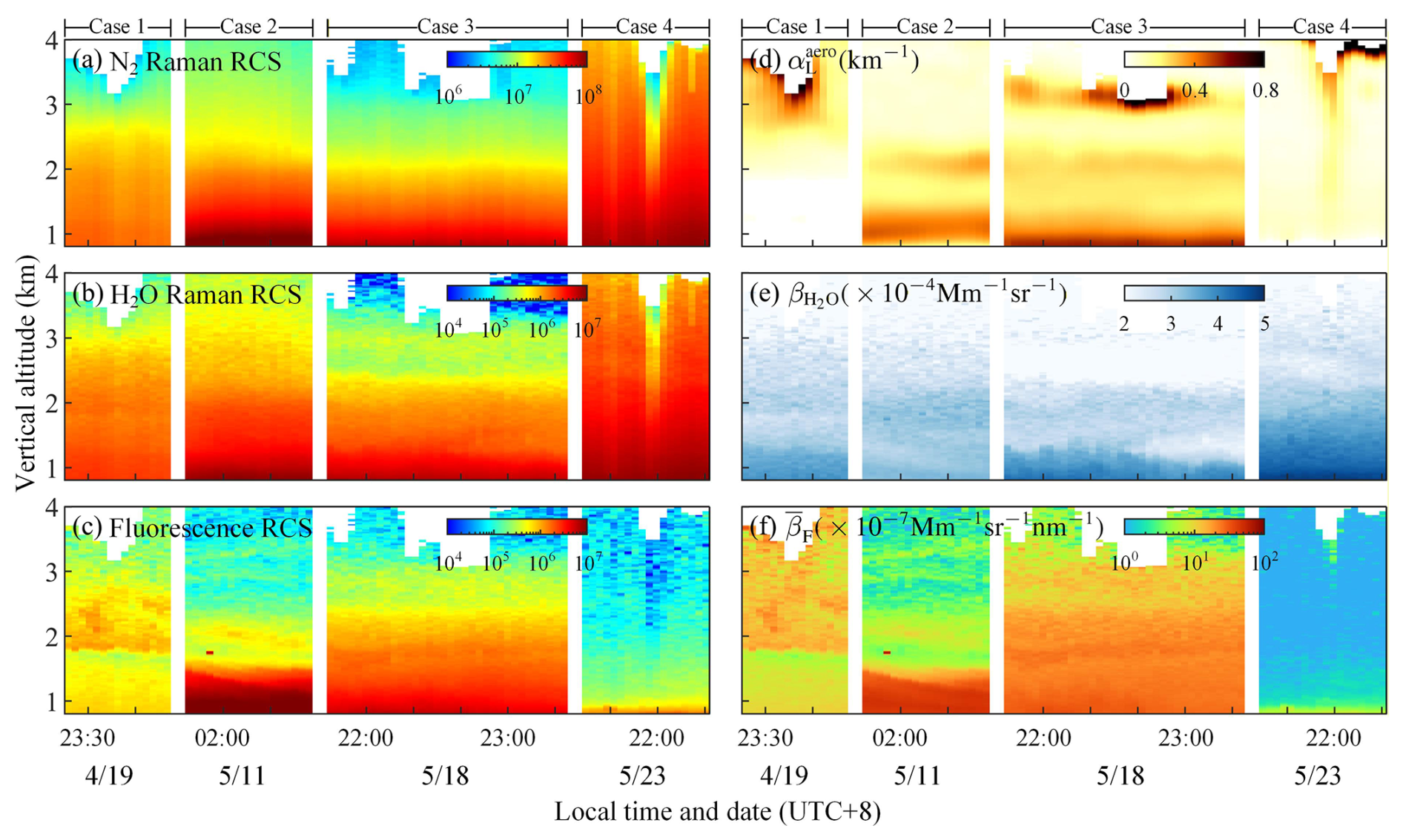
Figure 2 Time-height profiles for the four cases at the LIF lidar site during 19 April–23 May 2024 (UTC+8). (a–c) The range-corrected signal (RCS) from the respective detection channels (as defined in Table 1). (d–f) Retrieved quantities for panels (a)–(c), respectively; retrieval methods are described in Sect. 3.2.

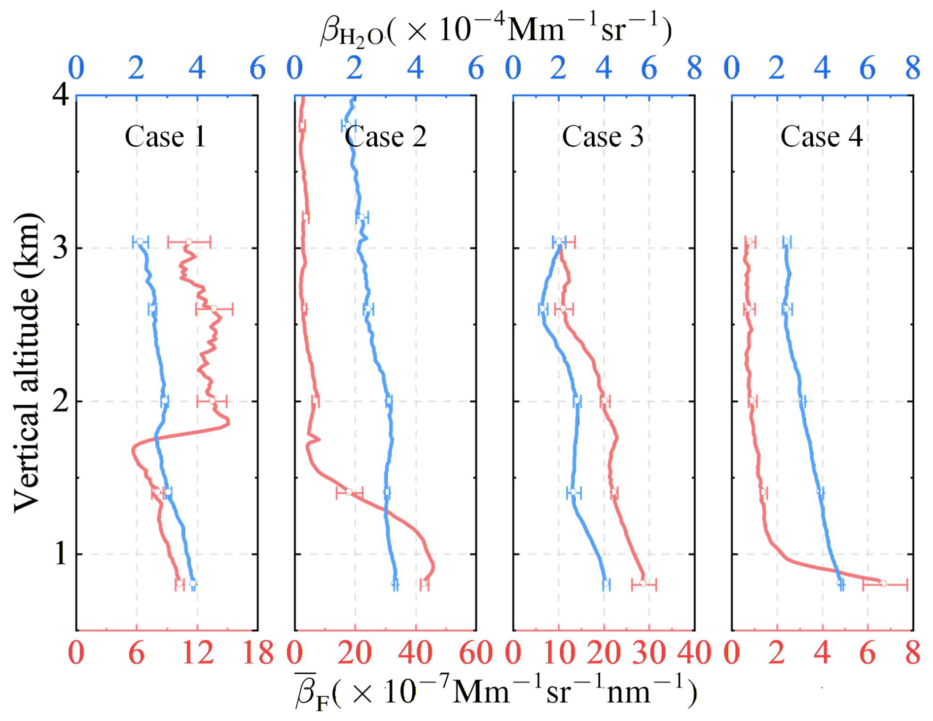
Figure 3 Mean vertical profiles of ${\mathit{\beta }}_{{\mathrm{H}}_{\mathrm{2}}\mathrm{O}}$ (blue lines) and ${\stackrel{\mathrm{‾}}{\mathit{\beta }}}_{\mathrm{F}}$ (red lines) for the four cases at the LIF lidar site. Error bars indicate ±1 standard deviation across the profile samples.

Figure A1 presents the relationships among averaged ${\stackrel{\mathrm{‾}}{\mathit{\beta }}}_{\mathrm{F}}$, ${\mathit{\alpha }}_{\mathrm{L}}^{\mathrm{aero}}$ (0.8–1.4 km), surface RH, and surface PM concentrations. In Cases 1 and 4, RH remains close to saturation following preceding precipitation, favoring efficient wet deposition and resulting in reduced aerosol loading. Consequently, lower ${\mathit{\alpha }}_{\mathrm{L}}^{\mathrm{aero}}$ (< 0.1 km⁻¹) are observed compared to Cases 2 and 3 (> 0.3 km⁻¹), which qualitatively agrees with the observed PM concentration differences. The slightly negative layer-averaged ${\mathit{\alpha }}_{\mathrm{L}}^{\mathrm{aero}}$ in Case 1 can be attributed to retrieval uncertainties under very clean conditions, a behavior also reported in previous studies (Ansmann et al., 1992b; Hu et al., 2025). In particular, hygroscopic growth under elevated RH can enhance aerosol optical extinction by modifying particle size and refractive index (Ansmann et al., 1992a; Haarig et al., 2025). This effect likely contributes to the slightly higher ${\mathit{\alpha }}_{\mathrm{L}}^{\mathrm{aero}}$ in Case 2 compared to Case 3 (RH ≈ 89.2 % versus ≈ 83.6 %). In contrast to aerosol extinction, fluorescence signals are expected to be much less affected by ambient humidity and hygroscopic growth. Under the assumption of minimal water-induced fluorescence quenching (Veselovskii et al., 2025b), negligible hygroscopic effects on aerosol fluorescence, and unchanged aerosol mixing state, ${\stackrel{\mathrm{‾}}{\mathit{\beta }}}_{\mathrm{F}}$ can be regarded as a reliable proxy for dry aerosol material concentrations (Miri et al., 2024), which is consistent with the dry-state nature of the measured PM mass concentrations. However, the relative magnitudes of ${\stackrel{\mathrm{‾}}{\mathit{\beta }}}_{\mathrm{F}}$ in Cases 2 and 3 still exhibit an opposite ordering compared to PM concentrations, indicating that aerosol fluorescence does not scale linearly with bulk particulate mass. This discrepancy reflects the combined influence of fluorescent particle types and concentrations, rather than particle mass alone (Reichardt, 2014).

In Case 1, a distinct fluorescent layer (enhanced ${\stackrel{\mathrm{‾}}{\mathit{\beta }}}_{\mathrm{F}}$) accompanied by enhanced water vapor was observed at ∼ 1.8 km despite relatively low ${\mathit{\alpha }}_{\mathrm{L}}^{\mathrm{aero}}$ (Figs. 2c, e, f, and 3). This enhancement is not observed in the other three cases (Fig. 3). To better constrain the aerosol source in Case 1 (1.8–2.4 km), HYSPLIT backward trajectory analysis was performed in Sect. 4.2.

4.2 Source attribution of the fluorescent layer in Case 1

HYSPLIT backward trajectories for Case 1 indicate that the air mass linked to the fluorescent layer originated from the ICP during 16–18 April 2024 (Fig. 4d). This event can be divided into three stages: local biomass burning, vertical lifting, and long-range transport. MODIS true-color imagery for 16–17 April (Fig. 4a–b) reveals multiple fire points, with near-surface plume orientations consistent with winds blowing toward the northeast (Fig. 4f–g). Two source regions with the most intense fire activity are highlighted by black boxes in Fig. 4d–g (these boxes correspond to the areas as in Fig. 4a–b). MODIS C6.1 fire products also identify numerous low-intensity vegetation fire pixels within these regions (Fig. 4d), while the MERRA-2 emission fields indicate elevated OC emissions coincident with these suspected sources (Fig. 4f–g). Additionally, the 10 m wind barbs align with the plume directions visible in the satellite imagery. As shown in Fig. 5, AOD@500 nm at three AERONET stations (locations marked as red triangles in Fig. 4e) increased during the period. The BBA then underwent vertical lifting to the 2–3 km altitude range (Fig. 4c). During the pre-monsoon season, frequent small-scale cumulus convection can transport pollutants above 3 km – an optimal altitude for long-range transport (Shan et al., 2016). For our case, a similar phenomenon was visible in Fig. 4a–b. Additionally, the higher terrain (Fig. 4d) also provides favorable conditions for BBA uplift. Thereafter, the BBA were rapidly transported by the southwest summer monsoon (Fig. 4d) to altitudes above our LIF lidar site, where a fluorescent layer was observed. On the contrary, HYSPLIT backward trajectory analysis with a starting altitude of 1 km show that the low-altitude fluorescence was not affected by the transported BBA (Fig. B1).

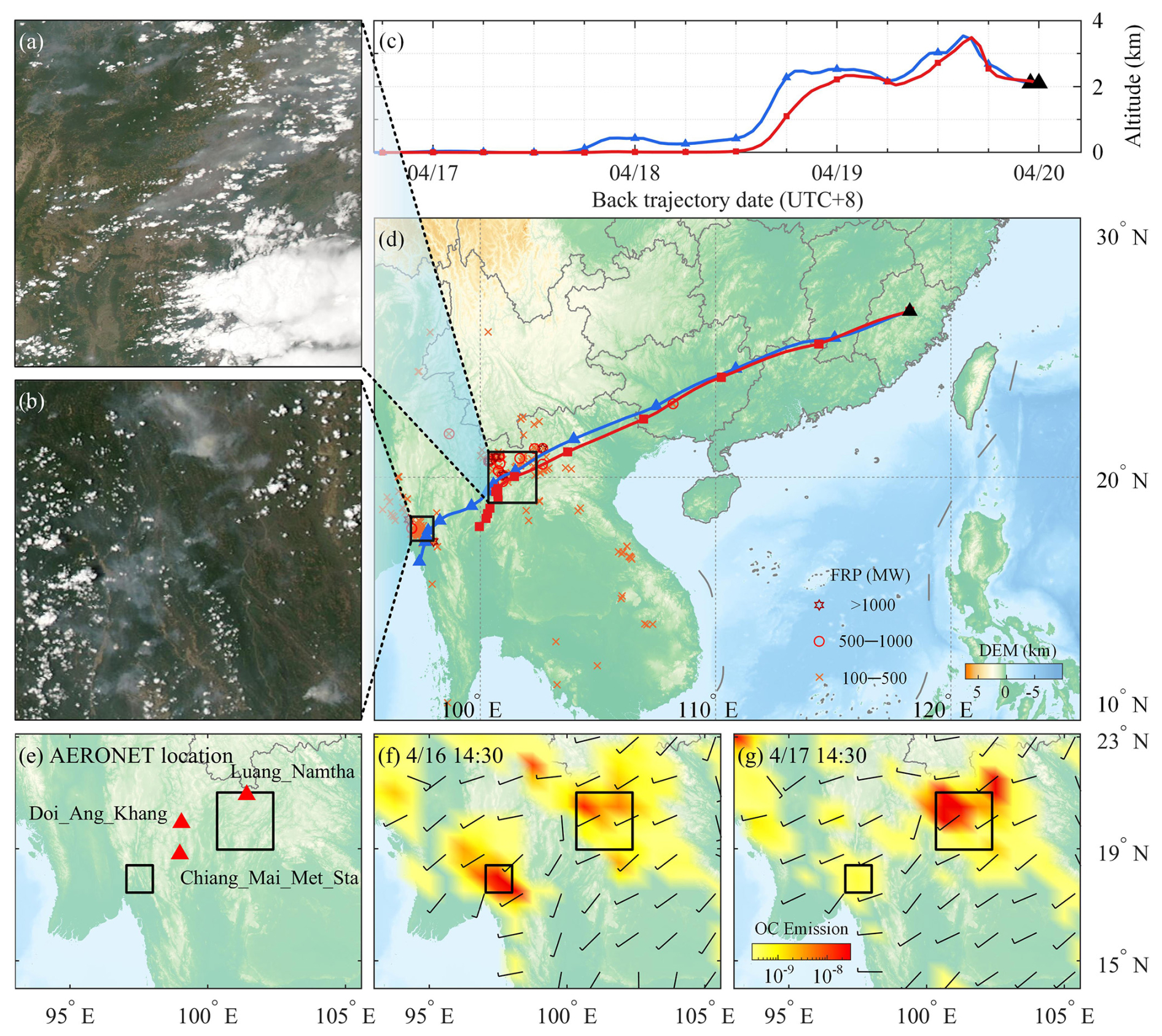
Figure 4 Imagery, trajectory analysis and modeled biomass burning emissions for Case 1. (a–b) MODIS (Aqua) true-color images acquired on 16 April 2024 (UTC), sourced from NASA Worldview (https://worldview.earthdata.nasa.gov/, last access: 20 May 2026), showing smoke plumes originating from multiple fire points (areas highlighted by black boxes in panels d–g). (c) Vertical variation of air mass altitude from HYSPLIT backward trajectories (starting altitude: 2.1 km). (d) Horizontal (longitude-latitude) HYSPLIT backward trajectories overlaid on presumed vegetation fire locations; marker colors and shapes indicate FRP levels, and the underlying digital elevation model (DEM) highlights topography (the black triangle denotes the LIF lidar site). (e) Locations of the AERONET stations (red triangles) used in Fig. 5. (f–g) MERRA-2 biomass burning organic carbon (OC) emissions (kg m⁻² s⁻¹) for two temporal conditions, plotted with background 10 m wind fields.

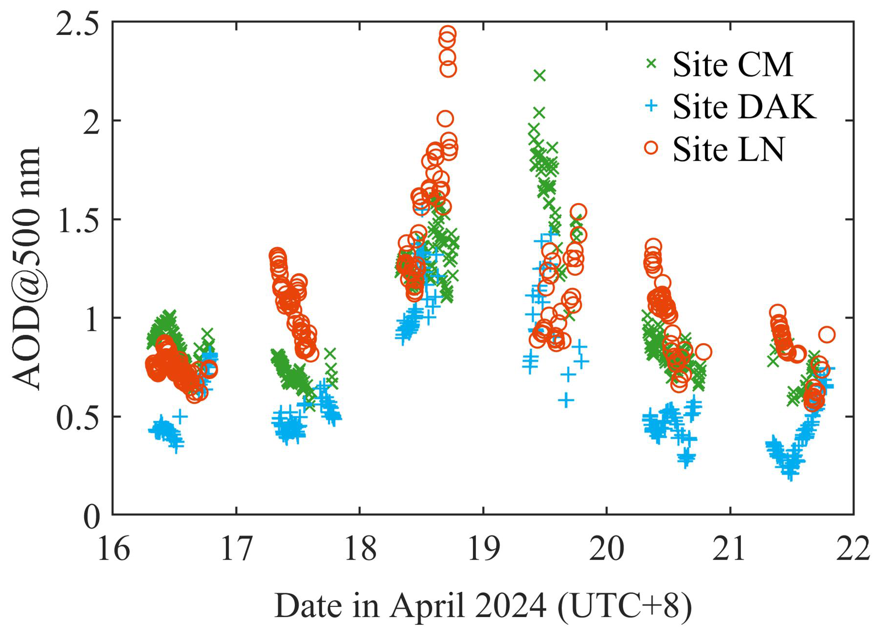
Figure 5 Aerosol optical depth at 500 nm (AOD@500 nm) retrieved from three AERONET sites during 16–22 April 2024. Marker colors and shapes indicate the stations: CM represents Chiang_Mai_Met_Sta, DAK represents Doi_Ang_Khang, and LN represents Luang_Namtha (locations shown in Fig. 4e, red triangles).

4.3 Spectral fluorescence capacity estimation

To further analyze the fluorescence characterization, we use quantitative analyses of the spectral fluorescence capacity $G_{\mathrm{F}}=\frac{{\stackrel{\mathrm{‾}}{\mathit{\beta }}}_{\mathrm{F}}}{{\mathit{\beta }}_{\mathrm{L}}}$, where ${\stackrel{\mathrm{‾}}{\mathit{\beta }}}_{\mathrm{F}}$ is the spectral fluorescence backscatter coefficient and β_L is the elastic backscatter coefficient (Reichardt, 2014; Veselovskii et al., 2022b). As β_L was not directly available in this study, we estimated ${\widehat{G}}_{\mathrm{F}}=\frac{{\stackrel{\mathrm{‾}}{\mathit{\beta }}}_{\mathrm{F}}}{{\mathit{\alpha }}_{\mathrm{L}}^{\mathrm{aero}}}\cdot S$ using a typical lidar ratio S≈55 sr for aged smoke (Ansmann et al., 2021). To enable direct comparability with the fluorescence wavelength range (444–488 nm) from Gast et al. (2025), we selected Channels 20–14 (444–487.4 nm) for ${\widehat{G}}_{\mathrm{F}}$ estimation. ${\widehat{G}}_{\mathrm{F}}$ values are provided in Table 2, excluding Case 1 (0.8–1.4 nm): negative ${\mathit{\alpha }}_{\mathrm{L}}^{\mathrm{aero}}$ results in negative ${\widehat{G}}_{\mathrm{F}}$, which is thus omitted. Table 2 presents the highest ${\widehat{G}}_{\mathrm{F}}$ for Case 1 (1.8–2.4 km) $\approx \mathrm{1.6}\times {\mathrm{10}}^{-\mathrm{6}}$ nm⁻¹, which is close to the lower bound of the G_F range ($\mathrm{1.5}\times {\mathrm{10}}^{-\mathrm{6}}$–$\mathrm{13}\times {\mathrm{10}}^{-\mathrm{6}}$ nm⁻¹) reported for smoke observed in Germany (Gast et al., 2025). Notably, ${\widehat{G}}_{\mathrm{F}}$ for Case 1 (1.8–2.4 km) is at least twice as high as those retrieved from the other layers, indicating relatively enhanced fluorescence efficiency in this layer. The characteristics of the fluorescent layer are further examined through analysis of the fluorescence spectra in Sect. 4.4.

Table 2 Estimates of layer-averaged spectral fluorescence capacity $\left({\widehat{G}}_{\mathrm{F}}=\frac{{\stackrel{\mathrm{‾}}{\mathit{\beta }}}_{\mathrm{F}}}{{\mathit{\alpha }}_{\mathrm{L}}^{\mathrm{aero}}}\cdot S\right)$, computed over the fluorescence spectral range 444–487.4 nm (Channels 20–14). A lidar ratio S of 55 sr (typical for aged smoke) is assumed (Ansmann et al., 2021).

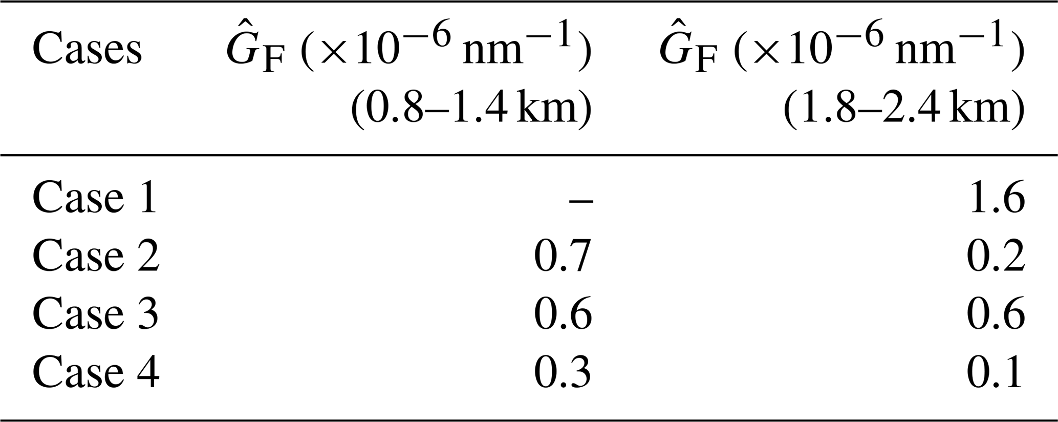
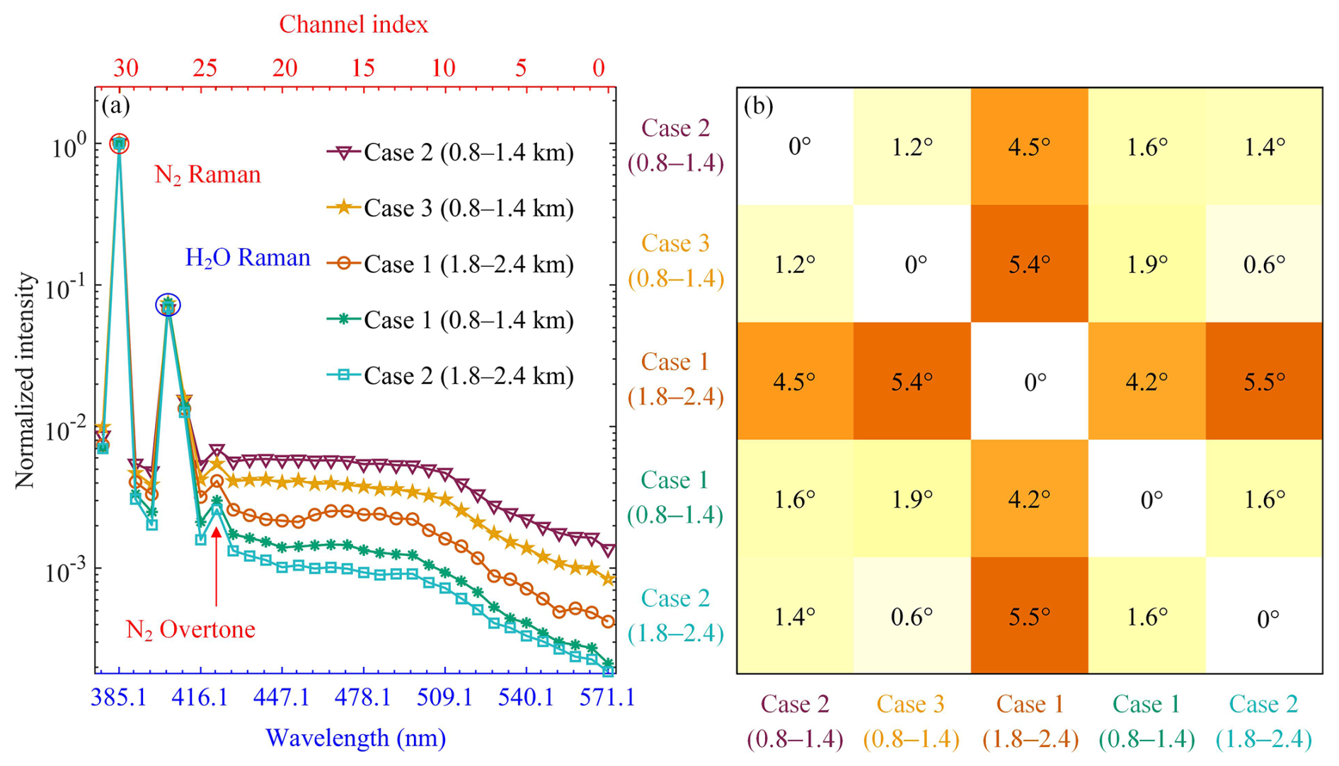
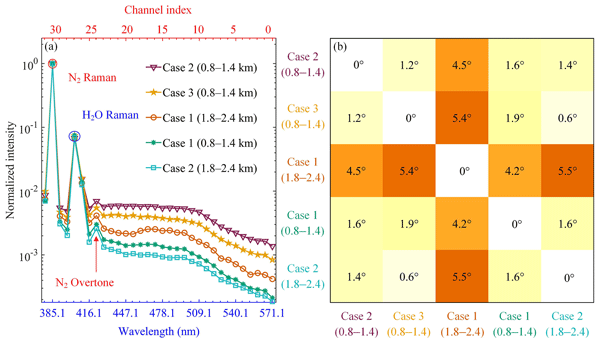
Figure 6 (a) Mean fluorescence spectra (normalized by N₂ Raman signal) derived from 600 m-thick layers for Cases 1–3. Line colors and marker shapes denote the different cases and layer altitudes (see legend). (b) SAM angle matrix for the five selected spectra (Channels 20–14, 444–487.4 nm). A SAM angle of 0° indicates identical spectral shapes, with larger angles corresponding to greater dissimilarity.

4.4 Fluorescence spectra

As shown in Fig. 6a, mean fluorescence spectra from multiple 600 m thick layers are normalized to the N₂ Raman signal. The maximum fluorescence intensity is more than two orders of magnitude lower than that of the N₂ Raman signal. To quantitatively analyze the spectral similarity, we adopted the spectral angle mapping (SAM) analysis (Farsund et al., 2010) using Channels 20–14 (444–487.4 nm) from the fluorescence spectra. This algorithm quantifies spectral similarity by treating spectra as vectors and calculating the vector angle, ranging from 0° (identical spectral shapes) to 90° (completely distinct spectral shapes). Figure 6b shows the SAM angle matrix for the selected spectra in Fig. 6a. The low SAM angle (≈ 1.2°) between Cases 2 and 3 (0.8–1.4 km) indicates high spectral similarity. Both spectra exhibit decreasing intensity with increasing wavelength, consistent with reported urban aerosol spectra in the boundary layer (Veselovskii et al., 2025a).The spectrum of Case 1 (1.8–2.4 km) is distinct from other spectra (Fig. 6a), with quantitative support from spectral angle mapping (SAM) analysis (Fig. 6b): the SAM angle between Case 1 (1.8–2.4 km) and Cases 2 and 3 (0.8–1.4 km) is ∼ 5.0°, notably larger than the SAM angle (≈ 1.2°) between Cases 2 and 3 (0.8–1.4 km) themselves. Additionally, SAM angles between Case 1 (1.8–2.4 km) and Case 1 (0.8–1.4 km) as well as between Case 1 (1.8–2.4 km) and Case 2 (1.8–2.4 km) both exceed 4°, further confirming the spectral dissimilarity.

5 Discussion

Considering the distinct ${\stackrel{\mathrm{‾}}{\mathit{\beta }}}_{\mathrm{F}}$ layer (Fig. 2f), HYSPLIT backward trajectory analysis (Fig. 4d), the highest ${\widehat{G}}_{\mathrm{F}}$ ($\approx \mathrm{1.6}\times {\mathrm{10}}^{-\mathrm{6}}$ nm⁻¹; Table 2) and the unique fluorescence spectral shape (Fig. 6a–b), these lines of evidence support that BBA transported from the ICP was a major contributor to the fluorescent layer observed in Case 1 (1.8–2.4 km). For the fluorescence spectra of Cases 2 and 3 (0.8–1.4 km), considering the spectral features in Sect. 4.2 with the low ${\widehat{G}}_{\mathrm{F}}$ ($\le \mathrm{1}\times {\mathrm{10}}^{-\mathrm{6}}$ nm⁻¹; Table 2) and the higher averaged ${\mathit{\alpha }}_{\mathrm{L}}^{\mathrm{aero}}$ (0.8–1.4 km) in Cases 2 and 3 compared to Cases 1 and 4 (linked with PM concentration trends; Fig. A1), our results suggest that the fluorescence of Cases 2 and 3 (0.8–1.4 km) observed at our LIF lidar site was likely attributable to urban aerosol. Regarding potential biogenic interference, although local dominant tree species (e.g., pines) may release pollen in May, pollen is unlikely to be the dominant contributor to the fluorescence signal in Cases 2 and 3 (0.8–1.4 km). This is evidenced by the absence of distinct characteristic peaks in the fluorescence spectra (Saito et al., 2018) and the low ${\widehat{G}}_{\mathrm{F}}$.

The Asian summer monsoon brings substantial rainfall to the region, while the pre-monsoon season (March–April) is typically dry across the ICP. During this period, frequent biomass burning events (predominantly forest fires and agricultural burnings) lead to seasonal peaks in BBA loadings (Gautam et al., 2013; Shi and Yamaguchi, 2014). Fire activity peaks in March but declines sharply by late April (Huang et al., 2016). MODIS FRP data indicate that over 84 % of fire points had FRP < 500 MW (with only a few high-intensity points), while MERRA-2 data show a maximum OC emission rate of $\mathrm{1.5}\times {\mathrm{10}}^{-\mathrm{8}}$ kg m⁻² s⁻¹. The detected fluorescent layer was relatively weak, with a fluorescence signal intensity more than two orders of magnitude lower than the N₂ Raman signal intensity. The maximum ${\stackrel{\mathrm{‾}}{\mathit{\beta }}}_{\mathrm{F}}\approx \mathrm{0.16}\times {\mathrm{10}}^{-\mathrm{5}}$ Mm⁻¹ sr⁻¹ nm⁻¹ observed in Case 1 (1.8–2.4 km) lies at the lower end of the range of ${\stackrel{\mathrm{‾}}{\mathit{\beta }}}_{\mathrm{F}}$ values reported for BBA in France (Hu et al., 2022), Germany (Gast et al., 2025; Reichardt et al., 2025), and Russia (Veselovskii et al., 2025a). Consistent with the high sensitivity of LIF lidar reported in previous studies (Gast et al., 2025; Reichardt et al., 2025), our results show that weak, long-range transported BBA from the ICP can be observed over South China during periods of relatively weak fire activity (e.g., late April).

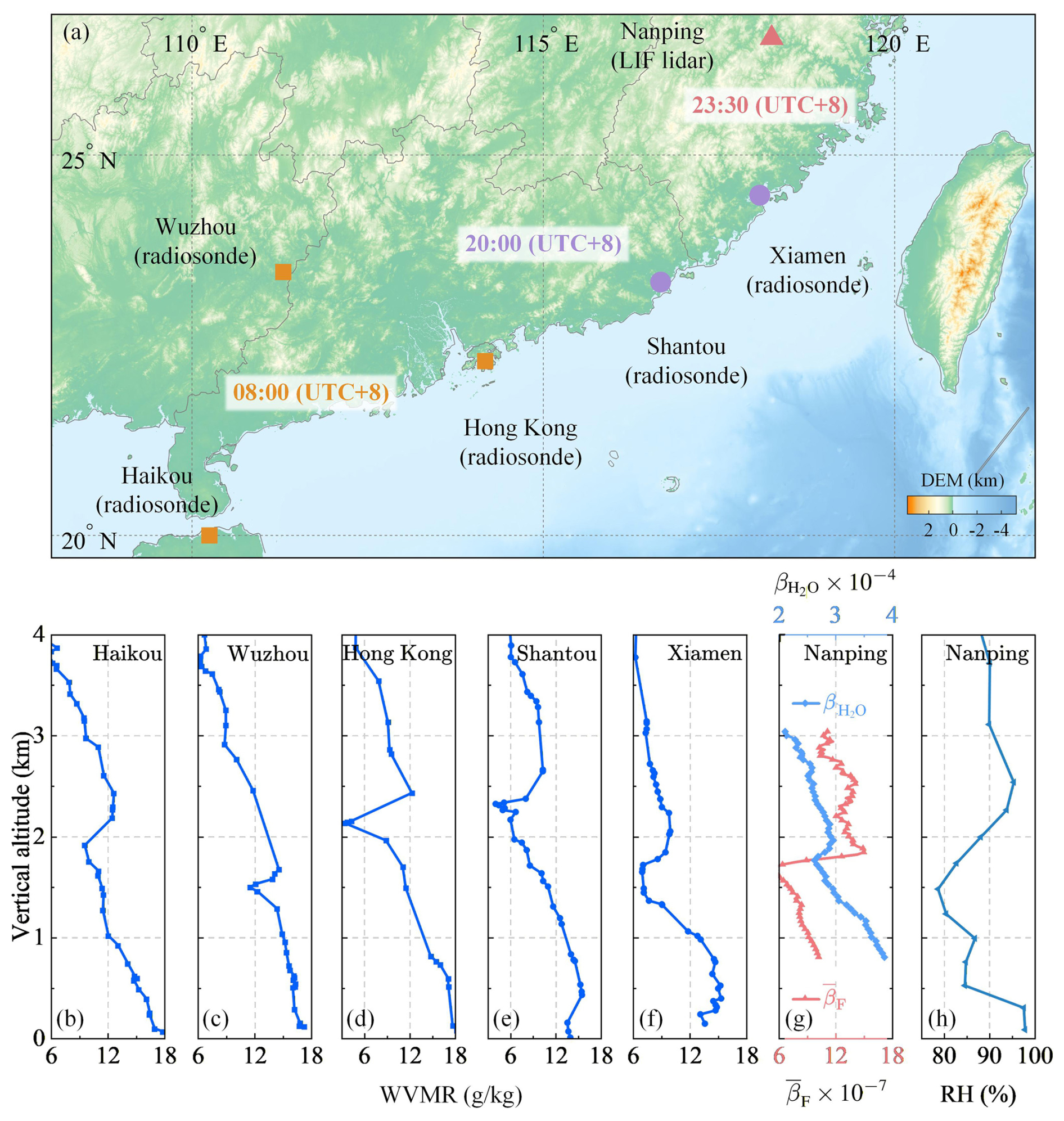
Figure 7 Radiosonde, LIF lidar, and reanalysis profiles for 19 April 2024 (UTC+8), Case 1. (a) Map overview of radiosonde launch sites and the LIF lidar site; marker colors and shapes indicate acquisition time; the LIF lidar measurement period is 19 April 2024, 23:19–20 April 00:05 (UTC+8). (b–f) Water vapor mixing ratio (WVMR) profiles from radiosonde measurements. (g) Water vapor Raman backscatter coefficient ${\mathit{\beta }}_{{\mathrm{H}}_{\mathrm{2}}\mathrm{O}}$ (Mm⁻¹ sr⁻¹) and spectral fluorescence backscatter coefficient ${\stackrel{\mathrm{‾}}{\mathit{\beta }}}_{\mathrm{F}}$ (Mm⁻¹ sr⁻¹ nm⁻¹) profiles. (h) ERA5 RH profile for Nanping at 19 April 2024, 23:00 (UTC+8).

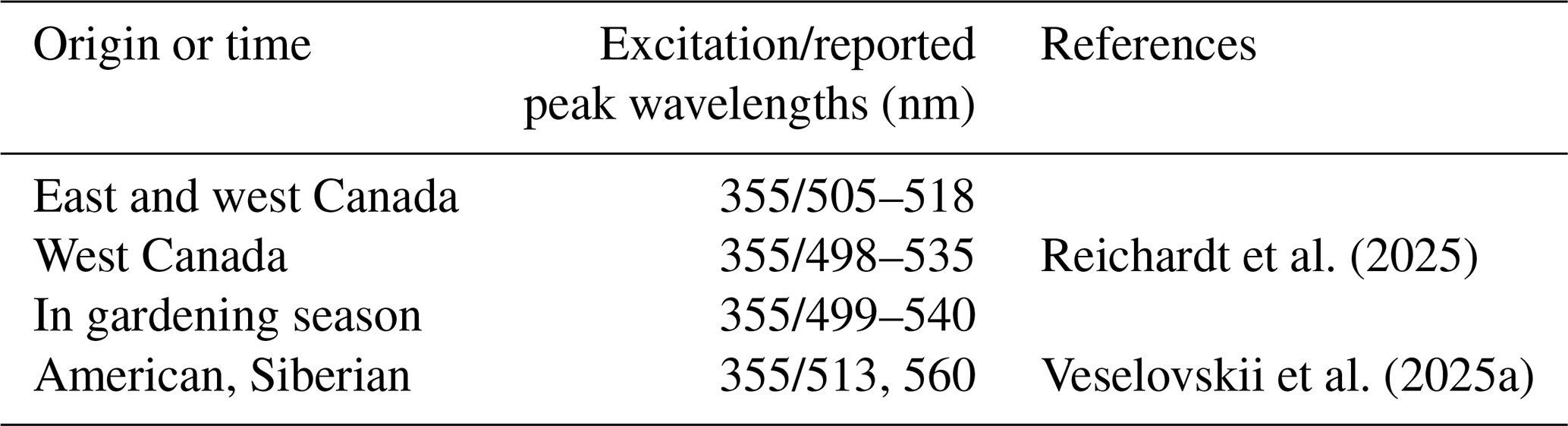
For the spectrum of Case 1 (1.8–2.4 km), the relatively weak peak intensity is likely attributable to the overall low fluorescence signal intensity (which is over two orders of magnitude lower than the N₂ Raman signal) and mixing with urban aerosol due to the long-range transport, while the peak wavelength discrepancy relative to previous studies is likely due to distinct fire sources. Biomass burning emits complex carbonaceous aerosols, which undergo further chemical transformations during atmospheric transport and result in more diverse compositions (Hodshire et al., 2019; Wang et al., 2019). Many components in BBA, such as polycyclic aromatic hydrocarbons (PAHs) and humic-like substances (HULIS), can produce fluorescence under UV excitation (Pöhlker et al., 2012; Yue et al., 2022). As shown in Fig. 6a, Case 1 (1.8–2.4 km) exhibited a spectral shoulder which begins at Channel 18 (central wavelength is 459.5 nm), suggesting the presence of fluorophores. As summarized in Table C1, fluorescence peaks in the 440–480 nm range have been reported for certain PAHs and HULIS under ∼ 355 nm excitation, which are similar to our observed spectral feature. In contrast, previous LIF lidar observations in Europe exhibited BBA fluorescence peak wavelengths approximately between 498 and 560 nm (Table C2), highlighting the influence of source characteristics and atmospheric processing on spectral signatures. Via vertical mixing, such transported BBA may influence the near-surface atmosphere (Dajuma et al., 2020). Future observations combining LIF lidar with in-situ instrumentation such as the Wideband Integrated Bioaerosol Sensor (WIBS), which also operates on LIF principles (Tang et al., 2022), would facilitate a more in-depth investigation of the near-surface impacts exerted by transported BBA. Combined LIF lidar and WIBS measurements have recently been reported (Gidarakou et al., 2026).

To further investigate BBA transport processes, we analyzed radiosonde observations from multiple sites in South China (Fig. 7a), with colors representing different observation times corresponding to the BBA transport period (Fig. 4d, the “long-range transport” stage). In Fig. 7g, the ${\stackrel{\mathrm{‾}}{\mathit{\beta }}}_{\mathrm{F}}$ shows a marked increase at 1.8 km, coinciding with enhanced ${\mathit{\beta }}_{{\mathrm{H}}_{\mathrm{2}}\mathrm{O}}$ at Nanping. Previous studies have suggested that fluorescence interference in water vapor Raman channels (Chouza et al., 2022; Liu et al., 2022) may contribute to an enhancement in ${\mathit{\beta }}_{{\mathrm{H}}_{\mathrm{2}}\mathrm{O}}$. However, in our measurements, the fluorescence signal is approximately one order of magnitude lower than the water vapor Raman signal (Fig. 6a). As a sensitivity test, we subtracted the signal from a nearby fluorescence channel (Channel 22) from the water vapor Raman channel and found that the enhanced ${\mathit{\beta }}_{{\mathrm{H}}_{\mathrm{2}}\mathrm{O}}$ layer persists, suggesting that fluorescence interference is limited. In addition, the ERA5 RH profile (Fig. 7h) shows a distinct high-humidity layer at the same altitude, which is consistent with the presence of a real moisture layer. As shown in Fig. 4d, HYSPLIT backward trajectories indicate that the observed BBA layer originated from fire sources near coastal regions and was transported inland by onshore flow, which suggests possible entrainment of marine aerosols (such as sea salt) (Dang et al., 2022). Furthermore, radiosonde data (Fig. 7b–f) reveal that the BBA was co-transported with water vapor, a feature consistent with previous lidar and in-situ observations (Kim et al., 2009; Fadnavis et al., 2013; Pistone et al., 2021; Chavan et al., 2021; Hu et al., 2022; Rubin et al., 2023; Pistone et al., 2024). Such humid, sea salt containing conditions could enhance sunlight driven reactions, accelerating secondary sulfate formation and thereby exerting important environmental impacts (Tang et al., 2023, 2025b).

6 Conclusion

In this study, we report LIF lidar observations at Nanping, South China during April–May, 2024. A distinct fluorescent layer was observed, exhibiting unique spectral characteristics and an estimated fluorescence capacity (${\widehat{G}}_{\mathrm{F}}\approx \mathrm{1.6}\times {\mathrm{10}}^{-\mathrm{6}}$ nm⁻¹). HYSPLIT backward trajectory analysis indicates that this layer originated from low-intensity fire points in the ICP. These lines of evidence support that the BBA transported from the ICP was a major contributor to the fluorescent layer. Consistent with the high sensitivity of LIF lidar reported in Europe (Gast et al., 2025; Reichardt et al., 2025), these results show that LIF lidar can detect faint BBA fluorescence signals from relatively weak fires in Asia. Fluorescence spectral analysis reveals a peak similar to those reported in previous in-situ studies of certain hazardous organics. However, the peak wavelengths of fluorescence spectra differ from previous LIF lidar studies, suggesting compositional variability linked to source types or aging processes. Notably, co-transport of water vapor with the BBA was also observed, which may enhance aerosol processing and increase impacts in downwind regions.

March marks the peak of seasonal biomass burning across the ICP, with widespread agricultural burning (for planting preparation) and forest fires (Gautam et al., 2013; Huang et al., 2016). As South China lies downwind of the ICP, it provides a favorable setting for long-term LIF lidar observations of transported BBA across different stages of the burning season. To improve quantitative aerosol classification, a LIF lidar system that integrates elastic scattering, depolarization, and fluorescence detection is under development. It will enable direct retrieval of spectral fluorescence capacity G_F (Reichardt, 2014) and depolarization ratio – key parameters for refining aerosol type differentiation (Veselovskii et al., 2022b) and gaining deeper insights into regional BBA characteristics.

Appendix A: Meteorological parameters and cases comparison

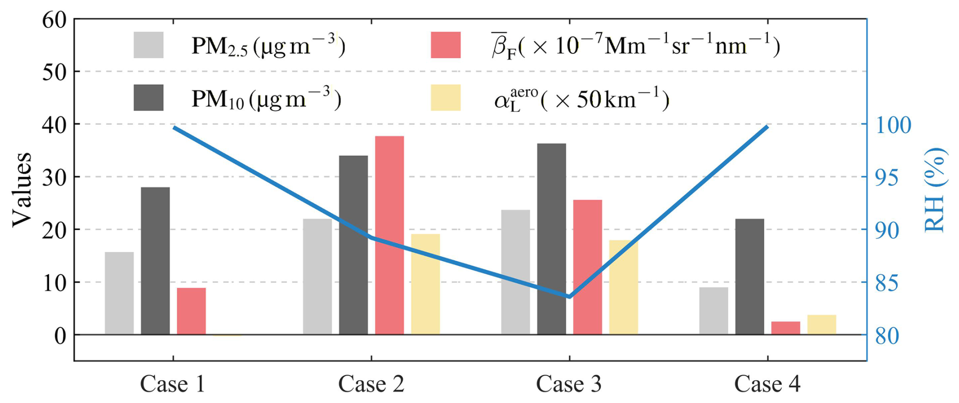
Figure A1 Comparison of key parameters: averaged ${\stackrel{\mathrm{‾}}{\mathit{\beta }}}_{\mathrm{F}}$, ${\mathit{\alpha }}_{\mathrm{L}}^{\mathrm{aero}}$ (0.8–1.4 km), surface RH, and surface PM concentrations. The values of ${\mathit{\alpha }}_{\mathrm{L}}^{\mathrm{aero}}$ have been multiplied by 50 for clarity. Note that the averaged ${\mathit{\alpha }}_{\mathrm{L}}^{\mathrm{aero}}$ for Case 1 is negative, which can be attributed to overestimated molecular extinction or retrieval uncertainties associated with temperature and pressure profiles (Ansmann et al., 1992b).

Appendix B: Source attribution of Case 1 with a starting altitude of 1 km

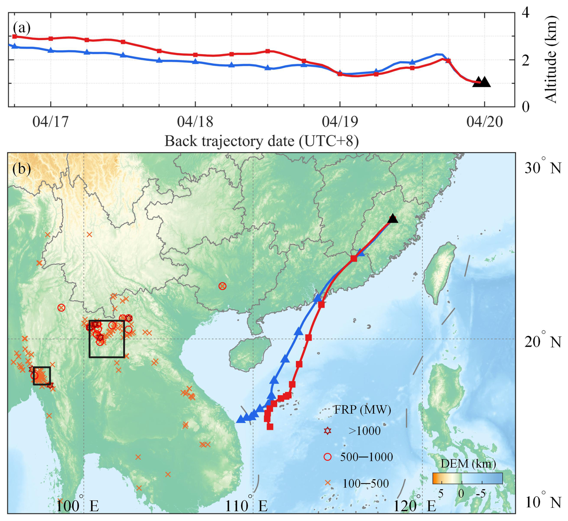
Figure B1 HYSPLIT backward trajectory analysis initialized at 1 km (the LIF lidar site marked by black triangle). (a) Vertical variation of air mass altitude for the study period. (b) Horizontal (longitude-latitude) trajectories overlaid on presumed vegetation fire locations; marker colors and shapes indicate FRP levels.

Appendix C: Fluorescence spectra of previous studies

Zhang et al. (2019)Pan et al. (2012)Muller et al. (2008)Klapper et al. (2002)Louzon et al. (2025)

Table C1 Previous in-situ studies showing fluorescence signatures similar to the BBA spectrum observed in Case 1.

Reichardt et al. (2025)Veselovskii et al. (2025a)

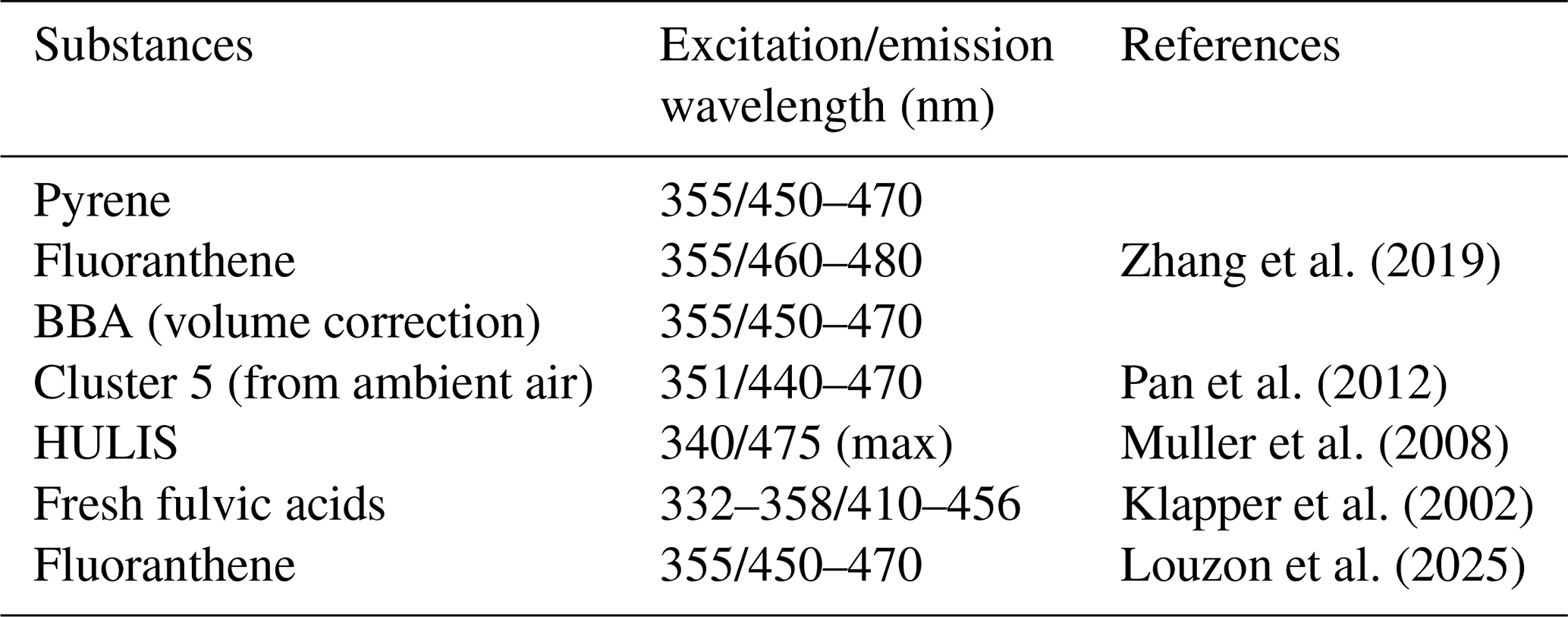
Table C2 Previously reported LIF lidar fluorescence peaks of BBA.