Improved method for temporally interpolating radiosonde profiles in the convective boundary layer

A significantly improved technique for temporally interpolating radiosonde (RS) profiles of potential temperature and water vapor mixing ratio in the planetary boundary layer during daytime is introduced. The key innovation of this technique is its operation on a height grid normalized with the planetary boundary layer height. This study utilized a three-month dataset of three-hourly soundings from the Atmospheric Radiation Measurement Facility's Southern Great Plains site. The technique was evaluated for convective boundary layer cases, with the necessary boundary layer height data obtained from a ground-based infrared spectrometer. A total of 79 comparisons were conducted between reference soundings and interpolated profiles that did and did not employ height normalization. The results demonstrated a substantial improvement in the representation of interpolated profiles using the new technique, characterized by enhanced correlation, improved amplitude representation, and reduced bias for potential temperature, as well as improved correlation and reduced bias for water vapor mixing ratio.

1 Introduction

Atmospheric science relies heavily on radiosonde (RS) soundings, which provide an accurate, high vertical resolution method of profiling the atmosphere. From the surface to altitudes of 20 to 30 km, RSs conduct measurements of temperature, pressure, humidity, and wind during their ascent with high frequency and under all weather conditions (Jensen et al., 2016; Wulfmeyer et al., 2015).

This dependency on RSs has drawbacks, as the sounding locations are relatively scarce (Wulfmeyer et al., 2015), the soundings are not vertical, and the launches occur routinely only two to four times per day at many operational sites, such as the ones operated by the Atmospheric Radiation Measurement (ARM) Facility (Jensen et al., 2016), which also incorporates the Southern Great Plains (SGP) site considered in this study.

However, many applications require a higher temporal resolution than 6 or 12 h. The study of turbulent transport processes (e.g., Wulfmeyer et al., 2016; Gibert et al., 2025), the feedbacks between land and atmosphere (e.g., Santanello et al., 2018; Wulfmeyer et al., 2020), as well as many other fields of atmospheric research, rely on high-resolution vertical profiles of temperature and humidity. A concrete example of this need, and initial motivation behind the presented study, is the investigation of the latent heat entrainment flux at the top of the convective boundary layer (CBL). This requires high-resolution data of humidity and vertical wind (Wulfmeyer et al., 2016), both available as lidar data products at the ARM SGP site (Newsom and Sivaraman, 2018; Newsom and Krishnamurthy, 2022). What is also required, but not available, is a temporally and vertically high-resolution profile of potential temperature that can capture, especially, the strong gradient at the top of the CBL at an arbitrary time. The noise levels of the ARM SGP Raman lidar are too high for this purpose (Osman et al., 2019), and the simple RS interpolation product (Fairless et al., 2021) by ARM, which linearly averages the nearest soundings on a fixed height grid, fails in recreating the actual structure of the CBL (demonstrated later). To address this need, this study proposes an improved interpolation technique.

The mentioned ARM Interpolated Sonde product is the benchmark for this proposed improved technique. However, the actual ARM product is not used explicitly in this work, but rather a “simulation” of it for yet-to-be-explained reasons.

The improvement proposed in this work is straightforward. Rather than interpolating between two soundings on a fixed height grid, the new technique employs a normalized height grid, which is obtained by dividing the standard height grid by the planetary boundary layer height (PBLH) (Rosenberger et al., 2024). Normalizing the boundary layer profile with the PBLH to investigate the lower atmosphere is generally not a novel approach; an early example of this technique can be found in Augstein et al. (1974). For the time being, the applicability of this new technique is limited to the case of a CBL. The CBL consists of the unstable surface layer, the mixed layer where turbulence brings potential temperature and humidity to a relatively constant value with height, and the interfacial layer that separates the free atmosphere (FA), characterized by gradients in temperature and moisture, which also signify the PBLH (Stull, 1988). The relative heights and corresponding temperature and humidity levels of these layers may change throughout the day, but the overall layering remains, which is exactly the fact that the new technique exploits. Therefore, knowledge of the PBLH enables scaling soundings to the same relative height levels and interpolating only physically related regimes. To be precise, this study utilizes soundings of the boundary layer that took place between the morning transition and the afternoon decay. Especially the included soundings at 23:30 UTC might therefore take place during an on-setting decoupling of the lower and upper parts of the boundary layer as the turbulence generation at the surface grows weaker. However, the corresponding profiles are very similar in their structure to clear CBL profiles with a well-mixed/residual layer and an inversion layer above.

It is conceivable that a physically meaningful interpolation is already possible when the external PBLH estimate is replaced by an interpolation of the two PBLHs of the input soundings, as this would avoid the production of non-physical artifacts by averaging different atmospheric regimes. However, it can be expected that this approach can be a compromise at best, as this does not consider the non-linearity of the temporal CBL development, as it can be seen, e.g., in the Raman lidar observed humidity cross-section in Fig. 1g.

The proposed interpolation technique should therefore apply to all atmospheric situations that exhibit a similar temporal behavior and vertical structure in the CBL with clearly identifiable layers. Another example is the nighttime boundary layer, consisting of a stable boundary layer and a residual layer, and with clear expectations for the profiles of temperature and humidity (Stull, 1988). Although being limited to specific atmospheric situations may seem like a drawback, the case of the investigated CBL plays a unique role in atmospheric science. Intensive research is conducted on the CBL as it is essential for understanding atmospheric processes and feedbacks (e.g., Wulfmeyer et al., 2016; Behrendt et al., 2020).

Applying this new interpolation technique requires a time-wise continuous and smooth PBLH estimate. Fortunately, and as briefly discussed later, there are different available techniques utilizing different types of instruments, increasing the possibility that even smaller measurement sites can produce such an estimate. The chosen PBLH product depends, of course, on the underlying instrumentation and subsequent processing, and will not be a perfect representation of the actual PBLH. To determine and correct for the relative difference in PBLH between the radiosondes and the “external” product, a bias correction is applied.

The primary scientific question of this study can be stated as follows: Does temporally interpolating RS profiles on a normalized height grid yield a more accurate representation of the vertical structure in the CBL compared to interpolating on a standard height grid?

This work focuses on the interpolation of potential temperature and water vapor mixing ratio (WVMR) profiles and begins with a concise overview of the data utilized and the underlying instrumentation in Sect. 2. The selection process for suitable soundings during CBL conditions and the interpolation technique are presented in Sect. 3. Thereafter, the results of this work are explained in Sect. 4, which includes an example case and a statistical analysis. Finally, the key findings are summarized in Sect. 5.

2 Observations

This study utilizes measurements and data products from the U.S. Department of Energy (DOE) ARM SGP site in Oklahoma, USA (Sisterson et al., 2016). The ARM facility aims to support atmospheric science by providing a broad spectrum of meteorological measurements collected in key climate regions. The SGP site covers a northern hemisphere, continental, mid-latitude area, providing a “continuous multivariable observationally based dataset” of the atmosphere (Sisterson et al., 2016). It is equipped with a wide range of surface-based and remote-sensing instruments, enabling synergies and intercomparisons of different data products. A detailed description of the site and the present atmospheric conditions is given by Krishnamurthy et al. (2021a).

This study uses data from 17 April to 21 July 2019, a period that is particularly well-suited for this research on RSs due to the frequent launches every 3 h as part of a special field campaign (Weckwerth et al., 2020). Additionally, PBLH time series data provided by the Tropospheric Remotely Observed Profiling via Optimal Estimation (TROPoe) algorithm, which retrieved temperature and humidity profiles from the Atmospheric Emitted Radiance Interferometer (AERI) at the site, as well as Raman lidar data, are used for a quantitative and qualitative comparison. During the period under review, sunrise occurred between 11:00 and 12:00 UTC, and sunset occurred between 01:00 and 02:00 UTC.

2.1 Radiosondes

Since the end of 2017, the Vaisala RS41 has been the standard RS model at the ARM SGP site. During its flight, the RS41 samples temperature, pressure, relative humidity, and wind at a rate of once per second, resulting in a height resolution of about 5 m for a nominal ascent rate of 5–5.5 m s⁻¹ (Holdridge, 2020). The corresponding data product also includes secondary quantities, such as dew point temperature and height above sea level (Keeler et al., 2001), which allows for the calculation of potential temperature and WVMR. For more details and a comparison with the previous RS model, see the work by Jensen et al. (2016).

Typically, launches take place every 6 h at 05:30, 11:30, 17:30, and 23:30 UTC. However, during the period under review, three-hourly launches were conducted, resulting in additional take-offs at 02:30, 08:30, 14:30, and 20:30 UTC (Weckwerth et al., 2020). This yields four to five soundings during daylight hours.

2.2 AERI and TROPoe

The required smooth time series of the PBLH is obtained through the TROPoe algorithm that retrieves thermodynamic profiles from the AERI. The AERI is an autonomous, passive, ground-based infrared spectrometer developed for the ARM facility and deployed to all of its primary sites, including the SGP site (Turner et al., 2016b). It measures downwelling radiance from the atmosphere with a radiometric accuracy better than 1 % of the ambient radiance, thanks to a precise calibration with two blackbodies (Knuteson et al., 2004).

Temperature and humidity profiles are retrieved from the AERI output via the TROPoe algorithm on a fixed vertical height grid with a resolution that exponentially decreases from 25 m near the surface to 800 m at a height of 3 km, while the temporal resolution of the used data product is 5 min. The TROPoe algorithm uses observations and a Gaussian a priori probability density function that describes the mean atmospheric state to iteratively estimate the current atmospheric conditions via a forward radiative transfer model. It can provide a complete error covariance matrix for the solution and has a mean bias of less than 0.2 K and 0.3 g kg⁻¹ for temperature and WVMR, respectively, under optimal conditions and atmospheric heights below 2 km (Turner and Löhnert, 2014). In addition to the primary variables, which include temperature and WVMR, the data product also includes other derived quantities, such as the required PBLH (Turner, 2010). The PBLH was determined using a parcel method (i.e., by lifting a parcel at the surface along a constant virtual potential temperature profile until it encountered a higher value above, following the approach by Nielsen-Gammon et al., 2008).

It should be noted that the use of AERI and TROPoe is not strictly necessary. The only essential requirement is the availability of a temporally smooth PBLH time series, which can originate from different active or passive remote sensing instruments (Duncan et al., 2022; Kotthaus et al., 2023), such as lidars, and can even include machine learning techniques (Krishnamurthy et al., 2021b). Any suitable data product could have been used for this purpose. However, the specific charm of AERI and TROPoe is their routine character, which makes them easily adoptable at other ARM sites. Regardless of what specific PBLH time series is used, it will contain a bias that will vary with the atmospheric conditions. This bias will impact the presented interpolation more or less, depending on its size. An attempt to reduce this impact is the employment of a bias correction, which is explained later.

At this point, it should be made clear that this study is about the demonstration of an improved interpolation technique utilizing additional PBLH information. In this specific demonstration, the value of the interpolated product is questionable, as it might be more straightforward to use the temporal high-resolution (compared to single soundings) thermodynamic profiles of TROPoe or the Raman lidar directly. However, the additional value of the proposed technique lies in the fact that it only requires the PBLH estimate as additional information. It is therefore conceivable that in a very limited setting, the only chance of retrieving profiles of potential temperature and humidity is the use of the presented technique, at least for a CBL. A fictional example could be a measurement site that only employs radiosondes and a Doppler lidar from which the necessary PBLH information is extracted (e.g., Sivaraman and Zhang, 2010 at the ARM SGP site).

To avoid any misunderstanding, deriving a continuous estimate of the PBLH is far from trivial and constitutes its own field of research. Numerous methods exist, often differing significantly in their results (for RSs, e.g., Seidel et al., 2010), and their performance depends on the atmospheric conditions and underlying instrumentation (e.g., Zhang et al., 2022; Kotthaus et al., 2023).

2.3 Raman lidar

It is desirable to compare the RS interpolation not only at a single point in time but throughout the entire daily cycle. For WVMR, this is achievable using the temporally and spatially high-resolution output of the SGP Raman lidar (Newsom and Sivaraman, 2018; Turner and Goldsmith, 1999; Turner et al., 2016a). Its functional principle is based on Raman scattering, which involves detecting and analyzing the energetic shift in the backscattered signal of the emitted laser pulses. These pulses have a wavelength of 355 nm and a frequency of 30 Hz. The raw data has a spatial resolution of 7.5 m and a temporal resolution of 10 s, although in this study, a data product with 10 min averages is used (Newsom et al., 2022).

Important to note is the fact that this data product is only used for a qualitative visual comparison and is not required for the presented interpolation itself.

3 Case selection and interpolation

From the three available months, those RS launches were selected, which took place within a CBL 6 or 9 h apart from one another. This allows for one or two intermediate soundings that can be compared to time-wise corresponding interpolations. Two different types of temporal interpolations were performed for these soundings. First, the interpolation without any height normalization (HN), which represents the current standard procedure used in the interpolated sonde product by ARM. And second, the newly proposed interpolation technique that utilizes a smooth PBLH estimate to normalize the height coordinate.

3.1 Case selection

The presented technique aims to improve the temporal RS interpolation for cases of a CBL. The temperature and humidity profiles exhibit a unique structure with clear layers, which provides the potential for an interpolation, as they can remain structurally similar through appropriate compression or stretching.

The corresponding soundings from April to July 2019 were selected by manually inspecting the potential temperature profiles for characteristics indicative of a CBL, i.e., relatively constant values in the mixed layer and a pronounced gradient on top, signifying the interfacial layer. As a result, this study focuses on the daytime period, with launches available from 14:30 to 23:30 UTC. The 11:30 UTC launch, which coincides with sunrise, does not exhibit a clear CBL structure and is therefore excluded.

This selection process resulted in 79 available comparisons between the reference and interpolated soundings.

3.2 Interpolation without a height normalization

The “current” or “non-HN” temporal interpolation between two RSs, as routinely performed by the ARM facility (Fairless et al., 2021), is straightforward. To interpolate to a time of interest, the two closest soundings in time are vertically interpolated to a common fixed height grid with a resolution of Δz=20 m in the lowest 3.5 km. Then, for each height level, a linear interpolation in time is performed for the atmospheric state variables (Fairless et al., 2021).

However, ARM's routine data product is not used in this study, as it incorporates all three-hourly separated soundings, leaving no intermediate soundings for comparison. In other words, the ARM facility interpolates soundings that are 3 h apart from each other. Still, this study needs a product based on the interpolation of soundings that are 6 h apart from one another to use the additional soundings for the presented quantitative comparisons. Therefore, the non-HN interpolation is implemented manually on a fixed height grid with a spatial resolution similar to ARM's.

3.3 Interpolation with a height normalization

The key distinction of the “new” interpolation method lies in its operation on a normalized height grid $\widehat{z}$, which takes into account the daily development of the CBL. Rosenberger et al. (2024) demonstrated the potential benefits of this method by showing that autocovariance analysis of high temporal resolution lidar data of vastly changing PBLHs z_i leads to a better agreement of the higher moments close to z_i with reality, if it is executed on a normalized height grid. This normalized height grid is the standard height grid z divided by an appropriate temporal average of the PBLH z_i, resulting in the transformation $\widehat{z}=z{\stackrel{\mathrm{‾}}{z_i}}^{-\mathrm{1}}$. Consequently, a temporally smooth estimate of the PBLH $\stackrel{\mathrm{‾}}{z_i}$ is required.

Thus, the normalization ensures that only equivalent atmospheric layers are interpolated, thereby preventing nonphysical gradients. For instance, the center of a mixed layer is interpolated by averaging the centers of the mixed layers at the times used for the interpolation. This principle applies to all height levels. Crucially, there is no nonphysical interpolation between an earlier interfacial layer and a later mixed layer at the same height level.

For the interpolation procedure, potential temperature and WVMR are calculated for the input soundings. The corresponding PBLHs are identified by automatically searching for the height between 100 and 2500 m where the potential temperature gradient peaks. This simple method can lead to false identifications, but the improvement of this is left for future work. Here, the main interest lies in the statistical investigation of many interpolated soundings in comparison to their reference profile, and not in the quality of a single interpolation.

As the temporal interpolation will be performed on a normalized height grid, the identified PBLHs are used to normalize the corresponding profiles. The PBLH at the time of interest is extracted from the TROPoe time series data, which is smoothed using a 30 min moving average. When compared to high-resolution Raman lidar data (not shown), which is expected to offer the best estimate of the PBLH, the retrieved estimate is not always accurate. To address this, a bias correction is applied, which linearly interpolates the bias between the PBLH estimate from TROPoe and the gradient peak of the RSs at the two launch times to the time of interest. The normalized “target” height grid at this time can then be defined by dividing a fixed height grid with a Δz=20 m resolution by the corresponding smoothed and bias-corrected PBLH $\stackrel{\mathrm{‾}}{z_i}$.

Next, the two normalized RS profiles are spatially linearly interpolated to the normalized height grid of the time of interest. Now, on the same normalized height level, the temporal interpolation is performed. The subsequent quantitative analysis operates on the normalized height grid, as only this allows for meaningful height-related comparisons between different pairs of interpolated and reference profiles.

4 Results

First, the presented interpolation technique is qualitatively evaluated by comparing time-height cross-sections of WVMR for a day with a well-developed CBL. Both interpolation techniques, as well as the “true” state of the atmosphere represented by the temporally and spatially high-resolution measurements of a Raman lidar, are compared. This qualitative assessment is followed by a quantitative analysis, in which for each interpolation technique, the same 79 interpolated profiles are compared to the corresponding reference profiles in terms of their correlation, their ratio of standard deviations, and their bias. Each comparison between two profiles is called a “case” from now on, meaning that there are 79 cases of either interpolation technique that can be analyzed in terms of the mentioned metrics.

4.1 Example case

Figure 1 presents time-height cross-sections of WVMR m for 24 June 2019, between 14:29 and 23:33 UTC from the two interpolations (without an HN in (a), (c), and (e); with an HN in (b), (d), and (f)) and the Raman lidar (same cross-section in (g) and (h)). The interpolations were performed between soundings (dashed lines) that launched 6 (first two rows) or 9 (third row) hours apart from each other. Compared is a cross-section from the continuously measuring Raman lidar with 10 min average values. Consequently, the same temporal resolution was applied for the interpolation.

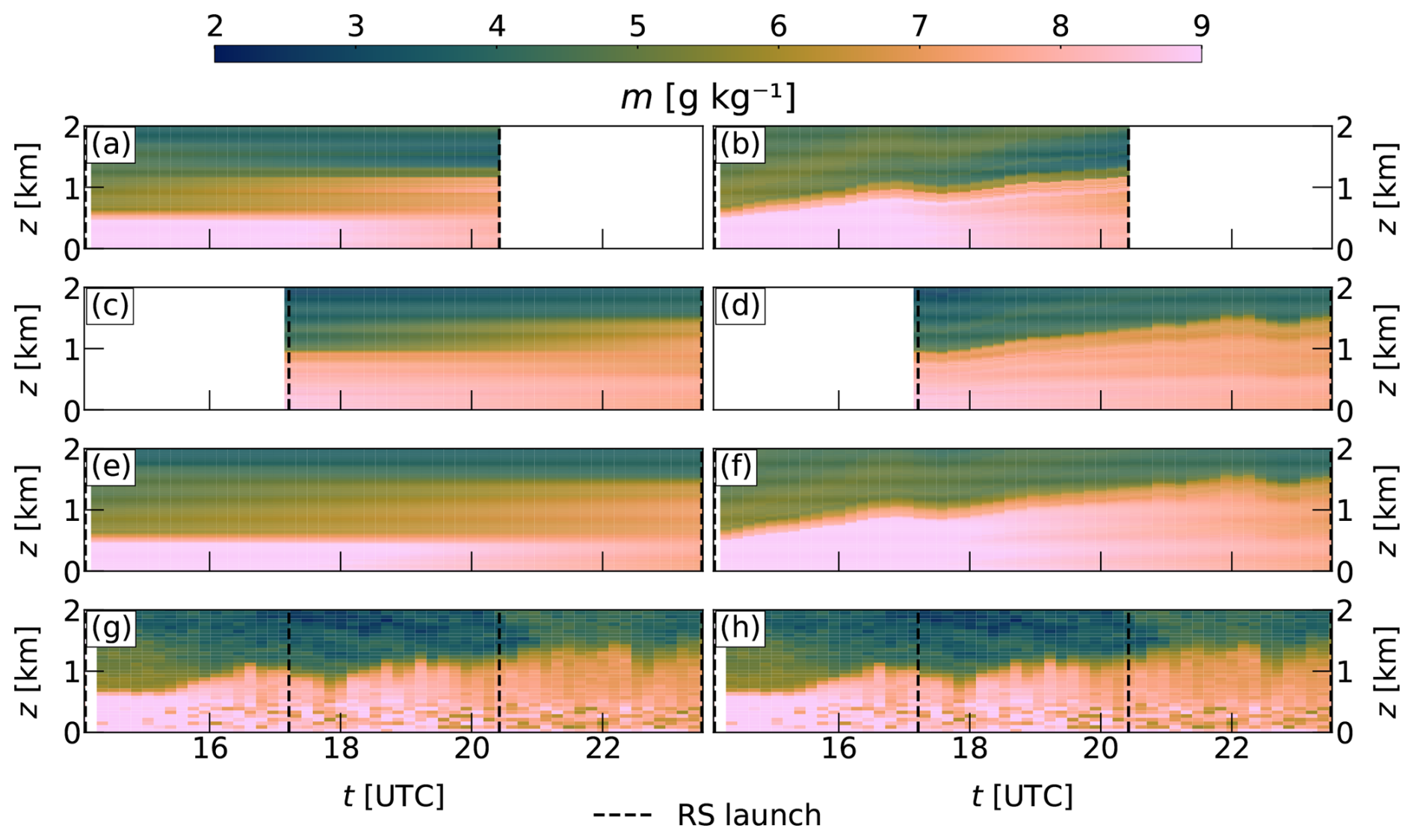
Figure 1 Time-height cross-sections of WVMR m for 24 June 2019, between 14:29 and 23:33 UTC are shown for the RS interpolation on a standard height grid (a, c, e), on a normalized height grid (b, d, f), and from a Raman lidar (g, h). The RS interpolations were performed between the following soundings (dashed lines): (a, b) between 14:30 and 20:34, (c, d) between 17:29 and 23:32, and (e, f) between 14:30 and 23:32 UTC. The utilized color map comes from the Python package of Crameri et al. (2020).

It is immediately evident that the new interpolation technique provides a more accurate representation of atmospheric conditions in the CBL, as confirmed by the Raman lidar. While the Raman lidar is not perfect, as the noise in the lower parts of the mixed layer demonstrates, it continuously observes the overall structure (layering) of the CBL. This structure is much better represented by the interpolation that utilizes an HN, which holds for all three covered time intervals, even the ones that span 9 h. In contrast, the non-HN interpolation method fails to approximate the observed CBL structure even roughly, a deficiency that becomes particularly evident at the 9 h intervals between soundings.

In this specific instance, the proposed interpolation technique demonstrates clear superiority over the method routinely used by the ARM facility. Consequently, the question arises whether this is an isolated favorable example or a statistically significant improvement.

4.2 Statistics

The quantitative analysis presented here leverages the additional RS launches during the selected months to address this question. For this period, interpolations between launches that are 6 or more hours apart are performed, which is consistent with the standard procedure at the SGP site (Holdridge, 2020). However, these launches are now interpolated to the time of the intermediate soundings, enabling a quantitative comparison. For example, the soundings at 17:30 and 23:30 UTC are interpolated so that the time of the additional sounding at 20:30 UTC is covered. To be clear, the interpolated sondes of both methods are compared to soundings that are not used in the corresponding interpolations.

By focusing exclusively on CBL situations and normalizing with the PBLH, the new interpolation technique is specifically designed to improve the structural representation within the daytime planetary boundary layer (PBL). As a result, this analysis focuses on height levels from the ground up to 1.2 times the PBLH, ensuring coverage of the interfacial layer. Both interpolated profiles, as well as the reference profile, are spatially interpolated onto a fixed normalized height grid with a spacing of $\mathrm{\Delta }\widehat{z}=\mathrm{0.05}$, resulting in 25 height levels that can be compared for each case. This requires transforming the interpolation without an HN and the reference profile to this normalized height grid, which is achieved using a manually validated PBLH estimate to guarantee a meaningful comparison between the different profiles.

4.2.1 Correlation and amplitude

To assess the performance of the two interpolation methods, the structure of the reference profile is first examined to determine how well it is approximated by the interpolations within the specified height interval. For this purpose, Pearson's correlation coefficient r and the ratio of the standard deviations of the interpolated and the reference profile ${\mathit{\sigma }}_{\text{interp}}/{\mathit{\sigma }}_{\text{ref}}$ are calculated for every selected comparison, respectively. r indicates how well the compared profiles vary together (Stull, 2017), or in other words, how well the interpolation can recreate the structure (here primarily the layering) of the actual profile. The ratio ${\mathit{\sigma }}_{\text{interp}}/{\mathit{\sigma }}_{\text{ref}}$ describes how well the amplitude of the structural variations is represented (Taylor, 2001). In the context of a CBL with a mixed layer that is signified by nearly constant values of potential temperature and WVMR as well as a sharp gradient over the interfacial layer for those quantities, a well-reproduced structure would imply that ${\mathit{\sigma }}_{\text{interp}}/{\mathit{\sigma }}_{\text{ref}}$ correctly captures the amplitude of the gradient if this ratio is equal to unity. However, to ensure that over- and underestimations of the amplitude of the same absolute factor 2^(−)x with $x\in {\mathbb{R}}_{\mathrm{0}}^{+}$ are weighted in the same way, the binary logarithm of this ratio ${\log }_{\mathrm{2}}({\mathit{\sigma }}_{\text{interp}}/{\mathit{\sigma }}_{\text{ref}})$ is considered because ${\mathit{\sigma }}_{\text{interp}}={\mathrm{2}}^{(-)x}{\mathit{\sigma }}_{\text{ref}}\iff (-)x={\log }_{\mathrm{2}}({\mathit{\sigma }}_{\text{interp}}/{\mathit{\sigma }}_{\text{ref}})$. Hereafter, this logarithmic ratio is also referred to as “the amplitude”.

It is essential to note that both r and ${\mathit{\sigma }}_{\text{interp}}/{\mathit{\sigma }}_{\text{ref}}$ represent the entire selected height profile, extending up to 1.2 times the PBLH. Figure 2 illustrates the scatter plot of these metrics for the 79 cases, distinguishing between interpolations with (red) and without (blue) an HN, for (a) potential temperature θ and (b) WVMR m. The figure also differentiates between cases interpolated over 6 h intervals (dots) or 9 h intervals (crosses). The semi-transparent planes visualize how close most of the data points for the HN and non-HN interpolation are to the ideal values of r=1 and ${\log }_{\mathrm{2}}({\mathit{\sigma }}_{\text{interp}}/{\mathit{\sigma }}_{\text{ref}})=\mathrm{0}$ respectively by being spanned by those 85 % that are closest.

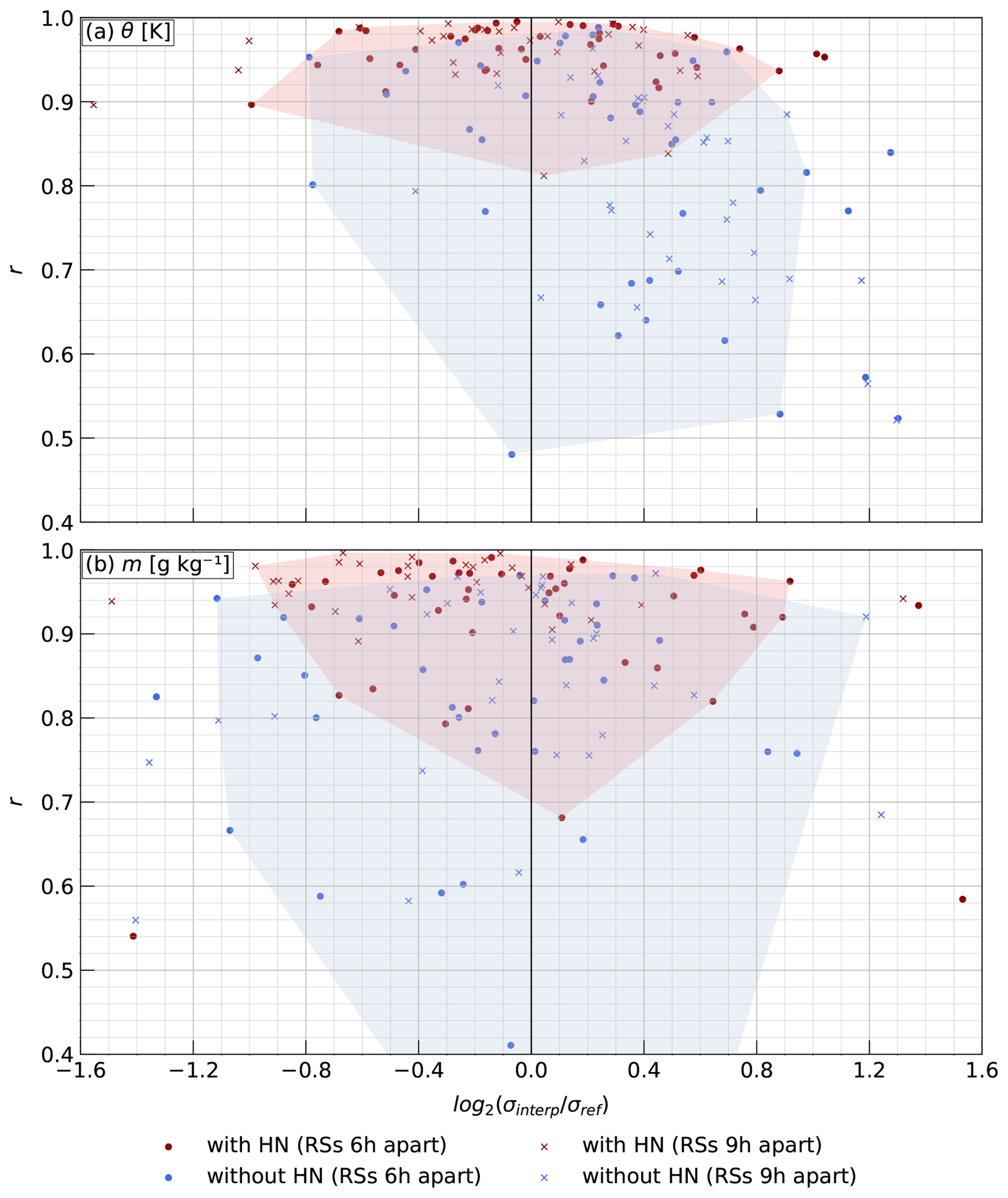
Figure 2 Distributions of the 79 profiles are shown for the interpolation with (red) and without (blue) an HN. Each interpolation is characterized by its correlation (r) to the reference profile and the binary logarithm of the normalized standard deviation (${\log }_{\mathrm{2}}({\mathit{\sigma }}_{\text{interp}}/{\mathit{\sigma }}_{\text{ref}})$) of the whole profile for (a) potential temperature θ and (b) WVMR m. Points represent interpolations where the used RSs were launched 6 h apart, while crosses mark interpolations where this time difference was 9 h. For better visualization, twelve data points (seven with and five without an HN) are not shown in (a), as well as 16 data points (six with and ten without an HN) in (b). This results in 72 and 74 data points shown in (a) for HN and non-HN interpolations, respectively. In (b), 73 and 69 data points are shown, respectively. The shown planes are spanned by those 85 % of data points that are closest to the ideal values of r=1 and ${\log }_{\mathrm{2}}({\mathit{\sigma }}_{\text{interp}}/{\mathit{\sigma }}_{\text{ref}})=\mathrm{0}$.

The scatter plot of cases reveals that the interpolation interval (6 or 9 h) does not appear to have a significant impact, so that any potential differences related to this are not investigated further. It is evident that the interpolation with an HN leads on average to higher correlations, as most cases cluster closely around r = 1, whereas the interpolation without an HN exhibits a larger spread to lower correlation coefficients. This is observed for both variables, but is particularly pronounced for potential temperature. Additionally, the interpolation without an HN appears to produce more cases with larger deviations in amplitude. This is visualized especially well by the shown planes. The plane that is spanned by those 85 % of data that is closest to the ideal values is obviously smaller for the HN interpolation than for the non-HN one, representing a smaller spread to less ideal values.

Notably, there is a cloud of cases for potential temperature interpolated without an HN that have lower correlation coefficients between 0.6 and 0.9 and a systematic overestimation of the actual amplitude. These cases can be readily explained and highlight the limitations of the current interpolation method. Upon closer examination of individual interpolations (not shown), it turns out that these low correlations are often associated with the introduction of nonphysical atmospheric layers as artifacts of insufficient interpolation, which are then incorporated into the analyzed height levels. For example, averaging an early-day potential temperature sounding with a lower PBLH together with a later-day sounding that has a higher PBLH (using the non-HN technique) will produce an apparent extra “layer” at heights where the warmer free atmosphere from the first sounding is averaged with the cooler mixed layer from the second. However, additional layers with a change in potential temperature increase the profile's variability compared to a single mixed layer capped by a gradient.

The results presented in Fig. 2 are summarized in Table 1, which provides the median, mean, and standard deviation of the correlation and the amplitude for the profile comparisons of the two variables (potential temperature and WVMR) and interpolation techniques (with and without an HN). To determine whether the interpolation with an HN yields significant improvements over the interpolation without an HN, a two-sided paired permutation test was conducted. This statistical test was chosen because it is well-suited for comparing two samples consisting of matched pairs drawn from unknown distributions. This test function is available in the widely used SciPy Python package (Haberland, 2023). The test statistic is based on the difference between the sample means, medians, or standard deviations. A total of 10 000 permutations were performed. The null hypothesis states that the data are randomly assigned to samples. If the null hypothesis is accepted, it implies that the interpolation techniques do not produce significantly different results. It is rejected when the probability of obtaining the observed result under the null hypothesis is less than 5 %. More information on SciPy can be found in Virtanen et al. (2020). A comprehensive introduction to permutation tests can be found in LaFleur and Greevy (2009). Values that show significant improvement over the other interpolation technique are bolded.

Table 1 Comparison of the median (Median), mean (Mean), and standard deviation (SD) of Pearson's correlation coefficient (r) and the binary logarithm of the normalized standard deviation (${\log }_{\mathrm{2}}({\mathit{\sigma }}_{\text{interp}}/{\mathit{\sigma }}_{\text{ref}})$) between the interpolation on a normalized height grid and a standard height grid (with and without an HN respectively) are shown for potential temperature θ and WVMR m between 0.0 and 1.2 times the PBLH. This statistic is based on the 79 cases selected. Bolded values indicate a permutation-tested significant improvement of this metric for the corresponding interpolation technique over the other one.

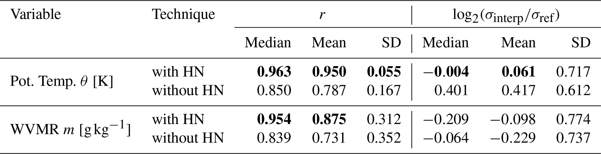
As already illustrated in Fig. 2, the improvement of the interpolation with an HN is particularly pronounced for potential temperature. Its median and mean values for the correlation and the profile amplitude are significantly improved. The median correlation increases from 0.850 to 0.963, and the median amplitude decreases from 0.401 to −0.004, bringing both values much closer to the ideal values of r=1 and ${\log }_{\mathrm{2}}({\mathit{\sigma }}_{\text{interp}}/{\mathit{\sigma }}_{\text{ref}})=\mathrm{0}$. Furthermore, the standard deviation for the correlation is also improved, with a significantly smaller value of 0.055 compared to 0.167.

This picture is less clear for WVMR. Although the correlation is significantly improved, with a median of 0.954 compared to 0.839, the standard deviations are much higher and of comparable magnitude, at 0.312 and 0.352. The amplitude of the interpolated WVMR profiles is not improved (but also not worsened), as the median value of the interpolation without an HN is closer to the ideal value of 0, while for the mean, it is the value of the interpolation with an HN that is closer. The standard deviations are comparable, at around 0.75.

Overall, the new interpolation represents a clear improvement in approximating the structure and amplitude of potential temperature profiles in the convective PBL. The structure of WVMR profiles is also better represented with the new technique, although the picture is less clear for its amplitude. It is worth noting that WVMR profiles are generally more challenging to interpolate accurately, as moisture is significantly affected by different sources at the surface, advection, and cloud formation, exhibiting more visible variations in individual profiles (Stull, 1988). Please note that the new interpolation technique is proposed to improve profiles within the convective PBL. Table 2 therefore shows the same statistics for the correlation and amplitude representation for the height interval between 0.0 and 1.0 PBLH.

Table 2 Analog to Table 1 but for the height interval between 0.0 and 1.0 PBLH.

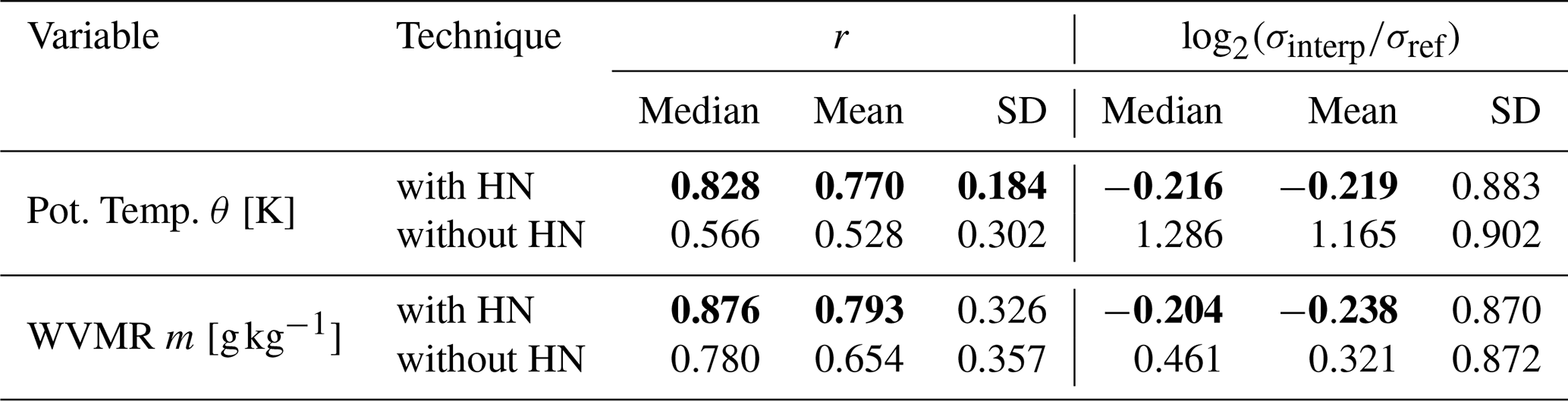
Although the absolute values for correlation and amplitude seem degraded, as they lie for both techniques farther away from the ideal values of r=1 and ${\log }_{\mathrm{2}}({\mathit{\sigma }}_{\text{interp}}/{\mathit{\sigma }}_{\text{ref}})=\mathrm{0}$, the significant improvements of the new method compared to the current one stay the same. Now, even the median and mean values of the amplitude representation for WVMR are significantly improved from 0.461 to −0.204 in the case of the median. The reduced absolute values are no surprise, as this adjusted height interval does not encompass the (full) gradient in potential temperature or WVMR, and with that has much less structure that can be captured and compared.

4.2.2 Bias

After determining how well the two interpolation techniques perform in terms of their ability to recreate the reference profile's structure and amplitude, the bias must be quantified. This is necessary because the previously discussed metrics may indicate a more accurate representation of the shape of the reference profile. However, they are blind to the possibility that the interpolated profile may result in a completely different temperature or humidity value.

The following analysis of the bias is conducted in a height-resolved manner, meaning that for each of the 25 available height levels, the bias is calculated for all 79 cases. Figure 3 presents the height profiles of the mean bias (first column) and its standard deviation (second column) for the interpolation with (red) and without (blue) an HN for potential temperature θ (first row) and WVMR m (second row).

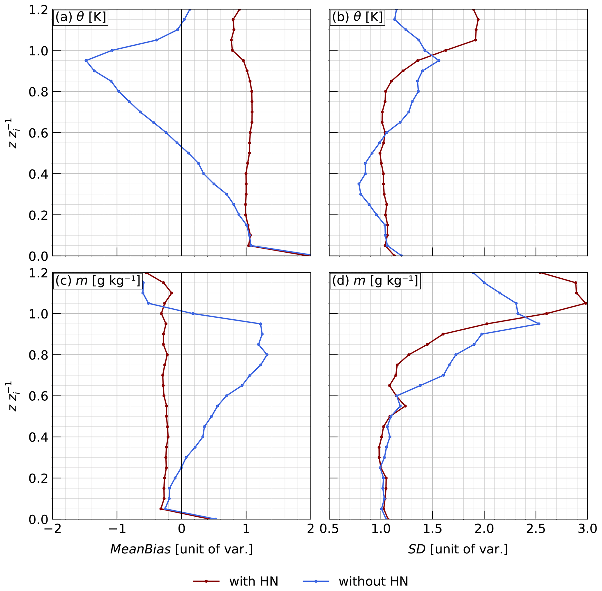
Figure 3 Profiles of (a, c) the mean bias (MeanBias), calculated as the reference value minus the interpolated value, and (b, d) its standard deviation (SD) are shown for different normalized height levels between 0.0 and 1.2 times the PBLH with z_i = PBLH for (a, b) potential temperature θ and (c, d) WVMR m with (red) or without (blue) an HN. Bias and standard deviation have the same units as the corresponding variable.

Upon examining the results, it is readily apparent that neither interpolation technique is perfect, as both exhibit a non-zero bias. However, it is also clear that the interpolation with an HN displays a relatively constant bias and standard deviation profile throughout the investigated height interval, facilitating a more meaningful correction if the corresponding bias can be estimated. This is a further argument for the good structural representation of the reference profile. The interpolation without an HN does not achieve this.

Returning to the actual meaning of the bias, it is visible that the new interpolation exhibits a mean cold bias of approximately 1 K and a mean wet bias of approximately 0.3 g kg⁻¹, with corresponding standard deviations of about 1 K and 1 g kg⁻¹ in the mixed layer. This bias arises from underestimating potential temperature and overestimating WVMR. The presence of a bias is not surprising, given that the temporal interpolation is still linear and thus unable to capture mesoscale, or generally non-linear, changes in overall temperature and humidity levels that occur over time due to the sun's varying energy input. A concrete example is the sounding at 14:30 UTC in the morning with generally cooler conditions than the reference conditions later in the day. Potential temperature profiles that were interpolated using this sounding have an especially pronounced cold bias (not shown).

The mean bias of the interpolation without an HN changes roughly linearly with height, reaching a negative (potential temperature) or positive (WVMR) value at the PBLH of comparable or even greater magnitude than the new interpolation. In other words, the two bias profiles diverge increasingly with height. The standard deviation also varies more and takes on larger values in the upper part of the mixed layer, between 0.6 and 0.95 PBLH. This limits a general scientific application of the current interpolation technique.

Focusing on potential temperature, this behavior can be understood by considering the mentioned cold bias and the fact that the interpolation technique does not use an HN. This causes nonphysical artifact layers in the resulting profile. For the height levels close to the surface, it is evident that the choice of the technique has a minimal impact, as corresponding physical regimes are averaged. For instance, parts of the mixed layer from the earlier and later soundings are averaged, resulting in a mixed layer that is likely to be present at the time of interest. The new interpolation technique can be superior, as it consistently averages corresponding fractions of the boundary layer, but this effect is small for a mixed layer with a nearly constant potential temperature profile.

However, as the height increases to around 0.2 PBLH, there will be the first cases for which the interpolation without an HN averages different physical regimes, as the earlier sounding has a shallower PBLH (Stull, 1988). In this study, this comes down to the soundings at 14:30 UTC, which introduce a pronounced cold bias into the resulting profile. At these height levels, the interpolation without an HN averages the FA of the earlier sounding with the mixed layer of the latter. Since the FA is warmer than the underlying mixed layer (Stull, 1988), the potential temperature of the introduced artifact layer can be closer to the actual temperature or exhibit a warm bias resulting in a statistically smaller mean bias and standard deviation for this height compared to the interpolation that utilizes an HN.

This explanation is supported by the fact that the divergence of the bias profiles begins at higher height levels, and the standard deviation remains roughly constant when cases using the sounding at 14:30 UTC are excluded (not shown). Going up in height, more and more cases of the non-HN interpolation introduce an artificial layer, shifting the mean bias towards larger and larger warm biases and increasing its standard deviation. At a height level around the PBLH, approximately 0.95 times the PBLH, the absolute mean bias decreases again, as the reference profile has reached the FA.

From about 0.8 times the PBLH, the standard deviation of the bias increases drastically with height for the HN interpolation. The reason for this is the insufficient representation of how the gradients that characterize the interfacial layer are shaped. The HN interpolation can interpolate the information that there is a gradient (which defines the PBLH), but there is no information about the shape of this gradient at the time of interest. As this shape can vary greatly, e.g., the magnitude of the curvature, the onset of the gradient, or its steepness, the chance is high that the shapes of the interpolated and reference gradient are not very comparable, which translates into a broader spread in the biases at these heights. It must be stressed here that, although this might be one of the weaker aspects of the new technique, already the fact that the PBLH is incorporated allows for this much more meaningful interpolation.

5 Conclusions

This work introduced a new and simple technique for temporally interpolating RSs in the atmospheric boundary layer, specifically in the CBL. The new method operates on a normalized height grid, unlike the standard height grid commonly used by institutions such as the ARM facility. Normalization is achieved using the PBLH, which enables the technique to average only physically related height levels during interpolation, thereby preventing the formation of nonphysical artifact layers.

The required PBLH estimates were derived from the processing of radiance interferometer data, although they could have been obtained from any source providing a temporally continuous PBLH estimate. A bias correction was applied to ensure that these estimates were consistent with the PBLH values derived from the radiosondes, which was necessary to achieve the improvements presented in this study.

The improvements of the new technique were quantified by comparing interpolated profiles of potential temperature and WVMR with actual soundings as well as with the routine interpolation method that does not employ a height normalization. The comparison examined the correlation, amplitude representation, and bias between the two interpolation techniques and the reference sounding.

For the potential temperature, all metrics indicate a significant improvement of the new technique over the non-HN one. The median correlation of 0.963 and the amplitude of −0.004 are closer to the ideal values of 1 and 0, respectively, than the interpolation without height normalization. The bias remains approximately constant at 1 K throughout the boundary layer height interval, whereas the current interpolation method's bias varies with height, suggesting a poor structural representation that manifests itself as biases that appear statistically improved at certain height levels. Similar significant improvements in correlation and bias are observed for WVMR, although the representation of amplitude is only improved when changing the top of the investigated height interval to 1.0 times the PBLH.

Because the HN interpolation additionally requires the PBLH and is presently applicable only to CBL conditions as well as the boundary layer region, it is important to clarify its intended purpose. The routine, non-HN interpolation delivers thermodynamic profiles for the entire troposphere under all atmospheric regimes and therefore remains the best choice when continuous temporal and spatial coverage is required. By contrast, when the goal is to obtain the most accurate representation of thermodynamic conditions within the boundary layer during a CBL situation, the HN interpolation can provide a substantial improvement. It is not meant to replace the standard interpolation product, but rather to complement it for the specific use cases of boundary layer analysis.

In the future, it is important to investigate the performance of the new technique in various atmospheric situations beyond the CBL. Notably, time-wise structurally constant settings, such as a nighttime boundary layer, appear to be particularly promising. Additionally, a future focus should lie on exploring possibilities to simultaneously get the best results for the CBL, as well as the FA.

In conclusion, the initial question and objective of whether temporally interpolating on a normalized height grid yields an improved representation of reality in the lower atmosphere compared to interpolating on a standard height grid can be answered affirmatively. The presented method is recommended over the currently used one when feasible, as it benefits research and more sophisticated data products.