Synergistic Fusion of Aerosol Optical Depth over India from multi-sensor satellite retrievals with ground-based measurements

Synergistic fusion of aerosol parameters from multi-sensor measurements is crucial for integrating diverse data sources and generating consistent representations of aerosol distribution for accurate climate impact assessment. In this study, satellite observations from MODIS (Moderate Resolution Imaging Spectroradiometer) and MISR (Multi-angle Imaging SpectroRadiometer) are combined with ground-based measurements from the ARFINET and AERONET to generate fused Aerosol Optical Depth (AOD) over India. The primary focus of this study is to develop a fusion framework, involving the evaluation and comparison of two approaches: geostatistical Universal Kriging (UK) and a novel hybrid Residual Kriging – Machine Learning (RK-ML). Both methods share the same geostatistical foundation (variogram-based spatial-modeling) but differ in how the mean structure of AOD is estimated. In UK, satellite-retrieved AOD serves as deterministic trend for spatial prediction and is effective when ground-based observations are well distributed, whereas RK-ML considers ML (SVR) predicted AOD as prior and applies Ordinary Kriging to interpolate residuals from real-time ground observations, maintaining a near-zero residual mean away from observations which reduces distortion under sparse and uneven data conditions. Our results highlight seasonal fused AOD maps resembling very close to ground-based AOD over India. Leave-One-Out Cross-Validation (LOOCV) is adopted as an evaluation strategy for assessing performance, showing that fused AOD from both UK and RK-ML approaches captures up to 100 % of ground observations within the 95 % confidence interval (± 2σ), indicating effectiveness in capturing regional aerosol variability. RK-ML demonstrates more stable spatial patterns and improved LOOCV performance compared to UK, particularly in regions with limited ground-based coverage.

1 Introduction

Atmospheric aerosols play a significant role in introducing uncertainties into climate change projections. Although various factors such as microphysical parameters and the chemical composition of aerosols are important, aerosol optical depth (AOD), quantified by the total amount of columnar aerosol loading in the atmosphere, is the most critical parameter for understanding their climate forcing effects. With advances in technology and retrieval-algorithms, the number of satellites and ground-based observations of AOD is increasing. Although satellites are known to capture spatial heterogeneity of AOD, there could be bias or uncertainty (Huang et al., 2021) compared to ground-based measurements. Even if different satellites observe the same aerosol load over the same region nearly at the same time, the retrieved AOD differs due to the differences in algorithms, calibration, and resolution of the sensors (Kinne, 2009; Schutgens et al., 2020). The geographical complexity also challenges satellites to accurately retrieve AOD over highly heterogeneous land surfaces. On the other hand, data from ground-based sensors, though sparsely distributed, are more reliable than satellite measurements due to improved accuracy of measurement and retrieval procedure (Holben et al., 1998; Moorthy et al., 2007). Thus, the discrepancy between various satellite measurements and between satellite- and ground-based measurements of AOD is a serious concern in accurately characterizing aerosol loading over different parts of the globe (Wong et al., 2013; Sogacheva et al., 2020). In this context, there is a considerable effort in improving aerosol retrieval accuracy using approaches such as synergy processing of sun-photometer and lidar observations (Jin et al., 2025), synergistic retrieval from multi-mission space-borne measurements (Litvinov et al., 2025), gap-filling based on improved tensor-flow-based method (Bai et al., 2024), and the application of physics-informed deep-learning framework to multi-angle polarimetric measurements (Tao et al., 2023). Several studies have reported that if the correlations between the AOD from multiple ground-based and space-based sensors are sufficiently strong (Liu et al., 2004; Jiang et al., 2007; Prasad and Singh, 2007), then these observations can be used together for optimal characterization of aerosol features over a broader region. Thus, there is a growing demand for fused products to address limitations and achieve an optimal outcome, thereby strengthening reliability of aerosol database (Kahn et al., 2023).

Several approaches have previously been developed for multi-sensor data fusion involving satellite-to-satellite and satellite-to-ground observations. One notable method is the use of point spread function (PSF) modeling for single scanning footprints (Gupta et al., 2008). While PSF-based techniques are widely applied in image fusion, they face challenges in achieving accurate spatiotemporal colocation across different satellite platforms and don't show applicability regarding ground based AOD fusion rather solely on satellite footprint as a weighting factor for the merging of AOD from different sensors, such as MODIS (Moderate Resolution Imaging Spectroradiometer), MISR (Multi-angle Imaging SpectroRadiometer) and Clouds and the Earth's Radiant Energy System (CERES). Statistical approaches such as Maximum Likelihood Estimation (Kim et al., 2024; Nirala, 2008) and Bayesian Maximum Entropy (Tang et al., 2016) have been applied to integrate satellite and ground-based observations. These methods explicitly account for uncertainty; but, their practical implementation is often limited by high computational demands, as they require large datasets for effective sampling and detailed pixel-level uncertainty characterization to produce reliable fused products. Similarly, approaches such as the Ensemble Kalman Filter (Li et al., 2020) improve uncertainty quantification and have been applied at the global scale; however, their application is constrained by substantial computational cost and data requirements. These limitations pose challenges for near-real-time applications and for achieving high regional accuracy, particularly in regions with limited ground-based observational support. Least-squares-based approaches, including adaptive weighted estimation (Guo et al., 2013) and semi-empirical optical algorithms (Xu et al., 2012), offer computational efficiency; however, their validation and broader applicability remain uncertain. More recently, machine learning techniques, particularly deep neural networks (DNN) (Kim et al., 2024), have demonstrated comparable performance, but their dependence on large training datasets and challenges in generalization limit their practical deployment.

In this study, we have adapted the Kriging technique to produce optimal fused AOD products over India. Among the various data fusion techniques, Kriging has gained significant attention for its applicability under geostatistical framework and has long been recognized as a robust and effective geostatistical technique for spatial estimation (Zimmerman et al., 1999; Shi et al., 2007; Singh and Verma, 2019; Stein and Corsten, 1991; Zhao et al., 2017). Notably, though geostatistical approaches provide a promising framework for data fusion, they are constrained by high computational demands, particularly when incorporating both spatio-temporal autocorrelation and covariance matrix inversion. Hence, reduced-rank methods such as Spatial statistical data fusion (SSDF) (Puttaswamy et al., 2014; Nguyen et al., 2012) alleviate computational burden but may introduce overfitting due to the large number of parameters. In this context, Universal Kriging (UK) offers more stable AOD estimates near domain boundaries owing to its simpler and more robust formulation (Puttaswamy et al., 2014). Consequently, UK has been widely adopted for multi-sensor fusion integrating satellite and ground-based observations (Chatterjee et al., 2010; Puttaswamy et al., 2014; Lilla and Castrignanò, 2019), although it does not explicitly account for sensor-specific uncertainties. It has been extensively applied and validated across diverse domains within atmospheric research. It has also been utilized for spatial mapping of nutrients over oceans (Zhou et al., 2014) and as well as in mining, hydrology, electro-magnetic field mapping, and remote sensing image processing (Rossi et al., 1994). The Kriging outcomes are also found to be comparable with those from DNN (Chen et al., 2020; Kadow et al., 2020).

Previous research over the Indian region has estimated fused AOD from ground and satellite based observations using Cressman method, which employs inverse distance weighting (IDW), a widely used Geostatistical approach (Pathak et al., 2019). In this study, AOD measurements carried out from more than 40 ground-based observatories of the Aerosol Radiative Forcing over India Network (ARFINET; Fig. S1 in the Supplement; Babu et al., 2013; Gogoi et al., 2009), which constitutes the national network of aerosol observatories across India and the largest such network in South Asia, are primarily used to integrate with the satellite-based observations from MODIS (Moderate Resolution Imaging Spectrometer) and the MISR (Multi-angle Imaging Spectro-Radiometer) to generate fused AOD using UK framework. Additionally, ground-based AOD data from the AErosol RObotic NETwork (AERONET; Fig. S2; Holben et al., 1998) are utilized to enhance the robustness of the database. While Kriging approaches have been previously applied to generate fused AOD over northern India, the amount of ground data included in their studies was limited (Singh and Venkatachalam, 2014; Singh et al., 2016).

Furthermore, although satellite- and ground-based AOD generally exhibit linear correlations, regional and environmental factors introduce biases, noise and nonlinear dependencies between explanatory and response variables. While nonlinear extensions within the UK framework are feasible, they require sophisticated techniques to achieve optimal performance, making hybrid approaches incorporating machine learning (ML) a compelling alternative. Conventionally, the trend component in UK framework is modeled using low-order polynomials (e.g., first or second degree), studies exploring non-linear trend modeling are still relatively rare. For instance, Snepvangers et al. (2003) incorporated a logarithmic trend to improve prediction of soil water content using net precipitation as an auxiliary variable. Freier and Lieres (2015) proposed a Taylor-based linearization technique combined with iterative parameter estimation to capture non-linear trend functions in UK. Freier et al. (2017) further extended this approach to interpolate low-density, irregular biocatalytic data. These techniques are effective when the functional form of the non-linearity is known a priori. However, in most practical scenarios, such explicit formulations are unavailable due to complex, unknown interactions between design factors and responses. In this context, machine learning models, especially kernel-based methods such as Support Vector Regression (SVR), offer an effective alternative for capturing nonlinear and implicit relationships from data without the need of predefined functional forms. Considering the usefulness of prior spatial information on AOD across the domain, a hybrid Residual Kriging - Machine Learning (RK-ML) framework is adopted in this study, where SVR is used to generate an initial prediction of AOD, which serves as a prior estimate. The preference for SVR over decision-tree-based algorithms arises from its effectiveness for problems involving a small number of features and limited datasets, enabling more reliable fused estimates even when ground-based observations are sparse. While UK involves weighted regression with spatial covariance structures (for spatial predictions), RK-ML employs ML based regression and spatial covariance structure to produce more efficient and stable spatial patterns.

In this study, we primarily implement the UK framework over the Indian region to generate monthly fused AOD. Additionally, we evaluate and compare UK with RK-ML while integrating satellite and ground-based AOD observations over India. Based on this, the sensitivity of the fusion to the density of ground-based observations is assessed, demonstrating how sparse networks can introduce artifacts.

2 Data and Methodology

2.1 Ground-based AOD

The ground-based AOD is primarily obtained from ARFINET observations, having continuous measurements across the Indian region since 1985 maintained under ISRO-GBP (Babu et al., 2013; Gogoi et al., 2021). The spectral AOD measurements in the ARFINET observatories are carried out using a Multi-Wavelength solar Radiometer (MWR) and the handheld MICROTOPS-II Sun photometer. Both these instruments have been extensively inter-compared, and their consistencies have been established (Kompalli et al., 2010). The MWR is built on the principle of filter wheel radiometry. The measurements of direct solar flux using MWR are made at ten narrow wavelength bands centered at 380, 400, 450, 500, 600, 650, 750, 850, 935, and 1025 nm. The AOD is estimated following the Langley Technique (Suresh Babu et al., 2007; Moorthy et al., 2007; Shaw et al., 1973) after subtracting the contribution due to molecular scattering and absorption due to O₃ and water vapor from total optical depth. For this, the MWR raw data (voltage (V) readings corresponding to the time of acquisition) for the entire day are split into forenoon and afternoon. If the data span during each half of the day is more than 3 h, the Langley plot is made separately for both forenoon and afternoon following cloud screening criteria. In order to estimate instantaneous AOD corresponding to each MWR measurement, the time-weighted Langley Intercept (LI) for the entire day is calculated from the forenoon and afternoon data as

$$\begin{array}{}\text{(1)}& {\text{LI}}_{\text{daily}}=({\text{LI}}_{\text{FN}}\times T_{\text{FN}}+{\text{LI}}_{\text{AN}}\times T_{\text{AN}})/(T_{\text{FN}}+T_{\text{AN}})\end{array}$$

where, T_FN and T_AN are the durations of MWR measurements in the forenoon and afternoon. Based on this, the instantaneous AOD (after correcting the contributions due to Rayleigh scattering, Ozone, and water vapor) is estimated as:

$$\begin{array}{}\text{(2)}& {\text{AOD}}_{\text{ins}}=\mathit{\left\{}\right({\text{LI}}_{\text{daily}}-\text{ln}V)/m\mathit{\}}-({\mathit{\tau }}_R+{\mathit{\tau }}_{{\mathrm{O}}_{\mathrm{3}}}+{\mathit{\tau }}_{\text{wv}})\end{array}$$

The accuracy of AOD estimates from MWR is based on the accuracy of the estimate of LI. Since, LI is also a parameter of indirect calibration of the instrument, the temporal variability of LI is examined to ensure performance of the system and qualify usable data. Typically LI varies within 5 % of the mean and up to 10 % in worst cases. Fluctuations are more pronounced at shorter wavelengths than at longer ones. Owing to these variations, total AOD uncertainty ranges from 0.02 to 0.03, increasing at shorter wavelengths (< 500 nm) and during high AOD conditions (> 0.5). Importantly, these errors are primarily statistical and uncorrelated across channels, rather than systematic (e.g., dark current, detector offsets, and molecular scattering/absorption modeling which are < 0.1 %). The instrument details, AOD retrieval method, and error budget have been discussed elsewhere (Babu et al., 2013; Gogoi et al., 2009; Moorthy et al., 2007).

Apart from MWR, AOD measurements are also obtained using handheld MICROTOPS-II sun-photometer (Solar Light Company, USA) at five wavelengths (440, 500, 675, 870, and 936 nm). MICROTOPS-II provides AOD estimates with accuracy comparable to CIMEL Sun photometers used in the AERONET network, with uncertainties ranging from 0.01 to 0.02, as reported by Ichoku et al. (2002). In addition to ARFINET measurements, simultaneous AOD products (version 3, level 2.0) available within the study region from AERONET measurements are used. The CIMEL sun-photometers in AERONET measure AOD at 340, 380, 440, 500, 675, 870, and 1020 nm in a time interval of 5 to 15 min for cloud-free conditions with an uncertainty ∼ 0.01–0.02 (Eck et al., 1999; Holben et al., 1998; Giles et al., 2019). To incorporate ARFINET and AERONET observations into the fusion experiment, the AOD values were interpolated to 550 nm (corresponding to MODIS and MISR AOD) using the methodology of Liu et al. (2004):

$$\begin{array}{}\text{(3)}& \ln ({\mathit{\tau }}_{{\mathit{\lambda }}_{\mathrm{1}}}/{\mathit{\tau }}_{{\mathit{\lambda }}_{\mathrm{2}}})=-\mathit{\alpha }\ln ({\mathit{\lambda }}_{\mathrm{1}}/{\mathit{\lambda }}_{\mathrm{2}})\end{array}$$

where, ${\mathit{\tau }}_{{\mathit{\lambda }}_{\mathrm{1}}}$ and ${\mathit{\tau }}_{{\mathit{\lambda }}_{\mathrm{2}}}$ are AODs at wavelengths λ₁ and λ₂, respectively and α is Angstrom exponent. α is determined by applying linear least squares fit to the logarithmic values of AOD measured at various wavelengths. For this study, values of α were estimated from the wavelength dependent relationship of AOD at 450 and 650 nm for MWR, and 440 and 670 nm pair for CIMEL. Using this, AOD at 550 nm was estimated; where the reference AOD was taken at 500 nm wavelength (when 500 nm observations were unavailable, 440 or, 450 nm measurements were considered instead).

2.2 Satellite-retrieved AOD

The satellite-based AOD for this study is obtained from MODIS and MISR. MODIS data (Collection 6.1 Level-2 AOD at 550 nm; “AOD_550_Dark_Target_Deep_Blue_Combined”; spatial resolution of 10 km; over land) is obtained from NASA's Level-1 and Atmosphere Archive and Distribution System Distributed Active Archive Center (LAADS DAAC). The merged AOD product combines only high-quality Dark Target (DT; QA = 3 over land, QA > 0 over ocean) and Deep Blue (DB; QA = 2 and 3) retrievals to provide global 10 km coverage. Over land, selection is based on Normalized Difference Vegetation Index (NDVI), with DB used for bright (arid, semi-arid) surfaces (NDVI ≤ 0.2), DT for vegetated (darker) regions (NDVI ≥ 0.3).In transitional zones, the higher-QA retrieval or their average is applied, while over ocean only DT is used. Although this approach improves spatial coverage and usability, uncertainties may arise in averaged regions and due to assumptions about algorithm performance across surface types (Sayer et al., 2014). Sensitivity studies across diverse land surfaces employing various algorithms have validated that integrating the DT and DB methods yields enhanced accuracies, but errors persistently emerge over South Asia (Gao et al., 2021; Tian et al., 2018; Wei et al., 2019). Furthermore, the performance of the product has been evaluated across different seasons (Sharma et al., 2021). Overall, an expected error of 0.05 ± 0.15 × AOD for DT and 0.05 ± 0.20 × AOD for DB over the land and 0.03 ± 0.05 × AOD over the ocean is reported in most of the studies (Levy et al., 2005; Sayer et al., 2013; Tian et al., 2018; Tian and Gao, 2019; Wei et al., 2019).

The MISR AOD (version V23) is obtained from Atmospheric Science Data Centre (ASDC). MISR V23 products provide aerosol information with a spatial resolution of 4.4 km × 4.4 km (Garay et al., 2017; Sayer et al., 2020; Witek et al., 2018, 2021). Theoretical sensitivity studies and performances for MISR (Kahn et al., 2001; Tao et al., 2020) have projected standard deviations of the measurement error associated with optical depth to be ± (0.05 + 20 %AOD_AERONET), showing a consistently narrower range over ocean compared to bright land surfaces.

The MODIS and MISR datasets used in this study are both acquired from the Terra satellite platform and therefore have nearly identical overpass times. This temporal consistency ensures improved compatibility in the fusion process and minimizes uncertainties associated with diurnal variability in aerosol loading. In contrast, inclusion of MODIS observations from the Aqua satellite, which has a different overpass time, would introduce additional variability related to diurnal aerosol evolution that requires explicit treatment. Addressing such effects is beyond the scope of the present methodology-focused study and will be considered in future work. In the fusion approach, MODIS AOD represents high-quality retrievals (QA = 2,3), while MISR exhibits minimal retrieval uncertainties (0.02–0.08) over ground stations. Additional screening or filtering was not applied beyond these criteria, as it may attenuate the inherent systematic bias between ground- and satellite-based observations. Quality-assured and expected-error-based filtering can be considered as part of the future scope of the study to enable more accurate inferences.

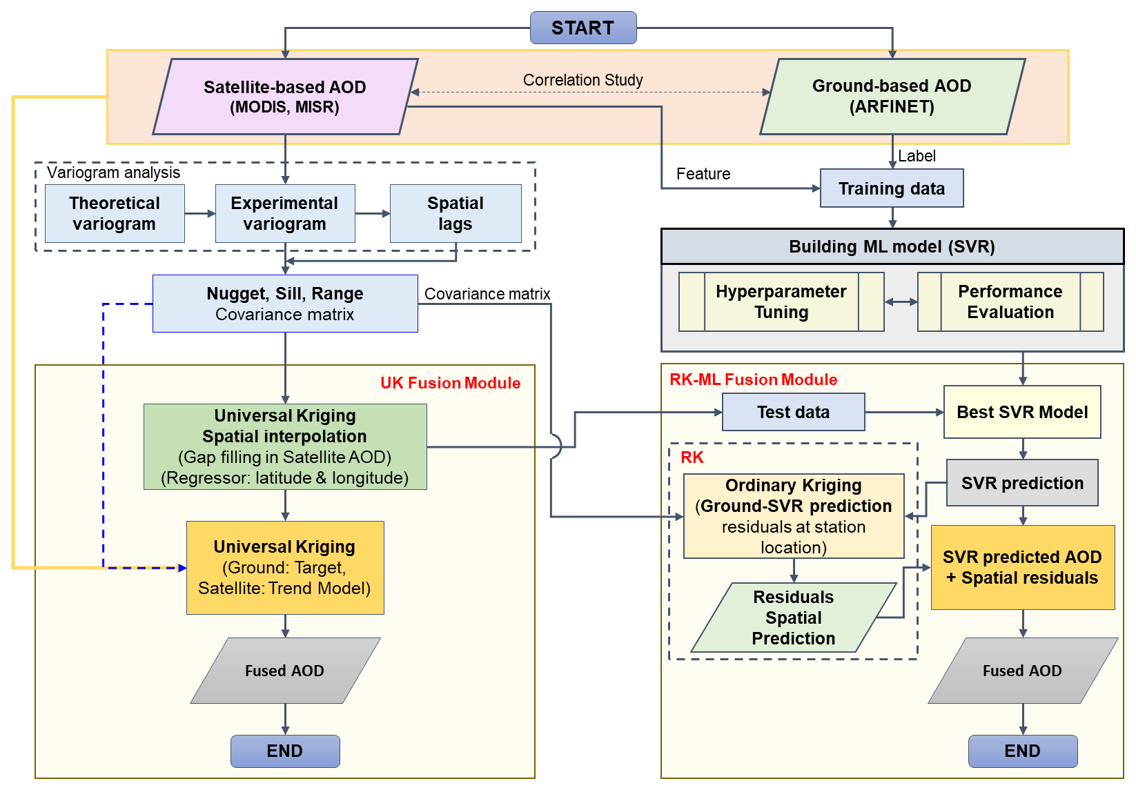
Figure 1 Flowchart of fusion methodology: Universal Kriging (UK) and Residual Kriging – Machine Learning (RK-ML). The machine learning best model is designed based on the long term MODIS and MISR data which were collocated with ground-based observations.

2.3 Fusion Methodology

The geostatistical data fusion method used in this study combines spatial data from multiple sources (satellite and ground-based, as detailed in Sect. 2.1 and 2.2) with varying resolutions, accuracies, and types of measurements. The aim is to enhance the overall understanding and prediction of spatial variables (e.g., AOD) to produce a more accurate and comprehensive representation of columnar AOD, with an emphasis on reducing inter-sensor biases through integration with ground-based observations. For this, we have adapted UK framework, where data interpolation relies on unknown functions (e.g., satellite derived AOD) represented as trend models with spatial autocorrelation through variogram analysis. Building on this framework, the fusion methodology is designed to operate under practical observational constraints, such as differences in sensor characteristics (e.g., spatial coverage, revisit frequency, and collocation with ground observations), which limit consistent data availability at daily timescales. Hence, the analysis is conducted at the monthly scale to improve spatial representativeness, reduce sampling gaps, and enhance statistical robustness. Notably, the monthly satellite AOD products also retain sensor-specific biases and inter-product inconsistencies. Thus, the fusion approach presented here is not primarily aimed at gap-filling, but at generating a more accurate and internally consistent AOD dataset by integrating complementary information from multiple sensors and ground-based observations. Thus, even at the monthly scale, the proposed method adds value by reducing retrieval uncertainties and improving the reliability of aerosol distributions, which is critical for climate studies and radiative forcing assessments. The overview of the fusion method is presented in Fig. 1, followed by a detailed description of each step in the following sections.

2.3.1 Correlation Analysis

As a first step of the fusion processes, the correlation analysis between the satellite and ground-based AOD was made to understand the association/biases between the two data sets at different spatiotemporal scales. This is useful to understand the requirement of multi-sensor data fusion. For this, a statistical spatio-temporal matching approach similar to those reported elsewhere by Basart et al. (2009). Chu et al. (2002), Filonchyk et al. (2019), Ichoku et al. (2002) was applied, in which satellite observations were spatially averaged at 0.5° spatial resolution and compared with ground-based AOD averaged within a 30 min time window around the overpass time of the TERRA satellite which accommodated 14 to 15 measurements from MWR (data frequency 2 min) and 1 to 2 measurements from CIMEL (data frequency 15 min) observations. Although satellite products such as MODIS (∼ 10 km) and MISR (∼ 4.4 km) provide higher spatial resolution potentially capturing finer regional variability in aerosol distributions, yet their direct comparison with ground-based point measurements introduces representativeness errors due to scale mismatch. Aggregating the data to a coarser grid (0.5°) reduces this mismatch by ensuring that both satellite and ground observations represent comparable spatial scales, thereby improving the robustness of validation and fusion. Thus, the choice of 0.5° represents an optimal choice, yielding higher correlation and lower root mean square error (RMSE) (Figs. S3 and S4), in addition to retaining regional variability and ensuring sufficient data density within each grid cell for stable statistical estimation and fusion. The consideration of 0.5° resolution is in line with approach adopted by Tandule et al. (2026) for retrieving AOD from satellite observations, ensuring improved representativeness and temporal consistency in comparisons between satellite-derived and ground-based AOD. In addition, generating AOD at this resolution provides a valuable reference dataset for comparison and validation against reanalysis products and model outputs of AOD, where satellite observations are commonly assimilated as primary inputs. Due to the differences in spatial coverage and revisit characteristics of MODIS and MISR as well as temporal gaps in data availability from ground-based instruments (Figs. S5–S7), daily datasets often contained substantial spatial gaps over the study domain. Therefore, AOD observations in this study were aggregated to a monthly scale to ensure more consistent spatial coverage and improve the reliability of multi-sensor fusion analysis.

2.3.2 Variogram Modeling

Variogram analysis is used to quantify and model the spatial autocorrelation (i.e., spatial dependence) of a dataset. It evaluates how the spatial variability between data points changes as a function of lag distance, the distance separating two sample points in space. To capture the spatial dependency of the data, geographical parameters such as latitude, longitude, and elevation are often incorporated as covariates in the trend function, thereby incorporating the spatial context of the sampling locations. This approach has been widely applied in studies involving meteorological parameters (Chua and Bras, 1982; Holdaway, 1996; Nalder and Wein, 1998). In the present context, spatial representation of AOD is fairly represented as a trend function comprising of latitude, longitude, and elevation, which serve as proxies for underlying spatial variations of geographical and atmospheric influences that significantly affect aerosol distribution. However, it is important to note that most geostatistical methods, such as Kriging, assume the underlying field to follow second order or, intrinsic stationarity (mean is constant, and the covariance or, variance of increments depends only on spatial lag). However, real-world environmental and geophysical data often exhibit large-scale spatial trends driven by physical and geographical factors, such as latitude, longitude, and elevation. In the case of AOD, these variables act as key spatial predictors that capture dominant regional gradients and can be used to model and remove the large-scale spatial trend. In the presence of strong spatial trends, variogram may become unbounded or exhibit unrealistically large ranges. These spatial trends violate the stationarity assumption which can lead to unbounded variogram. To address this spatial detrending of the data is performed, which isolates the local fluctuations or residuals from the spatial data set. This serves as an essential step in geostatistical analysis to ensure a well-defined and bounded variogram, enabling reliable estimation of sill, nugget, and range parameters for spatial covariance modeling. To validate this assumption, we obtained the frequency distribution of satellite AOD and their residuals (Fig. S8) after detrending. A nearly symmetric histogram of detrended residuals indicates that the trend component has been effectively removed, which is a prerequisite for second-order stationarity (Tang et al., 2016). Since the detrending in our study is purely a spatial operation, the temporal dimension is not explicitly considered and is effectively treated as constant during the detrending process. Consequently, the approach does not involve long-term datasets or explicitly account for seasonal variability.

The semivariance, which measures the degree of spatial variability between pairs of sample points as a function of their separation distance, known as the lag-distance (h), is calculated as:

$$\begin{array}{}\text{(4)}& \mathit{\gamma }\left(h_x\right)=\left(\mathrm{1}/\mathrm{2}n\left(h\right)\right)\left(\sum \left[z\right(x_i)-z(x_i+h){]}^{\mathrm{2}}\right)\end{array}$$

where z(x_i) and z(x_i+h) are the values of the variables of interest at locations x_i and x_i+h (= x_j), respectively; n(h) is the number of pairs of points separated by the lag-distance h, which is given as:

$$\begin{array}{}\text{(5)}& h_x=r{\cos }^{-\mathrm{1}}(\sin {\mathit{\phi }}_i\sin {\mathit{\phi }}_j-\cos {\mathit{\phi }}_i\cos {\mathit{\phi }}_j\cos ({\mathit{\theta }}_i-{\mathit{\theta }}_j\left)\right)\end{array}$$

where φ_i,j represent longitudes of locations x_i and x_j, and θ_i,j represent latitudes of locations x_i and x_j; r is the mean radius of the earth. Following this, the empirical variogram is calculated from the actual observational data, showing the relationship between semivariance and lag distance for each set of observations. The experimental variogram is obtained after binning semivariance at certain lags of the empirical variogram. The experimental variogram is then fitted with a theoretical model to describe the spatial continuity of the variable. The theoretical models considered in the present study include Exponential, Spherical, and Matheron models; the mathematical expressions are given as:

$$\begin{array}{}\text{(6)}& {\displaystyle }\begin{array}{rl}& {\mathit{\gamma }}_{\text{theo}}\left(h_x\right)\\ & =\left\{\begin{array}{ll}\mathrm{0}& h_x=\mathrm{0};\\ {\mathit{\sigma }}_{\mathrm{n}}^{\mathrm{2}}+{\mathit{\sigma }}_{\mathrm{b}}^{\mathrm{2}}(\mathrm{1}-\exp (-h_x/l\left)\right)& h_x>\mathrm{0};\end{array}\right.\text{(Exponential)}\end{array}\text{(7)}& {\displaystyle }\begin{array}{rl}& {\mathit{\gamma }}_{\text{theo}}\left(h_x\right)\\ & =\left\{\begin{array}{ll}\mathrm{0}& h_x=\mathrm{0};\\ {\mathit{\sigma }}_{\mathrm{n}}^{\mathrm{2}}+{\mathit{\sigma }}_{\mathrm{b}}^{\mathrm{2}}\left(\mathrm{3}{h}_x/\mathrm{2}l-\mathrm{1}{h}_x^{\mathrm{3}}/\mathrm{2}{l}^{\mathrm{3}}\right)& \mathrm{0}<h_x\le l;\\ {\mathit{\sigma }}_{\mathrm{n}}^{\mathrm{2}}+{\mathit{\sigma }}_{\mathrm{b}}^{\mathrm{2}}& h_x>l;\end{array}\right.\text{(Spherical)}\end{array}\text{(8)}& {\displaystyle }\begin{array}{rl}& {\mathit{\gamma }}_{\text{theo}}\left(h_x\right)\\ & =\left\{\begin{array}{ll}\mathrm{0}& h_x=\mathrm{0};\\ {\mathit{\sigma }}_{\mathrm{n}}^{\mathrm{2}}+{\mathit{\sigma }}_{\mathrm{b}}^{\mathrm{2}}\left(\mathrm{1}-\exp \left(-h_x^{\mathrm{2}}/l^{\mathrm{2}}\right)\right)& h_x>\mathrm{0};\end{array}\right.\text{(Matheron)}\end{array}\end{array}$$

In the above equations, ${\mathit{\sigma }}^{\mathrm{2}}={\mathit{\sigma }}_{\mathrm{n}}^{\mathrm{2}}+{\mathit{\sigma }}_{\mathrm{b}}^{\mathrm{2}}$, represents the total variance observed in AOD data at larger lag distances (spatially uncorrelated AOD data). ${\mathit{\sigma }}_{\mathrm{n}}^{\mathrm{2}}$ is nugget (y-intercept of the variogram), which represents the semivariance at a very small lag distance, approaching zero. Nugget (spatial variation at distances smaller than the smallest sampling interval) is indicative of the presence of measurement error or noise in the data. A large nugget relative to the sill (i.e., the semivariance value where the variogram levels off, representing maximum variability or correlation between data points at a given spatial distance) suggests significant measurement error or unresolved variability. This can indicate potential issues with data quality for spatial analysis. On the other hand, a small nugget implies that the data is relatively free of noise and that most of the spatial variability is due to the structured spatial process. ${\mathit{\sigma }}_{\mathrm{b}}^{\mathrm{2}}$ is variance in spatially correlated data, and this parameter gradually increases with increasing lag distances until it reaches sill. l is the range parameter, which controls the spatial autocorrelation length scale. It represents the distance over which data remain spatially correlated; beyond this distance, the semivariance approaches the sill. The higher the range, the more similar the values are at greater distances from each other. The spatial covariance function can be derived from the variogram model as:

$$\begin{array}{}\text{(9)}& C_{ij}={\mathit{\sigma }}^{\mathrm{2}}-{\mathit{\gamma }}_{\text{theo}}\end{array}$$

2.3.3 Universal Kriging

Universal Kriging (UK) also referred to as Kriging with a trend model, extends Ordinary Kriging by incorporating a deterministic trend component alongside the stochastic spatial component. This approach is useful when there is an underlying trend in the data that varies across the study area. The UK method uses both the spatial autocorrelation structure and the deterministic trend to make predictions. The UK model can be expressed as:

$$\begin{array}{}\text{(10)}& Z=M_{\mathrm{z}}\mathit{\beta }+\in \text{ \hspace{0.17em}\hspace{0.17em}\hspace{0.17em}\hspace{0.17em}\hspace{0.17em}\hspace{0.17em}Or},\in =Z-M_{\mathrm{z}}\mathit{\beta }\end{array}$$

where, $Z=\left[Z\right(x_{\mathrm{1}}),Z(x_{\mathrm{2}}),\mathrm{\dots }\mathrm{\dots },Z(x_{\mathrm{n}}){]}^{\mathrm{T}}$ represent the values of the variables of interest at locations $x_{\mathrm{1}},x_{\mathrm{2}},\mathrm{\dots }\mathrm{\dots },x_{\mathrm{n}}$, respectively. M_z is the deterministic trend component of the model (n×p) where p is representing the number of regressors; and β is the unknown drift coefficient (p×1) to be estimated; ∈ is the stochastic component or stochastic residuals (n×1), i.e., mean zero random fields.

In the present study, the trend component M_z for fusion is defined as

$$\begin{array}{}\text{(11)}& M_{\mathrm{z}}=\left(\begin{array}{lll}\mathrm{1}& {\text{MODIS}}_{{\text{AOD}}_{\mathrm{1}}}& {\text{MISR}}_{{\text{AOD}}_{\mathrm{1}}}\\ \mathrm{1}& {\text{MODIS}}_{{\text{AOD}}_{\mathrm{2}}}& {\text{MISR}}_{{\text{AOD}}_{\mathrm{2}}}\\ \mathrm{⋮}& \mathrm{⋮}& \mathrm{⋮}\\ \mathrm{1}& {\text{MODIS}}_{{\text{AOD}}_{\mathrm{n}}}& {\text{MISR}}_{{\text{AOD}}_{\mathrm{n}}}\end{array}\right)\end{array}$$

This is similar to a multiple regression model, which is described through a combination of a constant term and two sensor measurements that act as regressors to predict AOD at estimation locations. The first component of this trend model represents the overall offset (i.e., the mean of the portion of the AOD distribution that is not captured by MISR and MODIS). This constant term thereby represents any systematic offset between the combined (MISR and MODIS) satellite-retrieved AOD and the ground-measured AOD.

Following Eq. (10), the expected value at prediction locations (x_s) can be expressed as the best linear unbiased prediction (BLUP):

$$\begin{array}{}\text{(12)}& \widehat{Z}\left(x_{\mathrm{s}}\right)=m_s^{\mathrm{T}}\widehat{\mathit{\beta }}+{\mathbf{C}}_{\text{zs}}^{\mathrm{T}}{\mathbf{C}}_{\text{zz}}^{-\mathrm{1}}\left(Z-M_{\mathrm{z}}\widehat{\mathit{\beta }}\right)\end{array}$$

Here, C_zs(n×s) is the spatial covariance matrix of the residuals between the sample location (i.e., measurement locations) and prediction locations (i.e., estimation locations) and C_zz(n×n) is the spatial covariance matrix of the residuals between the sample locations (i.e., measurement locations) as obtained from Eq. (9). The unknown coefficient $\widehat{\mathit{\beta }}$ can be expressed as the generalized least squares (GLS) estimator from the covariance matrix,

$$\begin{array}{}\text{(13)}& \widehat{\mathit{\beta }}={\left(M_{\mathrm{z}}^{\mathrm{T}}{\mathbf{C}}_{\text{zz}}^{-\mathrm{1}}{M}_{\mathrm{z}}\right)}^{-\mathrm{1}}{M}_{\mathrm{z}}^{\mathrm{T}}{\mathbf{C}}_{\text{zz}}^{-\mathrm{1}}Z\end{array}$$

Alternatively, minimizing the mean square error (MSE) of all predictions among the predictors of the form λ^TZ subjected to unbiasedness constraint, i.e., E(λ^TZ)=E(Z(x_s)) for all β, which is identical to ${\mathit{\lambda }}^{\mathrm{T}}{M}_{\mathrm{z}}\widehat{\mathit{\beta }}=m_s^{\mathrm{T}}\widehat{\mathit{\beta }}$ and under conditions for minimizing variance (λ^TZ−Z), Lagrange multipliers μ(n×s) are used to solve the linear constraint equations as given below,

$$\begin{array}{}\text{(14)}& \left[\begin{array}{cc}{\mathbf{C}}_{\text{zz}}& M_{\mathrm{z}}\\ M_{\mathrm{z}}^{\mathrm{T}}& \mathrm{0}\end{array}\right]\left[\begin{array}{c}\mathit{\lambda }\\ \mathit{\mu }\end{array}\right]=\left[\begin{array}{c}{\mathbf{C}}_{\text{zs}}\\ m_s\end{array}\right]\end{array}$$

Here, M_z(n×p) and $M_{\mathrm{z}}^{\mathrm{T}}(p\times n)$ are trend models of AOD given by Eq. (11); m_s(p×s) is trend model at s estimation locations; λ(n×s) are the Kriging weights, μ is the Lagrange multiplier.

The system of equations is solved for Lagrange multiplier μ and weights λ to estimate AOD at estimation locations. This can be expressed as:

$$\begin{array}{}\text{(15)}& {\displaystyle }\left[\begin{array}{c}\mathit{\lambda }\\ \mathit{\mu }\end{array}\right]={\left[\begin{array}{cc}{\mathbf{C}}_{\text{zz}}& M_{\mathrm{z}}\\ M_{\mathrm{z}}^{\mathrm{T}}& \mathrm{0}\end{array}\right]}^{-\mathrm{1}}\left[\begin{array}{c}{\mathbf{C}}_{\text{zs}}\\ m_s\end{array}\right]\text{(16)}& {\displaystyle }\begin{array}{rl}\mathit{\lambda }=& \left\{{\mathbf{C}}_{\text{zz}}^{-\mathrm{1}}-{\mathbf{C}}_{\text{zz}}^{-\mathrm{1}}{M}_{\mathrm{z}}{\left(M_{\mathrm{z}}^{\mathrm{T}}{\mathbf{C}}_{\text{zz}}^{-\mathrm{1}}{M}_{\mathrm{z}}\right)}^{-\mathrm{1}}{M}_{\mathrm{z}}^{\mathrm{T}}{\mathbf{C}}_{\text{zz}}^{-\mathrm{1}}\right\}{\mathbf{C}}_{\text{zs}}\\ & +{\mathbf{C}}_{\text{zz}}^{-\mathrm{1}}{M}_{\mathrm{z}}{\left(M_{\mathrm{z}}^{\mathrm{T}}{\mathbf{C}}_{\text{zz}}^{-\mathrm{1}}{M}_{\mathrm{z}}\right)}^{-\mathrm{1}}{m}_s\end{array}\text{(17)}& {\displaystyle }{\mathit{\lambda }}^{\mathrm{T}}Z={\mathbf{C}}_{\text{zs}}^{\text{T}}{\mathbf{C}}_{\text{zz}}^{-\mathrm{1}}(Z-M_{\mathrm{z}}\mathit{\beta })+m_s^{\mathrm{T}}\mathit{\beta }\end{array}$$

The prediction variance associated with predicted values can be represented as

$$\begin{array}{}\text{(18)}& \begin{array}{rl}& \text{Var}\left(Z\left(x_{\mathrm{s}}\right)-\widehat{Z}\left(x_{\mathrm{s}}\right)\right)\\ & ={\mathit{\sigma }}_{Z\left(x_{\mathrm{s}}\right)}^{\mathrm{2}}-{\mathbf{C}}_{\text{zs}}^{\text{T}}{\mathbf{C}}_{\text{zz}}^{-\mathrm{1}}{C}_{\text{zs}}+{\left(m_s^{\mathrm{T}}-{\left(M_{\mathrm{z}}^{\mathrm{T}}{\mathbf{C}}_{\text{zz}}^{-\mathrm{1}}{\mathbf{C}}_{\text{zs}}\right)}^{\mathrm{T}}\right)}^{\mathrm{T}}\\ & \times {\left(M_{\mathrm{z}}^{\mathrm{T}}{\mathbf{C}}_{\text{zz}}^{-\mathrm{1}}{M}_{\mathrm{z}}\right)}^{-\mathrm{1}}\left(m_s^{\mathrm{T}}-{\left(M_{\mathrm{z}}^{\mathrm{T}}{\mathbf{C}}_{\text{zz}}^{-\mathrm{1}}{\mathbf{C}}_{\text{zs}}\right)}^{\mathrm{T}}\right)\end{array}\end{array}$$

The above weighting approach determines the values at prediction locations. Our foremost approach involved creating a trend model for fusion. For this purpose, we generated a complete satellite-based map of AOD from MODIS and MISR separately over the study region using the UK method. In this framework, geographical parameters such as latitude, longitude and elevation are treated as regressors (trend model), whereas observed satellite data serve as response variables to fill the gaps in individual satellite datasets. Subsequently, in the final spatial fused predictions, the ground-based AODs were treated as the response variables, where the satellite data, along with the elevation model (used as additional information), were used as regressors.

2.3.4 Residual Kriging – Machine Learning (RK-ML)

The RK-ML approach is implemented in this study through a hybrid approach to generate reliable estimates of fused AOD, with improved predictive accuracy using a limited number of ground-based observations. Although UK and the proposed RK-ML approach appear methodologically different, they share a common conceptual foundation. From a generalized regression perspective, both methods rely on a covariance structure to characterize spatial dependence among grid points. However, when the number of observations is limited, the statistical parameters in UK can adversely affect predictions at estimation locations. To overcome the limitations associated with limited observations, SVR is employed due to robustness of its regularized formulation in both regression and classification tasks (Sifaou et al., 2021), where predictions are learned from datasets within a historical training window. These predictions provide prior information on ground-based AOD that is independent of the spatial configuration of the current ground based-observations.

The best-performing SVR model is first identified based on a time window of five years of data (simultaneous MODIS, MISR and ground measurements) for a specific month (season) targeting consistent aerosol conditions. Subsequently, this model leverages spatially interpolated features from MODIS and MISR data (gap filled AOD by UK) to generate SVR-predicted maps to obtain a full generalized AOD map for that month. The discrepancies between SVR-predicted values and observed ground measurements are treated as residuals, which are then spatially modeled using Ordinary Kriging. The resulting residual predictions are combined with SVR outputs to produce RK-ML-based fused products. This approach provides a robust alternative to traditional UK-based data fusion techniques by capturing complex relationships between predictors and target variables. The detailed RK-ML methodology is given below.

SVR transforms features into a higher-dimensional space, making them linearly separable and helps improving the prediction of target variables like ground based AOD. The use of SVR in Kriging has been reported in previous studies to improve model predictions (Wang et al., 2008; Baisad et al., 2023). The SVR model is represented by:

$$\begin{array}{}\text{(19)}& Z_{\text{svr}}=w^{\mathrm{T}}\mathit{\phi }+b\end{array}$$

where φ is the kernel transformed input features, w is the nonzero vector normal to hyperplane (the plane or decision boundary that best fits the n dimension input vectors while maintaining a margin of tolerance (ε-insensitive zone) around it) and bϵR. This expression assumes that Z_svr exist when it approximates all w^Tφ with ε precision for linearly separable data. Along with it, the concept of soft margin loss function is considered which introduces slack variable ξ(+ve) and ${\mathit{\xi }}^{\ast }(-\text{ve})$ to allow some points lying inside the hyperplane.

Hence the optimization problem is subject to minimization of

$$\begin{array}{}\text{(20)}& \begin{array}{rl}& {\displaystyle \frac{\mathrm{1}}{\mathrm{2}}}{∥w∥}^{\mathrm{2}}+C{\sum }_{i=\mathrm{1}}^l(\mathit{\xi }+{\mathit{\xi }}^{\ast })\\ & \text{Such that }\left\{\begin{array}{l}Z-w^{\mathrm{T}}\mathit{\phi }-b\le \mathit{\epsilon }+\mathit{\xi }\\ w^{\mathrm{T}}\mathit{\phi }+b-Z\ge \mathit{\epsilon }+{\mathit{\xi }}^{\ast }\\ {\mathit{\xi }}_i{\mathit{\xi }}_i^{\ast }\ge \mathrm{0}\end{array}\right.\end{array}\end{array}$$

The regularization constant C trades off between the model complexity and empirical error up to which deviations larger than ε can be tolerated. $\mathit{\xi },{\mathit{\xi }}^{\ast }$ are regression errors. The detailed explanation of SVR model is available in the literature (Smola and Schölkopf, 2004; Brereton and Lloyd, 2010; Zhang and O'Donnell, 2020). In the present study, best model of SVR is decided from the minimum RMSE between predicted AOD and observed AOD after tuning its hyperparameters.

The residuals, which are the difference between collocated AOD of SVR predictions from ground based AOD, are estimated from the difference between ${\widehat{Z}}_{\text{svr}}\left(x_{\mathrm{s}}\right)$ and Z, i.e., ${\widehat{Z}}_{\text{svr}}\left(x_{\mathrm{s}}\right)-Z$. These residuals under ordinary Kriging are modeled as $\mathit{\delta }\left(s\right)=\mathit{\mu }+\mathit{\epsilon }\left(s\right)$ where μ refers to the mean values of residuals over study domain, which resembles similar mathematics of universal Kriging, except M_z and m_s=1 (Eqs. 10 to 17). Following this, the estimated residuals at unknown locations are determined as δ(x_s)=λ^Tδ(x_z).

The weighting parameter λ is obtained from the covariance matrices as follows

$$\begin{array}{}\text{(21)}& \left[\begin{array}{c}\mathit{\lambda }\\ \mathit{\mu }\end{array}\right]={\left[\begin{array}{cc}{\mathbf{C}}_{\text{zz}}& \mathrm{1}\\ \mathrm{1}& \mathrm{0}\end{array}\right]}^{-\mathrm{1}}\left[\begin{array}{c}{\mathbf{C}}_{\text{zs}}\\ \mathrm{1}\end{array}\right]\end{array}$$

The ordinary Kriging estimation contains the spatial relation while the SVR prediction contains the optimal estimations from features (Satellite) and labels (Ground AOD). The final fused map can then be estimated as

$$\begin{array}{}\text{(22)}& Z=\mathit{\delta }\left(x_{\mathrm{s}}\right)+Z_{\text{svr}}\left(x_{\mathrm{s}}\right)\end{array}$$

The hyperparameters of the SVR model were optimized using a grid-search strategy as part of the training process. In this approach, predefined values for key hyperparameters – such as the regularization parameter (C), kernel type, gamma (Υ) and epsilon (ε) – were combined to form all possible parameter configurations, and each configuration was evaluated. For every hyperparameter combination, model performance was assessed using the negative mean squared error (neg-MSE) as the evaluation metric. This metric quantifies prediction error, and allows selection of the best model by maximizing the score. Due to the limited size of the dataset, leave-one-out cross-validation (LOOCV) was used during training instead of k-fold cross-validation. Even though other cross-validation approaches, such as site-based, temporal, or sample-based validation, can also be used to assess model robustness, the LOOCV was considered the most suitable approach in this study considering the limited number of samples and the uneven spatial distribution of ground observations. In LOOCV, the model is trained repeatedly on all samples except one, which is used for validation. This procedure is repeated so that each data point serves once as a validation sample. This approach maximized the use of available data while providing an unbiased estimate of model performance. Based on this procedure, a linear kernel was identified as the optimal choice for the RK-ML models, which were subsequently evaluated on independent test sets (20 % for MODIS, N = 318; 10 % for MISR, N = 71). For MODIS AOD features, the best model configuration was C=1, gamma = “scale”, kernel = “linear”; for MISR AOD features, the optimal configuration was C=100, gamma = “scale”, kernel = “linear”. The use of a linear kernel suggests a predominantly linear relationship between satellite observations and ground-based AOD. Inclusion of the regularization parameters C and gamma controls overfitting and penalizes noisy inputs, enabling the ML framework to generate more reliable estimates. These estimates were further corrected using spatial residuals from RK, allowing RK-ML to outperform UK under conditions of limited or biased AOD observations. The final models were evaluated using correlation coefficient (R), R², mean absolute error (MAE), and RMSE on both training and test sets (Table S1 in the Supplement). Results indicate that training and test performances were comparable (with training R² values either lower or close to test R²), correlation coefficients were consistently high, and errors (RMSE, MAE) were low. These outcomes confirm that the SVR models did not suffer from overfitting and generalized well to unseen data, despite the limited sample size. Although other machine learning algorithms, such as Random Forest (RF) and XGBoost, can also be integrated within the RK-ML framework, a sensitivity analysis conducted on MODIS test dataset indicated that SVR achieved comparable or better performance metrics (R, RMSE; Fig. S9).

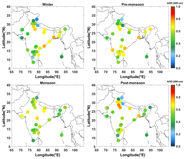
Figure 2 Long-term (2011–2020) ground-based AOD at 500 nm from MWR and MICROTOPS-II sunphotometer measurements in the ARFINET over the Indian region. The seasons are winter: December, January, February (DJF); Pre-monsoon: March, April, May (MAM); Monsoon: June, July, August, September (JJAS); Post-monsoon: October, November (ON). The different regions considered for representing Indo–Gangetic plane (IGP), North-west (NW), North-east (NE), Peninsular India (PI), and Central India (CI) are provided (Fig. S10).

3 Results and Discussions

3.1 Regional distribution of AOD from ground- and satellite-based observations

The analysis of spatial distribution of AOD is crucial for understanding the consistency of measurements across different sensors. The large-scale spatial variations in the data help identifying overall spatial trends over latitude-longitude and geographic elevation. Emphasizing spatial trends is also critical for assessing the mathematical assumptions underlying Kriging and variogram analysis, which rely on the condition of second-order stationarity within the sampled data. In view of this, ground-based AOD at 500 nm was considered for long-term comparison of MODIS and MISR AOD at 550 nm as the closest approximation. The typical AOD patterns over different regions over India, derived from 10 years of ground-based MWR and MICROTOPS-II sunphotometer measurements in the ARFINET, is illustrated in Fig. 2.

Various factors such as the relative dominance of natural and anthropogenic sources, local and synoptic meteorology cause observed spatio-temporal variations in AOD at a particular location. Over most of the locations in the Indo-Gangetic Plains (IGP), AOD shows consistent high values (> 0.6) throughout different seasons. This is similar to the observations reported by Lodhi et al. (2013), Singh et al. (2020), Tiwari et al. (2018). Next to the IGP, the north-eastern (NE) India experiences higher AOD with peak during the pre-monsoon season. Similar pattern is reported elsewhere (Gogoi et al., 2009). In Peninsular India (PI), AOD is highest during the pre-monsoon period, followed by a significant reduction during the summer monsoon. This is similar to the earlier studies by Kalluri et al. (2016), Kumar et al. (2009), Sinha et al. (2013), Viswanatha et al. (2018).

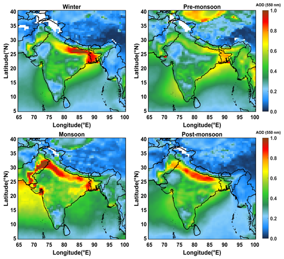
Figure 3 Long-term (2011–2020) satellite-based AOD (at 550 nm) from MODIS over south-Asian region.

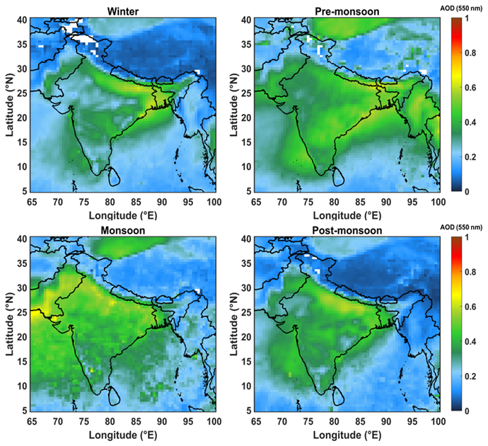
Figure 4 Similar analysis as in Fig. 3 but for MISR.

The spatial patterns of a decadal average (2011–2020) satellite-based MODIS and MISR AOD (Figs. 3 and 4) also shows persistent high AOD values in the IGP and its outflow regions across all seasons. In PI, the presence of elevated mountain ranges such as the Western and Eastern Ghats, coupled with its proximity to the Indian Ocean, results in regional-scale AOD variability. During the pre-monsoon and monsoon periods, oceanic and coastal regions exhibit higher AOD levels compared to the winter and post-monsoon periods. Though dominant spatial patterns are same in long term AOD from both space-borne sensors and their differences with ground-based AOD over same spatial grids are minimal, the discrepancy persists, especially over northern India and during monsoon period (Figs. S11 and S12). As cloud-haze misclassifications may act as one of the factors for the observed differences between satellite- and ground-based AOD in the monsoon periods, haze/cloud discrimination criteria following Jiao et al. (2023) was applied to MODIS AOD. A significant impact of haze over the peninsular region is seen during monsoon (Figs. S13 and S14), though it shows negligible influence during the other seasons. This is clearly seen from the difference maps between the MODIS and ground-AOD over different ground locations, showing minimal changes before and after the haze removal. This exercise suggests that cloud-haze misclassification is not the primary factor driving the observed differences, except under monsoon conditions. Under such a scenario, localized discrepancies may arise due to spatial sampling limitations of the ground-based observations. As the ARFINET stations are sparsely and unevenly distributed, particularly across regions of high aerosol loading in northern India, this may result in the apparent lack of complete regional representation of ground observations. Additionally, discrepancies between MODIS and MISR AOD are also seen owing to fixed and multi angle retrievals, especially in Pre-monsoon period over the NW region, where MISR AOD is significantly different from MODIS. There are also some pockets where low AOD region observed by MODIS is alternatively represented as a region of higher AOD in MISR observations, particularly in proximity to the IGP outflow. Previous studies over similar geographic regions have indicated that the frequency of observations, cloud masking, and geographical factors impact both MODIS and MISR observations, stemming from algorithm assumptions related to cloud masking and SSA. Overall, the spatial patterns of AOD from ground- and satellite-based observations reveal the following:

• During the pre-monsoon period, northern India experiences increased AOD.

• During the winter season, cold temperatures, a low boundary layer height, and humid air create hazy conditions with high AOD (Nair et al., 2020). Along with it, winds over the IGP are mostly north-westerly, with an anti-cyclonic pattern over central India, driving aerosols to peninsular region.

• The post-monsoon AOD also remains high, similar to winter levels, particularly in the IGP due to biomass burning (Kumar et al., 2012; Lodhi et al., 2013; Subba et al., 2022).

• The spatial patterns of AOD across different seasons are well captured by both ground- and satellite-based observations. However, notable differences exist between the two. While MODIS tends to overestimate AOD over the IGP, it generally underestimates AOD over the PI, NE, and NW regions. MISR significantly underestimates higher AOD regions.

Despite the above constraints, the general agreement in magnitude and temporal variability supports the reliability of both datasets for the fusion framework. Thus, our approach explicitly accounts for such discrepancies by integrating the broad spatial coverage of satellite observations with the higher accuracy of ground-based measurements. In this context, ground observations are treated as local constraints rather than complete spatial representations, thereby minimizing the regional sampling gaps in the ground network. Consequently, the final fused AOD represents a bias-corrected satellite-retrieved AOD constrained by ground observations.

3.2 Inter-comparison of satellite- and ground-based AOD

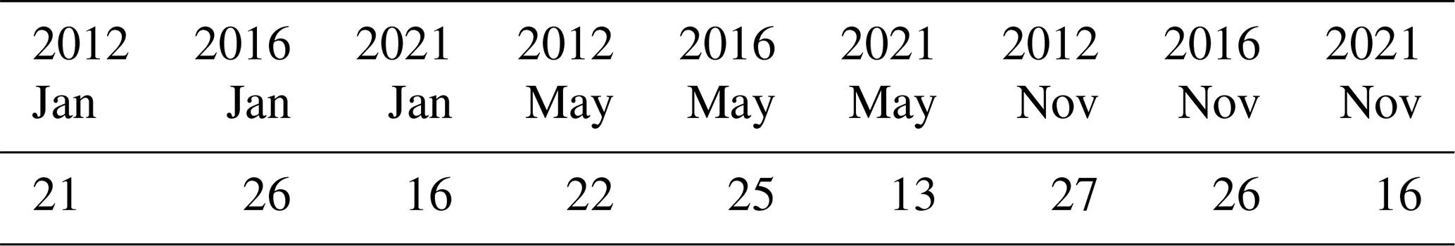
Having examined the spatial distribution, a quantitative evaluation of the associations or biases between satellite and ground-based AOD at different periods is carried out for the years 2012, 2016, and 2021. The three different years were selected such that way that the AOD for 2012 and 2021 provides the decadal variability, while 2016 represents an intermediate period between these two years, enabling us to better assess the progression and variability of AOD over a long period. The scatter plots (Figs. S15–S17; the number of ground stations included in the correlation studies is given in Table 1) between MODIS/ MISR and ground-based AOD highlight moderate to strong correlations (∼ 0.8–0.9) in winter (January) and post-monsoon (November), while moderate correlations (∼ 0.54–0.77) between the two are observed in pre-monsoon (May). The RMSE between MISR and ground-based AOD is higher (≥ 0.2) during winter and post-monsoon, whereas higher RMSE values between MODIS and ground-based AOD are observed during the pre-monsoon period. The prominent locations contributing to mean errors and weak correlations with ground observations are situated in the NW and IGP regions. The quartile-plots (Figs. S18–S20) clearly support these observations highlighting significant spatio-temporal variability in AOD, with both sensors displaying higher AOD over terrestrial regions, particularly in the IGP, its outflows, and South (Peninsular) and Central India. The third and fourth quartiles are more representative for AOD over land regions than in surrounding areas like oceans and elevated terrain. Data with respect to longitude and latitude show that higher AOD values are mostly confined to 20–30° N latitude and 80–95° E longitude. Notably, MODIS consistently recorded significantly higher AOD values than MISR, with notable dissimilarities in quartile patterns over northern India during May.

Table 1 Number of ground stations data used in different months of the year 2012, 2016, and 2021.

Both the correlation and quartile analyses highlight the advantages and limitations of MODIS and MISR observations. For example, MISR tends to underestimate high AOD conditions in urban regions compared to MODIS, even though it can effectively separate surface contributions under low aerosol loading, as also reported by Tao et al. (2020). Under high AOD conditions, the benefit of multi-angle measurements becomes limited, as thick aerosol layers smooth out surface reflectance signals, potentially leading to an underestimation of AOD due to misattribution of aerosol contributions to surface reflectance. In contrast, when dust loading is dominated by coarse and non-spherical particles (in May), MISR demonstrates enhanced sensitivity to aerosol microphysics, hence relatively better performance than MODIS (as shown by scatter plots). This difference may be attributed to the advantage of multi-angle observation capability of MISR, consistent with findings from Middle Eastern validation studies (Farahat, 2019; Garay et al., 2017).

3.3 Fusion of satellite- and ground-based AOD

3.3.1 Variogram Analysis

For the fusion of satellite- and ground-based AOD, the experimental variogram (using Eq. 2) is first obtained from the gridded satellite data. As mentioned in Sect. 2.3.2, a well-fitted variogram is essential for determining appropriate geostatistical parameters. Thus, the determination of variogram parameters like sill, range, and nugget are not unique but depend on the theoretical models used. The choice of fitting is determined through a least square approach, selecting the best fit based on the minimum of sum squared errors (SSE). However, the availability of a large number of satellite data sets has made this task easier. The variogram depicted in Figs. S21–S23 demonstrate a flattening of variance after a certain lag (interval between distances), affirming the effectiveness of our implemented detrending method. AOD values within the range highlight spatial correlation, wherein the correlated AOD values are influential in determining missing AOD values.

The variogram parameters obtained from the fitted theoretical model are given in Tables 2 and 3. The variogram parameters corresponding to different sensors exhibit noticeable variation across months and years, reflecting differences in their retrieval characteristics and ability to represent AOD. For instance, both MODIS and MISR AOD show shorter spatial correlation lengths and low sill values in May compared to January and November. Such reduced sill or, range values indicate the influence of long-range dust or smoke transport processes over some regions, which dominate during this period in the study region. Conversely, longer ranges indicate that the sensor retrievals capture more spatially homogeneous values, suggesting an improved ability to represent regional variability. In this study, we prioritize MODIS variogram because of their higher sill and range values, which demonstrate stronger spatial dependency (Isaaks and Srivastava, 1989; Vieira et al., 2009). Nevertheless, sensitivity tests indicate that using variogram derived from either MODIS or MISR produces only negligible differences (∼ 0.01) in the fused AOD estimates (Fig. S24). At this stage, it is also to be noted that geographically weighted or local variogram approaches can better represent spatial heterogeneity, particularly over complex terrains such as the Himalayas and Western Ghats. However, in the present study, this approach was not feasible due to the limited availability of ground-based AOD observations, especially across high-altitude regions. The sparse coverage restricts the stability and generalizability of local variogram fitting, particularly at regional boundaries where different models would be required. For this reason, we adopted a single variogram model, following the approach used for large regions (e.g., eastern and western USA; Chatterjee et al., 2010), which provides a more consistent framework for regional-scale fusion.

Table 2 Parameters obtained from variogram in different seasons (January, May, and November) of different years (2012, 2016, and 2021) from MODIS.

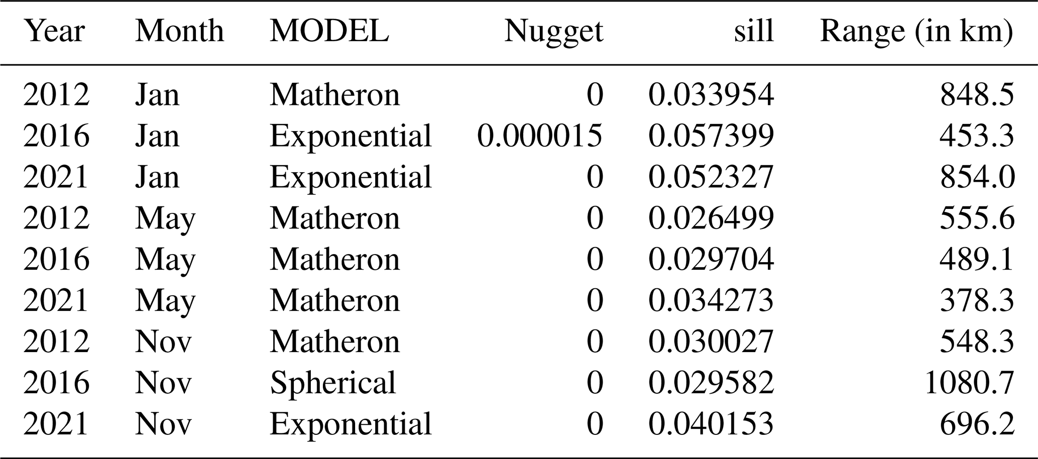
Table 3 Parameters obtained from variogram in different seasons (January, May, and November) of different years (2012, 2016, and 2021) from MISR.

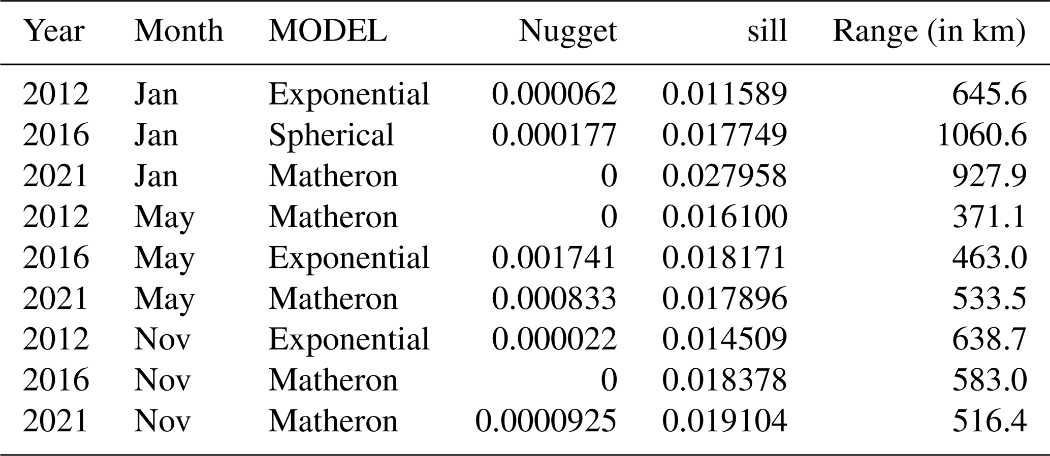
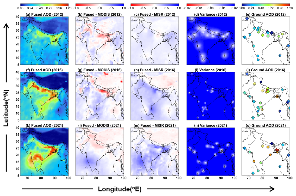
Figure 5 Monthly fused AOD (at 550 nm) maps (a, f, k) in January for the years 2012, 2016, 2021; (b, g, i, c, h, m) – the deviations of MODIS and MISR AOD from the corresponding fused AOD; (d, i, n) variance; and (e, j, o) – ground-based AOD (ARFINET is represented by circle and AERONET by diamond shapes) used to generate fused maps. Blue indicates overestimations, and red means an underestimation of fused AOD from satellite retrieved AOD. The white dots in variance plots show the ground station locations.

3.3.2 Spatial interpolation of AOD

Monthly mean AOD gives the advantage of having full regional picture of columnar aerosol load over south-Asian region. However, it is observed that both MODIS and MISR AOD show gaps in some of the regions, either due to consistent cloud coverage or due to complex orography coupled with highly reflective land masses (e.g., snow-covered regions of the Himalayas). Hence, UK with geographic parameters as regressors applied to fill these missing areas (which are found to be ∼ 2 %–11 %) to obtain a complete spatial picture of AOD over the south-Asian region. Kriging gives a probability map and the associated variance is higher in the gap regions than in the regions where values exist. Thus, the interpolated values and variances are not unique, as they depend on the variogram and trend models used in the interpolation. On the other hand, the variogram can have uncertainties that stem from factors such as lag spacing, the quantity of data points, and model fitting, as highlighted by researchers (Derakhshan and Leuangthong, 1982; Koushavand et al., 2008).

The spatial distribution of 0.5° gridded monthly mean raw and predicted (after spatial interpolation) AOD from MODIS and MISR is shown in Figs. S25–S30. The performance metrics (in terms of R and RMSE) of this gap-filling approach are demonstrated through sensitivity studies, considering different spatial gaps in the data (Fig. S31). It is observed that the predicted AOD largely depends on the availability and spatial distribution of nearby observed data points. Regions such as the IGP, the Himalayan region, peninsular India, and oceanic areas generally show better performance, where smoother spatial gradients of AOD and more consistent regional aerosol patterns improve the reliability of the spatial predictions. Based on these sensitivity studies, the predicted AOD field appears to provide a reliable spatial representation with acceptable uncertainty as the interpolation (gap filling) is made over a relatively small fraction of missing values based on a large number of observed data points around the gap areas. Overall, it is to be noted that, our proposed approach is not intended solely to enhance spatial coverage, but to generate a bias-corrected and internally consistent AOD dataset through the optimal integration of complementary satellite products.

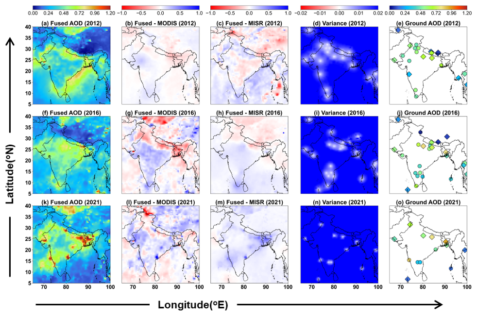
Figure 6 Similar analysis as in Fig. 5, but for the month of May in 2012, 2016, and 2021.

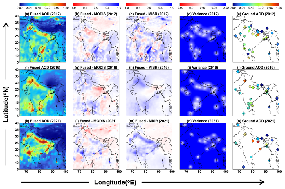
Figure 7 Similar analysis as in Fig. 5, but for the month of November in 2012, 2016, and 2021.

3.3.3 Fused AOD

The monthly fused AOD is generated using the UK fusion method, where satellite data are treated as trend model. This retains the overall spatial signatures of AOD from each satellite sensor. The optimal AOD values are determined by the weights obtained from spatial relationships, along with the trend of the satellite-based AOD at the estimation locations. Figures 5–7 show the fused maps of AOD at different seasons of the years 2012, 2016, and 2021. The regional average values of fused AOD, along with AOD from individual sensors, are given in Tables S4–S6.

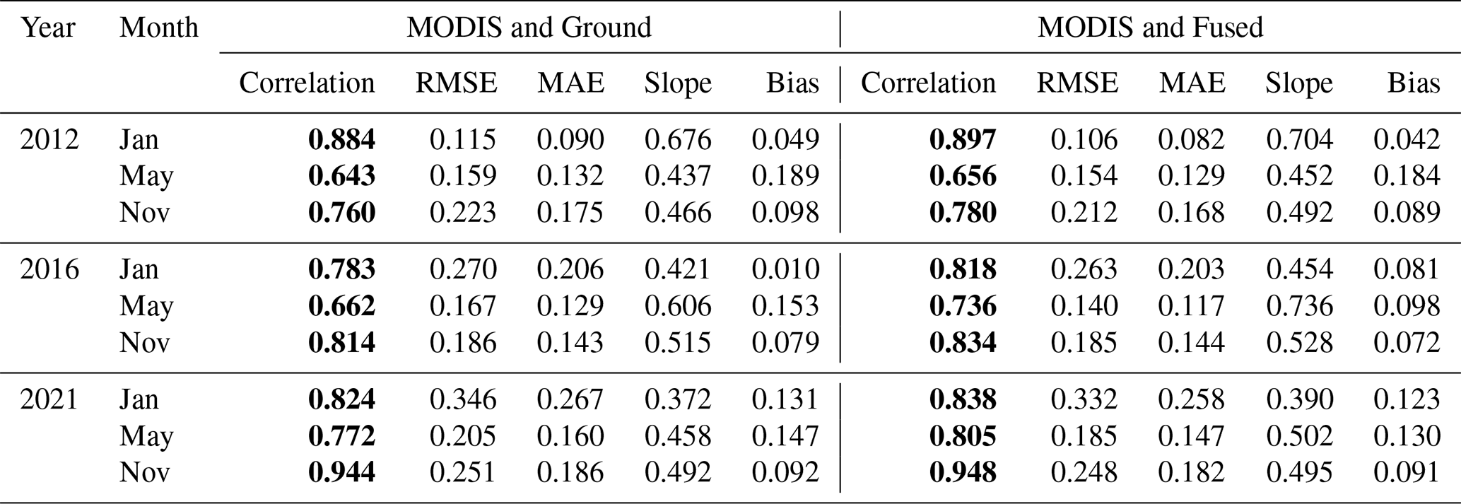
Throughout the observation period, the fusion maps highlight the significant influence of ground-based AOD. As shown in Table 4 (Figs. S32–S34), the fused AOD is more aligned to ground-based AOD with a correlation of R ∼ 0.994–1 and RMSE ∼ 0.009–0.04. On the other hand, correlation between MODIS/MISR and fused AOD shows little improvement compared to that between MODIS/MISR and ground-based AOD (Tables 5 and 6; Figs. S32–S34). This indicates the robustness of the fusion approach keeping ground-based AOD as an anchoring reference.

Table 4 Comparative analysis of ground-based vs. fused AOD at ground station locations. The values in bold indicate the prominent changes of the correlation coefficients after fusion.

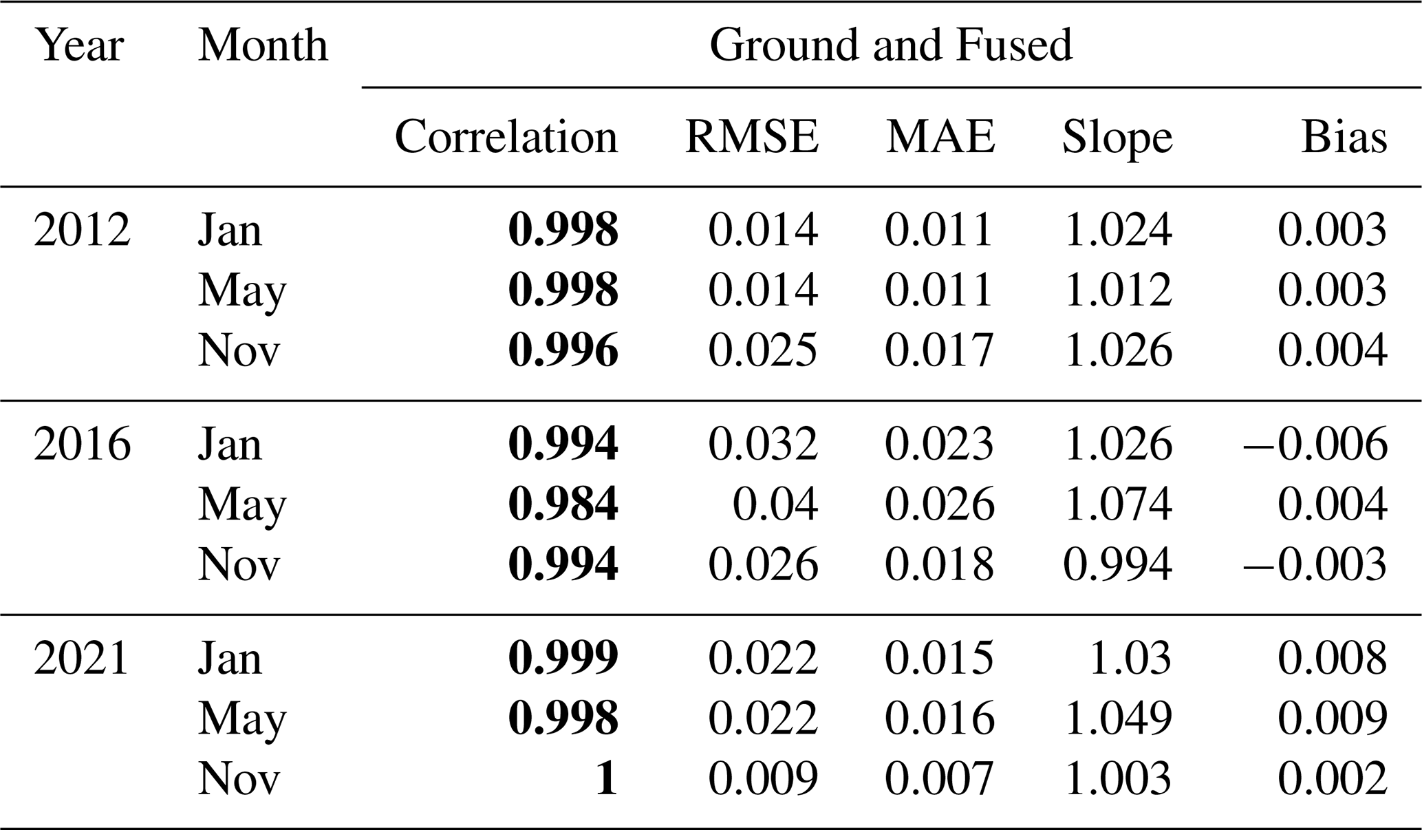
Table 5 Error and bias analysis of MODIS AOD with respect to ground and fused AOD at ground station locations. The values in bold indicate the prominent changes of the correlation coefficients before fusion and after fusion.

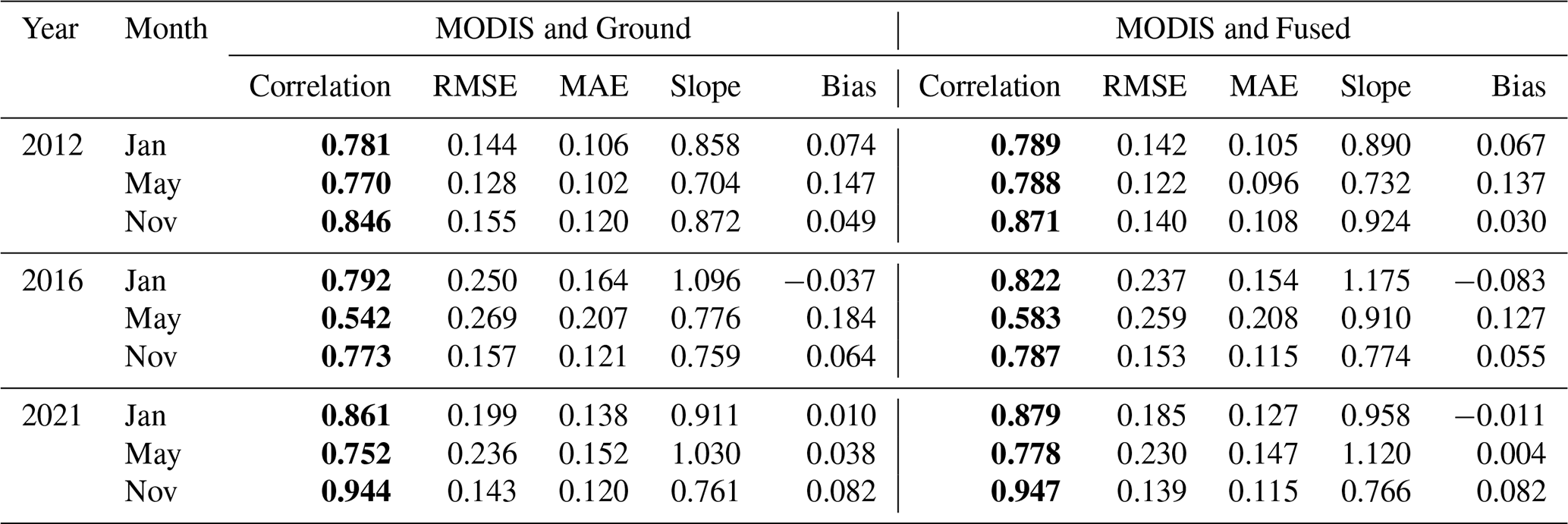
Table 6 Error and bias analysis of MISR AOD with respect to ground and fused AOD at ground station locations. The values in bold indicate the prominent changes of the correlation coefficients before fusion and after fusion.

The notable outcomes from fused AOD maps are the distinct spatial features compared to those obtained from individual space-based sensors. For example, during January 2016, the significant overestimation by MODIS (AOD ∼ 1.7) relative to ground-based AOD (∼ 1.2) is adjusted in the fused AOD distribution, thus correcting the bias but maintaining the spatial heterogeneity. Similarly, in January 2021, MODIS and MISR significantly underestimated AOD over peninsular India (MODIS AOD ∼ 0.36 and MISR AOD ∼ 0.30) as compared to ground AOD (e.g., AOD at GOA ∼ 0.95). The fused AOD corrects this bias toward values closer to ground-based observations, retaining continuous flow of aerosols toward the Arabian coast.

Similar observations are also evident during the pre-monsoon period. However, during this period, the fused AOD maps retain more of MISR spatial patterns in 2016 and 2021, while resembling MODIS in 2012. Notably, the discrepancies seen near coastal regions in May (2021), particularly across the peninsular zone, may be attributed to higher cloud fractions (Fig. S35), introducing greater uncertainty in aerosol–cloud discrimination (Lang et al., 2026), thereby leading to inaccuracies in satellite-derived AOD estimates. The fused AOD, which primarily incorporates the information from the availability and spatial proximity of ground-based measurements, effectively corrects this bias.

During the retreating monsoon season, the association of satellite and ground AOD is good, with similar spatial distribution over northern regions, while significant differences exists over southern parts. In the spatial map of fused AOD, the bias correction is clearly seen. In November 2016, over the NW and IGP, a significant bias correction in satellite AOD is observed, which is clearly indicated by the observed difference between fused AOD and satellite measurements. Similarly, AOD on the east coast of peninsular India is corrected by fused AOD, which was otherwise underestimated by MISR (though retaining the spatial pattern). Here, the fused map showed enhanced AOD attributed to observations from ground stations, viz. Chennai (CHN) and Kadapa (KDP), which were underestimated by both MODIS and MISR.

Over the IGP, where ground-based observations are more abundant than in other regions of India, the regional mean fused AOD generally lies between MODIS and MISR values. This reflects that the fusion process balances the biases between the tendency of MODIS to overestimate and MISR to underestimate aerosol load in this region. In contrast, over Peninsular India, which has the second-highest number of ground stations after the IGP, the fused AOD is higher than both MODIS and MISR, suggesting that satellite based underestimation is further adjusted in this region. Over northwest India during May, when dust loading is high, the fused AOD is closer to MISR, consistent with previous studies showing that MISR performs better than MODIS in dust-dominated regions due to its multi-angle capability. However, over the NE, CI, and NW regions, the fused AOD remains higher than satellite estimates. Fused AOD estimates over the Himalayas and oceanic regions are not analyzed in detail due to the lack of sufficiently distributed ground-based observations. Overall, the fused AOD is constrained locally on ground-based AOD, which are generally considered more accurate than satellite-based observations whereas satellite retrievals exhibit discrepancies due to variations in aerosol types and their source contributions (Li et al., 2025; Wang et al., 2025).

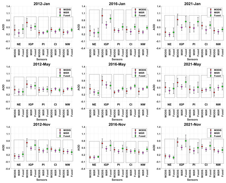
Figure 8 The regional mean values of MODIS, MISR, and fused AOD. On the y axis, AOD values are shown as mean ± standard deviation. Values are provided in Tables S4–S6.

With a view to assessing the improvement in the fused AOD estimates over MODIS and MISR, further analysis is carried out on regional scale considering different sub-regions over the study domain. Figure 8 shows the regional mean values of fused AOD along with AOD from individual satellite sensors. It is observed that the fused AOD significantly improves the biases in AOD from individual sensors. For example, in January 2012, MODIS AOD was significantly higher than fused AOD over IGP, while MISR AOD was closer to fused AOD over NE and CI regions. This indicates that the overestimation by MODIS in the IGP and the underestimation by MISR in the NE and CI regions are effectively corrected by the fusion framework. Similarly, in 2016, MODIS significantly overestimated AOD (∼ 0.99 ± 0.31) in the IGP region. However, this was corrected in the fused AOD ∼ 0.87 ± 0.16, which also closely matches ground-based AOD (∼ 0.86). During the pre-monsoon period, MISR AOD during 2012 and 2016 is closer to fused AOD; whereas in 2021, MODIS is closer to the fused AOD over the NE, IGP, and PI regions than MISR, except over the CI and NW regions. This behavior is consistent with the lower RMSE of MISR relative to ground-based AOD. Post-monsoon analysis reveals MODIS AOD is closer to fused AOD over IGP with an overestimation in 2012 and 2016, and an opposite pattern in 2021. MISR AOD is lower than fused AOD in all these periods. These observations clearly indicate the regional level bias corrections in the individual satellite sensors, resulting in a more accurate representation of aerosol features in terms of fused AOD.

3.3.4 Performance analysis and cross-validation

The accuracy of fusion can be concluded from the cross-validation analysis. This is characterized by LOOCV method.

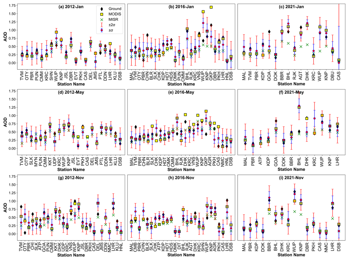
Figure 9 Predicted AOD (magenta points) with error bars ± 1σ (blue line), ± 2σ (red line), along with ground-based (black diamond), MODIS (yellow square), and MISR (green cross) AOD at different stations. For station names refer Table S7 and S8.

Figure 9 shows the predicted AOD values at each ground location during each leave-one-out process. The prediction model performances analyzed in terms of mean prediction error (MPE) and root mean square prediction error (RMSPE) are given in Table 7. The predicted AOD values (as magenta points) at each of the ground locations with standard error bars ± 1σ (blue line), ± 2σ (grey line) are also shown in Fig. 9, along with AOD from the ground (black diamond), MODIS (yellow triangle), MISR (red cross) observations. The figure shows that more than 80 % of ground AOD are within ± 2σ (95 % Confidence interval) of predicted AOD. The highest accuracy was achieved in 2021 November and 2012 May (100 %), and the lowest in 2016 May (76 %), indicating the importance of the association between different sensors during the fusion process. The enhanced accuracy of the model for fused estimations required good correlation and reduced errors, as indicated in Tables 4–7.

Table 7 Accuracy assessment of the predicted AOD through LOOCV. Here % describes how many ground AOD (actual values) are covered within the range of predicted AOD. The values in bold are cross validation results indicating good model performance.

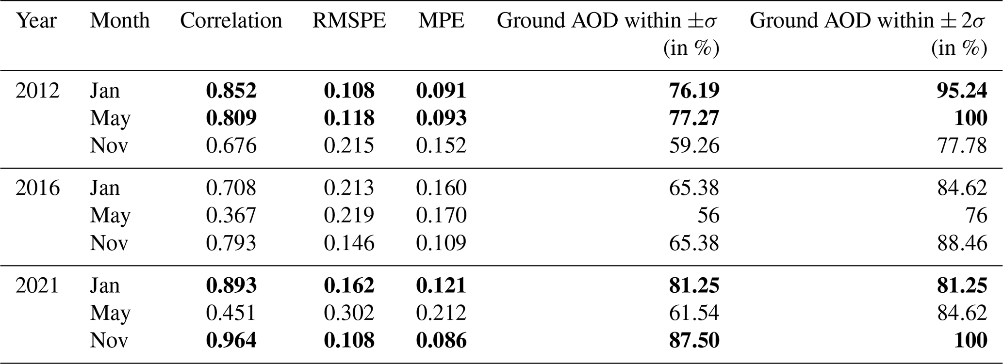
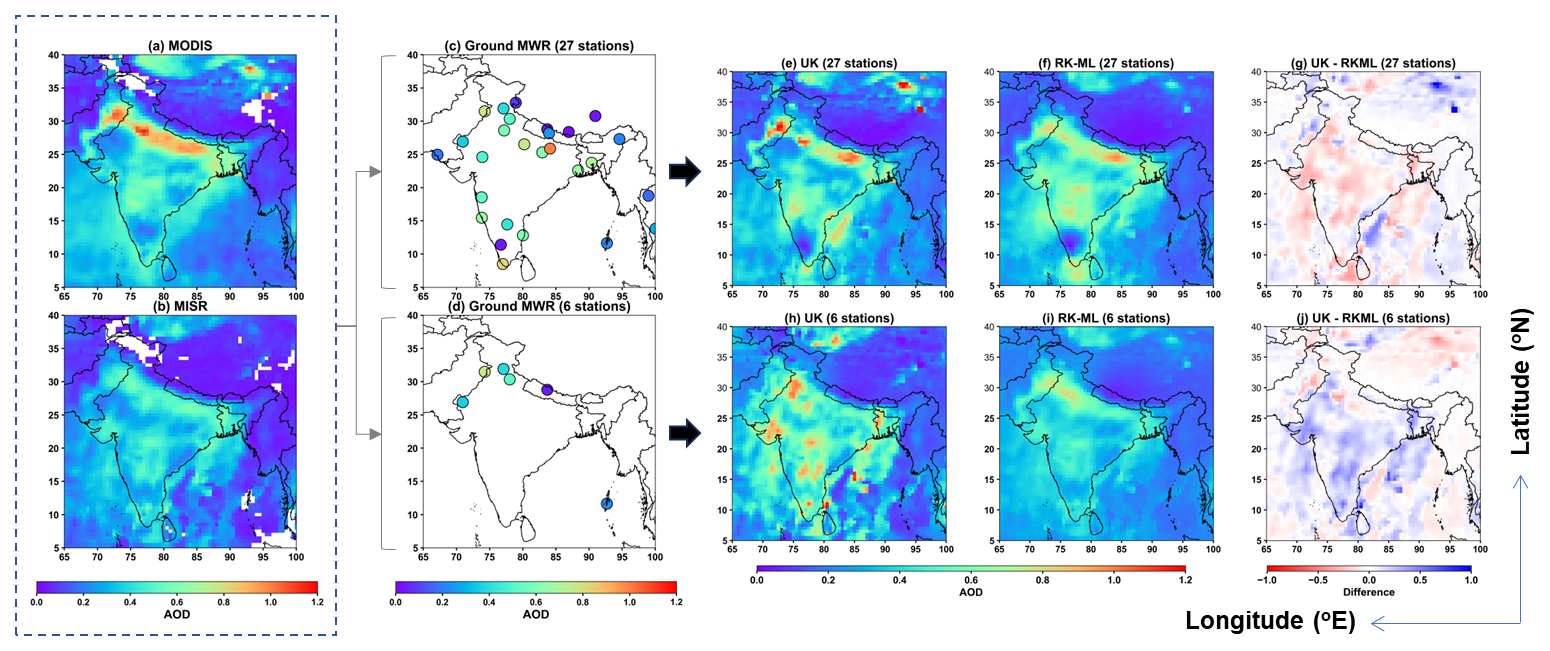
Figure 10 Fused AOD using Universal Kriging (UK, e, h), and Residual Kriging – Machine Learning (RK-ML, f, i) approach for combined MODIS and MISR data sets (a, b) with different number (27 and 6) of ground-location points (c, d). The difference between UK and RK-ML predictions (g, j) are shown, respectively. Blue color in difference map indicates where UK predictions exceed those of RK-ML, and vice versa for red.

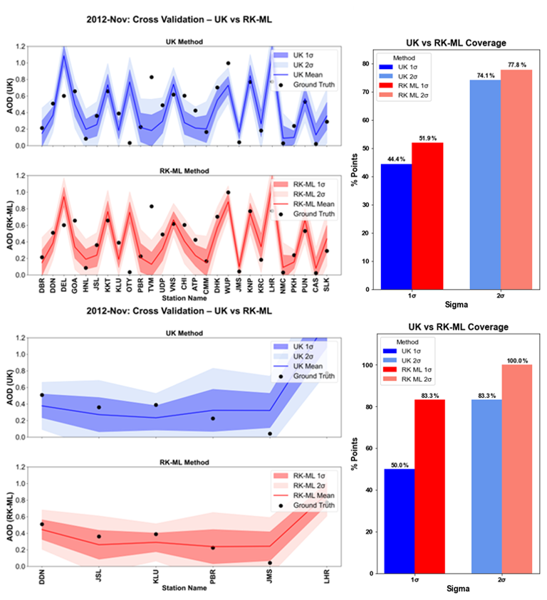
Figure 11 Line plots of LOOCV results from UK method (blue line) and RK-ML method (red line), covering the ground AOD (black dots) for 27 points (top panel line plots) and 6 points (bottom panel line plots) within 1σ (dark shade) and 2σ (light shade). For station names and details, refer to Tables S8 and S9.

3.3.5 Machine Learning enhanced Geostatistical data fusion

To understand the influence of number of ground measurement points in the generation of fused map, sensitivity studies has been carried out by varying the number of ground based measurement points. The number of ground points from maximum of 27 ground locations has been reduced to 22, 13, 8, and 6, respectively. The corresponding variations in the fused outputs are provided in Figs. S36–S38, and Table S9 and a representative case is shown in Fig. 10. The figure clearly explains the changes in prevailing spatial pattern of aerosols according to changes in number of ground points, indicating that both UK and RK-ML methods are suitable for generating fused AOD, when the ground measurements are sufficient (Fig. 10c, e, f, and g). Notably, when data points are fewer, UK overestimates AOD in mainland regions relative to RK-ML predictions (Fig. 10d, h, i, and j). This indicates an inherent limitation in UK method, alike to multiple linear regression models, which are highly susceptible to noise in predictor variables. In contrast, RK-ML demonstrates greater robustness by first modeling the deterministic component using a machine learning regressor (in this case, SVR), followed by Ordinary Kriging (OK) of the residuals to capture the stochastic component. This two-step approach effectively leverages machine learning for optimized estimation under noisy conditions, while OK incorporates spatial variability of residuals obtained from observations, resulting in more reliable spatial predictions. Thus, the advantage of RK-ML for limited ground-points is due to outperformance of OK in comparison to UK, as discussed on basis of different surface types (Zimmerman et al., 1999). Overall, the applicability of UK and RK-ML depends on their ability to capture realistic spatial patterns from spatially representative data points (e.g., ground-based AOD) in order to produce accurate fused AOD distributions. However, as these estimations inherently carry increasing uncertainties with distance from ground observation sites, the resulting maps show elevated uncertainties in areas with sparse ground coverage. As illustrated in Fig. S36, increasing station density enhances the similarity between fusion maps from both methods near the observed ground locations, while locations farther away show greater differences due to differences in mean AOD estimation between the UK and OK methods.

In terms of confidence intervals within ± 1σ and ± 2σ, the performances of UK and RK-ML approach are further evaluated in Fig. 11. The RK-ML predictions are more consistent with the original ground-truth observations within ± 1σ confidence for both sufficient (27) and limited (6) numbers of ground observation points. On the other hand, the performance of UK is consistent with ground-truth observations only when the observations are higher in number.

This is because in UK, the spatial variability is estimated through weights obtained from multiple (sufficient) ground-locations and satellite regressors; hence, trend modeling becomes more robust when a larger number of points are available. These observations clearly suggests that the large number of ground stations are crucial for best representation of fused AOD products from UK, while RK-ML is a good choice in case of limited number of ground observations as it can capture nonlinear relationships and penalize erroneous AOD values.

4 Conclusion

In this study, a data fusion framework for aerosol optical depth (AOD) over India is developed through the evaluation and comparison of two variogram-based geostatistical approaches, namely Universal Kriging (UK) and a novel hybrid residual Kriging–machine learning (RK-ML) method. These approaches differ primarily in the manner in which the mean AOD structure is estimated. Despite inherent differences among instruments, the implemented approach capitalizes on their complementary features, statistically combining two different satellite-based measurements (MODIS and MISR) with ground-based (ARFINET and AERONET) observations, demonstrating enhanced AOD estimation with reduced uncertainties compared to relying on a single instrument. The significant outcomes of this study are as follows:

MODIS and MISR observations exhibit good but variable associations with ground-based AOD measurements influenced by seasonal and geographic differences.

Variogram analysis reveals different autocorrelation length implying capability of each sensor to get the spatial variability or auto correlation structure in different periods. In some of the months, MODIS shows higher spatial range as compared to MISR, while the opposite is seen during the rest of the months. On the other hand, sill is always higher in case of MODIS.

Spatial interpolation of AOD through variogram analysis provides very good predictions at the missing grids of the satellite observations, emphasizing the effectiveness of the universal Kriging method.

The fused AOD maps reveal distinct results, highlighting the significant impact of ground-based AOD on the fusion process. The near-perfect correlation (R ∼ 0.99) between fused and ground-based AOD suggests effective bias correction in MODIS or MISR datasets, which otherwise significantly overestimated or underestimated aerosol measurements across certain parts of the study region. Incorporating a greater number of ground-based measurements enhances the fused results.

Leave-One-Out Cross-Validation (LOOCV) of the UK approach suggests that 95 % confidence interval (± 2σ) of the fused AOD captures up to 100 % of ground observations, indicating effectiveness in capturing regional aerosol variability. On the other hand, RK-ML demonstrates more stable spatial patterns and improved LOOCV performance compared to UK, particularly in regions with limited ground-based coverage. The establishment of additional ground-based stations is recommended to strengthen the representation of air quality, especially in regions with high heterogeneity. This methodology can be implemented to get the fusion maps of finer spatiotemporal resolution.