Estimation of Doppler velocity from incoherent scatter spectra using context-aware transformers

We present a context-aware transformer model for estimating Doppler velocity from incoherent scatter radar (ISR) spectra. The model is based on the standard transformer encoder with adaptations from the Vision Transformer. Trained entirely on theoretical spectra, the AI model generalizes well for Arecibo ISR data and outperforms the traditional fitting methods significantly. To assess performance, we compare the plasma drift velocities estimated by the AI model with those from the conventional least-squares fitting (LSF) technique. The analysis is focused near 110 km altitude, where pronounced vertical velocity and electron density gradients provide an environment that most readily highlights the difference between the two estimation methods. Our results show that the LSF velocity error is 1.5 to 3.5 times that of the AI model using 5 input heights. An inference from the AI model is approximately 100 times faster than the LSF method and requires minimal hardware, making it practical for large-scale or real-time processing. Although the AI method is demonstrated for the Arecibo ISR, it can be potentially applied to other cases where the spectra can be parameterized.

1 Introduction

Measuring the Doppler velocity of a medium using the power spectrum is a common problem in many applications (e.g., Fukao and Hamazu, 2014; Richards, 2014). Incoherent scatter radars (ISR) provide one of the most direct and reliable means of measuring ionospheric parameters, including Doppler velocity (e.g., Zhou et al., 1997; Virtanen et al., 2021). This study focuses on accurately determining the ionosphere velocity from the power spectra of ISR. Accurate Doppler velocity measurements are important for understanding ionosphere dynamics, monitoring geomagnetic activity, and improving space weather forecasts (e.g., Zhang et al., 2005; Chau et al., 2009; Hysell et al., 2022; Zhou et al., 2024a).

Doppler velocity from the power spectrum is traditionally derived using three main approaches: the moment, autocorrelation function (ACF), and the least-squares fitting (LSF) method (e.g., Woodman, 1985; Kudeki et al., 1999; Zhou et al., 1997; Chau and Kudeki, 2006; Li and Zhou, 2024). The moment method calculates the first moment of the Doppler power spectrum, yielding a weighted average velocity. The ACF method computes the ratio of the ACF's imaginary to the real part at different lags. The ACF and moment methods require only the power spectrum to be symmetric, but do not need any other knowledge of the power spectrum. Their easy implementations and computational efficiency make them a popular first choice. Nevertheless, the ACF and moment methods can be sensitive to noise and may not always have the desired accuracy. The least-squares fitting (LSF) method compares the measured power spectrum to theoretical spectra and estimates the Doppler shift and spectral width by typically minimizing the least-squares error. This approach is more accurate but computationally more demanding. However, fitting the Doppler shift along with other ionosphere parameters makes the overall fitting less accurate and more difficult to converge on the optimal solution. One way to alleviate the problem is to do a rough estimate of the other parameters while fitting for Doppler (Li and Zhou, 2024).

Recent advances in machine learning have seen the method used in diverse fields. Unlike traditional fitting methods, machine learning models learn directly from data and may surpass traditional approaches, especially under noisy or complex settings. Transformer architectures, in particular, have shown strong results in a range of tasks due to their ability to extract relevant patterns from sequences using self-attention (Vaswani et al. 2017). Although originally developed for natural language processing, they have been adapted to structured inputs. We demonstrate here that transformers can process ISR spectral data and estimate Doppler velocity more accurately than traditional approaches.

In the following two sections, we first describe the ISR data and then the AI model used for this work. In Sect. 4, we compare the AI results with the traditional LSF method using data taken by the Arecibo ISR data to demonstrate the former's advantages.

2 Experimental and training data

All training and evaluation data are synthetically generated using the standard theoretical incoherent scatter spectrum model (Swartz and Farley, 1979; Kudeki and Milla, 2011). Each sample consists of 5 consecutive altitude bins, spaced 300 m apart, with one incoherent scatter spectrum per altitude bin. The spectrum at each altitude is sampled at 101 points between ±12.2 kHz, with a resolution of 244.3 Hz and normalized to have a maximum value of 1. Representative examples of synthetic incoherent scatter spectra at different noise levels can be found in Aponte et al. (2007) and Li and Zhou (2024). The bandwidth and frequency resolution are selected based on the maximum compatibility with the existing Arecibo Observatory ISR data processing workflow described in Li and Zhou (2024). These hyperparameters can be easily modified to support different coding configurations or facilities.

In a typical Arecibo Coded Long Pulse (CLP) configuration with a 2 µs gate width, the full bandwidth is 500 kHz, corresponding to a Doppler aliasing limit of ±87.2 km s⁻¹. The characteristics of the CLP program and the Arecibo instruments can be found in Sulzer (1986), Isham et al. (2000), and Li and Zhou (2024). Typical line-of-sight ion velocities are below ±100 m s⁻¹, corresponding to a Doppler shift of about 287 Hz. The raw spectrum is computed from CLP data with a native resolution of 2.27 kHz and is interpolated to 244.3 Hz using FFT zero padding. The interpolation was originally introduced for compatibility with the LSF method used in Li and Zhou (2024) and is retained in this work without modification.

Although further interpolating the spectrum to a finer frequency grid may appear to be beneficial, we observe no performance gain once the network is sufficiently trained. The input head consists of a multi-layer perceptron (MLP) (Hornik et al., 1989) that processes the spectrum before it enters the transformer blocks. This learned projection serves as a data-driven alternative to fixed interpolation and is likely able to extract sub-bin Doppler information by learning smooth spectral structures directly from the input. Because the MLP operates across all frequency bins simultaneously, it can learn to resolve fine-grained shifts and spectral shapes without relying on increased frequency resolution.

In the synthesized training data, the Doppler velocity is randomly assigned for each sample, drawn uniformly from −100 to 100 m s⁻¹. The signal-to-noise ratio (SNR) is also randomly assigned, following a logarithmic distribution between 5 and 50 dB, representing the range from low-quality to near noise-free ISR measurements. All other plasma parameters, including electron density (N_e), electron temperature (T_e), ion temperature (T_i), and the ion fractions of H⁺, He⁺, O⁺, and O${}_{\mathrm{2}}^{+}$, are randomly sampled from real ISR measurements obtained through traditional LSF methods as discussed in Li and Zhou (2024, 2025).

We test two types of AI models in this study. The first one treats all the heights independently, which we will call context-unaware models. The second one, referred to as context-aware, assumes the ionospheric parameters within a pre-defined range of heights are interrelated. For the context-aware models, each of the model parameters (including SNR) within the interconnected heights is approximated by the expression

$$\begin{array}{}\text{(1)}& y\left(i\right)=X_{\mathrm{0}}+\left(X_{\mathrm{1}}-X_{\mathrm{0}}\right){\left({\displaystyle \frac{i}{N}}\right)}^{\mathit{\alpha }},i=\mathrm{1},\mathrm{2},\mathrm{\dots },N\end{array}$$

where N is the number of consecutive altitude bins, X₀ and X₁ are the lower and upper bounds of the parameter value, centered around a given input value with a random range of variation up to 10 %. For this study, we chose N = 5 for our context-aware model. The case of N = 1 is the context-unaware model that processes the data at each altitude independently. The exponent α is randomly selected from either the concave down range [1, 1.1], which produces a gently decreasing slope, or the concave up range [0.9, 1.0], which produces a curve that rises more steeply at lower altitudes and flattens at the top. Each curve is flipped in order with 50 % probability to allow both increasing and decreasing trends. Including a synthetic gradient makes the training profiles more realistic, but its impact on performance is limited unless N becomes large. For the relatively small N (= 5) used for the current work, the model is largely information-limited, so the structure introduced in Eq. (1) does not substantially change model performance. At the same time, over-representing extreme or non-representative gradient cases in the synthetic training set can shift the training distribution away from the target data and bias the model toward rare structures, which can degrade performance on typical observations. For this reason, the training set is designed to reflect the empirical distribution of gradients seen in real data. The context-aware model effectively reduces the resolution from 1 to N heights with a weighted average while the running average reduces the resolution by assuming all the N heights have an equal weight.

An offset is used across the N heights to ensure the value at index integer $(N/\mathrm{2})+\mathrm{1}$ equals the originally sampled target value. A total of 2 million training samples are generated using this process. An independent test set of 100 000 samples is constructed using the same procedure. This approach is consistent with broader definitions of physics-informed machine learning, where domain knowledge from ISR theory is used to generate and constrain the training data, rather than being explicitly hard-coded into the network architecture or loss function.

3 Method

3.1 AI architecture

We follow the standard transformer encoder architecture originally introduced by Vaswani et al. (2017), which has become a widely used neural network model for analyzing structured, high-dimensional data. In contrast to traditional convolutional or recurrent neural networks, transformer models are based on a self-attention mechanism that explicitly learns relationships between all elements of the input simultaneously. This allows the model to capture long-range dependencies and global context in the data, rather than relying only on local neighborhood information. As a result, transformers are particularly effective in problems where weak or subtle signals are distributed across the full input domain and cannot be reliably identified by localized features alone.

In recent years, transformer architecture has been successfully adapted beyond natural language processing to scientific and imaging applications. One notable example is the Vision Transformer (ViT) by Dosovitskiy et al. (2020), which reformulates image analysis as a sequence-learning problem. In the ViT approach, an image is decomposed into a set of patches, each treated as an input token, and the transformer encoder learns the global relationships among these patches through attention. A token in this context is one element of the input sequence, represented as a feature vector.

The present work adopts a ViT-style formulation for altitude-resolved ISR ion-line spectra, in which each altitude bin is represented as a token, with the corresponding frequency-resolved spectrum forming the feature vector of the corresponding token. This representation is well suited to the Doppler estimation problem, as Doppler shifts are manifested as altitudinally coherent displacements embedded in spectra whose widths and amplitudes vary with local plasma parameters. By enabling joint attention across all altitude bins, the transformer can leverage contextual information from the full profile to stabilize Doppler estimates in the presence of thermal broadening and noise.

For brevity, we do not reproduce the full mathematical formulation of the transformer encoder and attention mechanism here, and instead refer the reader to Vaswani et al. (2017) for the original architecture and Dosovitskiy et al. (2020) for its ViT adaptation. The specific architectural modifications and training configuration used in this study are described in the following subsections.

The input of the net consists of spectral measurements across multiple altitudes, originally structured as a grid of 101 frequency points by 5 heights. The 5 × 101 input (altitude × frequency) is treated as a sequence of five frequency-resolved spectra. A one-dimensional convolution (Conv1D) layer applies the same learned linear filter to each 101-point spectrum, mapping it to a 512-dimensional feature vector; the kernel size and stride are both 101, so the operation acts independently on each altitude bin. Collecting the resulting feature vectors forms a 5 × 512 tensor, i.e., a two-dimensional numerical array representing five tokens with 512 features each.

As the transformer itself is invariant to the order of input tokens, it does not encode the relative ordering of altitude bins by default. However, altitude ordering is physically meaningful for ISR spectra, as neighboring heights share similar plasma conditions. To provide this information, we add trainable positional encodings to each altitude token. These encodings are learned vectors that act as an altitude-dependent bias added to the token features, allowing the model to distinguish and learn spatial relationships along the vertical dimension. We note that the positional coding is only for the N context-aware heights. Adjacent non-overlapping groups of heights are independent.

With the input tokens augmented by positional information, the resulting sequence is then processed by a stack of transformer encoder blocks. Each transformer block consists of a multi-head self-attention mechanism (Vaswani et al. 2017) followed by a feed-forward network, with residual connections (He et al., 2016) and layer normalization (Ba et al., 2016) applied at each sublayer. We adopt a pre-normalization configuration, where layer normalization is applied before both the attention and feed-forward modules to improve training stability in deeper networks.

A dedicated trainable classification token, commonly referred to as [CLS] token in AI literature (Devlin et al., 2019), is prepended to the input sequence and serves as a summary representation. In transformer architectures such as BERT or ViT (Devlin et al., 2019; Dosovitskiy et al., 2020), the [CLS] token interacts with all tokens via self-attention and is used as the final input to the regression head. We also evaluate an alternative strategy using global average pooling across all token outputs, as discussed in Sect. 3.2. An overview of the model architecture is shown in Fig. 1.

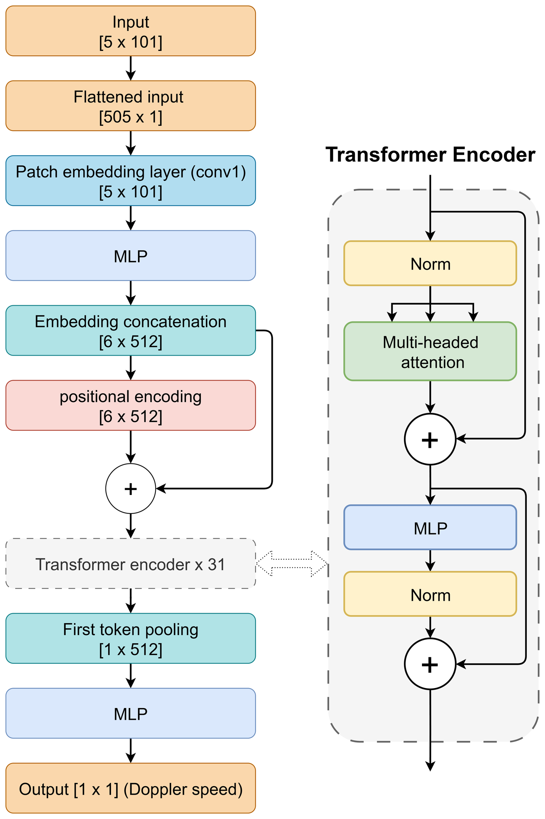
Figure 1 Model overview. The architecture consists of 31 transformer encoder blocks, 321 layers in total, and approximately 100 million parameters.

3.2 Training of the AI model

The model is trained using about 2 million synthetic samples and validated on 10 000 synthetic validation samples. The training uses mini-batches with a batch size of 512. A mini-batch is a small chunk of the training data that was used to do one model update. Larger batches improve computational efficiency but increase memory usage. Smaller batch size uses less memory and sometimes leads to better generalization, at the cost of training speed. In machine learning, generalization means the model's performance on new, unseen data. We train for 30 epochs, where one epoch denotes one full pass through the entire training set. Model parameters are optimized with the Adam optimizer (Kingma and Ba, 2015), an adaptive first-order stochastic optimization method widely used for deep networks, and mean squared error (MSE) as the cost function. We use a cosine learning rate schedule (cosine annealing) with a linear warmup, i.e., the learning rate increases linearly from 10⁻⁷ to 10⁻⁴ during the first 1000 iterations, then decays following a cosine curve back to 10⁻⁷ by the final epoch. Learning rate is the step size the optimizer uses when it updates the model parameters. Cosine schedules (Loshchilov and Hutter, 2016) are commonly used to improve optimization stability and final convergence.

Layer-wise Learning Rate Decay (LLRD, Howard and Ruder, 2018) is a fine-tuning strategy also referred to as discriminative fine-tuning. It assigns smaller learning rates to lower (earlier) layers and larger learning rates to higher (later) layers, reflecting the idea that early layers often learn more general representations while later layers are more task-specific. LLRD is widely used in natural language processing. In our application, we find LLRD is important for stable training, particularly for deeper architectures. Without LLRD, increasing the number of transformer blocks often degrades performance (i.e., deeper models fail to benefit from scaling). While our model can operate with as few as one transformer block, we tested depths up to 100 blocks and observed consistent performance gains across this range. We therefore choose a 31-block architecture as a practical trade-off among hardware compatibility, inference speed, and model performance, and use LLRD with a decay rate of 0.9 per block to stabilize training and support scaling.

3.3 Simulations and comparisons

We evaluate two key design choices in the model architecture: whether to use the full altitude-resolved ISR input or an averaged spectrum, and whether to aggregate token representations using a [CLS] token or global average pooling. The context-aware version (5ht-aware) treats each of the 5 altitude levels as a separate input token, preserving vertical structure and allowing the transformer to model inter-altitude dependencies through self-attention. The context-unaware version (context-unaware) averages the 5 spectra into a single profile, removing altitude information.

For aggregation, we compare global average pooling to a trainable [CLS] token. In the pooling variant, token outputs from the final transformer layer are averaged before being passed to the regression head. In the [CLS] configuration, a trainable token is prepended to the sequence and extracted after the final layer, allowing the model to learn a global representation directly from the full token set.

We first compare the two aggregation methods using the context-aware input. Once the better aggregation strategy is determined, we fix it and evaluate the impact of vertical context by comparing the context-aware and context-unaware variants. Finally, the traditional LSF method is included as a reference for comparison against the best-performing deep learning model.

3.3.1 CLS vs. global pooling

The two aggregation strategies differ in how the final representation is derived and fed to the output MLP. In the [CLS] configuration, a trainable [CLS] token is prepended to the input sequence before positional encoding. After passing through the transformer layers, only the final state of the [CLS] token is used as input to the output MLP, which produces the Doppler velocity prediction. In the global average pooling variant, no [CLS] token is used. Instead, the outputs of all tokens from the final transformer layer are averaged along the sequence dimension, and this pooled vector is passed to the output MLP. Both configurations use the same output head architecture, but differ in how information from the sequence is aggregated.

Our experiments show that the [CLS] aggregation strategy consistently outperforms global average pooling in terms of RMSE and scalability. With a shallow 2-block model, [CLS] achieves about 2 % lower RMSE than global pooling. As the model scales to 31 blocks, the gap widens to roughly 5 %. In contrast, global pooling does not benefit from increased depth, as deeper models show no performance gain and often exhibit unstable training behavior. Although global pooling may occasionally match the [CLS] model on specific validation runs, its overall performance is less stable. These findings indicate that global pooling is less effective in our setting and that the [CLS] token provides more robust and scalable performance.

3.3.2 Context awareness

In traditional ISR spectral fitting, range integration or vertical smoothing is often applied before parameter estimation. This reduces noise by averaging incoherent scatter spectra across altitude, but removes vertical structure. The context-unaware model adopts the same approach by averaging the 5 × 101 input across altitude into a single 101-point spectrum, treated as one altitude. Since self-attention requires multiple tokens, the 101-point spectrum is reshaped into 101 tokens with one feature each so that attention operates along the spectral dimension.

The context-aware model retains the vertical structure by treating each altitude within the aware range as a separate token. It takes all 5 incoherent scatter spectra directly, with each token representing one altitude and containing a 101-point spectrum. The transformer receives all 5 tokens and returns a single Doppler velocity prediction. The middle altitude bin (3rd height) is used as the prediction target.

Both the context-aware and context-unaware models use the same 31-block [CLS]-based architecture and the same underlying data (and noise), but are trained and tested with different input formats. The context-aware model receives the full 5 × 101 height-resolved spectra. The context-unaware model receives the same data after averaging the five heights, i.e., the 5 × 101 input is averaged to 1 × 101 and reshaped to 101 × 1.

To benchmark model performance, we compare the AI models against two LSF baselines using simulated data. The first scenario, LSF-ideal, assumes access to the true (noise-free) spectrum with known amplitude, which is not achievable in real measurements. The second, LSF-realistic, follows the approach discussed in Li and Zhou (2024, 2025), where plasma parameters, including Doppler velocity, are estimated from noisy spectra through parameterized fitting. Both LSF methods use the averaged spectrum from five heights to match the resolution of the AI models.

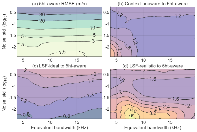
Figure 2 (a) RMSE (m s⁻¹) as a function of noise standard deviation and equivalent bandwidth for 5ht-aware model. RMSE ratio of context-unaware (b), LSF-ideal (c) and LSF-realistic (d) to 5ht-aware model. In the LSF-ideal case, the spectrum shape parameters are given as a priori information. In the LSF-realistic case, the spectral shape parameters are unknown and must be estimated.

Figure 2a shows the root mean squared error (RMSE) as a function of the noise standard deviation (η) and equivalent spectral bandwidth for the 5ht-aware model. Figure 2b–d show the RMSE ratios of the 5ht-aware model to the other three methods. The equivalent bandwidth characterizes the effective spectral width of the incoherent scatter spectrum and reflects the combined influence of ion temperature, mass, and composition (Zhou, 2002). Its range in Fig. 2 spans the 430 MHz incoherent scatter spectral bandwidth from the E-region to the topside. In the simulations, the ground truth Doppler velocities follow a uniform distribution in the range between −85 to 85 m s⁻¹. The velocity RMSE from the 5ht-aware model in Fig. 2a increases with η as expected. When η is above 30 (∼ 10^1.5), the velocity RMSE is largely independent of the equivalent bandwidth.

The context-aware model consistently achieves lower RMSE than the LSF-realistic and context-unaware models across the full practical range of η values and equivalent bandwidths. While arithmetic averaging is most effective in reducing uncorrelated stationary Gaussian noise, the context-aware model implicitly functions as a denoising network. It has prior knowledge of the typical spectral shapes at different heights and learns to extract consistent features across the noisy inputs. As a result, it may suppress noise more effectively than simple arithmetic averaging and hence outperforms the context-unaware model. The LSF-ideal method outperforms the 5ht-aware model in the low noise regime, where the input spectrum is nearly noise-free and the fitting problem is well-conditioned. In this case, the spectrum is effectively a clean copy of the known target, and the algorithm can retrieve the Doppler largely without error, except for a small quantization error due to the finite velocity grid resolution. LSF-ideal and LSF-realistic differ in how the spectrum used for Doppler fitting is obtained. In the LSF-ideal case, the true noise-free spectrum shape is assumed to be known, and the Doppler velocity is retrieved by shifting this fixed template along the frequency axis and minimizing the least-squares error. In the LSF-realistic case, the spectrum shape is unknown and must first be estimated from noisy data. The RMSE of the LSF-realistic method is about 1.5 and 3.5 times that of the 5ht-aware model for η at 0.1 and 0.01, respectively.

In Fig. 3, we compare the performances of the 5ht-aware, LSF-realistic and the moment method as a function of altitude for a representative condition at Arecibo. The altitude-dependent noise variance profile is sampled from an Arecibo Observatory measurement on 11 September 2014, increasing from 10^−4.2 at 90 km to 10⁻³ at 200 km. Here we consider not only the noise standard deviation as in Fig. 2, but also the bias as well. The velocity bias and standard deviation (σ) are obtained from 24,795 runs with the same input velocity and noise standard deviation, η. The velocity is made to change with the altitude as $v\left(z\right)=A\left(z\right)\cos \left(\frac{\mathrm{2}\mathit{\pi }}{{\left(z-\mathrm{60}\right)}^{\mathrm{0.8}}}(z-\mathrm{90})\right)$, where $A\left(z\right)=\mathrm{50}\left(\mathrm{1}-e^{-\frac{z-\mathrm{90}}{\mathrm{10}}}\right)$ and z is the altitude in km. $v\left(z\right)/\mathrm{30}$ is depicted in Fig. 3a as a dotted magenta line. The other three lines in Fig. 3a are the biases, defined as the input velocity minus the results from the three methods. The ionosphere parameters and η are taken from representative daytime measurements on 12 April 2013 at Arecibo. The 5ht-aware model has a comparable bias to the LSF method. The bias of LSF-realistic is approximately 3 % of the true velocity for the noise standard deviation used. In the extreme case of all noise and no signal, the mean LSF and moment velocities tend to zero because the estimated velocities are symmetrically distributed at positive and negative values. Similarly, as long as there is noise, LSF and moment techniques tend to underestimate the velocity amplitude. It is of interest to note that the largest biases of the 5ht-aware model occur at the middle of the velocity range, likely due to the model's effort to compensate for the larger bias typically associated with higher velocities. LSF's standard deviation (σ_LSF) does not only depend on η but also on the velocity amplitude. σ_Moment is linearly proportional to η for all the altitudes. σ_AI is the smallest among the three methods. To quantitatively show the improvement of the AI over the other two methods, we plot the ratio of velocity standard deviations in Fig. 3c. Averaging over 87 to 193 km, σ_AI is about 64 % and 38 % of σ_LSF and σ_Moment, respectively.

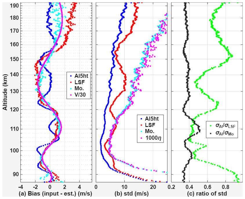
Figure 3 (a) Simulated biases and (b) standard deviations of the AI 5ht-aware model, LSF-realistic, and moment methods as a function of altitude. The magenta curve in panel (b) represents 1000η. (c) Ratios of standard deviation of AI to LSF and moment methods.

4 Application to Arecibo ISR data processing

We apply the analysis technique to the data taken at Arecibo on 16 July 2015. We will mainly focus on the comparison in the E-region around 110 km where the vertical velocity and electron density gradients are larger than in the F-region. The larger gradients limit the height range one can integrate, and the effect of different signal processing techniques can be more readily seen. During the period, the Arecibo linefeed rotated back and forth in the azimuth direction at a slew rate of 24° min⁻¹ with a constant zenith angle of 15°. The raw data were processed to mitigate the interferences as discussed in Zhou et al. (2024b) before computing the spectra. Figure 4a and b show the line-of-sight velocities from the context-aware model and the LSF method discussed above. The integration time for the power spectrum is 30 s. The setup is the same as in the above section, i.e., the power spectra are integrated over 5 heights to have a range resolution of 1.5 km, and the number of aware heights in the AI context-aware model is also 5 to have the same height resolution as the LSF method. As seen in the above section, the context-unaware and moment methods are inferior to the 5ht-aware and LSF-realistic method, respectively, and will not be discussed in this section.

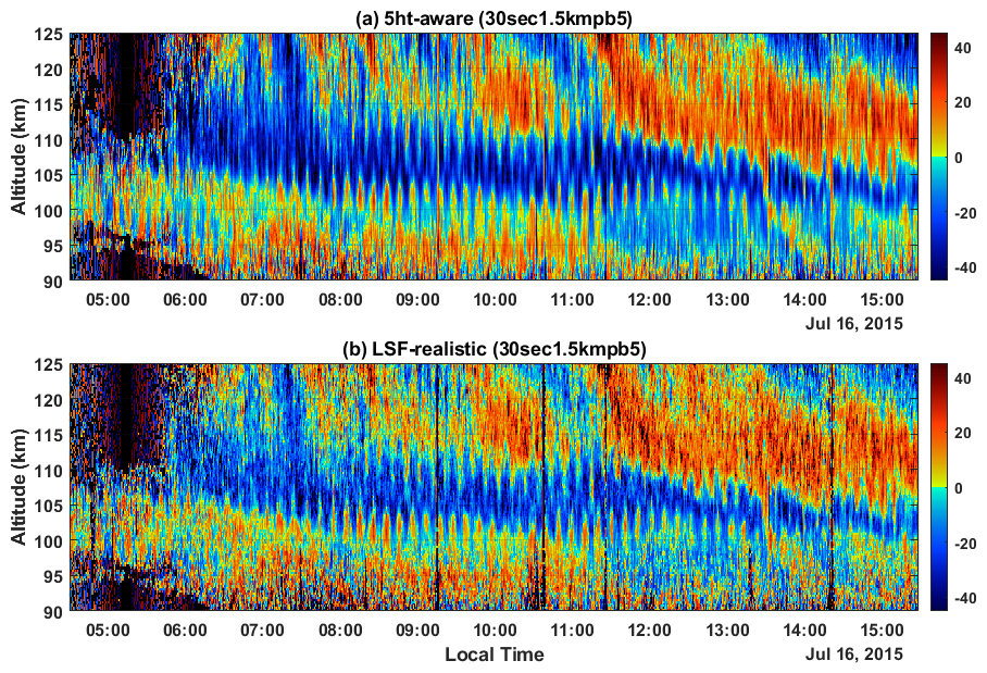
Figure 4 (a) Line-of-sight velocity derived from the 5ht-aware model, (b) from the LSF-realistic method. Positive velocity is away from the radar.

The line-of-sight velocity, V_r, is a superposition of the horizontal and vertical velocities. The vertical stripes in the velocity plots are due to the constant rotation of the antenna. As we do not expect V_r to change randomly, its height coherence reflects the data quality. As seen from Fig. 4, the AI plot shows better coherence than the LSF plot in the bottom. This is more clearly seen between 90 to 100 km and between 120 and 125 km. The amplitude in the LSF plot is smaller, as discussed above.

We use the standard deviation of the second-order difference to estimate the velocity error. The second order difference, y, of a signal, x, at time (or height) t_i is $y\left(t_i\right)=x(t_i+\mathrm{\Delta }{t}_i)-\mathrm{2}x\left(t_i\right)+x(t_i-\mathrm{\Delta }{t}_i)$, where Δt_i is the minimum sampling interval to ensure independence among x(t_i+Δt_i), x(t_i) and x(t_i−Δt_i). For a slowly varying signal with superposed noise, the variance of y is 6 times the variance of x for independent samples, which is the case in our analysis. The standard deviation of the second-order difference of independent samples is thus $\sqrt{\mathrm{6}}$ times of the random error, as measured by the standard deviation. Figure 5a shows statistical errors (divided by 40) of the 5ht-aware model (blue dots) and the LSF method (red dots) when the 2nd order partial difference is taken in the altitude direction. The error profiles are similar to that shown Fig. 3c, and the lowest error occurs at an altitude of 100 km. Both AI and LSF errors increase almost linearly from 100 to about 180 km due to the increase in spectral width, and hardly vary below the F-region peak from 180 to 300 km. The average electron density profile for this period is plotted as a black line for background information. The average F-region peak altitude during this period is at 330 km. The error ratio of the 5ht-aware model to the LSF-realistic method, γ, is plotted as a green line. In Fig. 5a, where the error is based on the 2nd order difference in altitude, γ is largely a constant above 120 km at 0.55. Below 100 km, γ is about 0.4. The ∼ 50 % error reduction in the AI model in Fig. 5a is largely consistent with the results shown in Figs. 3c and 2d.

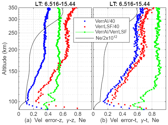
Figure 5 (a) Average velocity errors (divided by 40) estimated from the 2nd order difference in altitude using the AI 5ht-aware model and the LSF-realistic method over the period of 06:30–15:25 LT on 16 July 2015. The green line is the ratio of AI to LSF error. The black line is the average electron density. (b) Same as panel (a) except that the 2nd order difference is taken in the time direction.

We can also estimate the error by taking the 2nd order partial difference with respect to time. The results are shown in Fig. 5b. The AI error is much larger than that in Fig. 5a even though the error trends remain the same while the LSF error is not much affected. A possible explanation for the difference in the error behaviors in Fig. 5a and b is that the noise baseline, which needs to be subtracted from the spectrum before Doppler processing, is a function of frequency as well as time. How the noise baseline is estimated affects the results. It impacts the LSF method less because the fitting error is already large due to statistical fluctuation. Another possibility is that the standard deviation also contains non-linear temporal variations in the velocity field. In any event, the AI error is still 30 % smaller than the LSF method around 110 km, which is the focus of the current study. Above 120 km, a larger number of heights can be used in the context-aware model to reduce the error.

In this study, the AI context-aware model uses 5 heights to allow a good height resolution (1.5 km) for the E-region. At altitude ranges where coarser height resolution is acceptable, the number of heights in the context-aware model can be increased. This further elevates the advantage of the AI method. For example, the error ratio of the LSF-realistic to the AI context-aware model using 9 input heights is larger than 2 in practically all scenarios. Beyond accuracy, the proposed transformer model also offers a clear computational advantage over the least-squares fitting method. Once trained, Doppler velocity inference is approximately 100 times faster than LSF and requires substantially fewer computational resources. The model contains approximately 100 million parameters (≈ 300 MB) and runs efficiently for inference on any modern discrete GPU, making it suitable for large-scale data processing and near–real-time applications. Model training is performed using synthetic data and can be completed in approximately two days on a higher-end GPU (e.g., RTX 3090 or above).

5 Discussion and Conclusion

We successfully developed and validated a context-aware transformer model for estimating Doppler velocity from Incoherent Scatter Radar (ISR) spectra. This deep learning approach adapts the Vision Transformer architecture to process multiple altitude-resolved spectra simultaneously, treating each altitude bin as a unique token. The model was trained exclusively on 2 million synthetically generated ISR spectra, which were created using theoretical simulations, allowing for explicit control over parameters like signal-to-noise ratio and Doppler velocity range. This theory-only training can consider all the practical scenarios and ensures the model's strong generalization capability, which is confirmed with real Arecibo ISR data. The key advantage of the context-aware design is its ability to leverage vertical structure and dependencies across adjacent altitude bins, significantly enhancing noise suppression and stabilizing the Doppler estimates. In addition to accuracy, the transformer offers a substantial computational advantage. Model training requires approximately a one-time cost of one day using an Nvidia RTX5090 graphics processor. Meanwhile, the LSF baseline incurs repeated runtime costs and can require days to weeks to process a few days of radar measurements, whereas the trained model can process the same data in a few hours.

Although our focus is on the Arecibo ISR at 430 MHz, the approach applies to other ISRs and non-ISR situations as long as the spectra can be parameterized. The AI model used here will likely outperform the LSF method in most of the other scenarios as well. In training the AI model for ISR applications, the only radar parameter that comes into play is the transmitting frequency unless the radar is pointed exactly perpendicular to the geomagnetic field line. Other radar parameters affect SNR, which can be adjusted by changing the height and/or time resolution. In any event, we have tested a large range of SNR and spectral widths, covering practically all the situations in which a useful Doppler can be obtained for UHF radars. Incoherent scatter fitting methods are generally known to be easily adaptable to different radars. There is no reason to believe that the advantages of the AI model discussed here do not apply to other ISRs.

Incoherent power spectra shapes are complex and diverse in the altitude range discussed here, including Gaussian-like and superpositions of Gaussian-like functions. If the model works for the ISR spectra, it will likely work for simpler non-ISR spectra as well, since those spectra are similar to subsets of the ISR spectra. Further, in dealing with sharp vertical changes in any of the state variables, such as the electron density in sporadic E's, one can either reduce the number of heights in the awareness model or use a combination of the height-aware model and height-unaware model. Other than needing to train a different model, the AI model does not have any greater limitations than the LSF method in achieving different height resolutions.

In conclusion, we have introduced an accurate, computationally fast, and highly generalizable AI solution for Doppler velocity determination. Simulations and applications to Arecibo Incoherent Scatter Radar measurements consistently show that the proposed context-aware transformer-based AI model achieves lower error than the LSF method for both synthetic test cases and Arecibo observations. As the training data are generated using physics-based ISR simulations, SNR and Doppler velocity range can be explicitly controlled during data generation. Therefore, the proposed framework is not inherently limited to the Arecibo ISR and can be adapted to other instruments by retraining the model using instrument-specific parameters and configurations. In fact, the approach applies to any situation where the observed spectra can be parameterized, and the parameter to be estimated is not limited to Doppler. In a subsequent work, we have demonstrated that AI-based models can outperform LSF in estimating helium and hydrogen ion fractions as well as electron and ion temperatures in the upper F-region (Li and Zhou, 2026). The new paradigm in ISR data processing can enhance the study of ionospheric dynamics and space weather monitoring capability.