Optimizing airborne emission rate retrievals with sub-hectometre resolution numerical modelling

A comprehensive model-based study is designed to provide optimal flight paths for airborne top-down emission rate retrieval methodologies. The meteorology and plume dispersion were modelled using the Weather Research and Forecasting (WRF) modelling platform with the Advanced Research WRF (ARW) dynamical core at 50-m resolution. Multiple flight path designs and parameters were investigated to determine emission rate retrieval accuracy for emissions of a trace gas as a function of downwind distance and transect spacing, which are ultimately related to flight time and cost. Three unique source types (multiple smokestack plumes, small area sources, and a large area source) were investigated for 4 summer afternoon flight cases over 2 d. The results demonstrate that emissions estimate uncertainty is primarily due to storage and release, with uncertainties as high as 30 % at optimal downwind distances (which vary by source type). Interpolation of the sparse measurements can be a significant source of error close to the source, but the uncertainty is ≤17 % for D≥6 km. The average advective flux estimates are within 12 % of the known emissions for downwind distance of D≥4 km. Variability between flights decreases with D. For stack sources the variability near D=10 km is approximately half that at D=4 km. For small area sources, there is less reduction with D, and for the large area source, variability reaches a minimum at D=8 km. For stack sources, vertical spacing of transects is optimized at 100 m, while for area sources, a spacing of 50 m reduces uncertainty. Error due to extrapolation below the lowest flight path is less than 20 % for stack sources and less than 30 % for area sources for non-dimensionalized downwind distance of $D{}^{\prime }\ge \mathrm{3}$. Results demonstrate the need for surface sampling coincident with the flights to reduce extrapolation error, and the use of modeling with reanalysis data to account for storage and release effects.

1 Introduction

During airborne field studies for top-down retrieval of source emission rates, the environmental fields (meteorology and pollutant concentrations) are sampled around and/or downwind of emission sources. Typically, the aircraft flies in a repeating pattern that either encloses the source area (e.g., Peischl et al., 2010; Kalthoff et al., 2002; Gordon et al., 2015; Kim et al., 2025), or that captures the extent of a downwind plume (e.g. Cambaliza et al., 2014). The temporal and spatial resolutions of such measurements are determined by the sampling frequency and range of the measuring instruments, the speed of the sampling platform, the sampling path and geographical locations (Gordon et al., 2015; Conley et al., 2017). The sparse spatial measurements that are made over time are processed and analyzed according to various assumptions regarding how representative they are of the mean and real-time environmental conditions (e.g., wind field, emissions: Alfieri et al., 2010). The post-processed data are then used for estimating emission rates from sources of pollution (Ryoo et al., 2019; Karion et al., 2013; Gordon et al., 2015).

Regardless of the measurement approach, the spatial heterogeneity and temporal variability of meteorology and concentration fields can result in large uncertainties in top-down estimates. Previous studies have attributed large uncertainties (20 % to 40 %) to the gap of information (spatial and temporal) in the sampled data (e.g., Angevine et al., 2020). For instance, airborne measurements are commonly made at elevations above 150 m agl for safety considerations. Gordon et al. (2015) identified the unsampled region below the lowest flight level as a large source of uncertainty in mass-balance analysis (e.g., up to 26 % for CH₄ plumes). The gap of information in the sampled data, due to limitations on spatio-temporal resolution and range of the sampling method, can be partially filled by combining data from different measurement platforms. For instance, airborne samplings (aircraft, UAV) can be complimented by ground-based measurements (Brus et al., 2021b; Bell et al., 2021; Islam et al., 2021). Fixed location in-situ measurement techniques of meteorology and tracer concentrations include tower measurements at heights of up to 350 m a.g.l. (Heintzenberg et al., 2011; Andreae et al., 2015), and radiosonde (tethered/balloon) measurements include heights up to 2 km a.g.l. (Nygård et al., 2017; Nambiar et al., 2020). Ground-based remote-sensing can also be conducted from mobile surface land vehicles (de Boer et al., 2021; Davis et al., 2019), generating column measurements at higher spatial (horizontal) resolution. Remote-sensing datasets can be analyzed in conjunction with airborne measurements for both validation (Davis et al., 2020) and as complementary information (Krings et al., 2018; Brus et al., 2021a) in air quality studies. In a study based on the same model output used in this study, Fathi (2022) suggests augmenting airborne in-situ measurements with aircraft-based remote sensing (lidar) towards improving aircraft mass-balance retrievals.

Dispersion models have also been used to infer emissions from aircraft measurements, as alternative to the more common mass-balance approach. For example, Karion et al. (2019) used an inverse approach comparing different dispersion models (HYSPLIT, STILT, LPDM, FLEXPART) that optimizes emission rates to best fit observation. However, there was significant range in the predicted emission rate depending on the model used. Simpler, Gaussian footprint models can also be used to similar effect (Kim et al., 2025). These techniques offer the advantage of being able to estimate emission rates from multiple sources when the plumes overlap (e.g. Kostinek et al., 2021; Ražnjević et al., 2022). Estimating separate emission rates for each source is more difficult to do with the mass-balance method and requires individual plumes to be well defined and separate (e.g. Baray et al., 2018).

To better understand the mass-balance method and to quantify uncertainties, models can also be used to optimize the mass-balance measurement technique. Virtual aircraft can fly through model output fields, where emissions are known and the relative contributions of advection, turbulence, and flux below the lowest flight path can be determined. This also allows different flight configurations to be compared and optimized to increase emission measurement accuracy as a function of flight time (cost). Panitz et al. (2002) were the first (to our knowledge) to use model output to evaluate the aircraft mass-balance method. They used the KAMM/DRAIS model system to evaluate box flight measurements described in Kalthoff et al. (2002). They determined advective fluxes were 85 % of NO emissions and 95 % of CO emissions, suggesting that total emissions estimated based on downwind advective flux measurements, could be underestimated by up to 15 % (for NO) or 5 % (for CO) by neglecting other terms in the mass-balance equation. Both Tadić et al. (2017) and Conley et al. (2017) appear to be the first to fly a spiral (or cylinder) flight pattern, which was proposed in Gordon et al. (2015) and also used in Han et al. (2024). Conley et al. (2017) ran LES simulations to optimize the spiral radius and the number of passes. It is demonstrated that a minimum non-dimensional radius can be determined, as

$$\begin{array}{}\text{(1)}& R{}^{\prime }={\displaystyle \frac{R{w}_{\ast }}{U{z}_i}}\end{array}$$

where R is the actual radius, w_∗ convective velocity, U mean wind speed, and z_i boundary-layer height. A value of $R{}^{\prime }>\mathrm{0.45}$ resulted in nearly constant concentration below the lowest flight path (150 m), which reduces the uncertainty due to extrapolation of these unknown values. Using order-of-magnitude estimates of $w_{\ast }=\mathrm{1}$ m s⁻¹, z_i=1000 m, and U=10 m s⁻¹, gives R=4.5 km (as an example). Conley et al. (2017) also test the number of laps around the source required to reach convergence over multiple tests and find that 15 or more laps (at a normalized radius of $R^{\prime }=\mathrm{0.25}$) are required to repeatedly produce the most accurate results (which is an accuracy of near 85 % in this case). However, a real-life controlled release experiment suggests that as many as 25 laps are required to reach comparable accuracy.

This study aims to optimize flights to determine emission rates from large emitting stacks in industrial complexes such as the Canadian oil sands (Liggio et al., 2019; Li et al., 2017). These kinds of operations typically include stack emissions, dust and vehicle exhaust from roadways that connect different operations, surface sources of pollution that span over a large area such as surface mine excavation sites, and larger area sources such as tailings ponds (Baray et al., 2018; Davis et al., 2020).

Various emission scenarios (e.g., point, area sources) and tracer dispersion and transport under different meteorological conditions were simulated using a high-resolution WRF model described in Fathi et al. (2023). The output data from this high-resolution (with LES parameterization) WRF model is assessed here as a proxy for real-world environmental fields (virtual sampling). The range of spatial and temporal variability in fields sampled by a mobile platform for top-down retrievals can impact the accuracy of the estimates. For example, spatio-temporal variability in sampled fields is dependent on the downwind distance and hence investigating the optimized sampling distance using model data (following Conley et al., 2017) is desirable and can provide valuable advice in terms of observational flight planning and data processing. By studying the output fields from several different WRF simulation scenarios, we investigate the impact of different sampling strategies on the accuracy of top-down estimates and provide operational recommendations for general and specific cases.

2 Methods

2.1 Case Studies and Location

This analysis uses WRF output data described in Fathi et al. (2023). The WRF model output data span a geographical location over the northwest portion of Athabasca oil sands region, Alberta, Canada. Although three different cases were simulated in Fathi et al. (2023), we focus here on Case 1 on 20 August (all dates in 2013) and Case 3 on 2 September. Case 2 on 26 August was a stagnant, low-wind speed case with high vertical wind shear. For this case, the vertical motion of the plume in the presence of strong wind shear resulted in plume recirculation causing significant storage within the control volume during the flight time. Hence. Case 2 was not considered suitable for the mass-balance technique (see also Fathi et al., 2021 for more discussion of this effect). The dates of Case 1 and 3 coincide with aircraft emission retrieval flights over the CNRL facility in the northwest area of the oil sands region, during the 2013 JOSM (Joint Canada-Alberta Implementation Plan on Oil Sands Monitoring) field campaign (JOSM, 2013) and they are the two flights described in detail in Gordon et al. (2015). Both cases (summer, afternoon flight times) demonstrate thermally and dynamically unstable conditions in both the measurements (Gordon et al., 2015) and model output (Fathi et al., 2023).

2.2 Model Description

Model details are discussed in Fathi et al. (2023) and are summarized here. The Weather Research and Forecasting model (WRF, version 3.9) was used with the ARW dynamical core. In this analysis, we use the velocity components (u, v, w), meteorological parameters (temperature, pressure, and water vapour mixing ratio), and 11 tracer scalars, corresponding to different point, line, and area emission sources (described below). ARW solves for advection of momentum, scalars, and geopotential in flux form (the governing equations).

Five nested grid domains are used in both the horizontal and vertical, with increasing horizontal resolution from 31.25 km to 50 m, and vertical resolution of 11.62 m (for the lowest 40 grid levels in the finest domain), and a time step of 0.16 s (in the finest domain). This resolution is often referred to as “super-resolution” (Wu et al., 2021; Onishi et al., 2019; and Watson et al., 2020). The coarsest domain was driven with North American Regional Reanalysis (NARR) GRIB (GRIdded Binary) data (at 3 h intervals, 31.25 km resolution) from NOAA (National Oceanic and Atmospheric Administration) archives. Our WRF-ARW model configuration conserves mass within 1 %–5 % and successfully resolves turbulent eddies at aircraft-observed scales by leveraging the full suite of large-eddy simulation (LES) options. For details of the super-resolution modelling setup, see Fathi et al. (2023).

We use 7 modeled emission locations in this analysis, which are described in Fathi et al. (2023). The locations are shown in Fig. 1. These are comprised of 4 elevated (stack) sources, two small area surface sources (surface mines), and a large area source (tailings pond). The stacks (CNRL1-4) have respective heights of 114, 54, 30, and 54 m. The large area source (POND) is approximately 50 km², and the small area sources (MINE1 and MINE2) are 550 m × 550 m and 350 m × 550 m, respectively. Each source in the model emits a known amount, E_S, which can be compared to the emissions determined from the TERRA mass-balance method, E_Total, discussed in Sect. 2.3. Emissions from each source are independent in the model and are treated separately. Each of the 4 stacks emits at the same rate and the area sources all emit at the same rate per unit area. Here we group the different emission source types together: stacks (the sum of CNRL1, 2, 3, and 4), small area sources (the sum of MINE1 and MINE2), and the large area source (POND), and we investigate each of the three groups separately. Emissions are all treated as trace gas. These results could be extrapolated to particulate emissions (which would be expected from an area source such as an open pit mine); however, dust processes such as gravitational settling and deposition are not considered here.

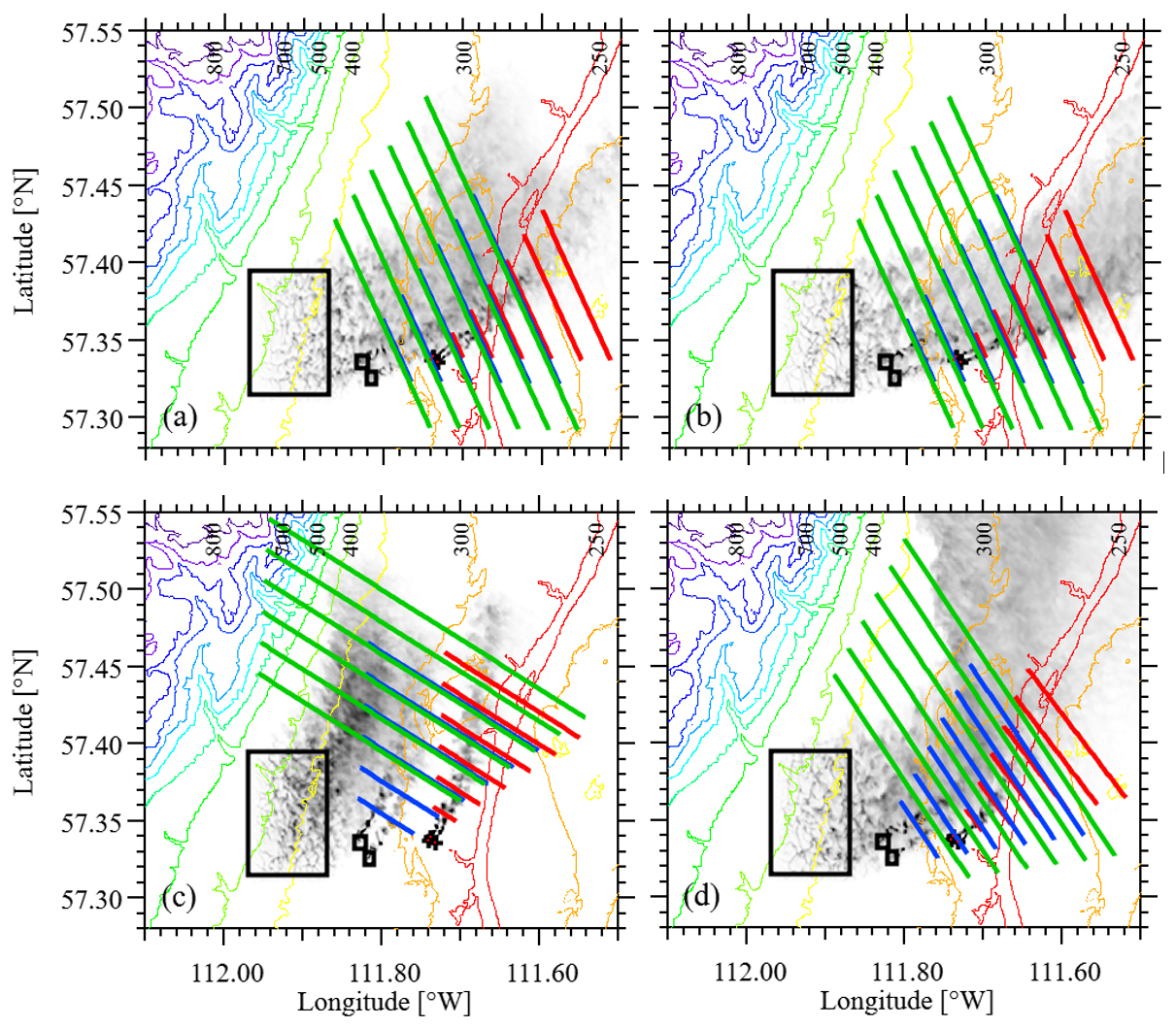
Figure 1 Topography (meters above sea-level) of the finest model domain showing source locations for the stacks (plus symbols), two small area sources, and the large area source (black rectangles). Emissions from all stacks are followed using a single tracer in the model. Emissions from two small area sources are grouped similarly. Plumes (integrated total concentrations with arbitrary scales) are shown as instantaneous snapshots at 20 August 16:20 (a) and 17:20 (b), and 2 September 16:20 (c) and 17:10 (d). Flight paths are shown for each of the three source locations at downwind distances of D=2, 4, 6, 8, 10, and 12 km for the stack sources (red lines), the small area sources (blue lines), and the large area source (green lines). The model domain extends to 57.15° N, but only north of 57.28° N is shown here.

Meteorological and tracer values were output from the finest domain every 1-s over the area shown in Fig. 1 (also extending south of what is shown in the figure to 57.15 °N). Model runs start at 09:00 local time (15:00 UTC). The 20 August run stops at 18:47 UTC and the 2 September run stops at 18:09 UTC. As discussed in Fathi et al. (2023), meteorological fields converge in under 1 h of simulation. All analysis discussed herein starts after 16:20 UTC (80 min after startup) to allow sufficient model spin-up time for the meteorological fields to converge over the modelling domain and ensure that all the plumes have reached the edge of the model domain.

2.3 Mass-Balance Calculation

Airborne top-down emission rate retrievals are usually accomplished by flying at a distance downwind of the emission source and at several altitude levels. Although flights that are far enough downwind of a source (or over a large homogenous surface source) can assume a well mixed boundary layer and fly at a single altitude (e.g. Turnbull et al., 2011; Karion et al., 2013; Hiller et al., 2014), we restrict our analysis here to relatively short flights (∼10's of km) where the plume is not uniformly mixed and flights at multiple heights are required to characterize the plume (Fig. 1).

Following the TERRA algorithm outlined in Gordon et al. (2015) the emission rate within a control volume can be calculated as

$$\begin{array}{}\text{(2)}& E_{\mathrm{Total}}=E_{\mathrm{H}}+E_{\mathrm{HT}}+E_{\mathrm{V}}+E_{\mathrm{VT}}+E_{\mathrm{VD}}-E_{\mathrm{M}}-E_X+S\end{array}$$

where E_Total is the total emissions rate integrated over all activities within the facility, E_H is the horizontal advective flux through the box walls, E_HT is the horizontal turbulent flux through the box walls, E_V is the advective flux through the box top, E_VT is the turbulent flux through the box top, E_VD is the deposition to the surface, E_M is the increase in mass within the volume due to a change in air density, and E_X is the increase in mass due to chemical changes of the compound within the box volume. As demonstrated in Fathi et al. (2021), a storage term (S) must be included to account for emissions trapped within the control volume or released from the control volume after a previous build-up. Fathi et al. (2021) demonstrate that storage/release is related to non-steady state wind conditions, changes in stability, vertical wind shear, and upwind emissions (for enclosed flight patterns). A significant part of the storage term can be due to eddies and circulation at scales comparable to the control volume or flight time. As horizontal winds decrease (or increase), the total concentration within the volume will increase giving S>0 (or decrease giving S<0). Very generally, the horizontal turbulence term (E_HT) estimates flux due to boundary-layer turbulence, while the storage term (S) estimates flux due to mesoscale turbulence. However, as discussed in Fathi et al. (2021), storage can also include the effects of any non-steady-state conditions. For example, changes in atmospheric stability can modify the plume's buoyancy, moving the plume to different heights and resulting in changes in the horizontal advection speed of the plume.

As past studies have shown (Kalthoff et al., 2002; Gordon et al., 2015), the most significant term in Eq. (2) is the horizontal advective flux. This is calculated by first creating a 2-D screen from the flight measurements (using some form of interpolation), with horizontal dimension s, and vertical dimension z, transformed from the 4-D ($x,y,z,t$) measurements The advective flux is then calculated as

$$\begin{array}{}\text{(3)}& E_{\mathrm{H}}=\int \int C{U}_{\perp }\mathrm{d}s\mathrm{d}z\end{array}$$

where s is the distance along the flight path, z is the height from the ground, C is the species concentration at each screen location (s,z), and U_⊥ is the wind speed perpendicular to the screen at each screen location (s,z), calculated as $U_{\perp }=\mathit{U}\cdot \widehat{n}$, where $\widehat{n}$ is the unit vector (horizontal) normal to the flight path, s (positive outward). Both C and U_⊥ are typically measured simultaneously (or close to it) during the flight, which accounts for variation in the wind pattern across the area of the screen.

The simplest and lowest cost approach (i.e. least flight time) is to ignore the control volume and fly in a single screen downwind of the plume (e.g. Mays et al., 2009; Cambaliza et al., 2014). A background concentration must be calculated either from an upwind pass or from the plume edges. The terms E_V, E_VT, and E_M in Eq. (2) can be assumed negligible (provided there is no indication of the plume reaching higher flight levels, and no deep convection is observed). The terms E_HT, E_VD, and E_X can be estimated if the plume source location is known. When multiple downwind screens are used, this method can be used to estimate deposition (E_VD) in the area between the screens (e.g. Liggio et al., 2019; Hayden et al., 2021).

To assess the upwind fluxes and to better estimate all the terms in Eq. (2), the plane can fly in a repeating closed circuit at different heights to trace a 3-D prism or a cylinder. In actual flights at this location (Gordon et al., 2015; Liggio et al., 2019; He et al., 2024), rectangular “box” shapes (or a 5-sided near-rectangle with a cut corner) were flown with sides aligned with compass directions (and facility roads and layouts). In this study, we focus only on screen flights and then extrapolate these results to estimate the uncertainties in enclosed flight patterns. To calculate the emission rate for an enclosed cylinder or box flight, the perpendicular wind speed (U_⊥) in Eq. (2) must take into account the changing flight path direction.

The data (wind and concentration) along the flight path ($x,y,z,t$) within the model are sampled from the model values at the nearest grid location. No interpolation is done within the grid-cell or time-step. The sampling locations are then mapped to screen locations (s,z), and interpolation of the 2D screens is done with the kriging method, which is standard for multiple-path screen flights (e.g. Cambaliza et al., 2014; Gordon et al., 2015; Ryoo et al., 2019; Kim et al., 2025). The kriging algorithm used here (Wavemetrics) fits a spherical function to the variogram to determine the appropriate range value. We also compare results using an exponential variogram model and a Voronoi nearest-neighbour interpolation. In all cases, the screens are interpolated to a resolution of 40 m × 20 m (s and z respectively).

Although various extrapolation methods are available to fill the values between the lowest flight path and the ground (Gordon et al., 2015), for simplicity we assume a constant value between the ground and lower flight path equal to the concentration at the height of the lowest flight path. As discussed above, Conley et al. (2017) determine the optimized flight radius (R^′ in Eq. 1) for a cylindrical pattern as the minimum downwind distance at which the concentration is uniformly mixed (constant) below the lower flight path. Here, we use known model output to optimize the flight distance based on downwind distance of the screen and we investigate the accuracy of this extrapolation method, and whether other extrapolation methods (e.g. linear to zero at the surface, half-Gaussian) would improve emission estimation.

The second largest term in Eq. (2) is typically the storage term, although it is never (to the authors' knowledge) accounted for in mass-balance estimation. Conley et al. (2017) include the flux divergence (analogous to storage/release) in their derivation but demonstrate that it is at least an order of magnitude less than the gradient term (as estimated by the advective flux) under ideal conditions. Reproducing actually flown box-flight patterns (as part of the JOSM campaign) on the same days simulated in this study (20 August and 2 September), and sampling SO₂ (primarily from stack sources), Fathi et al. (2021) found that the ratio of the storage term to the known emission rate ($S/E_{\mathrm{S}}$) was −3 % for the 20 August flights and −29 % for the 2 September flights (negative storage is termed release and represents net loss from the control volume enclosed by the box flight after a previous build-up). Using the same model setup discussed in this paper, Fathi et al. (2023) determined the storage term for a box flight enclosing all the sources with an east wall 5 km downwind of the stack locations. The ratio of the storage term to the known emission rate ($S/E_{\mathrm{S}}$) for the emissions released from the 4 existing stacks (CNRL1-4), the surface mines (MINE), and the tailings pond (POND), ranged from −10.9 % to −2.9 % for 20 August and −27.5 % to 15.4 % for 2 September. Hence, storage can be significant even when winds appear to be steady state, and optimization of flight parameters must consider how to reduce this uncertainty.

2.4 Flight Design

2.4.1 Flight Parameters

Screen and circuit emission retrieval flights can be flown with a variety of aircraft sizes, including UAVs (Han et al., 2024; Yong et al., 2024), small aircraft such as Cesna (Krings et al. 2018; Fiehn et al., 2020; Conley et al., 2017), or larger aircraft, such as Convair (Gordon et al., 2015; Liggio et al., 2019; Kim et al., 2025). UAV speeds range from 2 to 18 m s⁻¹, small aircraft typically fly between 40 and 75 m s⁻¹, while larger aircraft flight near 100 m s⁻¹ and up to 150 m s⁻¹. Sampling rates can vary from 0.5 to as high as 10 Hz (e.g. France et al., 2021), depending on the instrument used, resulting in a wide variety of horizontal sampling scales. In this study, we use a sample distance of 100 m (100 m s⁻¹ at 1 Hz) to fly through the model space, following the scale of actual studies done at this location (e.g. Gordon et al., 2015; Liggio et al., 2019). These results can potentially be scaled to smaller aircraft sizes (or UAVs).

The lowest flight path is taken as 150 m a.g.l. (above ground level), following standard restrictions (e.g. Gordon et al., 2015; Conley et al., 2017). We assume an upward flight path, starting at 150 m a.g.l. and moving upward to a new height after each circuit or screen transect. During an actual field campaign, the concentrations can be monitored in real time, and sampling can be stopped after the last transect samples only background concentration (to avoid wasted flight time). To mimic this in model space, the aircraft flies through the model up to a height of 800 m (well above all tracer emissions), but upper transects above the first background-level transect are removed from the analysis and not counted towards the total flight time.

Multiple screens are flown at distances D=2, 4, 6, 8, 10, and 12 km downwind of the smokestack location or edge of the line or area source. To account for plume spread, the screen length is determined as $L=L_{\mathrm{0}}+\mathrm{2}D\sin \mathit{\phi }$, where L₀ is the width of the line or area source perpendicular to the wind (L₀=0 for smokestack sources), and φ accounts for the spread of the plume with downwind distance. Based on visual inspection of the plume spread in the model, we choose φ=30° to ensure the entire plume is captured under varying wind conditions. For smokestacks, this simplifies to L=D. Figure 1 shows the resulting screen lengths. In actual flights, the screen length may be determined in real time by observing concentrations while flying through the plume, although in some cases a predetermined flight configuration may be required.

For these screens, an initial value of the vertical transect spacing (i.e. the height between each subsequent pass along the screen length) is set to ΔZ=100 m, to match the horizontal spacing. Once the screen distance is optimized, the transect vertical spacing is optimized for that distance by analyzing flights with T values of 50, 100, 150, and 200 m. At the end of each transect, 1 min is added to turn the aircraft around and elevate to the next transect level (based on flight paths from Gordon et al., 2015 and Liggio et al., 2016) but no measurements are taken during these maneuvers.

For each value of D or T, a set of 10 flights are flown to provide a statistical evaluation of the variability and uncertainty in the emissions estimates. For each set of 10 flights, each subsequent flight starts 1 minute later than the start of the previous flight. This offset is added to investigate the uncertainty in the estimated emission rate due to turbulent fluctuations with time scale on the order of 1 to 10 min.

Each flight begins at the most NW location at a height of 150 m a.g.l. There are two sets of flights on each of the two days for each of the three sources. The first set starts at 16:20 UTC. The second set starts at 17:20 UTC on 20 August and 17:10 UTC on 2 September. As explained above, for each set of 10 flights, each subsequent flight within the set starts 1 min later than the previous flight (e.g. start times = 16:20, 16:21... 16:29). To simulate turbulent fluctuations in the flight, at each 1-s timestep of the flight, the horizontal aircraft speed is randomly offset by a Gaussian random number with a standard deviation of 3 m s⁻¹ and the vertical position is offset by a Gaussian random number with a standard deviation of 1 m. These random offsets, although potentially exaggerated compared to the variability of real flight speed or position, were found to produce visually similar flight paths compared to paths shown in Gordon et al. (2015). Given that this is a very subjective comparison, we investigate the effect of reduced offsets in the Supplement (Sect. S2). Although the analysis demonstrates that the effect of the randomized offset is small (<7 % change in the average horizontal advective flux), the temporal and spatial offsets ensures that each of the 10 flights (for each D and ΔZ value) is distinct but generally sampling the same meteorological and emission conditions.

2.4.2 Uncertainty Estimation

Through the statistical analysis of multiple flights, we can also assess how effective repeated flights (or multiple sampling with 2 or 3 UAVs or aircraft) are in reducing the measurement uncertainty in the emission rate estimate. Since subsequent flights may not be statistically independent, we determine the autocorrelation function of the times series of the horizontal advective flux (E_H) for each set of 10 flights. This is used to calculate the effective number of flights, n_eff, following Zięba (2010), which is <10 if subsequent flights are not statistically independent. This gives the effective degrees of freedom for the calculation of the mean (n_eff−1), which can be used to calculate the expanded uncertainty of the mean, following JCGM (2008). If we can assume that the variability within a flight set (σ) is representative of the real variability a flight would encounter under similar conditions, then we can use that value to estimate the uncertainty in a single flight estimate of E_H in the real world. Using the value of n_eff=7 as an example, we are 95 % certain that a single estimate is within 2.45σ of the actual mean E_H value (Table G2 in JCGM for 6° of freedom and a 95 % confidence interval). If, for example, two real flights can be flown (far enough apart in time to assume they are independent measurements), then this uncertainty in the estimate of E_H is reduced by √2 to 1.41σ. It is noted that the uncertainty calculated here effectively combines our uncertainty in the variability in the flights due to a limited number of samples (approximately 26 %, since an infinite number of flights would reduce 2.45σ to 1.95σ) with the actual variability between flights, which could be due to storage fluctuations, interpolation/extrapolation errors, or sparse sampling.

2.4.3 Instantaneous Screens

For comparison, we also output the full model screen at one instant in time. In this case, the concentration at all grid cells along the screen (between the surface and 800 m a.g.l.) is output. This calculates all the tracer mass passing through the screen at a given time, removing the effect of spatially sampling a temporally changing environment. By sampling at the grid square spacing from the surface (i.e. no lowest flight path height restriction), this removes the uncertainty associated with both kriging interpolation and extrapolation below the lowest flight path. These screens are sampled (at the grid square spacing) at downwind distances of D=2, 6, and 10 km. To investigate the variability of the E_H value estimated by this method (primarily associated with the storage term, S), 10 flights are flown at each distance, starting at 16:20 UTC with each subsequent screen 1 min later. We refer to these calculated emission rates as “instantaneous”.

The instantaneous screens are also used to test and compare the image interpolation methods. In these cases, we use the flight path positions described above (s,z) and sample the concentrations at those positions from the instantaneous screens. Each series of points sampled from an instantaneous screen is then used to create an interpolated screen, which can be directly compared to the instantaneous screen at the same resolution. This allows us to isolate the error caused by image interpolation alone. We can also calculate the error associated with the extrapolation of a constant concentration below the lowest flight path.

2.5 Meteorological Conditions

Figure 2 show the temperature (T) and winds (U,V) from the model at a height of 150 m above ground level for the two dates at three locations: the stacks, the centre of the small area sources, and the centre of the large area source. The flight durations are also shown for comparison (straight lines on the T-axis) for the two sets of flights on each date. The instantaneous flights (the shortest lines) span 9 min (e.g. 16:20, 16:21... 16:29). The longest screens downwind of the stack sources (at D=12 km) span approximately 27 min, including 18 min of flight time plus 9 min since each of the 10 flights is offset by 1 min each. Similarly, the longest small area and large area flight sets span 32 and 49 min, respectively. Screen flights closer to the source are always shorter in duration since the screen lengths are shorter, the plume tends to be lower to the ground and less transects are required to capture the entire plume.

The friction velocity (u_∗) and the bulk Richardson number (Ri) demonstrate the turbulence and the stability conditions, respectively. The largest bulk Richardson number (shown in Fig. 2 as a negative value on a log scale) is $Ri=-\mathrm{0.49}$, which demonstrates that the conditions are always turbulent and likely unstable during these model runs. Temperature rises consistently during both afternoons, by approximately 3 °C on 20 August and 4 °C on 2 September. Although these two afternoons were chosen for their steady-state conditions, the winds can vary considerably over time and between different locations, demonstrating potential for storage and release during the flights.

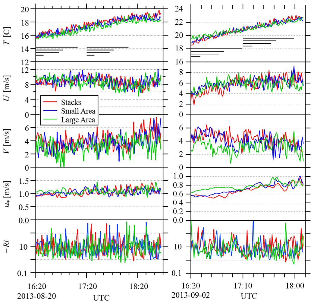
Figure 2 Meteorological variables during the model runs at 3 locations: (red) stacks, (blue) centre of small area sources, (green) centre of large area source. Temperature (T) and winds (U,V) are at a height of 150 m. Friction velocity (u_∗) and negative bulk Richardson number (−Ri) are shown. The bulk Richardson number is based on a 10 to 150-m height difference. The straight lines on the T axis show flight durations. From shortest to longest lines, they are: 10 instantaneous flights (spanning 9 min), stack flights, small area flights, and large area flights.

2.6 Enclosed Flights

Although the single-screen flight is the most efficient way to sample emissions since it captures the greatest downwind area without expending flight time flying upwind of the emission source, there are sometimes situations where an enclosed flight path (such as a cylinder or box flight) is necessary. For a small downwind distance, it could be more economical to continue in a circle (or spiral) pattern around the source, eliminating the need for the tight turning circle at the end of each screen transect. Or the aircraft could be equipped to measure multiple pollutants (potentially from multiple sources), and a single, large, enclosed flight path can capture a volume containing all the emission sources better than a single screen much further downwind. Or there may be upwind sources of the pollutant (or a strong background value) that must be subtracted from the horizontal advective flux.

For the stack (i.e. point) sources, calculating the screen length based on an assumed ±30° lateral plume spread results in a screen length that is approximately $\mathrm{1}/\mathrm{6}$ of a total circle circumference. The difference in distance from the source between a circle arc (radius R) and a straight line over a ±30° range is less than 7 % of R. Hence the only significant differences between a spiral or cylinder flight and the downwind screens investigated here would be the extra time required to complete the remaining $\mathrm{5}/\mathrm{6}$ of the circle for each transect (assuming no upwind sources or background concentration). For the stack emissions, we can investigate the difference in emissions estimates by using the same screen configuration, but we add a time offset after each transect to account for the time required to complete the flight path around the source.

We compare the difference between the screen flights and a circular enclosed flight pattern for a downwind distance of D=10 km for the stack sources only. For the stack sources, the screen length at D=10 km is L=10 km. Thus, each screen transect (at a speed of 100 m s⁻¹) takes 100 s. For the circular enclosed flight comparison, we recalculate the flight, adding a 500 s offset to each transect to account for the time required to complete the loop. The flight time required (for all 10 circular enclosed flights) is 91 min in total (16:20 to 17:51 UTC), effectively spanning most of the model output duration and overlapping with both the 16:20 and 17:20 or 17:10 flight sets (Fig. 2).

2.7 Storage Variability

As discussed in Sect. 2.3, Fathi et al. (2021) estimated the ratio of the storage term to the known emission rate ($S/E_{\mathrm{S}}$) based on actual flight paths and Fathi et al. (2023) estimated $S/E_{\mathrm{S}}$ for a modeled flight path for different source emissions. Since the storage term is highly variable and the effect of large-scale turbulent fluctuations can change during the time it takes to fly a screen, we investigate the variability of the storage term for various flight lengths associated with the different flight configurations. The total integrated concentration within each control volume is calculated as a time series for the model run duration on each date. For each flight configuration (3 sources, 6 downwind distances), the control volume is defined as an area enclosed by the screen on the north-east side, extending south to a latitude 2 km south of the source and west to a longitude 2 km west of source, where the 2 km buffer accounts for any upwind diffusion from the source. The time-averaged storage is then determined as the average rate of change in integrated concentration within the volume over that period, which is positive for build up of emissions within the volume or negative for release of material from the volume. The period length investigated corresponds to the average flight time for a given source at a given distance. For example, the average flight lengths for the screen 6 km downwind of the small area sources (on 2 August, 16:20) is 700 s (i.e. approximately 7 transects of 9 km (1.5-min each) plus turning time). The average storage (over 700 s) is then calculated (within the volume enclosing the small area source up to the screen at 6 km) for each 700 s period in the entire 147 min time series (16:20 to 18:47), and the standard deviation of these values (σ_S) is determined. While this cannot give us the exact value of the storage term for each flight investigated (since the plume is sampled at different points in time and space while the storage term is changing), this does provide a quantification of the relative uncertainty due to changing storage for different flight configurations on different dates. The resulting storage variability is discussed in Sect. 3.3.

2.8 Scaling

Although Conley et al. (2017) normalize R (to give R^′ in Eq. 1), in this study we present D as dimensional (km) lengths. To compare both approaches, we non-dimensionalize the downwind distance following Eq. (1) (with D^′ and D instead of R^′ and R) and investigate whether this improves the results in Sect. 3.4. As with Conley et al. (2017), we approximate the convective flux as $w_{\ast }={\mathit{\sigma }}_U/\mathrm{0.6}$, where σ_U is the standard deviation of the horizontal wind speed. The boundary-layer heights (z_i) are output from the model at the source locations. An average value of z_i is determined for each flight set and the effect of boundary-layer growth is discussed below. Using these values with the average wind speeds for each flight duration, D^′ is calculated for each set of 10 flights and we investigate whether this collapses the results for all cases.

3 Results and Discussion

3.1 Stack Sources

3.1.1 Optimizing Screen Flights for D

Figure 3 shows the calculated horizontal advection fluxes (E_H, Eq. 2) for screens at given downwind distances (D) for the 4 cases: 20 August at 16:20 and 17:20, and 2 September at 16:20 and 17:10. The fluxes are calculated for the emissions from the 4 stacks (CNRL1-4) and are normalized by these known emissions (E_S). Each calculated advection flux ($E_{\mathrm{H}}/E_{\mathrm{S}}$) is the average of 10 flights. The standard deviation of $E_{\mathrm{H}}/E_{\mathrm{S}}$ from the 10 flights is shown as both error bars on the average values and absolute values (to clearly demonstrate how σ changes with D). For clarity, in the discussion below all values of $E_{\mathrm{H}}/E_{\mathrm{S}}$ are given as a ratio (e.g. 1.0), while all values of the standard deviation are given as percentages (e.g. 10 %).

At a downwind distance of 2 km the instantaneous screen captures nearly all the stack emissions, with $E_{\mathrm{H}}/E_{\mathrm{S}}$ values ranging from 0.90 and 0.98. This ratio generally increases with downwind distance, except for the 2 September 17:10 flights. Deviation from a ratio of $E_{\mathrm{H}}/E_{\mathrm{S}}=\mathrm{1}$ may be due to uncertainty in the estimated mean (which ranges from 0.24 to 0.35 for these results at a 95 % CI), or one (or more) of the 7 other terms on the right side of Eq. (2) may be non-negligible. As demonstrated in Fathi et al. (2023) there is negative mass creation in the model near the plume emission point (where concentration gradients are large) as an artifact of diffusion and mass conservation schemes common for numerical chemical transport models near sharp gradients in concentration. This is generally consistent with the slight underestimation near the source and the increase in $E_{\mathrm{H}}/E_{\mathrm{S}}$ with downwind distance (for 3 of the 4 cases).

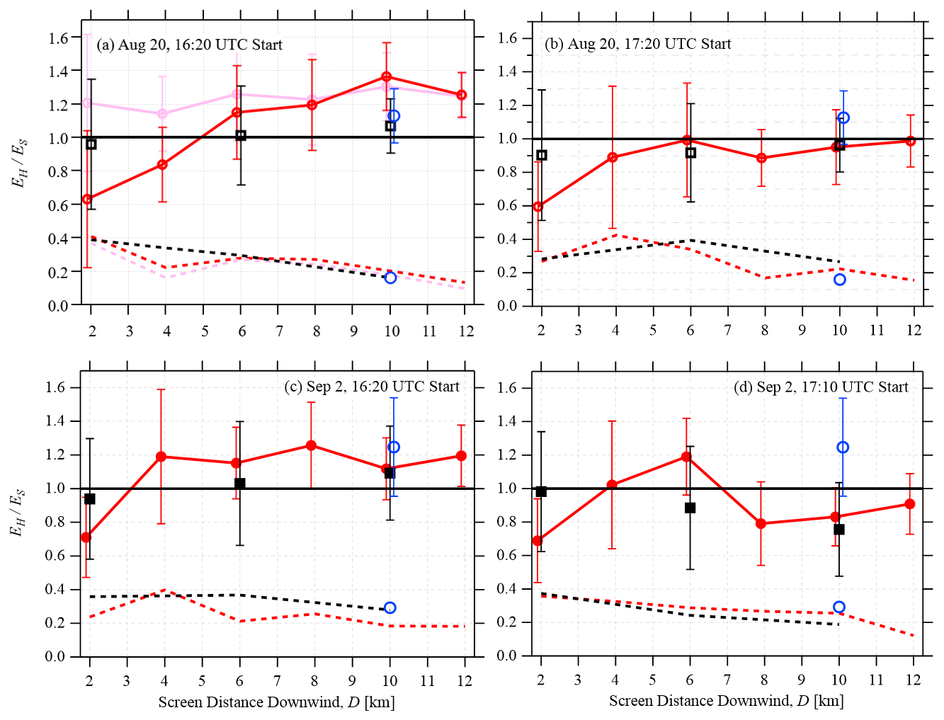
Figure 3 The variation in the ratio of horizontal advection flux (E_H) to the known emission rate (E_S) with downwind screen distance (D) for the stack sources for 4 flight cases: 20 August, starting 16:20 (a) and 17:20 (b), and 2 September, starting 16:20 (c) and 17:10 (d). The black squares are the $E_{\mathrm{H}}/E_{\mathrm{S}}$ values from the instantaneous flight sets. The red circles are the flights through the model (assuming a constant value between the lowest flight path at 150-m and the surface). Error bars show one standard deviation (σ) calculated from 10 flights (offset horizontally for clarity). The dashed lines show σ as absolute values to highlight the change in σ with D. The blue circles are the same variables ($E_{\mathrm{H}}/E_{\mathrm{S}}$ and σ) for 2 enclosed cylindrical flight patterns (on 20 August and 2 September) starting at 16:20 and ending at 17:51. The pink lines in (a) demonstrate a case with additional measurements from a ground-based vehicle, discussed in Supplement (Sect. S1).

At a downwind distance of 2 km, there is substantial variation between the instantaneous flights (σ ranges from 28 % to 41 %). Further from the source, σ generally decreases with D, with values ranging from 19 % to 28 % at a downwind distance of 10 km. From Eq. (2), there may be some variation in horizontal turbulent flux (E_HT) for different flights. Fathi et al. (2023) estimated E_HT as <0.4 % and <1.8 % of E_S for 20 August and 2 September respectively. Since the screen captures the full vertical extent of the plume, E_V and E_VT (flux through the box top) should be zero. There is no deposition or chemistry in the model, so E_VD and E_X are zero. E_M (the change in mass within the volume due to density change) is zero, since the screen is an instantaneous snapshot. Hence, this substantial variation between flights is likely due to storage, with changes in wind speed and direction temporarily changing the advection flux through the screen (i.e. accumulation or subsequent release of pollutant between the stack and the screen). The storage terms estimated for 8 flights in Fathi et al. (2021), excluding a rejected flight, varied from −27 % to 20 %, which is comparable in scale to the variation seen between instantaneous cases here. Storage uncertainty is investigated further in Sect. 3.3.

For the non-instantaneous flights, which include uncertainty due to kriging interpolation and the extrapolation below the lowest flight path height in addition to the uncertainty of storage, the emission rate near the source (at D=2 km) is underestimated by the horizontal advective flux in all cases (ranging from 0.60 to 0.71). Further from the source, at D=6 km, the emissions are either nearly correct (0.99) or overestimated (up to 1.19). Beyond D≥8 km, the estimations vary considerably for different cases (ranging from 0.79 and 1.37). Much of this underestimation and overestimation is likely due to the extrapolation to the surface below the lowest flight path. Figure 4a–d show the profiles of the instantaneous flights, averaged for all 10 flights across the entire flight length. At D=2 km, the plume concentration below 150 m increases with concentration towards the surface, which results in an underestimation of the emission rate (i.e. a lower $E_{\mathrm{H}}/E_{\mathrm{S}}$ value is estimated by the assumed below 150-m concentration relative to what would be determined with the actual below 150-m concentrations). At D=6 km, there is some decrease in concentration towards the surface in 3 of the 4 cases, which results in an overestimation of E_S for that flight. At D=10 km, the concentration is nearly constant with height for the 2 September flights, although there is still substantial variability for the 20 August flights.

The standard deviation of $E_{\mathrm{H}}/E_{\mathrm{S}}$ generally decreases with downwind distance, from as high as 41 % at D=2 km to 12 % at D=12 km. The standard deviations of the instantaneous, known flights for the same downwind distances is similar in magnitude to the variability in the flown sampled flights, suggesting that no substantial variability is added due to either the extrapolation below the lowest flight path, the kriging interpolation of the sparse sampling, or the sampling over an extended period of time (as opposed to an instantaneous snapshot). The decrease in variability with downwind distance suggests that uncertainty in individual flight estimations can be reduced with greater downwind distance, likely due to increased mixing and dispersion with downwind distance and the resulting smoothing of the plume across a larger area. In a real-world scenario, there may be additional error due to variability in the concentration (either due to measurement noise or variability in the concentration due to turbulence), particularly for concentrations with a high background level. In these cases, moving further downwind (where the concentration enhancements above background due to the plume are much smaller), may result in a relative increase in error.

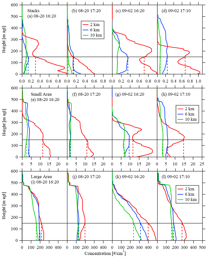
Figure 4 The concentration profiles from the instantaneous screens for the 4 flight cases and 3 source types at various downwind distances. These profiles are ensemble averages of 10 flight profiles averaged across the flight length (L) at each height. The dashed lines compare constant concentration below the lowest flight path (at z_l=150 m).

The non-instantaneous emission estimates may also be higher than the instantaneous emission estimates due to oversampling of a vertically moving plume. If the plume is moving in the same direction as the sampling (upwards in these cases), then the aircraft can sample the same plume multiple times. Conversely an opposite moving plume (downward for upward sampling) will result in under-estimation relative to the instantaneous estimates. This is investigated in Sect. 3.1.3 below. This effect should be reduced with downwind distance as the plume becomes more vertically mixed and spread across a larger height range.

The results demonstrate that it is difficult to determine an optimal flight distance, since there are multiple criteria that include optimization of $E_{\mathrm{H}}/E_{\mathrm{S}}$, reduction of σ, or correct extrapolation below the lowest flight path, and it will depend on the goals of the investigation. The results will also depend on different meteorological conditions (boundary-layer height, variability of winds), as evidenced by the differences between flight cases. Generally, flying too close to the source (D=2 km) results in an underestimation of the emission rate. For D≥4 km, the variation between flights decreases with distance, reaching approximately half its value at 10 km (relative to the value at D=4 km). Flying at a downwind distance of D=10 km, generally results in a constant concentration below the lowest flight path, but the results are still inconsistent at this distance. At a distance of D=10 km, the emission rate at D=10 km varies from 0.83 to 1.37, and the uncertainty in the estimate from a single flight (based on the variability between flights) is as high as 60 % (2.36σ, corresponding to the value of n_eff=8 for these cases, JCGM, 2008).

3.1.2 Optimizing Screen Interpolation

As shown in Fig. 3, the estimation of E_S is generally higher in the non-instantaneous flight sets, relative to the instantaneous flight sets, for D≥6 km, but lower in the non-instantaneous flight sets for D=2 km. This may be due to the kriging interpolation causing an overestimation of the screen concentrations. To test the interpolation, we sampled the instantaneous screens using the non-instantaneous flight path positions, allowing us to compare the interpolated screens with the high-resolution model output screens. We applied the same extrapolation of a constant concentration for heights below 150 m. The average concentration is then calculated from the interpolated screens, $<C_{\mathrm{K}}>$, which can be compared with the average concentration for the model output screens, $<C_{\mathrm{M}}>$. The ratio of $<C_{\mathrm{K}}>$ to $<C_{\mathrm{M}}>$ is shown in Fig. 5, separated into the averages above 150 m and below 150 m (where the concentration is assumed constant). For simplicity, we only compare 2 cases: 20 August and 2 September with 16:20 flight start times.

The differences between the different interpolation methods are small relative to the errors in the interpolation at different downwind distance, D. For z>150 m, kriging with the spherical variogram model gives a slightly better average ($<C_{\mathrm{K}}>/<C_{\mathrm{M}}\mathit{>=}\mathrm{1.07}$ for all downwind distances on 20 August and $<C_{\mathrm{K}}>/<C_{\mathrm{M}}\mathit{>=}\mathrm{1.01}$ for 2 September, versus 1.08 and 1.01 respectively for an exponential variogram model, and 1.10 and 1.03 respectively for the Voronoi nearest neighbour). For the spherical model, the results are also not sensitive to the goodness of fit of the variogram model. For examples, for the 20 August values for z>150 m, halving or doubling the range value of the variogram model changes the average value of $<C_{\mathrm{K}}>/<C_{\mathrm{M}}>$ by less than 2 %. Hence, the choice of interpolation method and the details associated with those choices seems to be less consequential than the changes in the sparseness of the sampling at different downwind distances.

The interpolation for z>150 m generally overestimates the actual concentration and shows high variability between flights when close to the source (D=2 km). Further downwind (D≥6 km), the interpolation is significantly improved and the variability between flights is reduced, with values of $<C_{\mathrm{K}}>/<C_{\mathrm{M}}\mathit{>=}\mathrm{1.00}$ and σ=6 % for the 20 August 16:20 flights, and $<C_{\mathrm{K}}>/<C_{\mathrm{M}}\mathit{>=}\mathrm{1.01}$ and σ=3 % for the 2 September 16:20 flights (both at D=10 km with the spherical kriging).

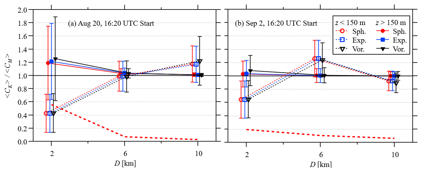
Figure 5 A comparison of average concentration from the instantaneous screens (at downwind distance, D) $<C_{\mathrm{M}}>$, to the average concentration from an interpolation of those flights with sparse sampling $<C_{\mathrm{K}}>$ downwind of stack sources (given as ratio $<C_{\mathrm{K}}>/<C_{\mathrm{M}}>$). The averages are separated into below and above 150 m (open symbols with dotted lines, and closed symbols with solid lines, respectively), where the below 150 m concentrations are assumed constant (see Fig. 4). Three interpolation methods are compared: kriging with a spherical variogram model (red circles), kriging with an exponential variogram model (blue squares), and Voronoi nearest-neighbour (black triangles). The markers are offset slightly for clarity. The standard deviations of the 10 flights (σ) are shown as error bars, as well as red dashed lines for the spherical kriging (>150 m) only. Results are shown for the 20 August (a) and 2 September (b) 16:20 flight sets, corresponding to Fig. 3a and c, respectively.

The total interpolation errors appear correlated with the difference between the instantaneous and non-instantaneous flight set emissions estimates shown in Fig. 3a and c. For example, in Fig. 3a, for the 20 August 16:20 flight set at D=2 km, $E_{\mathrm{H}}/E_{\mathrm{S}}=\mathrm{0.63}$ for interpolated, non-instantaneous flight set, compared to $E_{\mathrm{H}}/E_{\mathrm{S}}=\mathrm{0.96}$ for the instantaneous flight set. Figure 5 for the same flight set (at D=2 km) shows an underestimation with $<C_{\mathrm{K}}>/<C_{\mathrm{M}}\mathit{>=}\mathrm{0.43}$ for z<150 m and $<C_{\mathrm{K}}>/<C_{\mathrm{M}}\mathit{>=}\mathrm{1.19}$ for z>150 m, suggesting a net underestimation (although the relationship between concentration and advection flux is also influenced by wind speed and the total plume concentration above 150 m may not be equal to the total plume concentration below 150 m). Similarly, for most other distances shown in Fig. 5, an underestimation (or overestimation) in $<C_{\mathrm{K}}>/<C_{\mathrm{M}}>$ is generally associated with a similar scale underestimation (or overestimation) in $E_{\mathrm{H}}/E_{\mathrm{S}}$ for the non-instantaneous flight sets relative to the instantaneous flight sets (which are not interpolated). This implies that the sparseness of sampling is a significant source of error for interpolation close to the stack sources (D=2 km), while further downwind (D≥6 km), there can be significant errors due to the extrapolation of a constant concentration below 150 m (as discussed in Sect. 3.1.1 and shown in Fig. 4).

3.1.3 Optimizing Screen Flights for ΔZ

To further optimize the emission estimation as a function of flight time, we test the sensitivity of $E_{\mathrm{H}}/E_{\mathrm{S}}$ to the vertical spacing of the transects at a downwind distance of D=10 km. We compare 2 cases: 20 August and 2 September with 16:20 flight start times. As shown above (Sect. 3.1.2), the errors associated with interpolation (above 150 m) at a distance of D=10 km are small and it may be possible to increase spacing between flight paths without significantly increasing the error. Figure 6 demonstrates the variation in $E_{\mathrm{H}}/E_{\mathrm{S}}$ with transect spacing. For the 20 August flights, emissions are overestimated by a factor between 1.27 and 1.32 with no dependence on ΔZ. For the 2 September flights, the emissions estimate ratio decreases with transect spacing from 1.15 at ΔZ=50 m to 0.94 at ΔZ=200 m. The variability shows no strong pattern with ΔZ and is lowest at a 150-m spacing (18 %) for the 20 August flights, and at a 100-m spacing (15 %) for the 2 September flights. For the 20 August flights, there is little dependence on ΔZ for either $E_{\mathrm{H}}/E_{\mathrm{S}}$ and σ, suggesting that spacing could optimally be increased to 150 or 200 m to reduce flight time; however for the 2 September flights, the ratio $E_{\mathrm{H}}/E_{\mathrm{S}}$ changes significantly with increased spacing, suggesting that spacing of ΔZ>100 m will modify the emissions estimation and result in underprediction.

The transition from overestimation at small spacing to underestimation at larger spacing could be due to vertical movement of the plume opposite to the sampling direction, resulting in transects missing the plume centre at larger spacing. To investigate this, we repeat the flight sets using the same flight paths with the directions reversed (i.e. top-to-bottom). In these cases, the flight begins at 16:20 (for the first flight in the sets) at the highest point and each flight samples at identical locations in the opposite direction, finishing at the lowest point at a height of 150 m. The reversed direction results in significant improvement in the estimation of $E_{\mathrm{H}}/E_{\mathrm{S}}$ for the 20 August flight sets (especially at smaller transect spacing), but increased error for the 2 September flight sets. In both cases, the variability between flights in each set is reduced for a transect spacing of ΔZ=50 m, but is slightly higher than the variability of the bottom-to-top flight sets with ΔZ≥100 m. As mentioned in Sect. 2.4, real flights are often flown in an upward direction so that the vertical extent of the plume can be determined while flying. While it is difficult to know the vertical extent of the plume beforehand (which would be required for a flight in the downward direction), these results demonstrate the potential advantage of flying once in the upward direction, followed by a subequent flight back in the downward direction.

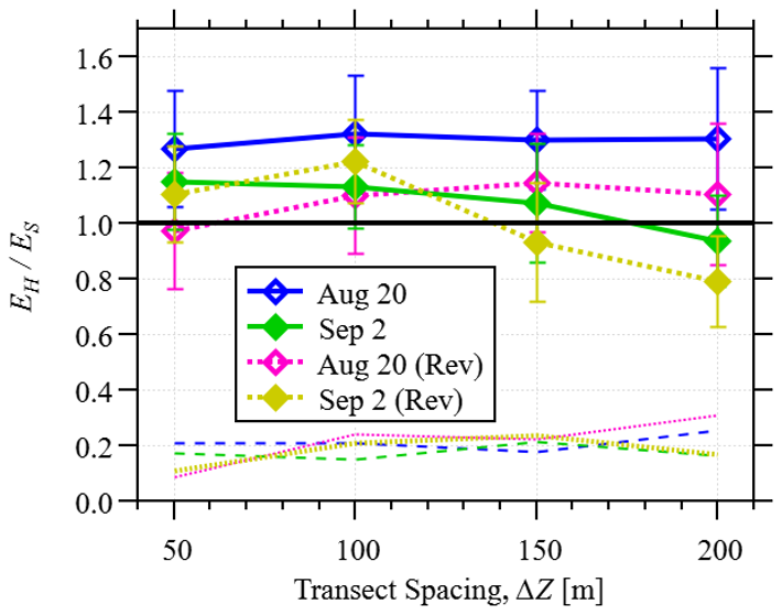
Figure 6 The variation in horizontal advection flux (E_H) to the known emission rate (E_S) with transect spacing (ΔZ) for both the 20 August (blue, open symbols) and 2 September (green, closed symbols) stack source cases with 16:20 flight set start times. Error bars and dashed lines show one standard deviation (calculated from the set of 10 flights). The flight sets are repeated along the same flight paths with a reversed direction (i.e. starting at the top and ending at a height of 150 m) for 20 August (magenta, open symbols, dotted lines) and 2 September (yellow, closed symbols, dotted lines).

3.1.4 Comparing Enclosed Circular Flights

The results form the screen flights show that different conditions at different times of day can lead to error in the emissions estimation, most likely due to storage and release. As discussed above, sometimes enclosed flight designs are necessary. The enclosed flight designs extend the flight time due to the time required to complete the circuit. For our investigated cases here, 2 circular enclosed flights span the flight times of the two screen flight times on each day. On 20 August, the 16:20 screen flight at D=10 km (Fig. 3a) overestimates the emissions (1.37), while the 17:20 screen flight (Fig. 3b) underestimates the emissions (0.95). The circular enclosed flight (Figs. 3a and b) is in the middle of these values (1.13), as might be expected since the sampling is spread out over a longer time. However, this is not the case for the 2 September flights. On 2 September, the 16:20 screen flight at D=10 km (Fig. 3c) similarly overestimates the emissions (1.12), while the 17:10 screen flight (Fig. 3d) underestimates the emissions (0.83), but the circular enclosed flight (Fig. 3c and d) overestimates the emissions (1.26) more than the 16:20 screen flight. For both days, the variability (16% and 29 %) is not substantially different from the variability of the screen flights. Hence, based on this analysis, we cannot conclude that the longer sampling time of the enclosed circular flights modifies the sampling efficiency in any predictable way.

3.2 Area Sources

3.2.1 Optimizing Screen Flights for D

The analysis described above was repeated for the small area (mines) and large area (tailings pond) sources. These sources emit uniformly from the surface within the areas shown in Fig. 1. The resulting horizontal advective fluxes (normalized by the known emission rates) are shown for the small area sources in Fig. 7a–d and for the large area source in Fig. 8a–d. The instantaneous results are inconsistent for the different sources and flights, suggesting that storage may affect the advective fluxes significantly. For the small area sources (Fig. 7a–d), the instantaneous flight horizontal advective fluxes underestimate (or slightly overestimate) the emission rate close (D=2 km) to the source, ranging from 0.74 to 1.01. Beyond this distance, $E_{\mathrm{H}}/E_{\mathrm{S}}$ ranges from 0.87 to 1.15. The non-instantaneous flights closely estimate the emissions in most cases, except for the 2 September 16:20 case, where the emissions are overestimated. For the large area sources on 20 August (Fig. 8a–b), the emissions estimates are generally consistent, ranging from 0.91 to 1.18 (for both instantaneous and non-instantaneous flights). The 2 September flights (Fig. 8c–d) show a strong dependence on D, with both instantaneous and non-instantaneous flights showing similar values. Opposite patterns are seen for the 2 September 16:20 flights (Fig. 8c), emissions are overestimated near the source for D<10 km and underestimated for D≥10 km. For the 2 September 17:10 flights (Fig. 8d), emissions are nearly 1.0 near the source for D≤4 km, underestimated for $\mathrm{6}\le D\le \mathrm{10}$ km and overestimated at D=12 km. This implies that high variability in winds in these cases is leading to storage and release, resulting in build-up and subsequent release of pollutants at different distances downwind of the source. The relatively good agreement between instantaneous and non-instantaneous estimates implies that vertical motion of the plume does not result in over- or under-sampling.

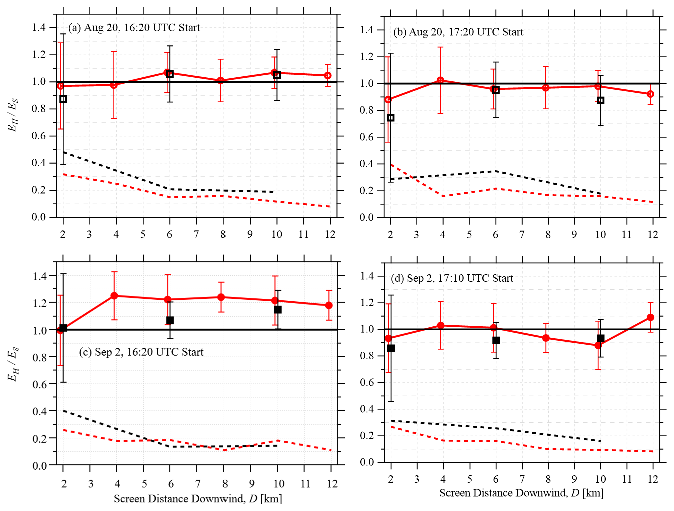
Figure 7 As Fig. 3 for the flights downwind of the small area sources. Error bars and dashed lines show one standard deviation (calculated from 10 flights).

For the small area sources (Fig. 7a–d), the variability between the flights is consistently reduced with distance from the source, ranging from 26 % to 48 % at D=2 km to between 8 % and 12 % at D=12 km. The variability of the large area source measurements is much lower and does not consistently decrease with D, with values ranging from 2 % to 13 %. The lower variation for the large area source is expected since the wide plume from such a large area would be much less susceptible to wafting and the smaller-scale variation due to local wind effects. This indicates that a single flight sampling a large area source shows substantially less uncertainty relative to a single flight sampling small area sources. For example, at D=6 km, the uncertainty in the estimate from a single flight (based on the variability between flights) is 20 % for the large area source, compared to 51 % for the small area sources (2.36σ, corresponding to the value of n_eff=8 for these cases, JCGM, 2008). Additionally, since D is defined as distance from the edge of the area source (as is necessary to sample the entire source area), emissions from the upwind side of the area source will have had more time to mix relative to the emissions from the downwind side of the are source. Hence, it would be expected that larger area sources have smaller uncertainties for similar D values relative to small area sources.

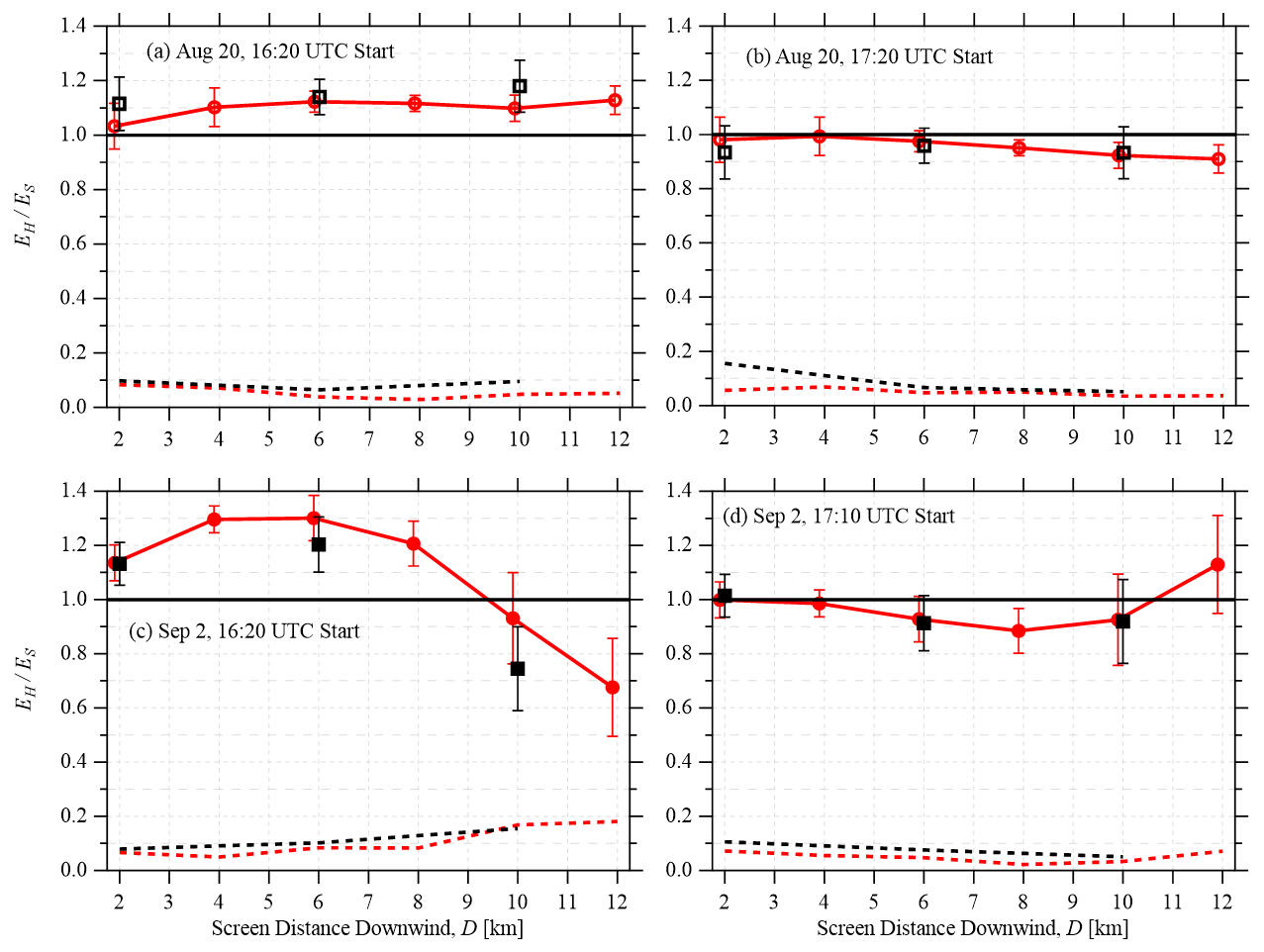
Figure 8 As Fig. 3 for the flights downwind of the large area sources. Error bars and dashed lines show one standard deviation (calculated from 10 flights).

Concentration profiles are shown in Fig. 4e–l from the instantaneous area source sampling, where they are compared to the extrapolation of a constant concentration below the lowest flight path. For the small area sources (Fig. 4e–h), the concentration is nearly constant below 150 m at D=6 km for 20 August, but it is overestimated by the constant extrapolation at D=6 km for 2 September. At D=10 km, the concentration is nearly constant for all except the 20 August 16:20 case, where it is overestimated by the extrapolation. For the large area source, the profiles for the 20 August flights (Fig. 4i–j) approach constant below the lowest flight path at D=6 km; however, at 10 km downwind the concentration increases toward the ground for the 16:20 flights. For the 2 September flights at 16:20 (for the large area source), the profiles (Fig. 4k) do not deviate from an exponential increase towards the surface at all distances, while for the 17:10 flights, they approach nearly constant at D=10 km (with a slight underestimation by the extrapolation). It would be expected that an underestimation due to extrapolation (most prominent for the 2 September 17:10 flights) would result in an underestimation of the emission rate for the non-instantaneous flights (relative to the instantaneous flights); however, this is not seen in Fig. 8c, where the instantaneous advection flux is lower than the non-instantaneous advection flux (which includes the extrapolation).

As with the flights sampling the stack sources, it is difficult to determine an optimized downwind distance for these flights. For the small area sources, the minimum distance with consistent emission estimation, minimum variability, and close to constant concentration below 150 m is D= 6 km; however, the non-constant concentrations below 150 m during the 2 September flights (at D=6 km) suggests that the optimized value of D may be further downwind in some circumstances. For the large area sources, there is little variation in the concentration profile shape with downwind distance and the variance between flights is relatively small and independent of downwind distance. For this source and these atmospheric conditions, we can suggest an optimum downwind distance of D=4 km. However, it is noted that, for both sources, the horizontal advection flux (E_H) differs significantly from the known emission rate (E_S), with factors between 0.96 and 1.22 for the small area sources (at D=6 km) and between 0.99 and 1.30 for the large area sources (at D=4 km). The overestimation could be associated with negative storage (release).

3.2.2 Optimizing Screen Flights for ΔZ

Using these optimal downwind distances (6 and 4 km), we investigate the change in estimated emissions with transect spacing, ΔZ using only the 16:20 flights. For the small area source (at D=6 km), there is no change in $E_{\mathrm{H}}/E_{\mathrm{S}}$ (≈1.06) with ΔZ for the 20 August flights (Fig. 9a); however, the variance between flights increases from 11 % at ΔZ=50 m to 19 % at ΔZ=200 m. For the 2 September flights, $E_{\mathrm{H}}/E_{\mathrm{S}}$ decreases with increasing ΔZ, from 1.29 to 1.02, and the variance is lower at ΔZ=50 m (10 %) and highest at ΔZ=100 m (20 %). These results suggest that the uncertainty due to variation between flights can be minimized with a 50 m spacing; however, the emission rate estimation for the 2 September flights at this spacing is high ($E_{\mathrm{H}}/E_{\mathrm{S}}=\mathrm{1.29}$). Increasing the spacing to 200 m will reduce the flight time by a factor of 4 but nearly doubles the uncertainty due to variation between flights.

The variation of $E_{\mathrm{H}}/E_{\mathrm{S}}$ and σ with ΔZ for the large area source (Fig. 9b) is similar to the variation seen for the small area source. For the 20 August flights, $E_{\mathrm{H}}/E_{\mathrm{S}}$ increases with ΔZ, from 1.08 at ΔZ=50 m to 1.15 at ΔZ=150 m and the variance increases from 6 % at ΔZ=50 m to 10 % at ΔZ=200 m. For the 2 September flights, $E_{\mathrm{H}}/E_{\mathrm{S}}$ decreases with increasing ΔZ, from 1.31 to 1.26, and the variance ranges from a minimum of 4 % at ΔZ=50 m to ∼7 % for other values. Similar to the small area source, the spacing is optimized (based on variation between flights) at 50 or 100 m but increasing the spacing to 200 m increases the uncertainty from 6 % to 10 % (20 August) or 4 % to 6 % (2 September), which could be acceptable depending on the required accuracy and the cost of flight time.

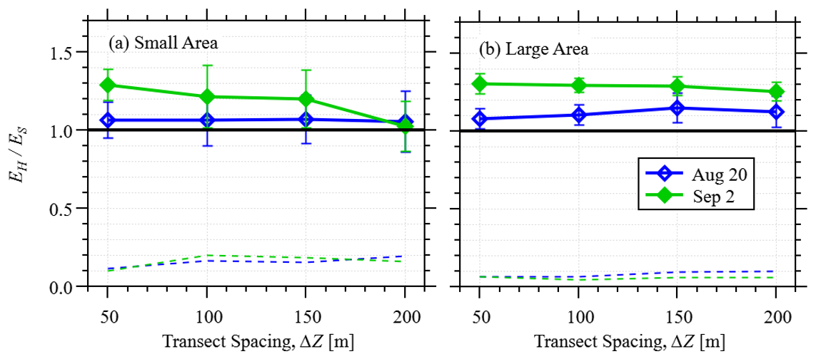
Figure 9 As Fig. 6 for the flights downwind of the small (a) and large (b) area sources for the flights starting at 16:20 only. 20 August shown as blue, open symbols, and 2 September shown as green, closed symbols.

3.2.3 Optimizing Screen Interpolation

We repeat the investigation of the interpolation described in Sects. 2.4.3 and 3.1.2 for the small and large area sources. Here we only investigate the kriging interpolation with the spherical variogram model, having demonstrated small differences between the different interpolation methods in Sect. 3.1.2. Results for the small area source are similar to the results for the stack sources shown in Fig. 10. Close to the source (D=2 km), there is overestimation in the interpolated concentration for z>150 m, and significant underestimation of the extrapolated concentration for z<150 m. Further from the source (D≥6 km), the average ratio (for each flight set) of interpolated to actual concentration ($<C_{\mathrm{K}}>/<C_{\mathrm{M}}>$) for z>150 m varies from 0.96 to 1.04, while the extrapolated concentration below 150 m shows significant errors (with $<C_{\mathrm{K}}>/<C_{\mathrm{M}}>$ as high as 1.22). In all cases, the variability between flights decreases with downwind distance, ranging from 4 % to 7 % for the z>150 m interpolation for D≥6 km. For the large area sources, there is much less error in the interpolation above 150 m, relative to the error in the interpolation from the stack or small area sources. Average values of $<C_{\mathrm{K}}>/<C_{\mathrm{M}}>$ range from 0.99 to 1.02, and the variability between flights is less than 4 % for all downwind distances. There is significant underestimation of the extrapolated concentration below 150 m, especially for the 2 September flight sets, which was previously demonstrated in Sect. 3.2.1 (e.g. Fig. 4k).

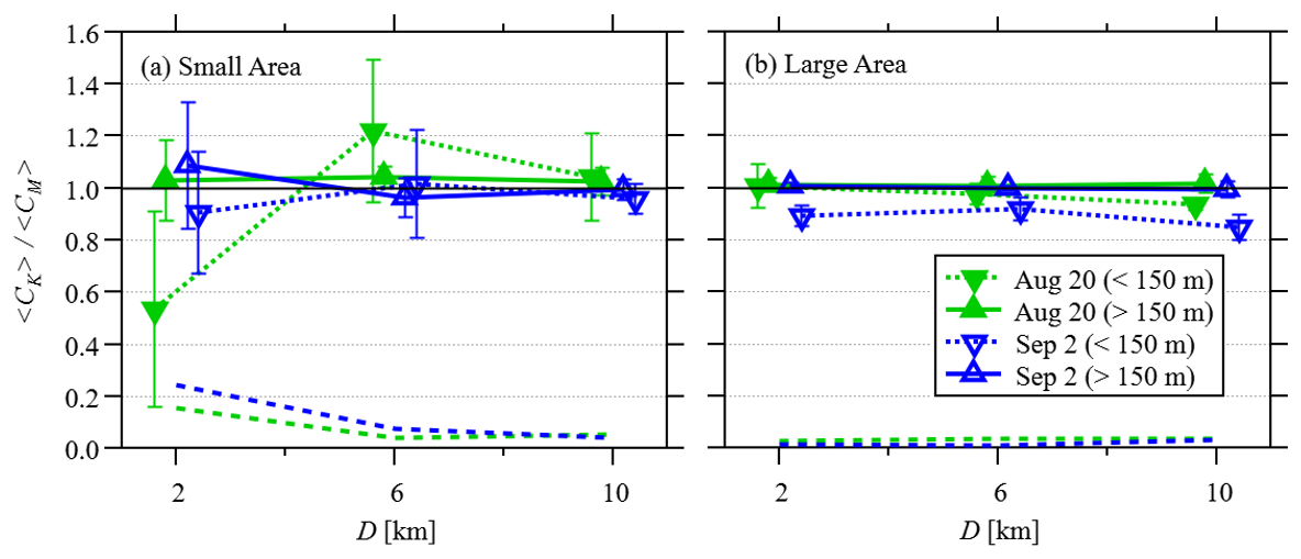
Figure 10 A comparison of average concentration from the instantaneous screens (at downwind distance, D) $<C_{\mathrm{M}}>$, to the average concentration from an interpolation of those flights with sparse sampling $<C_{\mathrm{K}}>$ downwind of area sources. The averages are separated into below (downward triangles with dotted line) and above (upward triangles with solid lines) 150 m, where the below 150 m concentrations are assumed constant (see Fig. 4). The markers are offset slightly for clarity. Results are shown for (a) the small area sources and (b) large area source, for the 20 August (green solid triangles) and 2 September (blue open triangles) 16:20 flight sets. The standard deviations of the 10 flights (σ) are shown as error bars, as well as dashed lines (for >150 m only).

3.3 Storage

We calculate the variability in the storage term (σ_S) for the volume defined by each flight configuration (3 sources, 6 downwind distances), for the two flight dates, as discussed in Sect. 2.7. The two dates investigated use the flight configurations for the flight sets starting on 20 August at 16:20 (Fig. 1a) and the flight sets starting on 2 September at 16:20 (Fig. 1c). The resulting variabilities in $S/E_{\mathrm{S}}$ as a function of D (using the average flight length for that flight set) are shown in Fig. 11. Generally, for the stack and small area sources, the variability in the storage term is minimum between D=6 and 8 km, while the variability in the storage term for the large area source increases with D. For the stack and small area sources, the higher σ_S at small D is likely because these flights take less time (typically 1 to 2 min) which leads to a higher variability between flights since each flight is a snapshot of a changing large-scale flow field. This effect is more pronounced for the stack sources, relative to the small area sources, and the effect is not seen for the large area sources, since there would likely be more variability in a thinner wafting plume from stacks or small area sources compared to the spread-out plume associated with a large area source. The higher σ_S at large D may be due to the larger volume enclosing the source and plumes, which encloses large-scale eddies and circulation, offsetting the reduced variability due to the longer flight durations.

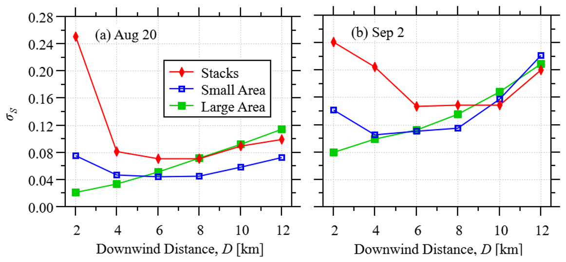
Figure 11 The variability (σ_S) in the storage term normalized by emission rate ($S/E_{\mathrm{S}}$) as a function of the downwind distance (D), from (a) 20 August 16:20 to 18:47 and (b) 2 September 16:20 to 18:09. The volumes are defined for the 3 source types (red line stacks, blue lines small area, green lines large area) and the 6 downwind distances (D=2 to 12 km).

The autocorrelation of the storage rate (S) time series (which is 147 min and 109 min long for the 20 August and 2 September dates respectively) gives a timescale of less than 3 min for all cases. Hence, we are 95 % confident that storage term for any one flight will be within ±2.03σ_S (35 degrees of freedom, JCGM, 2008). For the configurations investigated here, an optimal downwind distance of D=6 or 8 km gives σ_S between 4.4 % and 7 % for 20 August and between 11 % and 15 % for 2 September, suggesting an uncertainty as high as 14 % and 30 % respectively. This is in good agreement with the values of $S/E_{\mathrm{S}}$ reported in Fathi et al. (2021) (−3 % for the 20 August flights and −29 % for the 2 September flights) and those reported in Fathi et al. (2023) (up to 10.9 % for 20 August and −27.5 % for 2 September). For large area sources, the uncertainty associated with storage can be reduced to 4 % and 14 % (for 20 August and 2 September) by flying the screen closer to the source at D=2 km.

3.4 Scaling

Figure 12a and b compare the emission flux estimates and variation for all the sources for both dimensionalized downwind distance, D (Fig. 12a), and non-dimensionalized downwind distance, D^′ (Fig. 12b). As shown in Eq. (1), D^′ is normalized by the boundary-layer height (z_i). Here we use an average z_i value for each flight set but note that this value can vary significantly during the flights. For all August 16:20 flight set, the model value of z_i is constant (824 m). It then grows linearly during the 17:20 flight sets, from 867 m to 1315 m (for the 40-min duration of longest flights at D=12 km). During the 2 September flight sets, z_i increases from 528 m at 16:20 to 1078 m at 17:00 and then decreases from 1078 m at 17:10 to 952 m at 17:50. Hence, this normalization should be interpreted with some degree of caution. Although the variation is relatively small in most cases (more than 50 % of the flight sets show less than 5 % change in z_i during the flight durations), in some cases the increase in z_i can be up to 100 %.

Using these estimations of D^′, the results are not collapsed due to non-dimensionalization as substantial variation is seen in the results using either D or D^′. There is significant variability in the average values of $E_{\mathrm{H}}/E_{\mathrm{S}}$ for all sources over a wide range of D^′ values, and the results do not asymptote to a value of $E_{\mathrm{H}}/E_{\mathrm{S}}=\mathrm{1.0}$. For the large area sources, the standard deviation, σ (the variability between the 10 flights) is lowest for $D{}^{\prime }\le \mathrm{6}$, while for the stack and large area source flights, σ tends to decrease with D^′, but there is no apparent minimum or asymptotic D^′ value.

We also investigate the effect of non-dimensionalization on the accuracy of the constant concentration extrapolation below the lowest flight path. The average concentration below the lowest flight path $<C_{\mathrm{M}}>$ is calculated from the instantaneous flights (see Fig. 4) and this is normalized by the extrapolated concentration at the lowest flight path level, C(z_l), where z_l=150 m. When the results are non-dimensionalized, $<C_{\mathrm{M}}>/C\left(z_l\right)$ varies from 0.85 to 1.19 for $D{}^{\prime }\ge \mathrm{3}$, suggesting that the extrapolation should be within approximately 20 % beyond that distance. However, this analysis ignores the significant overestimation of $<C_{\mathrm{M}}>$ for the 20 August 17:20 stack flights at D=10 km (see Fig. 4b), and it is unclear what would happen at further downwind distances for that flight.

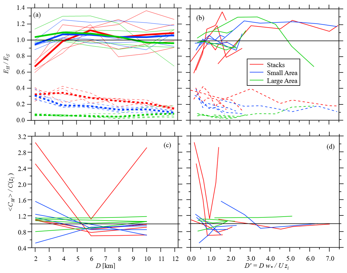
Figure 12 A summary of the results shown in Figs. 3, 4, 7, and 8, compared to both downwind distance D (a, c), and non-dimensionalized downwind distance, D^′ (b, d). Panels (a) and (b) show the ratio of estimated advection flux, E_H, to the known emission rate, E_S, and the standard deviation of the ratio, σ. In Panel (a), the thicker line is the average of all 4 flight times. Panels (c) and (d) show the ratio of average concentration, $<C_{\mathrm{M}}>$, below the lowest flight level (z_l=150 m) to the constant concentration, C(z_l), extrapolation (see Fig. 4).

4 Conclusions

The results of this study demonstrate that emissions estimates can be substantially varied under different conditions. This reinforces the importance of storage and release discussed in Fathi et al. (2021, 2023). A vertically moving (rising or falling) plume may also lead to under- or over-estimation of the emissions for the non-instantaneous flight, although this would not explain under- or over-estimation in the instantaneous flights. Further uncertainty is introduced by the sparse interpolation, especially close to the source, with uncertainties as high as 132 % for stack sources or 57 % for small area sources (both at D=2 km). Further from the source (D≥6 km) the uncertainty associated with interpolation is much smaller (≤17 %).

When all the different flight times are averaged, the storage/release conditions tend to cancel and the average E_H values are within 12 % of E_S for a downwind distance of 4 km or more. Hence, based on the average estimate of $E_{\mathrm{H}}/E_{\mathrm{S}}$ alone for the cases studied here, a screen at a downwind distance of 4 km or more provides the same level of accuracy for the three types of sources investigated here (i.e. elevated stacks, small surface area sources, or a large surface area source).

However, variability between individual flights is a very large source of uncertainty. This variability is likely due to changes in storage/release over the flight times, since similar variability is seen in instantaneous results. At a downwind distance of 4 km, for elevated stack sources, this variability between flights can be as much as σ=42 %, which suggests an uncertainty of 99 % (at a 95 % CI) in that particular case. At the same distance, variability for the surface area sources is much less (σ=25 % for small area sources, and 7 % for the large area source). The variability between flights tends to decrease with increasing downwind distance. For the stack and small area sources, σ reaches half the D=4 km value between D=10 and 12 km. However, flight time also increases with downwind distance. For the case of the stack sources, the screen at 12 km takes 3 times as long to complete as the screen at 4 km (since L=D for the smokestack screens). Hence, 3 flights can be flown at D=4 km in the same time it takes to fly one flight at D=12 km. Taking the average of these 3 flights (assuming the results are independent), would reduce the uncertainty by a factor of 0.58 ($\mathrm{1}/\surd \mathrm{3}$). Hence, comparable accuracy can be achieved by taking multiple flights closer to the source relative to a single flight further downwind. In these cases (for the conditions investigated here), results show that estimates can be improved and variability reduced by completing multiple screens in opposite directions (e.g. up then down). For large area sources, the variation is small and reaches a minimum (average σ=5 %) at D=8 km. For this source type, increasing the downwind distance of the screen does not reduce uncertainty due to variability between flights. Generally, in real-life conditions, any reduced uncertainty due to flying further downwind from source must be balanced against increased relative uncertainty due to spatial and temporal variability in the concentration, especially for pollutants with high background concentrations (due to the weaker concentration signal as the plume disperses).

For elevated stack sources, the results show that, for these cases, reducing the transect spacing below 100 m does not offer any benefits in emission estimation, but increasing the space beyond 150 m can increase uncertainty and modify the E_H estimates. For the area sources we investigate here, the variability between flights is minimized with a transect spacing of ΔZ=50 m. For the small area sources we investigate here, increasing the spacing to 200 m (reducing flight time by a factor of 0.25) doubles the uncertainty, while for the large area source we investigate here, increasing the spacing to 200 m increases the uncertainty by a factor of ∼1.5. As with the optimization of downwind flight distance, multiple flights with a larger transect spacing may result in similar uncertainties compared to a single flight at smaller transect spacing.

Analysis of the storage term for the various flight configurations investigated here suggest that the uncertainty associated with the storage term is minimized at downwind distances between D=6 and 8 km for stack and small area sources. For the flights on 20 August this uncertainty is as high as 14 %, while for flights on 2 September it is as high as 30 %, demonstrating a strong dependence on meteorological conditions, likely due to non-stationary wind and stability conditions. For the large area source, the uncertainty is minimal close to the source (D=2 km), and is estimated here as 4 % and 14 % for the flights on 20 August and 2 September, respectively.

These results further demonstrate that one of the most substantial sources of error in the emissions estimate is due to the extrapolation of the results between the surface and the lowest flight path level (as outlined by Gordon et al., 2015 and Conley et al. 2017 for example). Extrapolation error is most significant close to the source, as would be expected, but it can be surprisingly persistent further downwind, in one flight case (for the stack sources), overestimating the concentration below 150 m by a factor of 3 at D=10 km. For the area sources, the extrapolation error is less than 30 % for distances of 4 km or greater. Non-dimensionalization of the results suggests that the extrapolation error is within 20 % for non-dimensional distance of $D{}^{\prime }\ge \mathrm{3}$, with the caveat that more results at this distance are required to confirm this result. Although gravitational settling of particles or deposition (of gas or particles) to the surface could modify the concentration profiles, especially near the surface, these results generally emphasize the need to constrain aircraft measurements with coincident surface or near-surface measurements whenever possible. Tests with a mobile vehicle sampling at ground level (Sect. S1) suggest that variability between flights can be reduced by as much as 6 % and underestimation of the emissions close to the source (where the plume is typically lower) is eliminated in the case investigated here. Substantial improvements in emission estimation accuracy could potentially be achieved with UAV or remote sensing (e.g. lidar) sampling beneath the aircraft.

The results demonstrate that it is difficult to provide a single optimized distance and transect spacing given the variability of conditions and the effects of storage and release. However, the results suggest that emission rate retrieval could potentially be improved by accompanying any flight campaign with a strong modelling effort, at least to help with the estimation of storage uncertainty and the understanding of plume dynamics and behaviour.