Leveraging machine learning techniques and SEVIRI data to detect volcanic clouds composed of ash, ice, and SO₂

Volcanic clouds can influence the climate and pose a serious threat to air transportation. Detecting and distinguishing them from meteorological clouds is particularly challenging because they often are composed of water vapor and ice particles, along with ash and gases. This study presents a neural network (NN) model for the detection of volcanic clouds composed of ash, ice, and SO₂, applied to data acquired by the Spinning Enhanced Visible and InfraRed Imager (SEVIRI) satellite instrument. A dataset of 1259 SEVIRI images related to Mount Etna volcano (Italy) eruptions spanning from 2020 to 2022, as well as 2024, was considered. The NN model, based on a multi-layer perceptron (MLP), was developed using 13 features, including thermal infrared channels and brightness temperature differences (BTDs). A post-processing step based on a plume-tracking algorithm and a Non-Local means filter was implemented to improve the performance of the NN model. The model was validated using three eruptive events that were not included in the training phase, achieving an overall balanced accuracy of up to 92.0 %. The validation results also showed that the model successfully detected 66.0 %, 48.5 %, and 84.1 % of the observed volcanic cloud (VC) pixels in the three analysed validation events, respectively. In addition, only 7.7 %, 4.0 %, and 21.9 % of the detected VC pixels corresponded to false alarms for the respective events. Thus, the model demonstrates the capability to detect volcanic clouds even under complex conditions of high meteorological cloud cover. The results are promising for the automatic detection of volcanic clouds, including those containing ice and SO₂, as well as for improving volcanic cloud retrieval processes.

1 Introduction

Volcanic eruptions can release vast amounts of ash particles and gases into the atmosphere and form volcanic clouds that pose serious risks to aviation (Alexander, 2013; Prata and Rose, 2015), to human health (Stewart et al., 2021), to the environment and the climate (Jenkins et al., 2023; Marshall et al., 2022). Detecting volcanic clouds is crucial for aviation safety and assessing their potential impact, for height estimation methods, retrieval algorithms, and dispersion models. Nonetheless, the detection of volcanic clouds continues to pose a significant challenge (Prata et al., 2022).

The use of satellite imagery has been essential for advancing volcanic cloud detection capabilities, as they can collect information over large areas and across a broad range of wavelengths. The widely recognized method for detecting volcanic clouds containing ash is the Brightness Temperature Difference (BTD) technique, based on the difference between the channels centered around 11 and 12 µm, which was postulated by Prata (1989a, b). It exploits the reverse absorption phenomenon that occurs in the 11 and 12 µm wavelengths range. In this spectral region, the volcanic ash signature is opposite to that of water and ice, which are the primary components of meteorological clouds. Specifically, ash absorbs more energy in the 11 µm band than in the 12 µm band, whereas water and ice absorb more energy in the 12 µm band than in the 11 µm band. As a result, the BTD is normally negative in the presence of ash and positive in the presence of meteorological clouds. However, there are some well-known circumstances in which the BTD method fails, leading to false positives and false negatives during the detection (Pardini et al., 2024; Prata et al., 2001). Over the last two decades, many studies have focused on improving and overcoming the limitations of the BTD method by presenting more sophisticated approaches, such as water vapor correction (Corradini et al., 2008; Yu et al., 2002), methods using multiple channels for daytime detection (Ellrod et al., 2003; Pavolonis et al., 2006; Pergola et al., 2004), principal component analysis (Hillger and Clark, 2002), β ratios (Pavolonis et al., 2015a, b), and machine learning techniques (Gray and Bennartz, 2015; Petracca et al., 2022; Picchiani et al., 2011, 2015; Piscini et al., 2014; Romeo et al., 2023; Torrisi et al., 2022, 2024).

Despite all these approaches, there is still a need for reliable methods that can automatically detect volcanic clouds, particularly when they contain a mixture of ash, ice, and SO₂. The detection of SO₂ in volcanic clouds can be effectively achieved using the 7.3 and 8.6 µm wavelength bands, where SO₂ exhibits strong absorption features. Although the 7.3 µm band shows stronger absorption, it is also influenced by significant water vapor interference (Corradini et al., 2009; Pavolonis et al., 2020). Thus, by combining data from both bands, it is possible to enhance the reliability of SO₂ detection.

Moreover, the presence of ice in volcanic clouds is tricky, as it masks the spectral response of ash (Rose et al., 1995). Since ice has an opposite spectral response to ash, it produces a positive BTD for volcanic clouds when present, resulting in false negatives and complicating the accurate detection of volcanic clouds (Guerrieri et al., 2023; Gupta et al., 2022; Mayberry et al., 2002; Prata et al., 2020; Rose et al., 1995, 2003). False negatives in detection are caused by ice formation through nucleation processes occurring within volcanic clouds (Durant et al., 2008), which can be either homogeneous (Prata et al., 2020) or heterogeneous (Seifert et al., 2011). In the latter case, volcanic ash particles act as ice nuclei (Wang, 2013).

The limited understanding of nucleation processes within volcanic clouds underlines the need for accurate detection methods in these circumstances (Durant et al., 2008; Schill et al., 2015). This need aligns with the requirements of the International Civil Aviation Organization (ICAO), which expects all Volcanic Ash Advisory Centers (VAACs) to provide Quantitative Volcanic Ash (QVA) information by late 2027 (ICAO, 2021, 2024). However, obtaining accurate QVA information relies, though not exclusively, on precise detection methods (Guerrieri et al., 2023; Prata et al., 2022).

With the purpose of exploring the detection of volcanic clouds containing a mixture of ash, ice, and SO₂, this paper focuses on leveraging machine learning techniques and data from the Spinning Enhanced Visible and InfraRed Imager (SEVIRI) instrument aboard the Meteosat Second Generation (MSG) geostationary satellite. As a case study, the eruptive activity of Mount Etna (Italy) was analysed for the periods 2020–2022 and 2024, where the events generated volcanic clouds with varying combinations of constituents (Guerrieri et al., 2023), offering a unique opportunity to investigate the detection challenge. The results provide insights into the detection of ash, ice, and SO₂ within volcanic clouds and show promise for the automatic detection and retrieval of volcanic clouds in near-real time.

This paper is organised as follows: Sect. 2 describes the case study, the SEVIRI satellite instrument characteristics and how the training dataset was built. Section 3 covers the development of the NN model and the different steps involved. The results are presented in Sect. 4 and the discussion in Sect. 5. Final conclusions are drawn in Sect. 6.

2 Materials and methods

This section presents a description of the case study, the SEVIRI data and how the training dataset was built.

2.1 Case study

As a case study, the Etna eruption activity between 13 December 2020 and 21 February 2022 was selected. During this period, Etna volcano produced 66 lava fountain episodes from the new South-East crater. Despite their short duration (an average time of about two hours; Calvari and Nunnari, 2022), they produced a strong impact on human life, environment, and air traffic.

These paroxysmal events produced large Volcanic Clouds Top Heights (VCTH) ranging from 4 to 13 $\mathrm{km}\mathrm{a}.\mathrm{s}.\mathrm{l}.$ Based on VCTH, the entire period can be approximately divided into three main time ranges characterized by average VCTH values of 9 km (from 13 December 2020 to 19 March 2021), 6 km (from 24 March 2021 to 17 June 2021) and 10 km (from 19 June 2021 to 21 February 2022). Most of these volcanic clouds were composed of ash, ice, and SO₂, with the ice content being greater than the ash. The ice generation was related not only to the volcanic cloud height but also to the season: during the summer, with almost the same plume height, the amount of ice was lower than that observed in winter (Guerrieri et al., 2023). The presence of ice in most volcanic clouds during this period makes it an interesting case study for exploring the challenges associated with volcanic cloud detection.

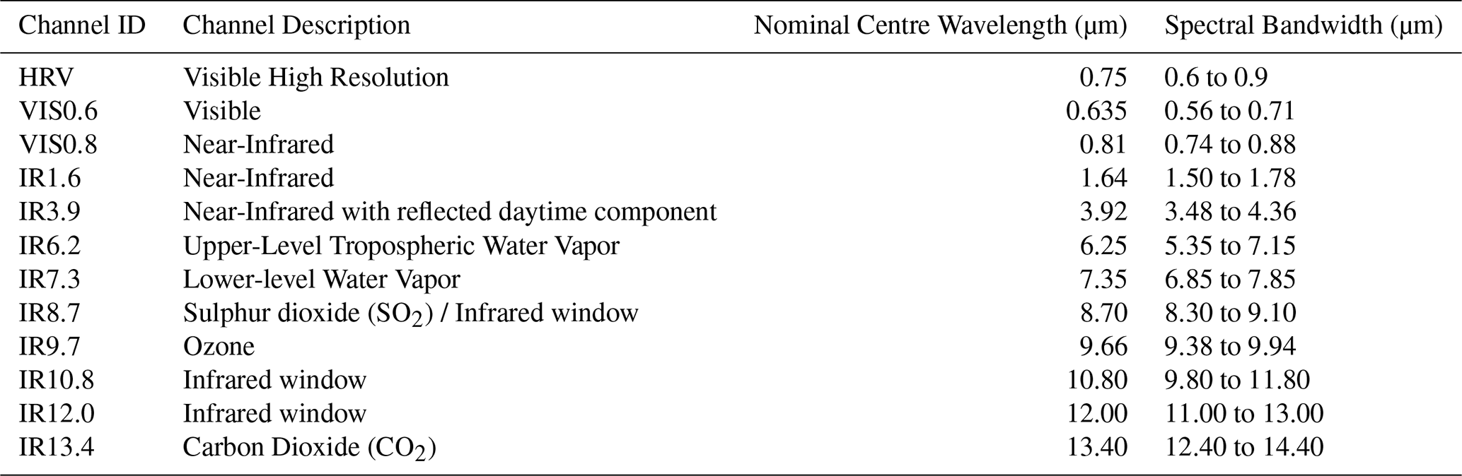
Table 1 Spectral channels description of the Spinning Enhanced Visible and InfraRed Imager (SEVIRI) instrument.

2.2 Satellite data

Data from the Spinning Enhanced Visible and InfraRed Imager (SEVIRI) instrument aboard the Meteosat Second Generation (MSG) geostationary satellite, specifically from the Meteosat-10 series orbiting at a 0° longitude, was considered in this work. The SEVIRI instrument can produce an image of the Earth's full disk every 15 min in 12 different spectral channels ranging from visible to infrared, with a nominal spatial resolution of 3 km × 3 km (1 km² for High-Resolution Visible channel) at the sub-satellite point (EUMETSAT, 2017). The SEVIRI's channel description and their nominal centre wavelengths are shown in Table 1. All the SEVIRI data used in this work were acquired in near real-time using the Multimission Acquisition SysTem (MAST), which was developed at Istituto Nazionale di Geofisica e Vulcanologia - Osservatorio Nazionale Terremoti (INGV-ONT). The MAST system uses EUMETCast dissemination service for the near real-time delivery of satellite data and products (Stelitano et al., 2023).

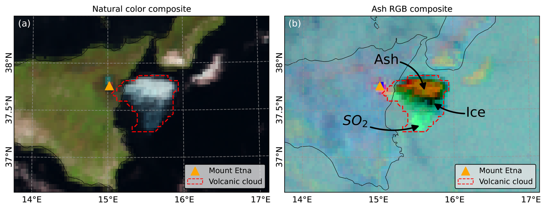
Figure 1 A volcanic cloud containing a mixture of ash, ice, and SO₂ on 19 February 2021 at 10:15 UTC, captured by SEVIRI-MSG. (a) Natural color composite with an overlaid hand-drawn volcanic cloud boundary (©EUMETSAT SEVIRI MSG, CC BY 4.0). (b) Same as (a) but showing the ash RGB composite. The cloud's regions where ash, ice, and SO₂ are present have been highlighted with a mask boundary (©EUMETSAT). Satellite data were processed by the authors from EUMETSAT Meteosat-10 SEVIRI Level 1.5.

An example of a volcanic cloud captured by SEVIRI from 19 February 2021 at 10:15 UTC is displayed in Fig. 1. This volcanic cloud is composed of a mixture of ash, ice, and SO₂. The natural color composite, created by assigning the IR1.6, VIS0.8, and VIS0.6 channels to the red, green, and blue color beams, respectively, is shown in Fig. 1a, where the volcanic cloud appears as a bright white cloud, similar to the surrounding meteorological clouds. By contrast, the volcanic cloud shown in Fig. 1b is well distinguished in the Ash RGB composite (Ash RGB Quick Guide | EUMETSAT – User Portal, 2025), which uses the thermal infrared channel. In this latter figure, generated by visualizing the channel differences IR12.0 − IR10.8 and IR10.8 − IR8.7 in the red and green color beams, respectively, and the IR10.8 channel in the blue beam, the constituents of the volcanic cloud are clearly identifiable: ash appears in shades of brown, ice in dark blue, and SO₂ in green color.

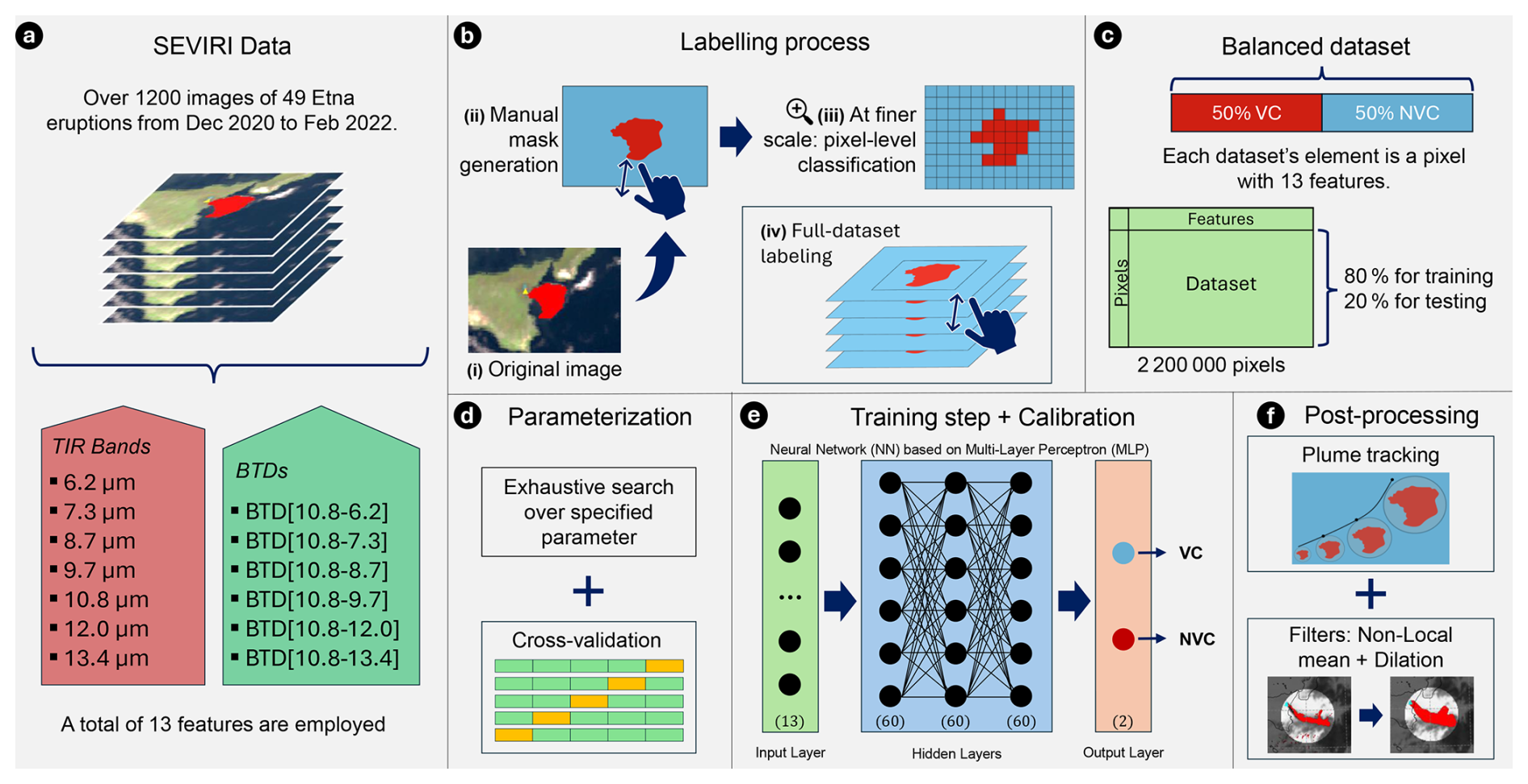
Figure 2 Model development overview. (a) SEVIRI data and features information. (b) Labelling workflow. (c) Dataset composition and division. (d) Hyperparameter tuning. (e) Training. (f) Postprocessing.

2.3 Dataset

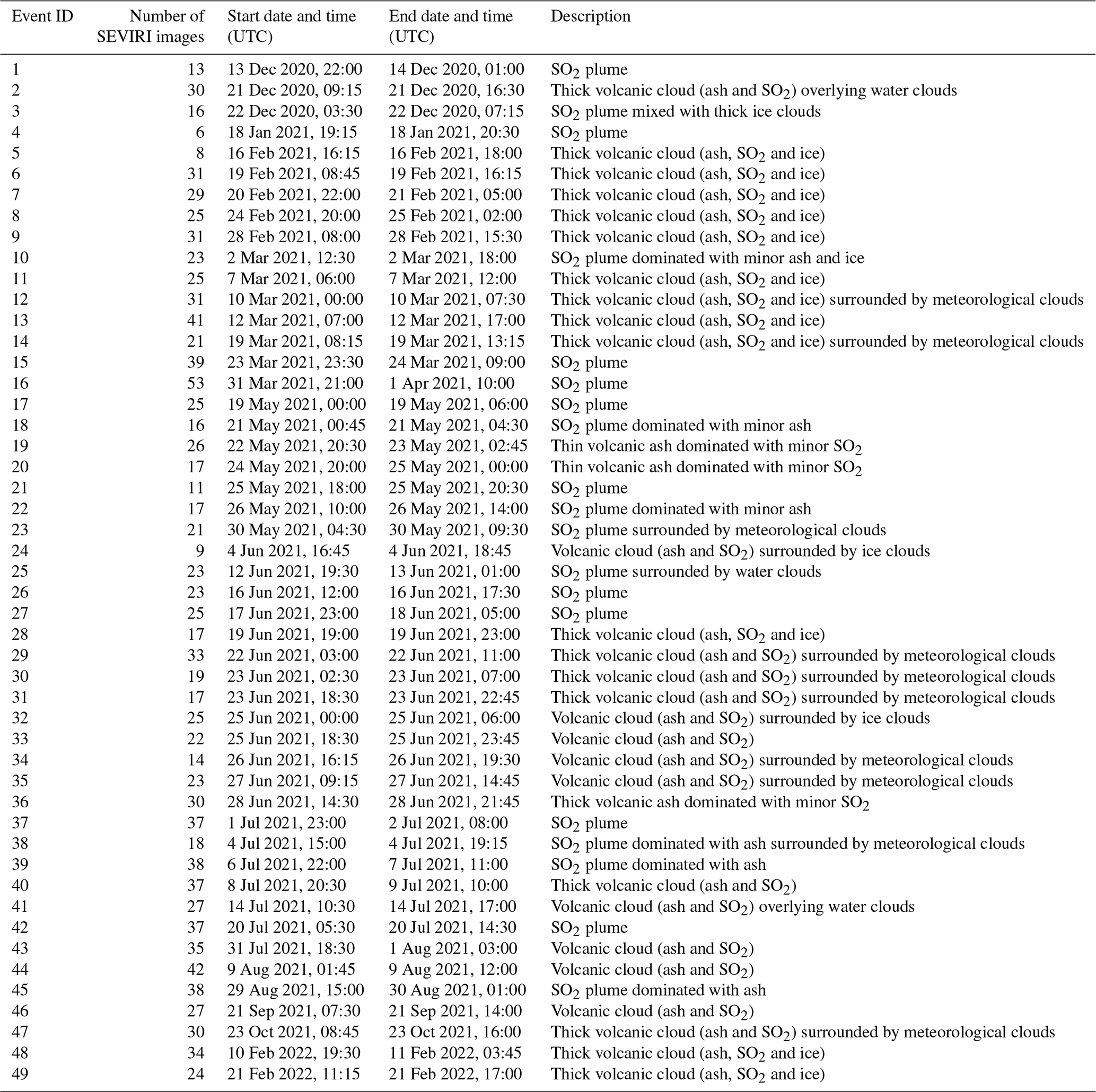
The dataset was generated from 1259 SEVIRI images covering 49 eruptive Etna events between December 2020 and February 2022 (see Fig. 2a). Overall, the dataset represents a comprehensive compilation of eruptive events, covering a wide range of volcanic cloud conditions. These events include SO₂ plumes, SO₂ dominated plumes containing minor ash components, and volcanic clouds composed of ash and SO₂. The dataset also includes highly challenging cases in which the volcanic clouds were composed of ash, SO₂, and ice, sometimes occurring under clear-sky conditions surrounding the volcanic cloud, and in other cases in the presence of meteorological clouds surrounding or mixing with the volcanic cloud. Table A1 provides a detailed description of the SEVIRI images employed to generate the dataset, including the number of images, the time range for each event, and a brief comment describing the composition of the volcanic cloud during each eruptive event.

All images were manually analysed in order to create a plume mask for each one; this step, generally known as the labelling process (see Fig. 2b), was also used in Guerrieri et al. (2023) to estimate the total masses of ash, ice, and SO₂. Figure 1 also presents an example of a plume mask. The manual plume mask generation generally provides the most accurate volcanic cloud detection, but it is a time-consuming process that requires expert interpretation. Despite the expertise of a human operator, some challenging events remain difficult to discriminate. This is particularly true when volcanic clouds are surrounded by meteorological clouds, making the identification of plume mask boundaries more uncertain. In such cases, the human operator tends to adopt a conservative approach, generating a smaller plume mask that includes only pixels with strong evidence of volcanic cloud presence. Consequently, the most ambiguous pixels were intentionally excluded from the manual plume mask, with the aim of allowing the NN model to learn how to discriminate these challenging events during the prediction phase.

In this work, the detection of volcanic cloud using SEVIRI data is analysed as a pixel-scale classification (see Fig. 2b(iii)). Thus, the dataset includes information from more than 2 200 000 pixels, organized in two balanced classes: 50 % belonging to the Volcanic Cloud (VC) class and the other 50 % to the Non-Volcanic Cloud (NVC) class, as indicated in Fig. 2c. The original dataset was highly imbalanced, containing 0.3 % VC pixels and 99.7 % NVC pixels. All VC pixels were retained, while NVC pixels were randomly sampled to obtain the final balanced dataset. The VC class refers to volcanic cloud pixels containing ash, SO₂, ice, or any combination of these components, whereas the NVC class refers to pixels associated with meteorological clouds, land surfaces, sea surfaces, and other non-volcanic features.

Among the pixel features that comprise the dataset are the thermal radiances from seven spectral channels, corresponding to the thermal-infrared region (6–14 µm) as detailed in Table 1. Selecting these spectral channels enhances model flexibility, allowing application both during the day and at night with a unique NN model. In the dataset, the thermal radiance from each channel is expressed as Brightness Temperature (BT) in Kelvin (K). In addition, several channel combinations were applied to derive six new features, known in the literature as Brightness Temperature Difference (BTD) including the traditional BTD between the channels centered around 11 and 12 µm. These new features are BTD[10.8–12.0], BTD[10.8–8.7], BTD[10.8–13.4], BTD[10.8–6.2], BTD[10.8–7.3] and BTD[10.8–9.7]. Thus, a total of 13 features are included in the dataset (as indicated in Fig. 2a), all serving as input variables for the neural network model. The balanced dataset is accessible in (Naranjo et al., 2026), where additional details regarding its spatial and temporal coverage are provided.

3 Model development

This section presents the development of the neural network model including the hyperparameter tuning, training and validation phases. Using the previously built balanced dataset a neural network (NN) model based on a multi-layer perceptron (MLP) with a feed-forward architecture was implemented to perform the detection of volcanic clouds. This architecture was chosen due to its efficiency in handling large volumes of data with both accuracy and speed, as well as its ability to incorporate a priori knowledge and realistic physical constraints into the analysis (Atkinson and Tatnall, 1997).

Here, it is worth defining the convention adopted for the datasets used in the development and validation of the model. For the hyperparameter tuning and training phases, the balanced dataset was divided into training and testing sets. The training set was used to fit the model and support the hyperparameter tuning process, whereas the testing set was used to evaluate the generalization performance of the model and assist in its calibration. In addition, a validation dataset, composed of data from three eruptions not previously seen by the model, was used for independent validation. These data were not included in the balanced dataset. Further details of the neural network model are provided in the following subsections.

3.1 Hyperparameter tuning phase

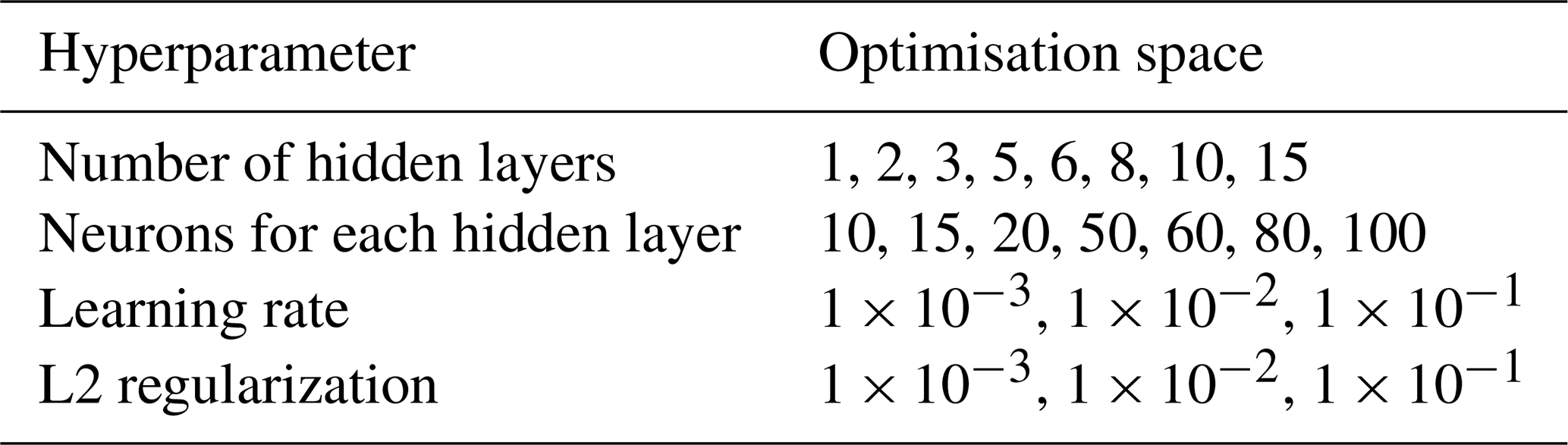
To determine the most suitable configuration for the NN model, a hyperparameter tuning phase was carried out. During this step, the hyperparameters listed in Table 2 were optimised using the search space specified in the table's right column. This process combined exhaustive search with a 5-fold cross-validation strategy (k=5) (Ojala and Garriga, 2010), evaluating all possible combinations within the defined optimisation space. Moreover, the balanced dataset (50 % VC and 50 % NVC, totalling 2.2 million pixels) was split into 80 % for the training set and 20 % for the testing set, in accordance with the proportions commonly employed in the literature (Sun et al., 2022). The split was performed using random sampling with a stratified strategy. This stratified approach ensures that the training and testing sets contain approximately the same proportion of samples from each class (VC and NVC) as the balanced dataset.

Table 2 List of hyperparameters and optimisation space used in the tuning phase.

During the hyperparameter tuning phase, both the classification accuracy and the average time required for the NN model to perform a single classification were considered. A trade-off was therefore established between achieving a training accuracy of 96.0 % and maintaining an average inference time of approximately 1.5 s per classification. The complete hyperparameter tuning results are provided in the Supplement, while the final selected hyperparameter combination is reported in Table 3 (Sect. 3.2, Training phase). Using these hyperparameters, the evaluation metrics obtained for the testing set were 95.0 % accuracy, 98.6 % precision, and 91.3 % recall (see Sect. 3.5 for the definition of these metrics).

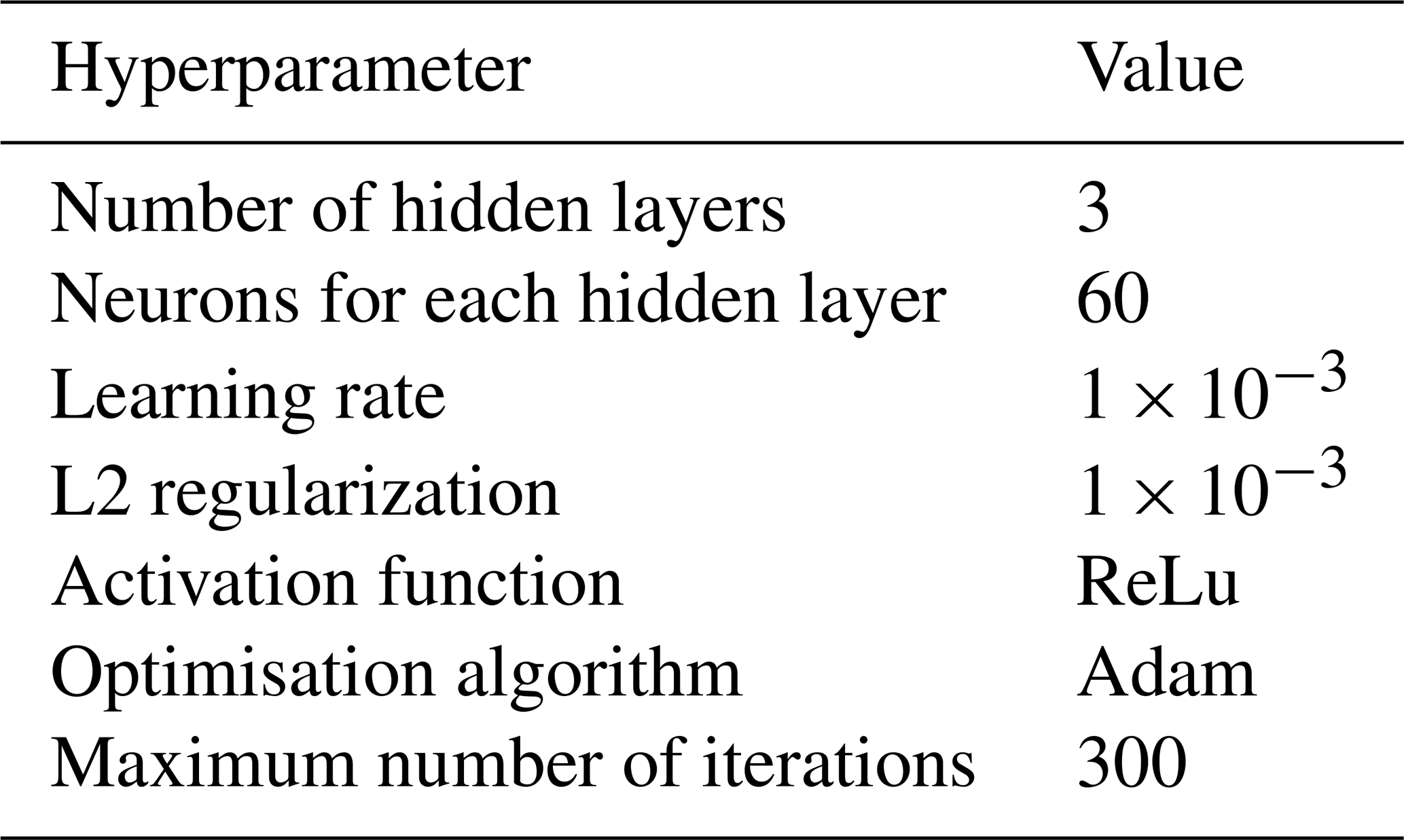
Table 3 Values of the hyperparameters used to train the final neural network model.

3.2 Training phase

During the training phase, the dataset was also split into 80 % for the training set and 20 % for the testing set, as in the hyperparameter tuning phase. Additionally, the data for each feature was independently standardized by removing the mean and scaling to unit variance, the process is also known as Z-score normalization. In this standardization step, data from both classes (VC and NVC) were included to calculate the mean and standard deviation for each feature. Standardization is an important requirement for NN models, as it generally improves their performance (Pinheiro et al., 2025).

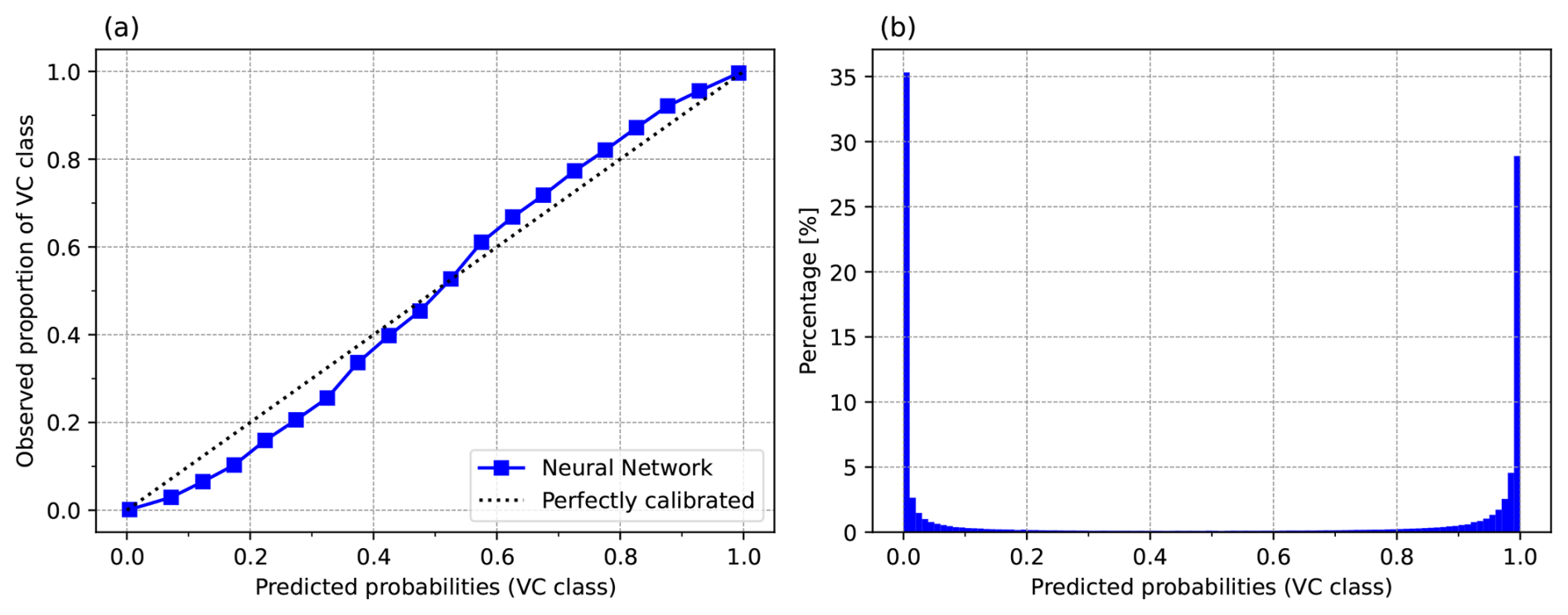
Figure 3 Reliability diagrams for the calibrated neural network model. (a) Calibration curve showing the predicted and observed probabilities for the testing set. (b) Histogram showing the distribution of the predicted probabilities for the testing set.

The NN model was trained using three hidden layers, each containing 60 neurons, as presented in Table 3. The learning rate and L2 regularization hyperparameters were both set to 1 × 10⁻³, based on the results obtained during the hyperparameter tuning phase. The activation function used was the Rectified Linear Unit (ReLU), which is the standard activation function for NN models based on MLPs (Braga-Neto, 2020; Yang, 2019). For the optimisation algorithm, the Adaptive Moment Estimation (Adam) method was applied, due to its computational efficiency and robustness in the training of models using large datasets (Kingma and Ba, 2014). Finally, the maximum number of training iterations was set to 300 and an early stopping strategy was implemented, whereby the training process was terminated when the model performance no longer improved between successive iterations.

In addition, the NN model was calibrated. When the model performs a classification, the output corresponds to the probability associated with the respective class, with values close to zero indicating the NVC class and values close to one indicating the VC class. However, the raw output probabilities are not inherently calibrated and may provide unreliable estimates of the true class probabilities. For this reason, a calibration procedure was incorporated into the training pipeline, enabling the predicted probabilities to be interpreted as the model's confidence that a given pixel belongs to a specific class (Niculescu-Mizil and Caruana, 2005).

The model's confidence specifically depends on the dataset on which it was trained, which in our case corresponds to the balanced dataset. For the calibration, the testing set (20 % of the balanced dataset) was used to train an additional calibrator model. This calibrator learned to map the raw output probabilities (p_raw) of the NN model to a calibrated probability (P_cal). In practice, the calibrator predicts the conditional event probability P(prediction=VC|p_raw). Therefore, the calibrated probabilities can be interpreted as confidence level.

The P_cal (depicted in Fig. 3a) is estimated by fitting an isotonic regression model using the NN raw output probabilities and the corresponding true labels from a testing set. The model learns the relationship between the raw probabilities and the observed probabilities (Guo et al., 2017; Niculescu-Mizil and Caruana, 2005). The calibrated probability for a new prediction is then obtained by applying the learned isotonic mapping to the NN model's raw output probabilities.

The calibration curve for the trained NN model is shown in Fig. 3a, where the y axis represents the observed proportion of VC class pixels in the testing set, whereas the x axis represents the predicted probabilities for these pixels. The calibration curve was generated by binning predicted probabilities and then plotting the mean predicted probability in each bin against the observed proportion of VC class pixels (Bröcker and Smith, 2007).

As shown in Fig. 3a, the NN model exhibits a slight tendency to overestimate low probabilities and underestimate high probabilities. For example, according to the Fig. 3a, among all pixels in the testing set predicted by the NN model with probability 0.80, more than 80 % actually belong to the VC class. However, the overall calibration performance is good, as can be seen in Fig. 3b. This figure presents the distribution of predicted probabilities, showing that for the VC class, most probabilities are concentrated at low (less than 0.2) and high (greater than 0.8) values. This symmetric and bimodal distribution indicates that only a small number of ambiguous probability values are present, which is a desirable characteristic of a well-calibrated classifier. Based on these results, a pixel will be classified as VC when the calibrated probability is higher than 0.8.

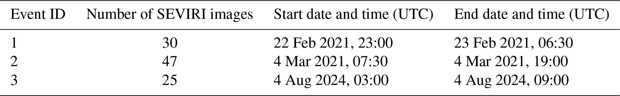
Table 4 List of events and SEVIRI images included in the validation dataset.

3.3 Validation phase

To validate the performance of the NN model, three sequences of SEVIRI images were selected, each corresponding to an eruption the model had not previously encountered during the training phase. The events are listed in Table 4, comprising two from 2021 and one from 2024. The SEVIRI images for the 2024 event were captured by the Meteosat-11 satellite. In contrast, the images for the 2021 events were captured by the Meteosat-10 satellite, the same satellite used to acquire the data for the training phase. All three events represent challenging scenarios in which the volcanic clouds are composed of ash, ice, and SO₂, with the last event additionally characterised by the mixing of the volcanic cloud with meteorological clouds.

Each SEVIRI image sequence was also manually analysed to create a plume mask for each image, following the same labelling process carried out for the training dataset (as illustrated in Fig. 2a). The plume masks are used as the observed data to compare the predictions of the NN model and assess its performance through conventional evaluation metrics such as accuracy, precision, recall, F1-score and confusion matrix (Fawcett, 2006; Rainio et al., 2024).

3.4 Plume tracking and non-local mean filter

The raw output of the NN model is subsequently post-processed using a plume tracking method and a non-local (NL) mean filter. This two-step post-processing procedure is designed to reduce false positive detections (see Fig. 2f). A similar methodology was previously presented by Pavolonis et al. (2018), who introduced the Cloud Growth Anomaly (CGA) technique.

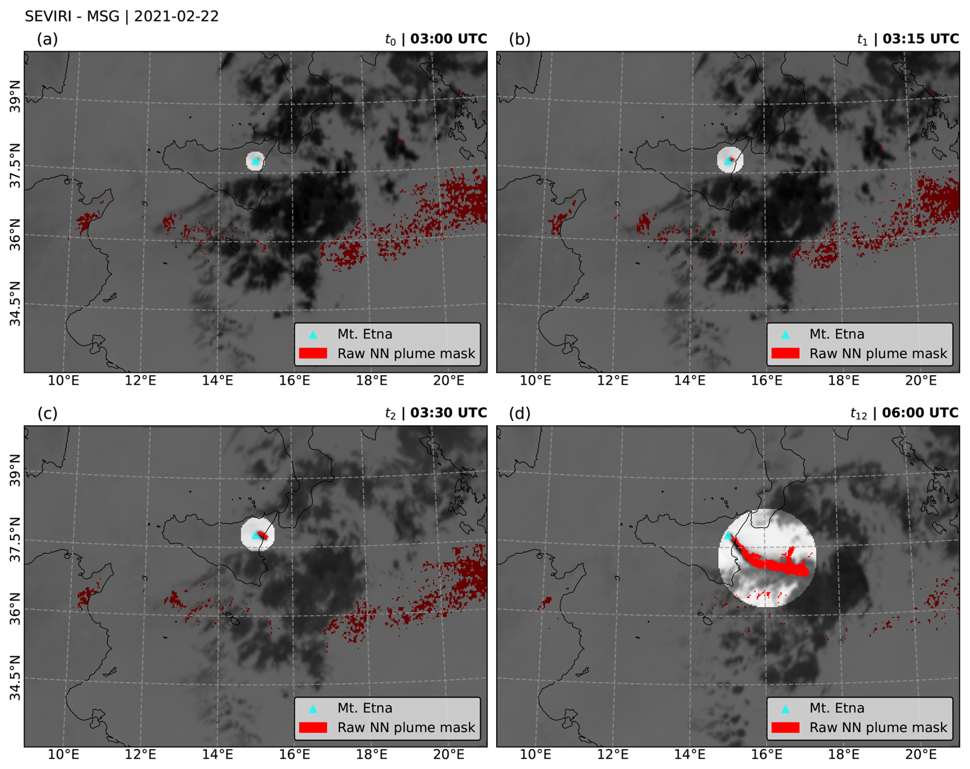
Figure 4 Example of plume tracking from the 4 August 2024 eruption of the Mount Etna. (a) At t₀ = 03:00 UTC, a volcanic cloud (VC) object was not yet detected within the 25 km radius around the volcano. (b) At t₁ = 03:15 UTC, the first VC object is detected, which is the triggering event. (c) At t₂ = 03:30 UTC. (d) At t₁₂ = 06:00 UTC, the dispersed VC tracked by the algorithm.

The tracking algorithm developed in this work is initialized (t₀) within an area corresponding to a 25 km radius around the Etna volcano, as depicted in Fig. 4a. Pixels falling outside this region are not considered in the analysis. It is important to note that the processing is performed in image coordinates (x,y pixel coordinates). Therefore, this area corresponds to selecting the pixels located within a circular region of approximately 8 pixels in radius, given that SEVIRI data has a spatial resolution of 3 km.

At first, the algorithm evaluates every new prediction from the NN model, searching for pixels classified as volcanic cloud (VC), which serve as the triggering event. The raw NN plume mask is treated as a potential VC object. When such a VC object appears within the area of interest, the tracking algorithm initiates tracking at time t_i=1 and proceeds to analyse the subsequent images. Thus, in the subsequent images, two processes occur:

• The radius of the circular region increases by approximately 9–15 km (3–5 pixels) for each new image (t_i+1), depending on the wind speed for that day. These values are based on the SEVIRI spatial resolution and on typical wind speeds of 10–16 m s⁻¹ for volcanic clouds at altitudes of 10–12 km, corresponding to the range of values observed for the validation events considered in this study. This parameter can be adjusted if required.

• The center of the circular region is updated for the next image (t_i+1) to the centroid of the previously detected VC object. This allows the algorithm to fully track the VC object over time.

This operation continues until no pixels from the raw NN plume mask remain within the tracking area. Figure 4 shows an example of the plume tracking algorithm in action.

At each iteration (i) of the tracking algorithm, scattered “noisy” pixels are removed using a non-local (NL) mean filter (Buades et al., 2005; Pavolonis et al., 2006), followed by the application of a binary dilation filter. The dilation filter is employed to restore and expand the edges of the plume mask, which may become eroded during the application of the NL means filter.

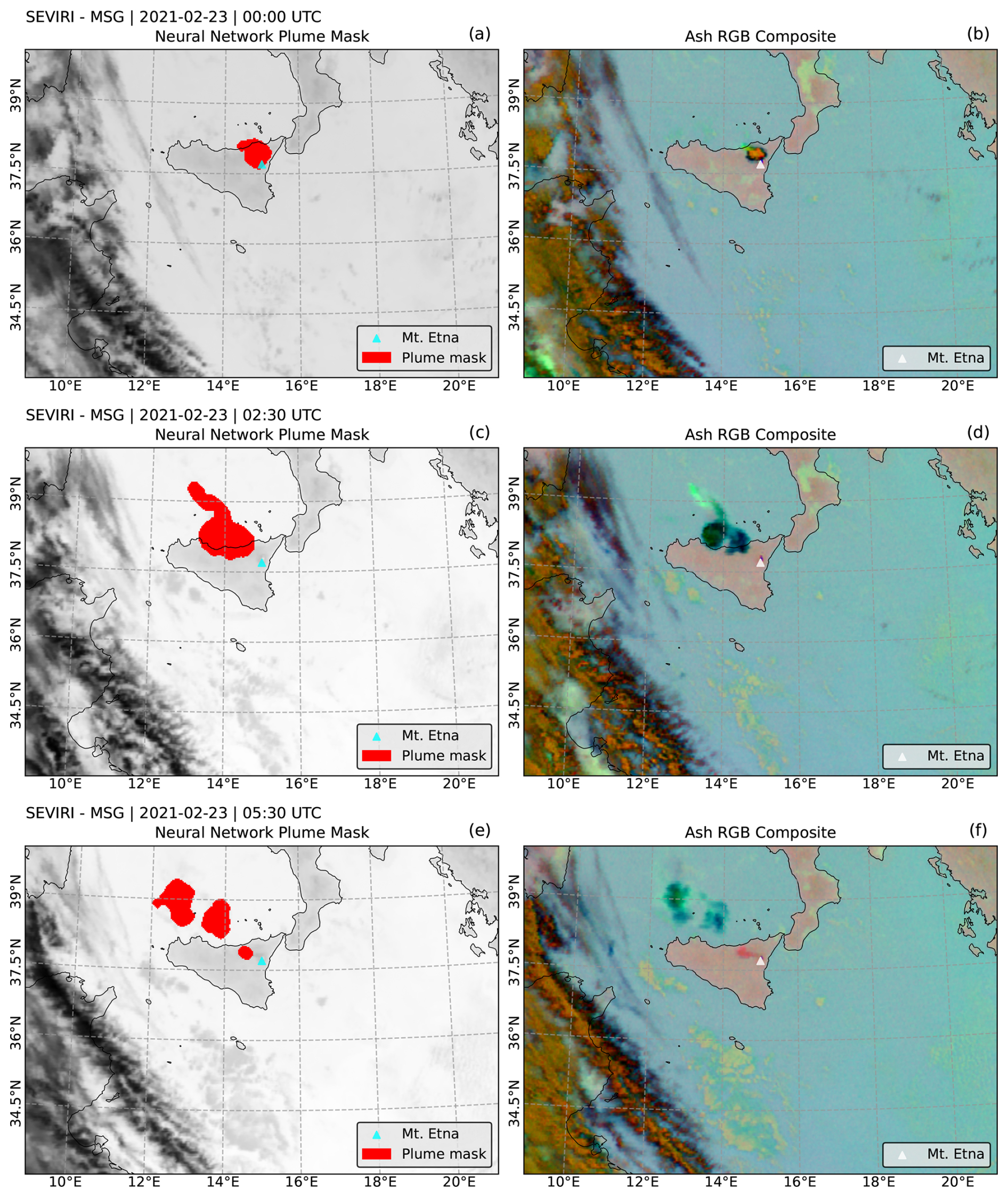
Figure 5 Sequence of SEVIRI images showing the evolution of the volcanic cloud from 22–23 February 2021. The left panel shows the plume mask (in red) generated by the filtered NN model, overlaid on the brightness temperature at 10.8 µm. The right panel shows the standard Ash RGB composite. In all images, Mount Etna's location is marked with a white triangle. (a, b) correspond to 00:00 UTC, (c, d) to 02:30 UTC, and (e, f) to 05:30 UTC. The full image sequence is provided in the Supplements (Video 1).

Unfortunately, in the presented version of the post-processing algorithm, not all “noisy” pixels can be effectively removed through the application of the NL means filter. In addition, the tracking algorithm does not include a control to prevent excessive growth of the circular region, which may become problematic during near-real-time operations when tracking volcanic clouds over long time periods. Under such circumstances, a more sophisticated post-processing algorithm could be developed. An example of a real image before and after the application of this processing step is presented in Fig. 2f. The algorithm is also robust in tracking fragmented volcanic clouds, as shown in Fig. 5e in the Results section.

Finally, the results and evaluation metrics presented in the Results section correspond to the filtered plume masks obtained after the application of this post-processing step.

3.5 Evaluation metrics

The performance of the binary classification between the VC and NVC classes was evaluated using a set of standard metrics, which are briefly defined in this section (Fawcett, 2006; Rainio et al., 2024). In this study, the convention adopted is as follows: the outcome of the manual labelling process is defined as the observed data, whereas the outcome of the classification process produced by the NN model is defined as the predicted data. Both observed and predicted data are considered positive when they belong to the VC class, and negative when they belong to the NVC class. Thus, considering this convention, each pixel prediction can be classified into one of four possible categories:

• True Positive (TP): The observed class is VC, and the predicted class is also VC. Therefore, the VC class is correctly predicted.

• False Positive (FP): The observed class is NVC, whereas the predicted class is VC. In this case, the VC class is incorrectly predicted.

• False Negative (FN): The observed class is VC, whereas the predicted class is NVC. In this case, the NVC class is incorrectly predicted.

• True Negative (TN): The observed class is NVC, and the predicted class is also NVC. Therefore, the NVC class is correctly predicted.

The total number of predictions in each category can be represented in a 2 × 2 matrix, known as the confusion matrix (C), which provides a visual representation of the classification results. In this matrix, TP is located at C_0,0, FP at C_0,1, FN at C_1,0, and TN at C_1,1.

Based on the confusion matrix, several standard metrics for binary classification can be calculated. These metrics include accuracy, balanced accuracy, precision, recall, and F1-score, all of which range from 0 (poor performance) to 1 (optimal performance).

• Accuracy: The proportion of correctly predicted pixels divided by the total number of pixels.

  $$\begin{array}{}\text{(1)}& \text{Accuracy}={\displaystyle \frac{\mathrm{TP}+\mathrm{TN}}{\mathrm{TP}+\mathrm{FP}+\mathrm{FN}+\mathrm{TN}}}\end{array}$$

• Balanced accuracy: A metric that measures the prediction performance for each class (VC and NVC) independently and then computes their average (Velez et al., 2007). This metric is particularly appropriate for the evaluation of imbalanced datasets.

  $$\begin{array}{}\text{(2)}& \text{Balanced\hspace{0.17em}\hspace{0.17em}Accuracy}={\displaystyle \frac{\frac{\mathrm{TP}}{\mathrm{TP}+\mathrm{FN}}+\frac{\mathrm{TN}}{\mathrm{TN}+\mathrm{FP}}}{\mathrm{2}}}\end{array}$$

• Precision: The proportion of TP predictions divided by the total number of pixels predicted as VC.

  $$\begin{array}{}\text{(3)}& \text{Precision}={\displaystyle \frac{\mathrm{TP}}{\mathrm{TP}+\mathrm{FP}}}\end{array}$$

• Recall: The proportion of TP predictions divided by the total number of pixels observed as VC.

  $$\begin{array}{}\text{(4)}& \text{Recall}={\displaystyle \frac{\mathrm{TP}}{\mathrm{TP}+\mathrm{FN}}}\end{array}$$

• F1-score: The harmonic mean of precision and recall, providing a single metric that combines both measures.

  $$\begin{array}{}\text{(5)}& \text{F1}={\displaystyle \frac{\mathrm{2}\cdot \text{Recall}\cdot \text{Precision}}{\text{Precision}+\text{Recall}}}\end{array}$$

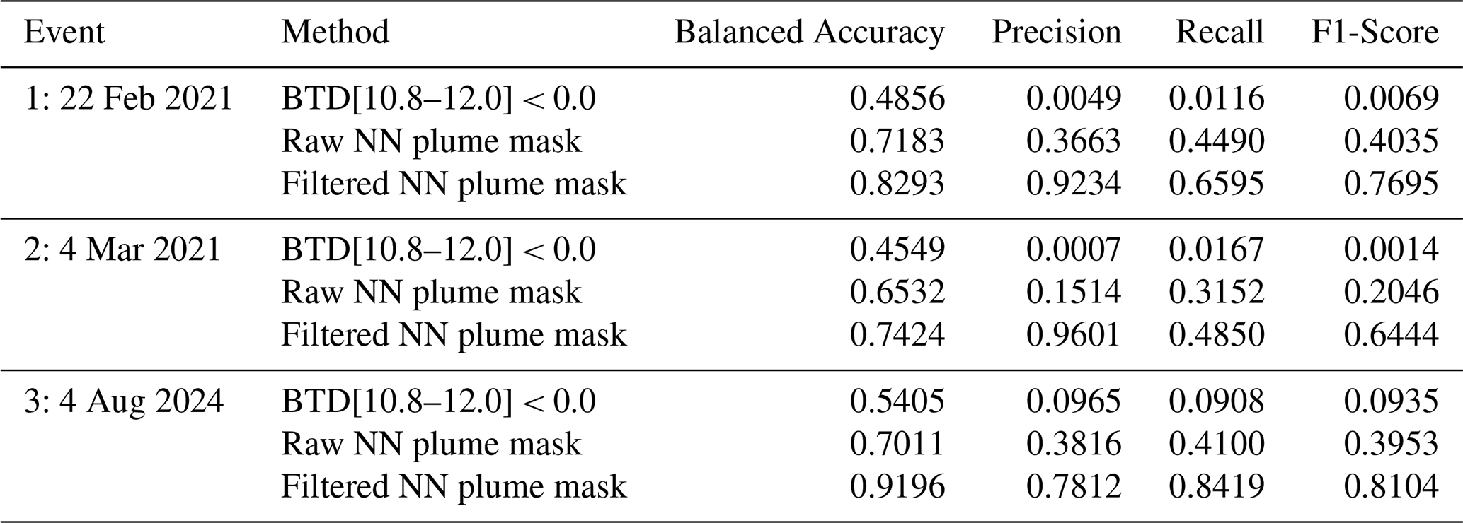
Table 5 Overall performance metrics for the complete image sequences of the three validation events obtained using the filtered NN plume mask. Metrics derived from the BTD method and the raw NN plume mask are also presented for comparison.

It is worth noting that the accuracy metric was used for the training and testing datasets, whereas balanced accuracy was used for the validation dataset. This choice was made because the validation dataset is highly imbalanced, making balanced accuracy metric more appropriate for this type of dataset.

3.6 Retrieval comparison

An additional analysis was conducted to estimate the volcanic cloud mass loading from both the manually observed data and the NN predicted data. The mass loading was retrieved using the Volcanic Plume Removal (VPR) algorithm (Pugnaghi et al., 2013, 2016), where the pixels classified by the NN model as VC class were used as input to the retrieval procedure.

Since the NN model output generates a general plume mask containing ash, ice, and SO₂ without discriminating among these components, the procedure adopted to apply the VPR algorithm separately to each component was the same as that presented in Guerrieri et al. (2023). In this procedure, Radiative Transfer Model (RTM) computations were performed to derive a BTD[10.8–12.0] threshold. Accordingly, a positive BTD[10.8–12.0] threshold was used to discriminate ash from ice within the NN predicted plume mask, whereas the SO₂ retrieval was applied to the entire plume mask. The thresholds used for each event were 1.15 for Event 1, 1.12 for Event 2, and 1.25 for Event 3. For further details regarding the calculation of the BTD[10.8–12.0] thresholds, see Sects. 2.2 and 2.3 in Guerrieri et al. (2023).

The retrievals derived from the NN predicted plume masks were subsequently compared with those obtained from the manually generated plume masks (using the same BTD[10.8–12.0] thresholds).

3.7 Explainability method

As outlined in the Sect. 3.2, the NN model consists of three hidden layers with 60 neurons each one and uses 13 input features, resulting in a complex model. This level of complexity limits the understandability of the model's classification process (Flora et al., 2024). In order to better understand the classification process, an explainability method called Shapley Additive Explanations (SHAP) was used. SHAP values is a game theoretic framework that quantifies the contribution of each feature to individual predictions, thereby providing insight into the model's overall internal mechanisms (Lundberg et al., 2017).

The discussion section presents a beeswarm plot illustrating feature relevance for the NN model based on the testing set. The beeswarm plot displays the features along the y axis, ordered according to their influence on the model prediction, from the highest to the lowest. The impact of each feature on the prediction is represented along the x axis through the SHAP values, while each dot corresponds to a pixel from the testing dataset. Positive SHAP values indicate a positive contribution to the prediction of the VC class, whereas negative SHAP values indicate a contribution toward the prediction of the NVC class. The color of the dots indicates whether the corresponding pixel exhibits a high or low value for the respective feature.

4 Results

This section presents the detection results obtained for the three validation events listed in Table 4. The results are summarized in Table 5, which reports the performance metrics derived from the filtered NN plume mask, together with those obtained from the raw NN plume mask and the BTD method for comparison.

It is worth noting that all results presented in this section were obtained using a calibrated probability threshold of 0.8 for the classification of VC pixels, as described in Sect. 3.2 and illustrated in Fig. 3.

The metrics reveal that the overall balanced accuracy for all validation events reached values between 74.2 % and 92.0 % when using the filtered NN plume mask, whereas the raw NN plume mask achieved values up to 71.8 %. In contrast, the BTD method reached a maximum balanced accuracy of 54.0 %. The balanced accuracy was used for the validation dataset because the classes are highly imbalanced, and the standard accuracy (Eq. 1) may lead to misleading interpretations of the results. Along with the balanced accuracy shown in Table 5, the precision, recall, and F1-score metrics are also presented. Due to the importance of detecting volcanic clouds and the risks they pose to aviation safety, special attention was given to the precision and recall metrics.

In general, considering all metrics presented in Table 5, the filtered NN plume masks showed the best performance across all validation events.

4.1 Event 1: 22–23 February 2021

This event was a paroxysmal episode at the Southeast Crater, which lasted 10 h. It was primarily characterized by a lava fountain with a duration of 50 min and a volcanic cloud that reached more than 11 km in height (Guerrieri et al., 2023; INGV, 2021b).

At the onset of this event, the volcanic cloud was dispersed toward the northwest, and it is observed with a thick core displaying brown shades, indicating a high concentration of particles, presumably ash. In contrast, the cloud's edges appear in dark blue tones, suggesting thinner regions primarily composed of ice (see Fig. 5b). As the eruption progresses, the denser portion of the cloud disperses and eventually appears entirely dark blue, highlighting a strong presence of ice. Additionally, a sulphur dioxide (SO₂) signal is visible in the northern part of the cloud, represented in green tones (see Fig. 5d). By the end of the sequence, the primary volcanic cloud has dissipated, and a new eruptive pulse produces a low-level volcanic cloud, visible in red shades in Fig. 5f.

Notably, in Fig. 5a, c, and e, the NN model effectively detects most components and the overall structure of the volcanic cloud throughout its evolution, even when the cloud becomes fragmented as is revealed in Fig. 5e. The balanced accuracy for the complete image sequence of this event was 82.9 %, while the precision, recall, and F1-score were 92.3 %, 66.0 %, and 77.0 %, respectively, as reported in Table 5.

The time series of the precision and recall metrics for each image in the sequence using the filtered NN plume mask are presented in Fig. 8a. It can be observed that both precision and recall are high at the beginning of the eruption, with values between 80 % and 90 %, but decrease to below 80 % during the middle stage of the eruption.

4.2 Event 2: 4 March 2021

This second event was produced by a strombolian activity at the Southeast Crater, which started at 07:50 UTC. The activity then evolved into a lava fountain that generated a volcanic cloud rising to more than 11 km (Guerrieri et al., 2023; INGV, 2021a).

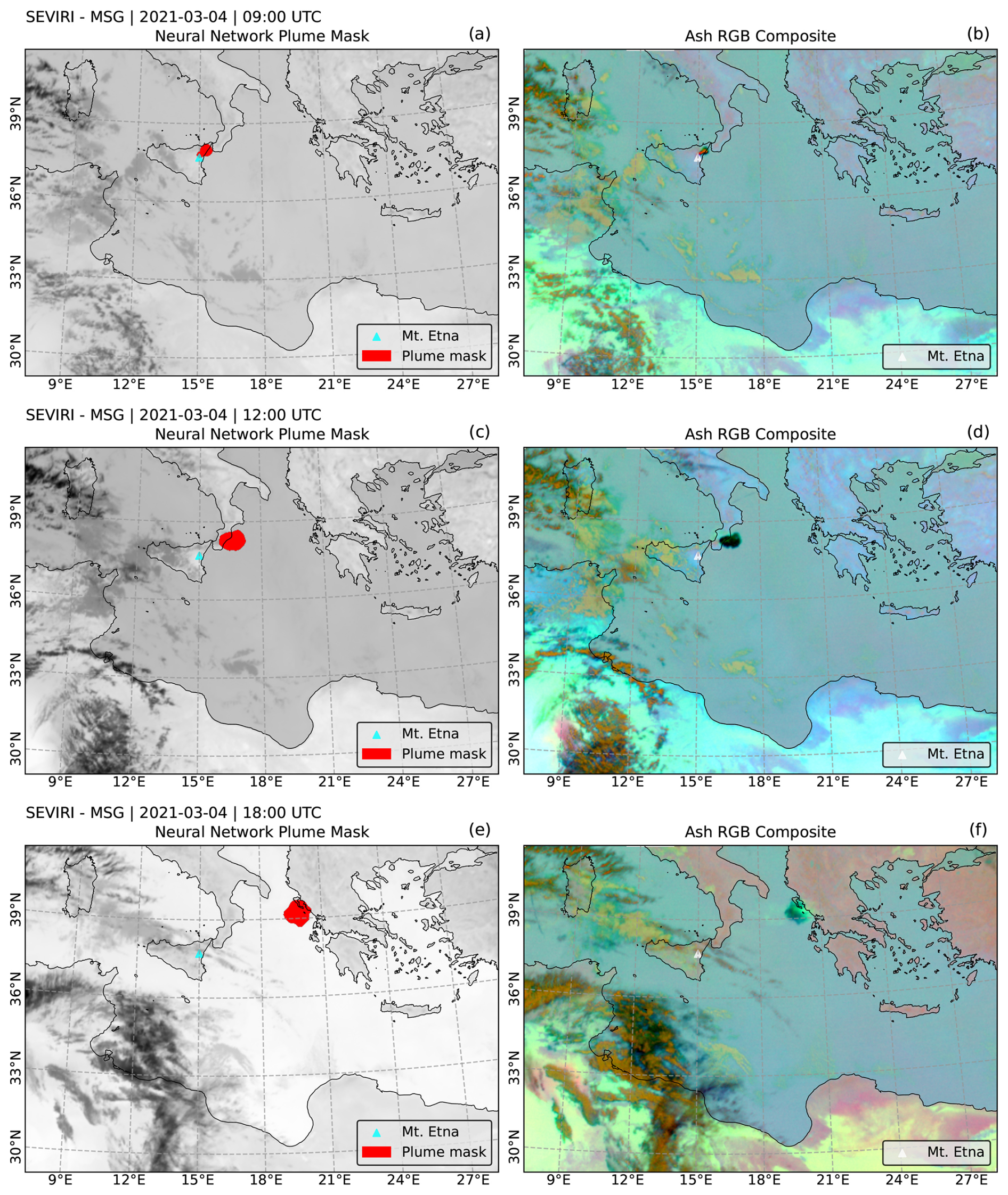
Figure 6 Sequence of SEVIRI images showing the evolution of the volcanic cloud from 4 March 2021. The left panel shows the plume mask (in red) generated by the filtered NN model, overlaid on the brightness temperature at 10.8 µm. The right panel shows the standard Ash RGB composite. In all images, Mount Etna's location is marked with a white triangle. (a, b) correspond to 09:00 UTC, (c, d) to 12:00 UTC, and (e, f) to 18:00 UTC. The full image sequence is provided in the Supplement (Video 2).

For this event, the composition of the volcanic cloud is quite similar to the previous case. In this instance, the cloud moves toward the northeast. At the onset, ash particles are observed in the inner part of the cloud, shown in brown shades (see Fig. 6b), which are later masked by ice (see Fig. 6d). Additionally, the SO₂ signal, visible in green, becomes more prominent toward the end of the sequence.

Unlike the previous case, this volcanic cloud remains compact, and the NN model successfully detects most parts of the cloud throughout the sequence (see Fig. 6a, c, and e). The cloud was continuously tracked for 12 h and over a distance exceeding 550 km from the volcano. Toward the end of the sequence, some portions of the volcanic cloud containing SO₂ are no longer detected, as illustrated in Fig. 6f. The reduced detection performance is likely attributable to cloud dilution in those areas, resulting in an overall balanced accuracy for the complete image sequence of 74.2 %, a precision of 96.0 %, but lower recall and F1-score values of 48.5 % and 64.4 %, respectively, as reported in Table 5.

Figure 8b shows the evolution of the precision and recall metrics for each image in the sequence. It is worth noting that, at the beginning of the eruption, this event presented the highest recall values among the three validation events, with values close to 100 %. In other words, during the initial stage of the eruption, the filtered NN plume mask detected nearly all pixels observed as VC. However, the recall metric decreased around 11:00 UTC, corresponding to the moment when the volcanic cloud passed over the continental surface, before increasing again and subsequently decreasing to below 80 % during the middle stage of the sequence.

4.3 Event 3: 4 August 2024

This last validation event was also produced by a lava fountain, this time from the Voragine Crater, starting at 03:20 UTC. The fountain generated a volcanic cloud that rose to over 10 km (INGV, 2024). The volcanic cloud exhibited wind-driven behaviour, dispersing toward the east and southeast. This case is particularly challenging, as the volcanic cloud is composed of ash, ice, and SO₂, and is both surrounded and mixed with meteorological clouds.

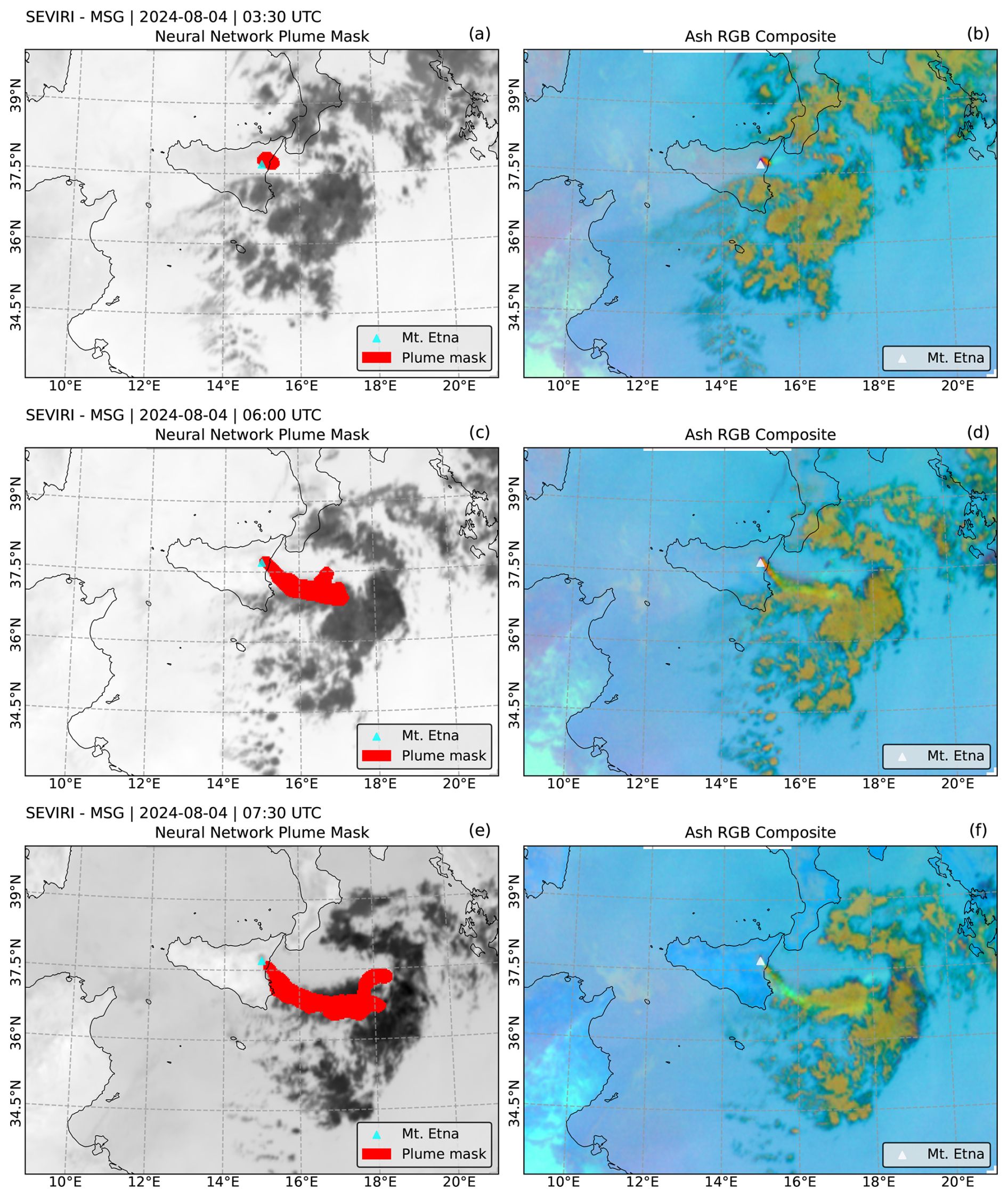
Figure 7 Sequence of SEVIRI images showing the evolution of the volcanic cloud from 4 Agust 2024. The left panel shows the plume mask (in red) generated by the filtered NN model, overlaid on the brightness temperature at 10.8 µm. The right panel shows the standard Ash RGB composite. In all images, Mount Etna's location is marked with a white triangle. (a, b) correspond to 03:30 UTC, (c, d) to 06:00 UTC, and (e, f) to 07:30 UTC. The full image sequence is provided in the Supplement (Video 3).

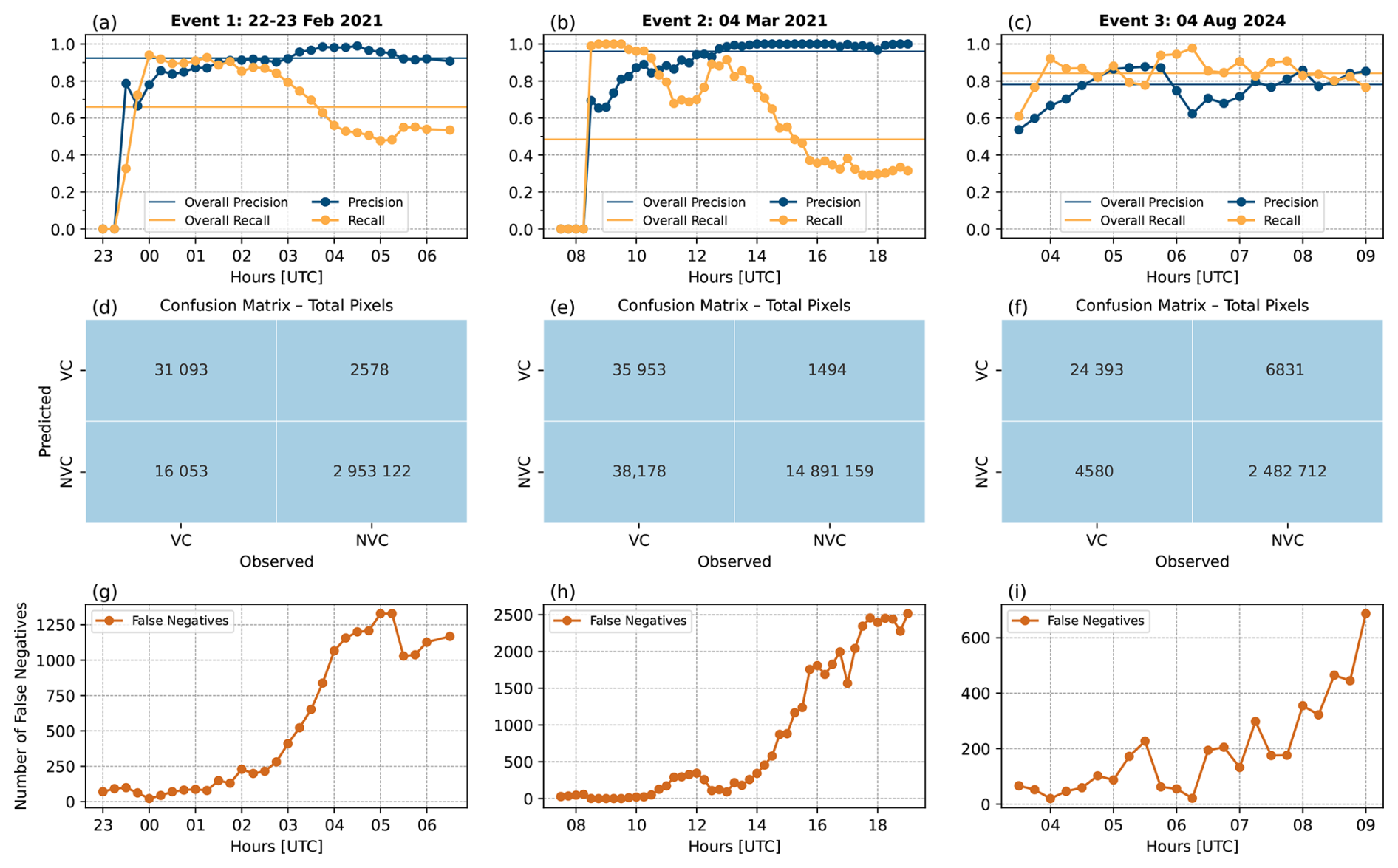
Figure 8 Precision and recall metrics, confusion matrices and false negatives number evolution for the validation events using the filtered NN plume mask. (a), (d) and (g) show the evolution of metrics, the confusion matrix and false negatives number evolution for the Event 1. (b), (e) and (h) the same as the previous but for Event 2. (c), (f) and (i) the same as the previous one but for Event 3.

At the onset, the volcanic cloud appears in red shades, with some SO₂ signal in green (see Fig. 7b), before encountering the mid-level meteorological clouds. Note how the volcanic and meteorological clouds blend in Fig. 7d and f. Detecting volcanic clouds under these conditions is generally very difficult as reported in previous studies (Prata et al., 2022; Taylor et al., 2023). Nevertheless, the filtered NN plume mask successfully identified the volcanic cloud, and the tracking algorithm subsequently followed its evolution even when it was blended with meteorological clouds (see Fig. 7a, c, and e). For this event, the overall balanced accuracy obtained was 92.0 %, while the other performance metrics were 78.1 % precision, 84.2 % recall, and 81.0 % F1-score, as reported in Table 5. The evolution of the precision and recall metrics across the image sequence is shown in Fig. 8c. It can be observed that these metrics remain above 80 % for recall and above 60 % for precision during most of the sequence.

4.4 Metrics analysis

As can be seen in Table 5 and the Fig. 8a–c, the metrics indicate strong performance across all validation events using the filtered NN plume mask. Looking at the precision and recall metrics, we can gain deeper insight into the performance of the filtered NN plume mask. For instance, the precision values for Event 1 and Event 2 are 92.3 % and 96.0 %, respectively, indicating that 92.3 % and 96.0 % of the pixels detected as VC in each event were correctly classified. These high precision values indicate that the detection was highly reliable, with only 7.7 % and 4.0 % of the detected pixels corresponding to false alarms, respectively.

Whereas the recall values for Event 1 and Event 2 are 66.0 % and 48.5 %, respectively, indicating that the model was able to detect 66.0 % and 48.5 % of the VC pixels observed in the reference plume mask. In other words, the filtered NN plume mask failed to detect 34.0 % and 51.5 % of the VC pixels observed in the reference plume mask for Event 1 and Event 2, respectively.

These relatively low recall values are likely due to dilution in the outer portions of the volcanic cloud, which fall below the detection limit of our NN model, although they remain visible to a human operator in the images. This hypothesis was also proposed by Theys et al. (2013). The limitation in detecting the more dilute portions of the volcanic cloud was previously discussed in Sect. 4.1 and 4.2, where the effect became evident toward the end of the sequence. This is expected, as dilution increases over time as the cloud disperses, resulting in more false negatives for the NN model.

The low overall recall values for the complete image sequence in Event 1 and Event 2 contrast with the recall values obtained for the individual images within the sequence, as shown in Fig. 8a–c, where high recall values are observed during the early stages of the volcanic clouds.

On the other hand, for Event 3, the behaviour of the precision and recall metrics is opposite to that observed in the previous events. In this case, the precision is lower at 78.1 %, while the recall is significantly higher at 84.2 %. In other words, the recall indicates that in Event 3, the filtered NN plume mask missed only 15.8 % of the VC pixels observed in the reference plume mask. Furthermore, the precision reveals that 78.1 % of the pixels detected as VC were correctly identified, indicating that 21.9 % of the detected pixels were false alarms.

These results may be attributed to the challenging nature of Event 3, in which the volcanic cloud is mixed with and surrounded by meteorological clouds. Under these circumstances, the human operator responsible for generating the manual plume mask may have faced difficulty in identifying the volcanic cloud and distinguishing it from meteorological clouds. Despite this complexity, the NN model successfully detected the volcanic cloud throughout the sequence (see the Video 3 in the Supplement).

The issue of the false negatives, likely caused by the dilution of the volcanic cloud is evident when examining the confusion matrices for the complete images sequence for each event, shown in Fig. 8d–f. These confusion matrices are constructed using the predictions (detections) of the filtered NN plume mask and the observed (reference) plume mask (Fawcett, 2006). In Fig. 8d–f the predictions are on the y axis and the observations on the x axis.

As previously discussed, the effect is more pronounced in the Event 1 and Event 2, which reach overall false negatives of 16 000 and 38 000 pixels, respectively, for the complete sequence. Meanwhile, for Event 3 the false negatives are 4500 pixels. It is important to note that Events 1 and 3 have similar durations, lasting approximately 6 h, whereas Event 2 lasted approximately 12 h. As a result, the total number of SEVIRI images analysed varied among the three events.

The question arises as to how the most challenging event achieved lower false negatives. We suggest that the answer lies in the generation of the manual plume mask. When the volcanic cloud is difficult to distinguish from meteorological clouds, the reference plume mask tends to be smaller and may not extend to the more dilute portions of the cloud. This situation reveals not only the potential of the NN model but also the limitations of the human operator under challenging conditions.

Furthermore, as illustrated in Fig. 8g–i, the number of false negatives progressively increases over time, as expected under the hypothesis that the dilution of the volcanic cloud leads to an increase in false negatives predictions. Consequently, lower recall values are obtained. This behaviour can be observed comparing Fig. 8a–c and g–i, where an increase in the number of false negatives corresponds to a decrease in the recall metrics.

Full animations illustrating the model's performance over the complete sequence are provided in the Supplement, including one animation for each validation event. These animations allow spatial visualization of true positives, false negatives, and false positives.

5 Discussion

The aim of this work was to explore the detection of volcanic clouds containing a mixture of ash, ice, and SO₂, with a focus on leveraging machine learning techniques and data from the SEVIRI sensor. The results presented in the previous section demonstrate that the filtered neural network model is capable of detecting volcanic clouds under challenging conditions, achieving high performance metrics, as shown in Table 5 and Fig. 8a–c. These findings contrast with previous studies (Gupta et al., 2022; Prata et al., 2020; Rose et al., 1995; Taylor et al., 2023), where traditional methods (i.e. a negative BTD[11–12]) cannot be used to detect volcanic clouds in the presence of ice or water droplets. Therefore, our results provide compelling evidence that machine learning techniques enable the detection of volcanic clouds even in challenging scenarios.

To assess the impact of false negatives in the NN model predictions, an additional analysis was conducted to estimate the volcanic cloud mass loading using the filtered NN plume mask and to compare it with the mass loading obtained from the manually generated plume masks reported in Guerrieri et al. (2023) (see Sect. 3.6 for further details).

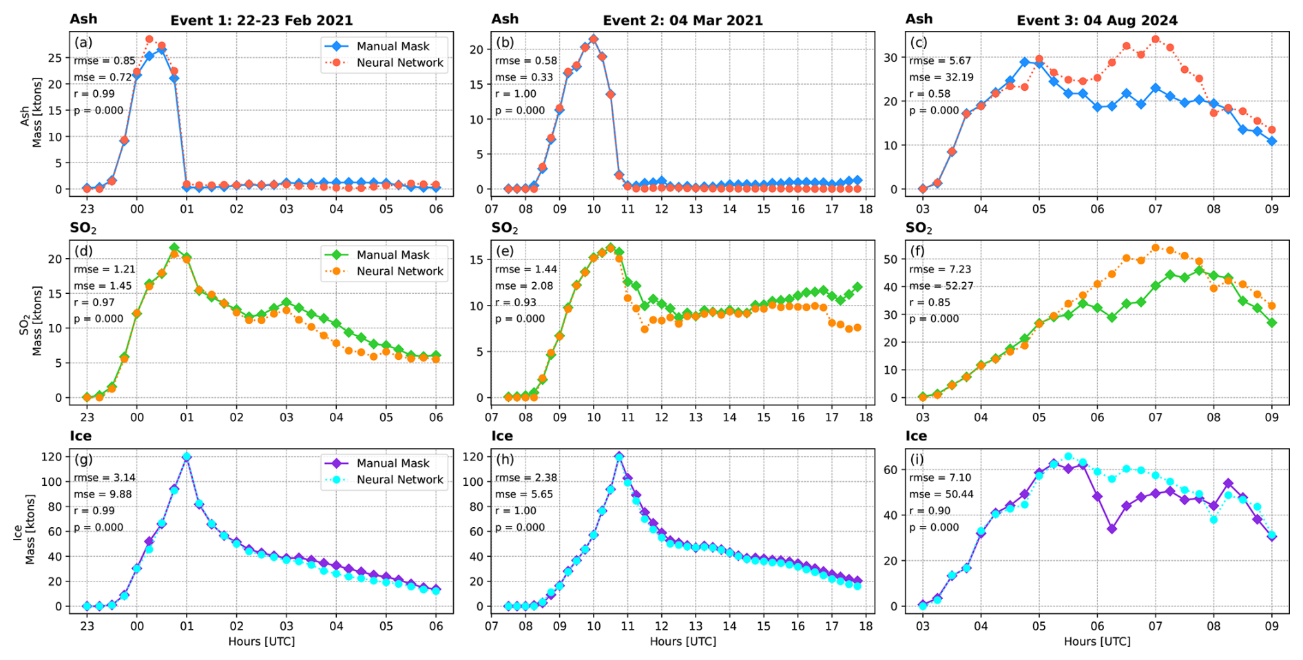
Figure 9 Comparison of mass loading derived from the filtered NN plume mask and the manual plume mask. The left panel shows the mass loading evolution of ash, SO₂, and ice for Event 1 (22–23 February 2021). The central panel presents the same analysis for Event 2 (4 March 2021), and the right panel for Event 3 (4 August 2024). Error and correlation metrics between the two estimations are also reported.

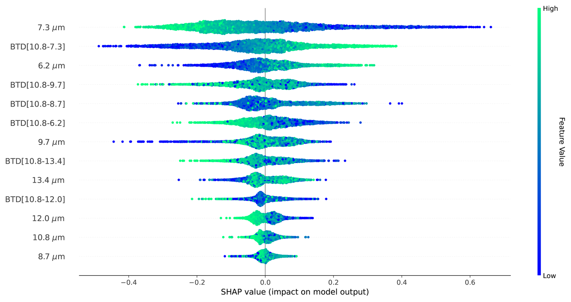
Figure 10 Feature relevance plot for the 13 features present in the volcanic cloud detection dataset. Scatter points are SHAP values, while the color coding indicates the minimum-maximum normalized value for each feature.

The comparison is presented in Fig. 9, where the left panel shows the comparison of mass loading of ash, SO₂, and ice for Event 1, the central panel for Event 2, and the right panel for Event 3.

As can be seen in Fig. 9, the evolution of ash, SO₂, and ice mass loading derived from the filtered NN detection is in exceptionally good agreement with that obtained from the manually generated plume masks. Note that, in all retrievals presented in Fig. 9, the largest differences occur in the middle or final stages of the sequence, coinciding with an increase in the false negatives (see Fig. 8g–i). Nevertheless, the influence of false negatives on the mass loading estimation appears to be minimal, as indicated by the generally strong correlation and low error values. Event 3 again exhibits the largest differences, likely due to its challenging nature and the difficulty faced by the human operator in discriminating the volcanic cloud from meteorological clouds during the generation of the plume masks. The quantitative comparison supports the hypothesis that the pixels missed by the NN model correspond to the most diluted portions of the volcanic cloud, which apparently do not contribute significantly to the overall mass loading estimation.

A further point of discussion concerns the interpretation of the detections produced by the NN model through the use of SHAP values, as introduced in Sect. 3.7.

The performance achieved by the NN model in the validation events is likely attributable to the integration of all 13 input features, including the full set of thermal-infrared channels (6–14 µm), and the ability of machine learning models to exploit multiple inputs to learn relevant multivariate relationships. Thus, to provide insight into the NN model's internal mechanisms, Fig. 10 presents the feature relevance ranked according to their mean absolute SHAP values.

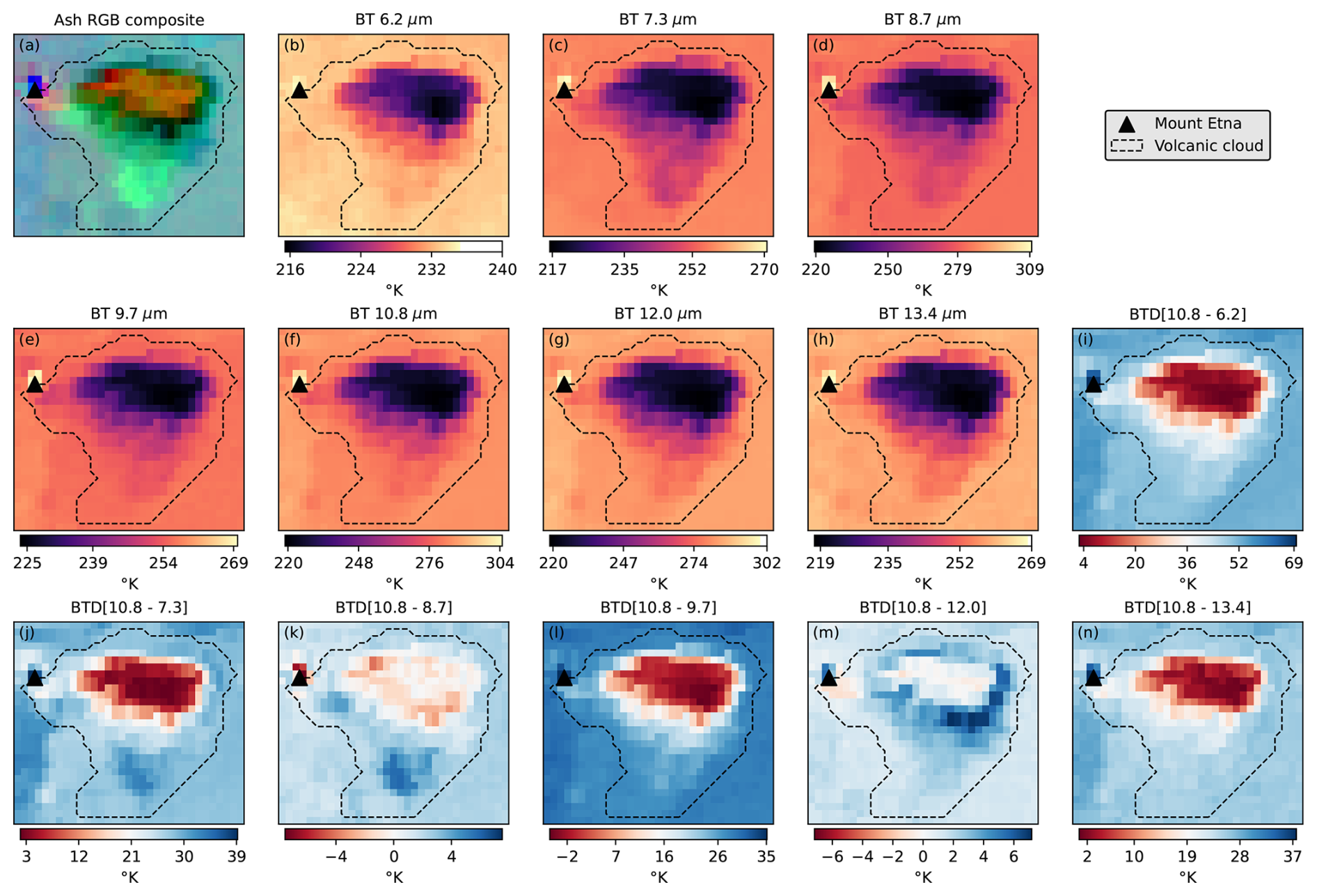
Figure 11 Zoom in on the volcanic cloud from 19 February 2021, as shown in Fig. 1. Panel (a) displays the Ash RGB composite (same as Fig. 1b), while panels (b)–(n) present all the features used during model training phase. Also shown is an overlaid hand-drawn volcanic cloud boundary, created during the labelling process.

According to Fig. 10, it is interesting to note that the most relevant feature is the brightness temperature at 7.3 µm channel, followed by the BTD[10.8–7.3], and then the 6.2 µm channel. The 7.3 and 6.2 µm channels are known as the lower-level water vapour and the upper-level water vapour, respectively. Also, they are used to identify and track atmospheric elements (Schmit and Gunshor, 2020). The high relevance attributed to the 7.3 µm channel is likely related to the strong SO₂ absorption occurring at this wavelength (Pavolonis et al., 2020), as well as to the cold and optically thick characteristics of some volcanic clouds analysed in this study, which are effectively detected by the 7.3 µm channel. In addition, this channel provides good discrimination between volcanic clouds and clear land or sea surfaces (see Fig. 11c).

Following in the feature relevance ranking, BTD[10.8–9.7] and BTD[10.8–8.7] appear in fourth and fifth place, respectively. The BTD[10.8–8.7] feature is commonly used for the detection of semi-transparent ice clouds (Wang et al., 2011) and appears as an important feature here because of the presence of ice in some of the volcanic clouds analysed in this study.

The BTD[10.8–12.0], widely recognized as the standard method for volcanic cloud detection ranks tenth, being surpassed even by the 13.3 µm channel. This result is expected, since negative BTD[10.8–12.0] values are more sensitive to semi-transparent ash-rich volcanic clouds, whereas the volcanic clouds considered in the present study were predominantly opaque and rich in ice and SO₂.

The SHAP value distributions for each feature in Fig. 10 also help to explain how the model operates. For instance, at the 7.3 µm channel, the SHAP values indicate that lower temperatures contribute positively to the prediction of the VC class, whereas higher temperatures, at the 7.3 µm channel, are associated with negative SHAP values, indicating a negative contribution to the VC class prediction and therefore favouring the NVC class. This behaviour is expected because, in the presence of SO₂, the 7.3 µm channel is affected by absorption. Similarly, cold or optically thick volcanic clouds produce lower brightness temperature values in this channel. Another interesting example is provided by the BTD[10.8–12.0] feature. Low BTD[10.8–12.0] values, represented by blue tones, are generally associated with positive SHAP values, indicating a positive contribution to the prediction of the VC class. In contrast, high BTD[10.8–12.0] values are associated with negative SHAP values, indicating a contribution toward the prediction of the NVC class.

To complement the results provided by the SHAP values in Fig. 10, Fig. 11 displays a zoom in on the volcanic cloud from 19 February 2021, as shown in Fig. 1. Panel (a) displays the Ash RGB composite (same as Fig. 1b), while panels (b) through (n) present all the features. The information presented in Fig. 7b–n, together with the feature relevance shown in Fig. 10, provides insight into the relationships learned by the NN model.

The behavior of the 7.3 µm channel, as indicated by the SHAP values, is confirmed in Fig. 11c, where lower brightness temperature values at the 7.3 µm channel are shown to align closely with the spatial extent of the volcanic cloud. Indeed, among all the features, the 7.3 µm channel most effectively represents the volcanic cloud in that case.

The limitation of the BTD[10.8–12.0] is evident in Fig. 11m, where the volcanic cloud exhibits BTD[10.8–12.0] values close to or higher than 0.0. As previously discussed, this behaviour is expected due to the optically thick characteristics of the volcanic cloud, together with the presence of ice, both of which can reduce the effectiveness of this method for volcanic cloud detection.

6 Conclusions

We presented a neural network model to detect volcanic clouds containing a mixture of ash, ice, and SO₂ using data from the SEVIRI sensor onboard the geostationary satellite Meteosat-10 and -11. This study also described the generation of a training dataset, based on manual plume masks from more than 1200 SEVIRI images. The result was a balanced binary training dataset comprising more than 2 200 000 pixels, with 13 features corresponding to seven thermal infrared bands and six BTDs. Furthermore, a tracking algorithm was proposed to improve the performance of the NN model. The volcanic cloud detection produced by the filtered NN plume mask achieved a balanced accuracy of 92.0 %, whereas the raw NN plume mask achieved only 71.8 %, demonstrating the effectiveness of the tracking algorithm applied during the post-processing step. Using the filtered NN plume mask, the results showed that the model successfully detected 66.0 %, 48.5 %, and 84.1 % of the observed volcanic cloud pixels in the three analysed validation events, respectively. In addition, only 7.7 %, 4.0 % and 21.9 % of the detected volcanic cloud pixels corresponded to false alarms for the respective events.

The integration of the NN model with the proposed plume tracking method enabled the tracking of the volcanic cloud across the image sequences for up to 12 h. This strong performance demonstrates the ability of machine learning models to leverage multiple input features and learn complex multivariate relationships to address challenging detection problems, such as volcanic clouds in complex scenarios involving mixtures of ash, ice, and SO₂. In summary, this work shows that it is possible to automatically detect volcanic clouds in such complex scenarios.

However, the NN model shows limitations in detecting more diluted portions of the volcanic clouds, likely due to insufficient representation of such cases in the training dataset or because the signal falls below the sensor's detection limit. This limitation becomes evident when analysing the false negative evolution, which increases during the middle and final parts of the image sequences for the three analysed Mount Etna eruption case studies of 22 February 2021, 4 March 2021 and 4 August 2024.

Nevertheless, we demonstrated that the false negatives generated by the dilution process do not significantly affect the mass loading estimation. However, the inability to detect these diluted portions may have implications for aviation safety. Future work should focus on this limitation to determinate whether reliable detection of diluted cloud regions is feasible.

Overall, the results are encouraging and provide valuable insight into the development of a near-real-time and automatic detection system for volcanic clouds, which is highly desirable for aviation safety and could be useful for the VAACs that deal routinely with volcanic clouds rich with ice and SO₂.

An important question for future studies is to determine whether it is feasible to apply transfer learning using the same NN model to extend its application to new generations of geostationary sensors (e.g. Meteosat-12 FCI, Himawari AHI, and GOES ABI) and to additional eruption case studies worldwide. Addressing this question would require experiments to evaluate the performance of the NN model using data acquired from different sensors and volcanic eruptions occurring at different geographical locations. This approach could eventually lead to the training of a new NN model based on the same architecture adopted in this work, but using representative datasets derived from the new case studies and satellite sensors.

Appendix A: Description of the events included in the balanced dataset

Table A1 presents a brief description of the volcanic cloud composition observed during each eruptive event, together with the list of SEVIRI image sequences used to generate the balanced dataset. The description of the volcanic cloud is based on the color interpretation provided in the SEVIRI Ash RGB Quick Guide (Ash RGB Quick Guide | EUMETSAT – User Portal, 2025).

Table A1 Description of the eruptive events and corresponding SEVIRI image sequences used to generate the balanced dataset.