Cloud fields and aerosol classification with lidar using advanced AI approach

Understanding the vertical distribution of aerosol and clouds i.s critical for climate modeling, weather forecasting, and air quality monitoring. Lidar observations are central to profiling atmospheric composition, yet signal attenuation in optically thick layers limits the effective retrieval of some important properties above those layers. More complex measurement approaches, using a combination of Lidar and cloud radar systems, can be taken to support more inclusive and accurate inference. In this study, we develop a deep learning framework to address this trade-off and gap in the cost of data acquisition by enabling full-column aerosol and cloud classification using only standard lidar inputs, achieving particularly high skill for aerosol typing while demonstrating robust, physically consistent classification of ice-cloud fields even under conditions of strong lidar signal attenuation, with liquid-cloud uncertainties primarily arising from closely related microphysical classes. The approach is based on a U-Net architecture trained to predict combined aerosol and cloud types from vertical profiles of backscatter and depolarization. Classification targets integrate established aerosol typing from PollyXT with cloud and precipitation categorization from Cloudnet, facilitating a unified scheme. The model achieves high precision, recall, and F1-scores above 95 %. By evaluating numerous complex case studies, we establish the model's ability to exploit information embedded in the lidar signal below attenuating layers, including structural and contextual features, to infer atmospheric conditions at higher altitudes, offering a robust AI-based enhancement to lidar-based atmospheric profiling and target classification. The application of AI in this context closes the gap between the need for vertical cloud maps and the sparse availability of Cloudnet.

1 Introduction

Aerosols and clouds are fundamental components of the Earth's atmosphere, exerting profound influences on the planet's climate system. They modulate radiative energy balance through scattering and absorption of solar and terrestrial radiation, significantly impacting the hydrological cycle through precipitation processes (Ramanathan et al., 2001; Albrecht, 1989). They also play a role in atmospheric chemistry by interacting with gases and providing surfaces for chemical reactions to occur (Intergovernmental Panel on Climate Change (IPCC), 2014; Jacob, 2000; Lelieveld and Crutzen, 1991). Clouds, in particular, have large but opposing effects on short-wave and long-wave radiation, resulting in a significant net cooling effect globally, although the magnitude remains uncertain (Hartmann and Doelling, 1991). Aerosol-cloud interactions (ACI) represent one of the largest uncertainties in current climate projections (Intergovernmental Panel on Climate Change (IPCC), 2014; Rosenfeld et al., 2014). Understanding the vertical distribution and properties of both aerosol and clouds is therefore critical to accurately understand and quantify their climatic impacts and to improve the representation of atmospheric processes in weather prediction and climate models (Winker et al., 2010; Weitkamp, 2005; Rogozovsky et al., 2023).

Significant progress has been made in the development of remote sensing techniques capable of profiling atmospheric constituents. Lidar has emerged as a powerful tool for providing detailed vertical profiles of aerosol particles and clouds with high spatial and temporal resolution (Cairo et al., 2024). Advanced lidar systems, such as multiwavelength Raman and polarization lidars, can retrieve not only the vertical distribution of aerosol backscatter but also intensive optical properties. These properties include the lidar ratio (extinction-to-backscatter ratio) and the particle linear depolarization ratio, which provide crucial information about particle size, shape, and absorption characteristics, enabling the classification of different aerosol types and their different vertical distribution (e.g. dust, smoke, marine, urban haze) (Rogozovsky et al., 2025, 2026; Baars et al., 2017). Networks like PollyNET, using standardized and automated PollyXT (POrtabLe Lidar sYstem with eXTended capabilities) (Engelmann et al., 2016) lidars, demonstrate the capability for continuous, near-real-time monitoring and characterization of aerosol profiles in diverse global locations (Baars et al., 2018, 2017).

Lidar is highly effective for detecting aerosols and thin cloud layers, yet it is constrained by signal attenuation (Winker et al., 2010; Weitkamp, 2005). The laser beam can be strongly scattered and absorbed by dense atmospheric constituents, particularly liquid water droplets (Haarig et al., 2023). In optically thick clouds, especially those containing liquid water, the lidar signal is usually fully attenuated within a few hundred meters above the cloud base, typically at optical depths (τ) around 3–5 (Winker et al., 2017). This attenuation prevents the lidar from probing the full vertical extent of the cloud, hindering the characterization of the height of the cloud top, the internal structure, and the thermodynamic phase (Kalesse-Los et al., 2022). This physical limitation is the primary reason why synergistic approaches like Cloudnet rely on cloud radar, which can easily penetrate multiple cloud layers, to provide information above the lidar attenuation height (Bühl et al., 2017).

Cloudnet integrates measurements from a lidar ceilometer, a cloud radar (typically millimeter-wavelength), a microwave radiometer (for integrated liquid water path), and thermodynamic profiles (temperature, humidity) from numerical weather prediction models. Its synergistic infrastructure is essential for retrieving continuous cloud micro-physical properties, continuously evaluating numerical weather prediction and climate models, and advancing our understanding of aerosol-cloud interaction. It also provides a detailed target classification, distinguishing between clear sky, aerosol, various cloud phases (liquid droplets, supercooled liquid, ice), precipitation types (drizzle, rain, snow), and even non-meteorological targets like insects (Illingworth et al., 2007). Due to the complexity and high cost of operating and maintaining full Cloudnet setups, there is a need for new scalable, data driven methods that can extract comparable cloud information from single instrument observations such as lidar. While techniques exist to determine cloud base from lidar (Pal et al., 1992), accurately classifying the entire cloud column using only lidar data remains a significant challenge, particularly for multi-layer, mixed-phase, or deep convective cloud systems (Kalesse-Los et al., 2022).

The rapid advancement of deep learning, particularly through architectures such as Convolutional Neural Networks (CNNs) and the U-Net, has introduced innovative approaches for analyzing complex datasets. These methods have achieved outstanding performance in pattern recognition and image segmentation across a wide range of disciplines (Krizhevsky et al., 2017; LeCun et al., 2015; Ronneberger et al., 2015; Reichstein et al., 2019). In atmospheric science, deep learning has already demonstrated significant potential, for example in cloud phase classification from radar Doppler spectra (Schimmel et al., 2022), cloud detection and segmentation from satellite imagery, and the analysis of lidar point clouds (Biasutti et al., 2019). A particularly compelling application lies in addressing the long-standing problem of signal attenuation in lidar observations. Conventional retrieval methods are limited once the backscatter signal is extinguished, leaving the atmospheric structure above the attenuation height poorly constrained. Deep learning offers a new perspective: by leveraging the rich set of features, correlations, and contextual cues embedded in the portion of the lidar profile below the attenuation threshold, and potentially its spatial and temporal evolution (Bansal et al., 2022), it infers the atmospheric properties above. A U-Net model, with its strong capacity for hierarchical feature extraction and pattern recognition, is especially well suited to capture these subtle and non-intuitive relationships.

Machine learning has been increasingly applied to the detection and classification of aerosols and clouds from lidar observations. In most approaches, lidar measurements, commonly represented as time–height or along-track–height cross-sections, are treated as two-dimensional images. This formulation allows CNNs and U-Net architectures to learn spatial textures, morphological features, and contextual patterns directly from the data. For example, a CNN was developed for cloud–aerosol discrimination using only lidar measurements from NASA's Ice, Cloud, and Land Elevation Satellite (ICESat-2) (Oladipo et al., 2024). Similarly, a U-Net model enhanced with self-attention mechanisms was constructed to classify cloud and aerosol layers in atmospheric vertical profiles using CALIPSO L1 data (Zhou et al., 2024). Both studies demonstrated the capacity of deep learning to reliably separate aerosols from clouds. However, their focus remained limited to binary cloud–aerosol discrimination, without further subdivision into specific categories. Another recent study introduced a multitask machine learning framework for space-based lidar, capable of simultaneous cloud-aerosol discrimination and aerosol typing (Fuller et al., 2025). While their approach successfully improves the spatial resolution of retrievals compared to standard products, their model is trained on lidar-derived optical products and is therefore strictly bound by the physical signal limitations of the lidar instrument itself. Consequently, the model cannot infer or characterize atmospheric structures in regions where the lidar signal is fully attenuated.

Other direction of research has targeted aerosol sub-classification using lidar data. For example, one study applied traditional algorithms to first detect atmospheric layers and compute their integrated optical properties, where these derived feature vectors were subsequently classified by a standard artificial neural network (ANN) (Nicolae et al., 2018). A more recent comparison of six machine learning models for aerosol typing identified LightGBM as the most effective (del Águila et al., 2025). While these efforts highlight the promise of machine learning for aerosol categorization, they do not extend to the joint classification of cloud and aerosol subtypes. Importantly, distinct aerosol and cloud categories often exhibit complex cross-category and cross-type interactions. Capturing these interactions requires integrated datasets that explicitly combine both aerosol and cloud categories as classification targets.

This paper introduces a deep learning methodology aimed at achieving unified aerosol and cloud classification throughout the vertical atmospheric column using only standard lidar measurements as input. The approach utilizes a U-Net architecture trained end-to-end to map vertical profiles of lidar backscatter and depolarization to a combined target classification derived from PollyXT aerosol typing and Cloudnet categorization. Crucially, while elastic lidar observations are fundamentally limited by complete signal attenuation in optically thick clouds, our architecture leverages contextual learning to look beyond this physical barrier. Rather than attempting to retrieve impossible optical properties above the attenuation limit, the network generates probabilistic inferences for these upper atmospheric classes. These classifications are strictly constrained by the observed vertical structure below the cloud top and the surrounding thermodynamic context, offering a novel predictive capability where direct lidar observation fails.

2 Data

The primary input to the deep learning model consists of vertically resolved profiles obtained from ground-based lidar measurements in Limassol, Cyprus, between November 2016 and April 2018. Data were formatted as two-dimensional (2D) time-height images representing a sequence of profiles. Using 2D inputs allows the CNN architecture to exploit spatio-temporal context, capturing dynamic features or advection patterns relevant to the classification task. Our data consists of a temporal resolution of 90 s and a vertical resolution of 37 m, where each image spans over 24 h and 22.5 km in height. Data were provided by the Leibniz Institute for Tropospheric Research (TROPOS). The terms “sample” and “image” will be used intermittently to describe one 2D (time-height) input, where an “image” is a multi-channel time-height dataset.

All input features were selected based on their established relevance in lidar-based classification frameworks. Optical channels primarily drive aerosol discrimination via particle size and shape, while thermodynamic variables (temperature and pressure) constrain physically plausible cloud phases. The input features used in this study include: attenuated backscatter coefficient at 532 and 1064 nm, aerosol backscatter coefficients at 532 and 1064 nm, particle depolarization ratio at 532 nm, volume depolarization ratio at 532 nm, the backscatter-related Ångström exponent between 532 and 1064 nm, model pressure and model temperature. For generation of the training dataset, all variables of the Cloudnet processing scheme were mapped to the PollyNET time-height grid. All variables from the Cloudnet processing scheme were interpolated onto the finer PollyXT time-height grid (90 s, 37 m). To avoid the introduction of artifacts or the blending of discrete categorical classes that would result from numerical averaging, this mapping was performed using nearest-neighbor interpolation. Consequently, the Cloudnet data was simply replicated onto the finer lidar grid, leaving the original categorical values entirely untouched.

The target variable represents a unified classification that combines aerosol and cloud/precipitation types for each vertical bin in the profile. The construction of this unified mask follows a straightforward, rule-based merging strategy. The foundational mask is derived from the PollyXT target categorization algorithm (Baars et al., 2017). To integrate comprehensive cloud and precipitation data, this base mask is subsequently overwritten by the Cloudnet target classification (Illingworth et al., 2007) in any pixel where the Cloudnet radar detects cloud or precipitation particles.

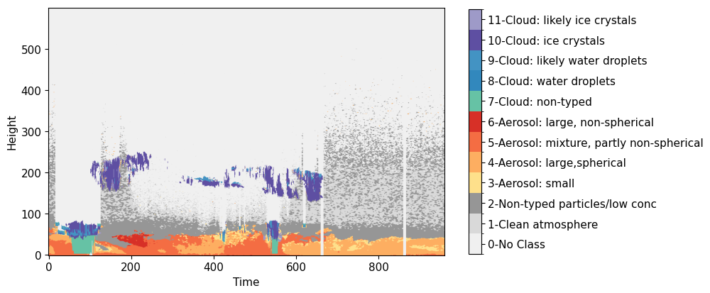
Figure 1 Unified atmospheric target classification mask. A 2D time-height training label for 3 November 2016, created by integrating PollyXT aerosol typing and Cloudnet cloud/precipitation categorization. The vertical axis represents altitude (up to 22.5 km), and the horizontal axis represents 24 h of observations at 90-s resolution. Classes range from clear atmosphere (Class 1) to specific aerosol types (Classes 3–6) and various cloud phases including water droplets and ice crystals (Classes 8–11).

This merging strategy leverages the complementary physical capabilities of both instruments. Cloud radar excels at detecting ice crystals and penetrating dense cloud structures, whereas lidar is highly sensitive to aerosols and optically thin clouds. Consequently, radar classification takes precedence, where applicable, while lidar classification serves as the default in regions without a radar signal. This simple but effective rule preserves the detailed PollyXT aerosol classification, leverages Cloudnet to improve the representation of precipitation and thick clouds, and retains high-altitude ice clouds that are often too weak to exceed the radar's sensitivity threshold. The label classes are numbered as detailed in Table 1, and Fig. 1 shows an example target image that the model aims to learn.

Table 1 Classification Labels.

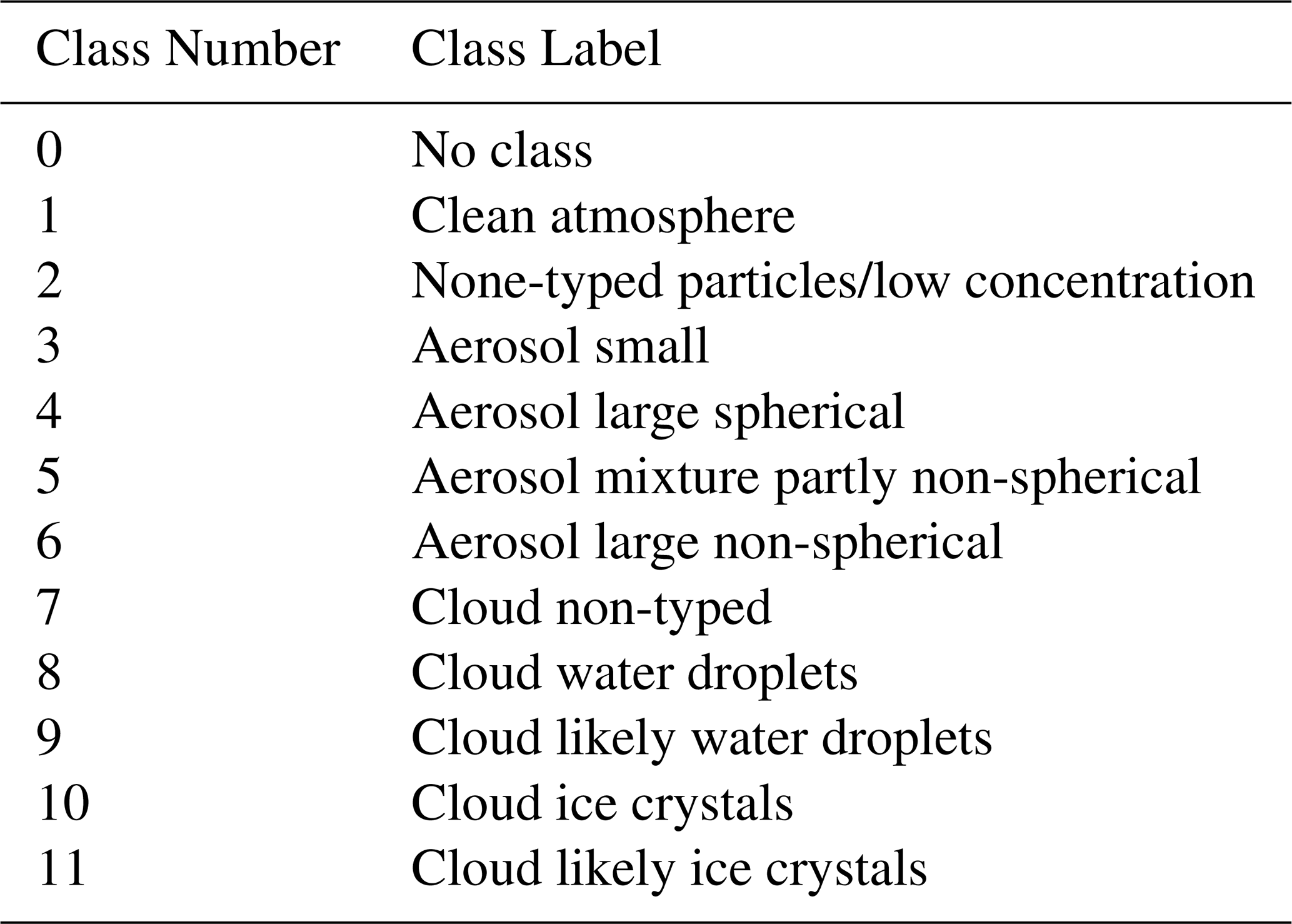
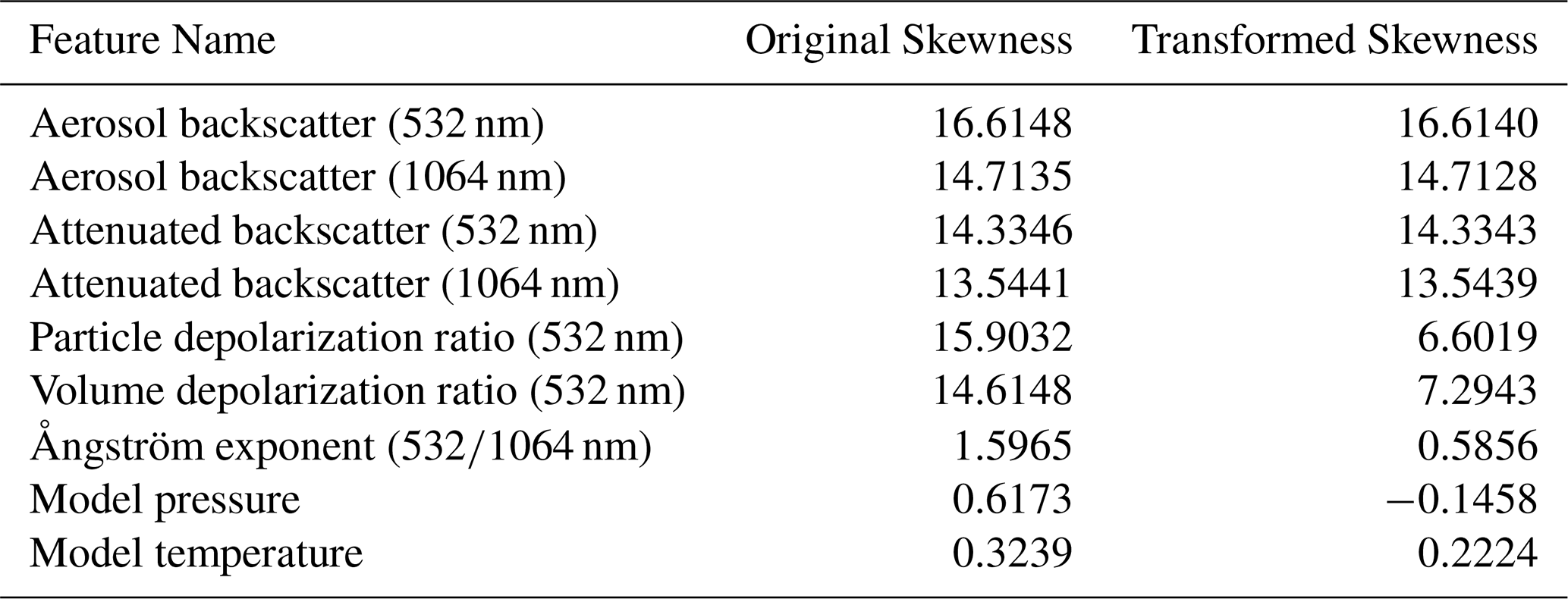
Table 2 Skewness of input features before and after the log (1+x) transformation across the full dataset.

3 Methodology

3.1 Data preprocessing

Prior to ingestion by the U-Net model, the raw lidar data were subjected to a series of preprocessing steps to ensure data quality and suitability for the network architecture. Initially, each input sample was filtered to conform to the expected input dimensions of 600 vertical bins by 960 time steps. Instances containing missing timestamps were identified; since they constituted only 3 % of the entire dataset, these samples were excluded from the training, validation and testing sets. Subsequently, the lidar data were clipped to zero, given that lidar-derived physical quantities such as backscatter and depolarization ratios are inherently non-negative. If negative values exist in lidar data, they typically resulted from instrumental noise or background subtraction procedures, particularly in regions with low signal-to-noise ratios. Next, we addressed NaN entries, which occur in lidar profiles due to factors such as complete signal attenuation in dense clouds, low signal-to-noise ratios in pristine regions, or instrument malfunction. Because neural networks cannot mathematically process NaN values, numerical imputation was a structural necessity. These missing values were replaced using the global average of the respective feature. However, because missing data in lidar often represents a physically meaningful state rather than a mere absence of measurement, it was critical to ensure this gap-filling did not introduce bias. To prevent the model from confusing a physical measurement with an imputed value, we engineered a corresponding binary indicator feature for each input variable. This indicator took a value of 1 if the original data at that specific pixel had been a NaN (and was subsequently imputed), and 0 otherwise. This crucial step provided the model with explicit information about the original data quality at each point, allowing it to reliably learn the distinction between valid signals and physically attenuated regions (Jones, 1996).

To address the highly skewed distributions of lidar signals, which often span several orders of magnitude, a log (1+x) transformation was applied uniformly to the input features. This specific transformation was strictly necessary and chosen over standard logarithmic or square root alternatives. Because the lidar data arrays were clipped to zero to remove instrumental noise, they contain true zero values where log (0) is undefined. The +1 shift safely handles these zero-signal regions without generating artificial missing values, while compressing the dynamic range of high-intensity measurements sufficiently to prevent them from dominating the neural network's loss function. To quantitatively evaluate the effectiveness of this transformation over the full dataset, we calculated the Fisher–Pearson coefficient of skewness (Doane and Seward, 2011), for each feature before and after the transformation:

$${\displaystyle }{\displaystyle }{g}_{\mathrm{1}}={\displaystyle \frac{\frac{\mathrm{1}}{N}{\sum }_{i=\mathrm{1}}^N(x_i-\overline{x}{)}^{\mathrm{3}}}{{\left(\frac{\mathrm{1}}{N}{\sum }_{i=\mathrm{1}}^N(x_i-\overline{x}{)}^{\mathrm{2}}\right)}^{\mathrm{3}/\mathrm{2}}}}$$

where N is the total number of pixels in the dataset, x_i is the individual pixel value, and $\overline{x}$ is the mean of the feature. A skewness value of 0 indicates perfect symmetry. As detailed in Table 2, the raw lidar variables exhibited extreme positive skewness. The transformation successfully reduced this skewness, resulting in more symmetrical, log-normal distributions. Notably, while the transformation heavily compressed the long right tails of certain features (such as the volume depolarization ratio and the backscatter-related Ångström exponent), the backscatter coefficients showed minimal changes in their global skewness metrics. This is an expected mathematical behavior: because backscatter coefficients consist of exceptionally small magnitude values (often on the order of 10⁻⁵), x is close to 0, making $\log (\mathrm{1}+x)\approx x$. Thus, the transformation acts as a safe, near-linear pass-through for these specific channels, preserving their underlying structural variance while stabilizing the broader feature space.

Following the logarithmic transformation, the features were standardized according to:

$${\displaystyle }{z}_i={\displaystyle \frac{x_i-\mathit{\mu }}{\mathit{\sigma }}}$$

where μ and σ were calculated from the log-transformed per-feature training data, and then applied to the validation and test datasets. Standardization transforms the features to have a mean of approximately zero and a standard deviation of approximately one, ensuring that all features contribute more equally to the learning process, preventing domination by features with larger numerical ranges, and promoting faster and more stable training (Ioffe and Szegedy, 2015).

3.2 Learning

The dataset was partitioned into training, validation, and testing subsets in a 70:10:20 ratio, resulting in 284 samples allocated for training, 40 for validation, and 80 for testing. Care was taken to ensure that each subset maintained a similar variance in the distribution of the total distinct number of atmospheric classes present within each sample. For each subset, let I be the set of all samples and c be a specific class. Thus:

$$\begin{array}{ll}{\displaystyle }& {\displaystyle }{I}_c=\mathit{\{}i\in I|\text{ sample }i\text{ contains class }c\mathit{\}}\\ \text{(1)}& {\displaystyle }& {\displaystyle }{\text{Count}}_c=\left|I_c\right|\end{array}$$

We then plot the kernel density estimate (KDE) of each subset and compare the curves to make sure that the distributions behave similarly (Fig. 2). This stratified approach helped ensure that each dataset split was representative of the overall class diversity, preventing potential biases, and ensuring robust model training and evaluation.

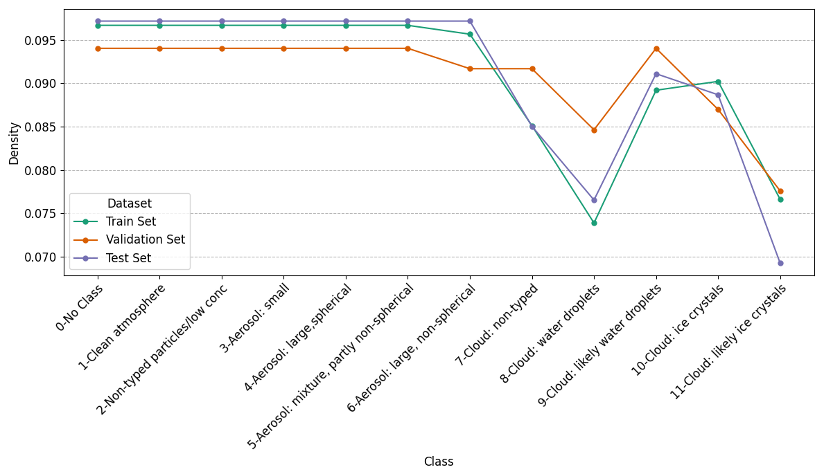
Figure 2 Dataset stratification analysis. Kernel Density Estimate (KDE) plot showing the frequency of the 12 atmospheric classes across the Training (70 %), Validation (10 %), and Test (20 %) subsets. The alignment of the curves ensures that each split is representative of the overall atmospheric diversity, preventing class frequency bias during model evaluation.

A U-Net architecture (Fig. 3) was selected for this task due to its demonstrated success in image segmentation, including applications in earth and atmospheric sciences (Foley et al., 2024) (Rusyn et al., 2019) (Galea et al., 2023) and other applications (Levy-Jurgenson et al., 2020). Its structure is particularly well-suited for tasks requiring both contextual understanding and precise localization. The architecture follows a symmetric encoder-decoder structure with skip connections, tailored to capture both hierarchical features and fine-grained spatial details. The encoder decreases the dimensions of the input and increases the number of feature channels, and the decoder increases the dimensions of the bridge data and decreases the number of feature channels.

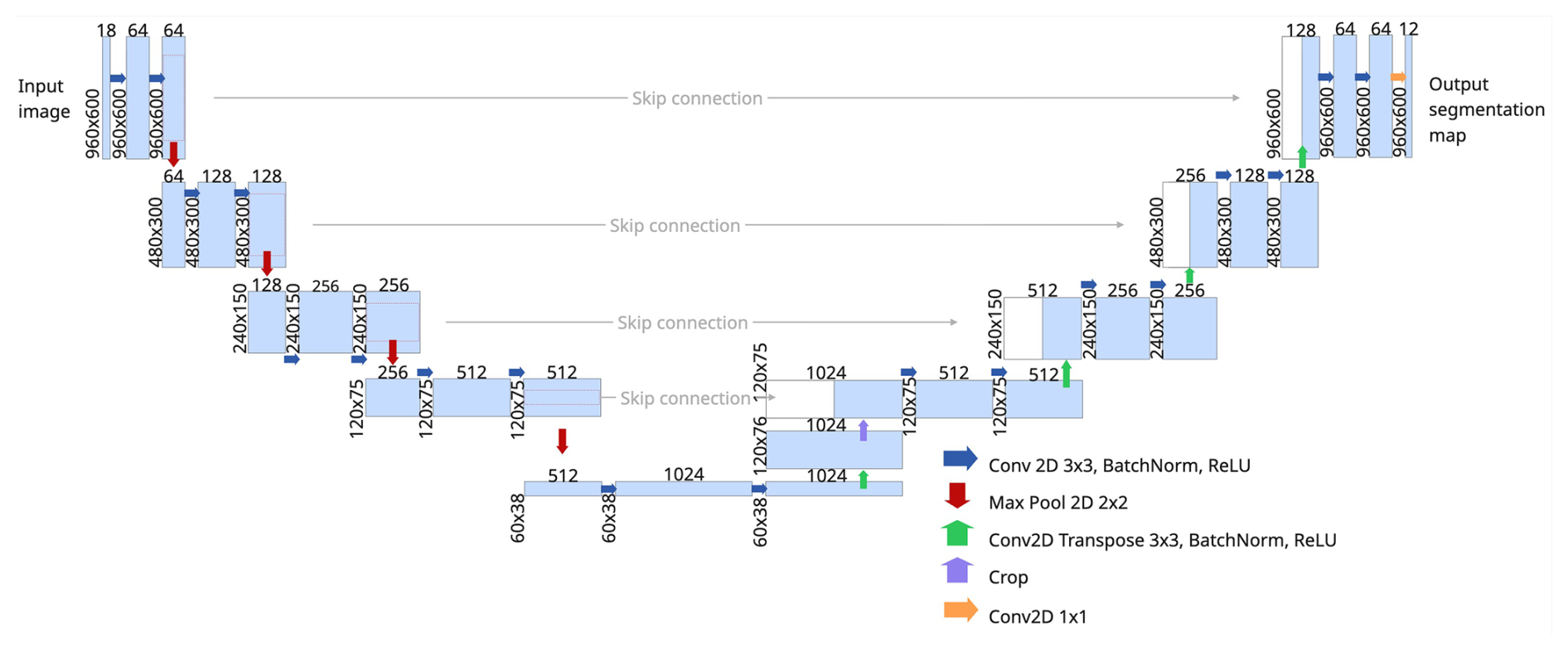
Figure 3 U-Net architecture for pixel-wise atmospheric segmentation. This U-Net-style architecture features an encoder, a bottleneck, and a decoder. The encoder captures context through four downsampling blocks, where each block applies two sequential 3×3 convolution layers (followed by batch normalization and ReLU) with an increasing number of filters (64, 128, 256, 512), a dropout layer with a rate of 0.1, and a final 2×2 max-pooling operation. Feature maps from the encoder are passed to the decoder via skip connections. The central bottleneck layer consists of two 3×3 convolutions with 1024 filters, batch norm, ReLU, and a dropout layer with a rate of 0.2. The decoder path enables exact localization by mirroring the encoder. Each of its four upsampling blocks uses a 2×2 transposed convolution, concatenates its output with the corresponding feature map from the skip connection, and applies two more 3×3 convolutions. The network terminates with a 1×1 convolution and a softmax activation function to generate the final pixel-wise segmentation mask.

To effectively train the U-Net model for our multi-class segmentation task, a composite loss function was employed. This tailored loss function was designed to address two key challenges: achieving accurate segmentation for each individual atmospheric class, many of which are imbalanced, and specifically penalizing confusion between aerosol and clouds. The total loss, L_total, is defined as:

$$\begin{array}{}\text{(2)}& {\displaystyle }{\displaystyle }{L}_{\text{total}}=L_{\text{MWSD}}+\mathit{\lambda }\cdot L_{\text{GC}}\end{array}$$

where L_MWSD is the multiclass weighted squared dice loss, L_GC (described below) is the group confusion loss (Eqs. 3 and 5 respectively). The penalty λ is a penalty factor that balances the contribution of the group confusion term (L_GC – described below). This penalty was a hyperparameter and was optimized based on the best results of the validation set.

Dice coefficient is a common metric for evaluating overlap in segmentation tasks, and its loss variant has proven to be effective, particularly for imbalanced classes (Sudre et al., 2017) (Milletari et al., 2016). To address the inherent imbalance in the frequency of different atmospheric aerosol and cloud types, class weights w_class are introduced (Bressan et al., 2022). These weights were chosen to be inversely proportional to the frequency or volume of each class in the training dataset, thereby giving more importance to underrepresented classes. A multiplicative factor was applied for training stability. A weight of 0 was applied to the first class which is defined as “no-class” (Class 0). This was done to ensure that the model only learns physical features and assigns anything that doesn't fit a physical phenomenon to “no class” (Class 0). The dice coefficient was calculated as follows:

$$\begin{array}{ll}{\displaystyle }& {\displaystyle }{L}_{\text{MWSD}}=\mathrm{1}\\ \text{(3)}& {\displaystyle }& {\displaystyle }-\mathrm{2}\left({\displaystyle \frac{{\sum }_{j=\mathrm{1}}^h{\sum }_{i=\mathrm{1}}^t{y}_t(i,j)\cdot y_p(i,j)\cdot w_c\left(y_t\right(i,j\left)\right)}{{\sum }_{j=\mathrm{1}}^h{\sum }_{i=\mathrm{1}}^t\left(y_t^{\mathrm{2}}\right(i,j)+y_p^{\mathrm{2}}(i,j\left)\right)\cdot w_c\left(y_t\right(i,j\left)\right)}}\right)\text{(4)}& {\displaystyle }& {\displaystyle }{w}_c(i,j)=\mathrm{200}\cdot {\displaystyle \frac{\mathrm{1}}{n_c}}\end{array}$$

where h and t are the height and time indices, y_t are the ground truth labels, y_p are the prediction probabilities, w_c is the scaled inverse frequency of the true training class and n_c is the number of times a specific true class appears in the training dataset. Note that w_c is the weight associated to each class and is a function of y_t.

Although L_MWSD focuses on individual class performance, a critical requirement for this application is to strongly discourage misclassifications between fundamentally different atmospheric categories, specifically between aerosol and clouds. To address this, a group confusion loss term, L_GC is introduced:

$$\begin{array}{}\text{(5)}& {\displaystyle }{\displaystyle }{L}_{\text{GC}}=\sum _{j=\mathrm{1}}^h\sum _{i=\mathrm{1}}^t{y}_{\text{ta}}(i,j)\cdot y_{\text{pc}}(i,j)+y_{\text{tc}}(i,j)\cdot y_{\text{pa}}(i,j)\end{array}$$

where y_ta are the ground truth aerosol labels, y_pc are the predicted cloud probabilities, y_tc are the ground truth cloud labels and y_pa are the predicted aerosol probabilities. The composite loss function (Eq. 5) is designed to guide the U-Net model not only to accurately segment individual aerosol and cloud types (even rare ones, due to weighting in L_MWSD), but also to maintain a clear distinction between the broader aerosol and cloud categories.

The U-Net model was developed and trained using the TensorFlow and Keras libraries. Adam optimization algorithm, with an initial learning rate of $\mathrm{5}\times {\mathrm{10}}^{-\mathrm{3}}$, was employed to minimize the loss function (Eq. 2). To prevent overfitting and reduce unnecessary training time, early stopping was implemented as follows. Validation loss was monitored and training was halted if no improvement was observed for 20 consecutive epochs, starting from epoch 50. The best weights achieved during training (post epoch 50) were restored upon stopping. The learning rate was adaptively adjusted during training. If the validation loss did not improve for 10 epochs, the learning rate was reduced by a factor of 0.2, down to a minimum learning rate of $\mathrm{5}\times {\mathrm{10}}^{-\mathrm{7}}$. This allows for finer adjustments as the model approaches convergence. Training was implemented using Tensorflow on Google Cloud Vertex AI, Colab Enterprise notebook, using NVIDIA TESLA A100x4 GPUs.

4 Results and discussion

In this section, we present the quantitative and qualitative evaluation of the trained U-Net model. We first assess its overall classification accuracy and class-specific performance across the test dataset, followed by detailed case studies demonstrating its behavior under complex atmospheric conditions.

Model training stopped after 167 steps due to the early stopping mechanism, where epoch 148 was chosen as the best epoch with a training loss value of 0.1198 and a validation loss value of 0.1288. Jaccard index at the chosen epoch was 0.9009 for the training set and 0.5955 for the validation set, and cloud-aerosol confusion loss was 0.0023. Both loss values and Jaccard indices for the training and validation sets plateaued at around step 120, where the most significant learning was done between steps 0 and 60. Results henceforth will be discussed solely regarding the test dataset, which comprises 80 samples that the model has not seen. The model's performance was quantitatively assessed using metrics such as precision, recall, and F1-score for each atmospheric class:

$$\begin{array}{ll}\text{(6)}& {\displaystyle }& {\displaystyle }P\left(i\right)={\displaystyle \frac{\text{TP}\left(i\right)}{\text{TP}\left(i\right)+\text{FP}\left(i\right)}}\text{(7)}& {\displaystyle }& {\displaystyle }R\left(i\right)={\displaystyle \frac{\text{TP}\left(i\right)}{\text{TP}\left(i\right)+\text{FN}\left(i\right)}}{\displaystyle }& {\displaystyle }\text{F1}\left(i\right)=\mathrm{2}\cdot {\displaystyle \frac{P\left(i\right)\cdot R\left(i\right)}{P\left(i\right)+R\left(i\right)}}\\ \text{(8)}& {\displaystyle }& {\displaystyle }={\displaystyle \frac{\text{TP}\left(i\right)}{\text{TP}\left(i\right)+\frac{\mathrm{1}}{\mathrm{2}}\left(\text{FP}\right(i)+\text{FN}(i\left)\right)}}\end{array}$$

where TP, FP, and FN are the true positive, false positive and false negative results, and where i represents the class. To determine the overall performance of the model, the macro-averaged F1-scores, weighted macro-averaged F1-scores, and micro F1-scores were calculated:

$$\begin{array}{ll}{\displaystyle }& {\displaystyle }{\text{F1}}_{\text{macro}}={\displaystyle \frac{{\sum }_{i=\mathrm{1}}^{\mathrm{12}}\text{F1}\left(i\right)}{\mathrm{12}}},\\ {\displaystyle }& {\displaystyle }{P}_{\text{macro}}={\displaystyle \frac{{\sum }_{i=\mathrm{1}}^{\mathrm{12}}P\left(i\right)}{\mathrm{12}}},\\ \text{(9)}& {\displaystyle }& {\displaystyle }{R}_{\text{macro}}={\displaystyle \frac{{\sum }_{i=\mathrm{1}}^{\mathrm{12}}R\left(i\right)}{\mathrm{12}}},{\displaystyle }& {\displaystyle }{\text{F1}}_{\text{weighted}}=\sum _{i=\mathrm{1}}^{\mathrm{12}}{w}_i\text{F1}\left(i\right),\\ {\displaystyle }& {\displaystyle }{P}_{\text{weighted}}=\sum _{i=\mathrm{1}}^{\mathrm{12}}{w}_{i}P\left(i\right),\\ \text{(10)}& {\displaystyle }& {\displaystyle }{R}_{\text{weighted}}=\sum _{i=\mathrm{1}}^{\mathrm{12}}{w}_{i}R\left(i\right),{\displaystyle }& {\displaystyle }{\text{F1}}_{\text{micro}}=\\ {\displaystyle }& {\displaystyle \frac{{\sum }_{i=\mathrm{1}}^{\mathrm{12}}\text{TP}\left(i\right)}{{\sum }_{i=\mathrm{1}}^{\mathrm{12}}\text{TP}\left(i\right)+\frac{\mathrm{1}}{\mathrm{2}}\left({\sum }_{i=\mathrm{1}}^{\mathrm{12}}\text{FP}\right(i)+{\sum }_{i=\mathrm{1}}^{\mathrm{12}}\text{FN}(i\left)\right)}}\\ {\displaystyle }& {\displaystyle }{P}_{\text{micro}}={\displaystyle \frac{{\sum }_{i=\mathrm{1}}^{\mathrm{12}}\text{TP}\left(i\right)}{{\sum }_{i=\mathrm{1}}^{\mathrm{12}}\text{TP}\left(i\right)+{\sum }_{i=\mathrm{1}}^{\mathrm{12}}\text{FP}\left(i\right)}}\\ \text{(11)}& {\displaystyle }& {\displaystyle }{R}_{\text{micro}}={\displaystyle \frac{{\sum }_{i=\mathrm{1}}^{\mathrm{12}}\text{TP}\left(i\right)}{{\sum }_{i=\mathrm{1}}^{\mathrm{12}}\text{TP}\left(i\right)+{\sum }_{i=\mathrm{1}}^{\mathrm{12}}\text{FN}\left(i\right)}}\end{array}$$

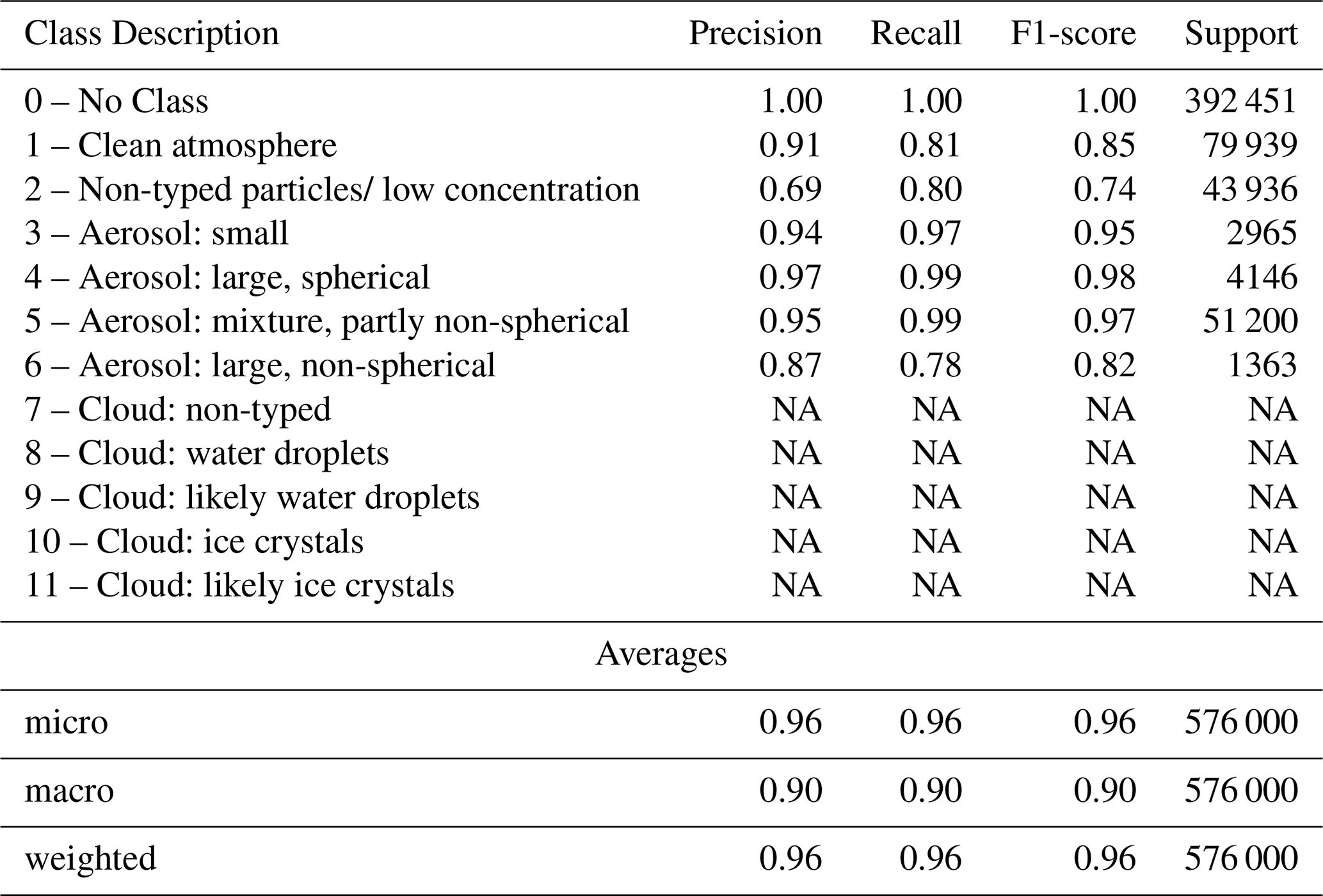
where i runs on all classes, and w_i is the fraction of that class within the entire test dataset, and TP, FP, FN are the sum of the true positive, false positive and false negative results. The evaluation is based on the test dataset, which comprises 46 080 000 individual pixel classifications in all test samples, and is detailed in Table 3.

Table 3 Classification Performance Metrics.

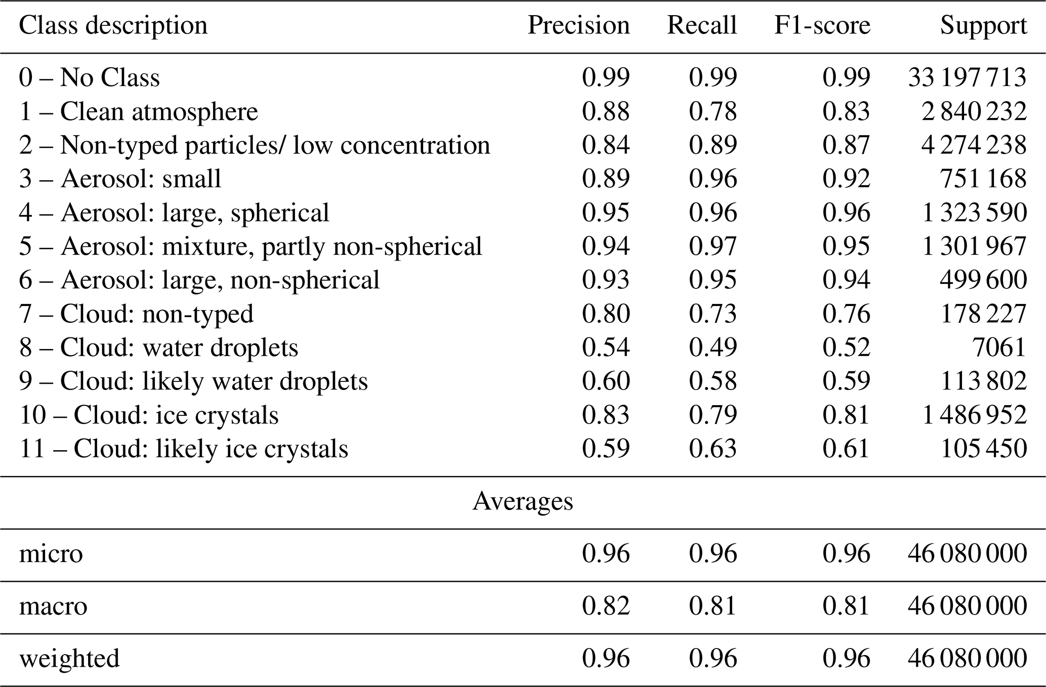
Support = number of pixels pertaining to the corresponding truth class.

4.1 Analysis of Model Performance

The model achieved consistent performance across classes, with a micro-average (Eq. 11) as well as weighted averages (Eq. 10) for accuracy, precision, recall, and F1-score of 0.96. These results indicate that, when class imbalances are taken into account, the classification is reliable and unbiased toward specific categories. However, the macro average (Eq. 9), which calculates the metric independently for each class and then averages them assuming equal weights, shows more moderate results: a precision of 0.82, recall of 0.81, and an F1-score of 0.81. The difference between the weighted and macro averages points to class imbalance, where the model performs well on the aerosol classes which are more common, but struggles more with cloud classes which are more rare.

The confusion matrix (Fig. 4) provides a granular view of the model's classification accuracy and error patterns. The diagonal elements represent the percentage of correctly classified pixels (recall) for each class. Key aerosol types are classified with high recall rates: “Aerosol: small” (96 % recall), “Aerosol: large, spherical” (96 % recall), “Aerosol: mixture, partly non-spherical” (97 % recall), and “Aerosol: large, non-spherical” (95 % recall). This indicates that the model successfully learned to distinguish the nuanced lidar signatures corresponding to different aerosol properties, like size and shape. There is some minor confusion between aerosol types, such as 1 % of “Aerosol: large, spherical” being misclassified as “Non-typed particles,” and 2.9 % of “Aerosol: large, non-spherical” being misclassified as “Aerosol: mixture.” This is expected, as atmospheric aerosol populations are often complex mixtures rather than discrete types.

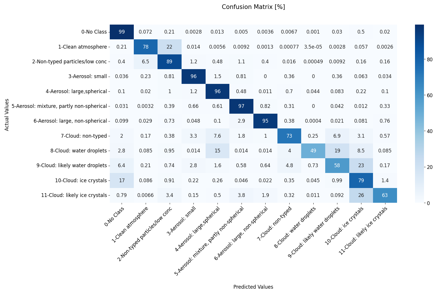
Figure 4 Comprehensive model performance matrix. Normalized confusion matrix for the test dataset. Diagonal elements represent the recall for each class, showing high accuracy for aerosol types (89 %–95 %). The matrix highlights physically plausible confusion between liquid cloud categories (Classes 8 and 9) and the model's high precision in identifying the “No Class” background.

The classification of cloud types reveals a more complex challenge. While the model correctly identifies “Cloud: ice crystals” (Class 10) in 79 % of cases, its performance on liquid water clouds is notably lower. Only 49 % of “Cloud: water droplets” (Class 8) are correctly identified, and 58 % of “Cloud: likely water droplets” (Class 9) are correctly identified. An important observation is the confusion between similar and physically adjacent classes. For “Cloud: water droplets” (Class 8), while the recall is low (49 %), a significant portion of the misclassifications go to neighboring liquid cloud classes: 19 % are mislabeled as “Cloud: likely water droplets” (Class 9) and 4 % as “Cloud: non-typed” (Class 7). Similarly, for “Cloud: likely ice crystals” (Class 11), the main source of error is misclassification as “Cloud: ice crystals” (26 %). This pattern of confusion is physically plausible. Distinguishing between definite and “likely” water droplets, or between droplets and small ice crystals near the freezing level, can be ambiguous even for synergistic algorithms, let alone for a model relying only on lidar.

“No Class” (class 0) is identified with 99 % F1-score, which is very high given that the model was trained with a corresponding weight of 0 in the loss function. This is due to the fact that the U-Net's final layer is a convolution layer with 12 classes and a softmax activation function. The softmax function forces the model to output a probability distribution across all 12 classes for every pixel, and these probabilities must sum to 1. Thus, even if class 0 has zero weight in the loss, the model must still assign some probability to the channel corresponding to class 0 for every pixel. As the model improves in identifying and segmenting classes 1–11, it learns the features and contexts associated with them. For pixels that do not exhibit strong features of any of classes 1–11, the probabilities assigned by the softmax to these classes will naturally be low. Thus, the “leftover” probability mass is often assigned to the remaining classes, which in this case includes class 0. If class 0 is a general “background” or “none of the above specific particle types,” this can lead to it being correctly predicted for those pixels. In addition, class 0 is much more prevalent than other classes (Table 3).

To further investigate the model's capabilities and limitations, Jaccard index was calculated for each height index across the test dataset, excluding the dominant “No Class” category (Eq. 12):

$$\begin{array}{}\text{(12)}& {\displaystyle }{\displaystyle }J={\displaystyle \frac{\text{TP}}{\text{TP}+\text{FP}+\text{FN}}}\end{array}$$

Figure 5 shows the resulting relationship between classification performance and altitude. The general trend aligns with the physical expectations of lidar performance: the highest Jaccard values (0.4–0.6) are concentrated in the lowest height indices (approximately 0–100). Performance gradually degrades through indices 100–300 and becomes poorest at high altitudes (indices >300), where Jaccard values drop below 0.2. This vertical decline in performance is primarily attributable to the smaller number of classes present at higher altitudes (portrayed by the darker colors). Given that the model trained on fewer examples at higher altitudes, we would expect to see lower accuracy at those heights. Furthermore, the decline in performance may also be caused by the degradation of the lidar's signal-to-noise ratio with increasing altitude and the significant signal attenuation caused by intervening clouds and dense aerosol layers. An interesting and seemingly counterintuitive trend is observed in the lowest part of the atmosphere (height indices 0–50). Within this range, where the pixel count is highest (indicated by the lighter color of the points), the mean Jaccard value shows a slight decrease with decreasing height. This is contrary to the assumption that performance should be uniformly best where the lidar signal is strongest and where there are more examples to train on.

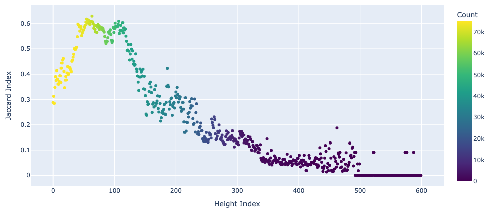
Figure 5 Vertical profiles of classification reliability. The Jaccard Index (Intersection over Union) plotted as a function of height index, with points colored by the total pixel count (Support) at that altitude. Peak performance occurs in the free troposphere (indices 0–100), with degradation at higher altitudes caused by reduced signal-to-noise ratios and signal attenuation from intervening cloud layers.

4.2 Case studies to test model performance

To provide a qualitative assessment of the performance of the model, and to better understand its behavior under specific atmospheric conditions, we analyze a series of case studies from the test set. Each case compares the ground truth classification with the model's prediction and examines a corresponding confusion heatmap to identify specific areas and types of misclassification. The results of the case studies are summarized in Table 4.

Table 4 F1-scores for Single Image Case Studies (1–3).

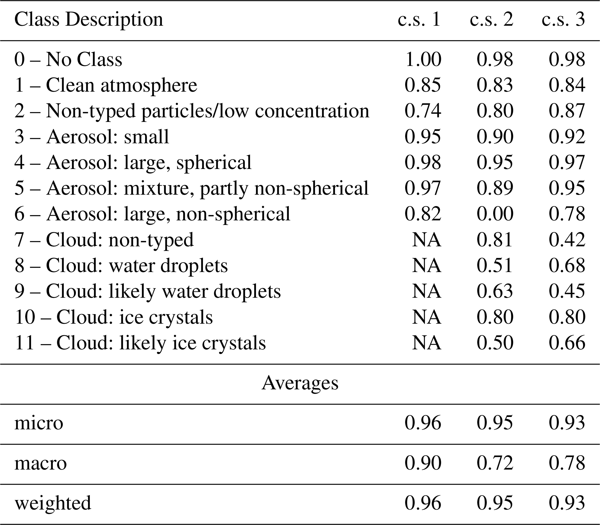
NA: not available.

4.2.1 Case 1: Cloud-free multiple layering conditions

The first case study (7 December 2016) examines a complex, cloud-free scene with several distinct aerosol layers (Fig. 6). This scenario serves as a validation of the model's ability to classify aerosols. Given that the target classification is done using only lidar data, we expect the model to perform well. The model successfully captures the vertical extent, boundaries, and temporal evolution of the different aerosol layers. The “Aerosol: mixture, partly non-spherical” (Class 5) layer is accurately reproduced by the model in both its location and classification. “Large, non-spherical” class is also correctly identified in the time steps between 200–450 and 800–960. Furthermore, the model also correctly identifies the overlying layer of “non-typed particles/low concentration” (Class 2) and the “clean atmosphere” (Class 1) above it. The per-image classification report confirms this strong performance with a weighted F1-score of 0.96. The most prevalent class, “Aerosol: mixture, partly non-spherical,” achieves an F1-score of 0.97. Other aerosol classes also show high F1-scores, such as “Aerosol: large, spherical” (0.98) and “Aerosol: small” (0.95).

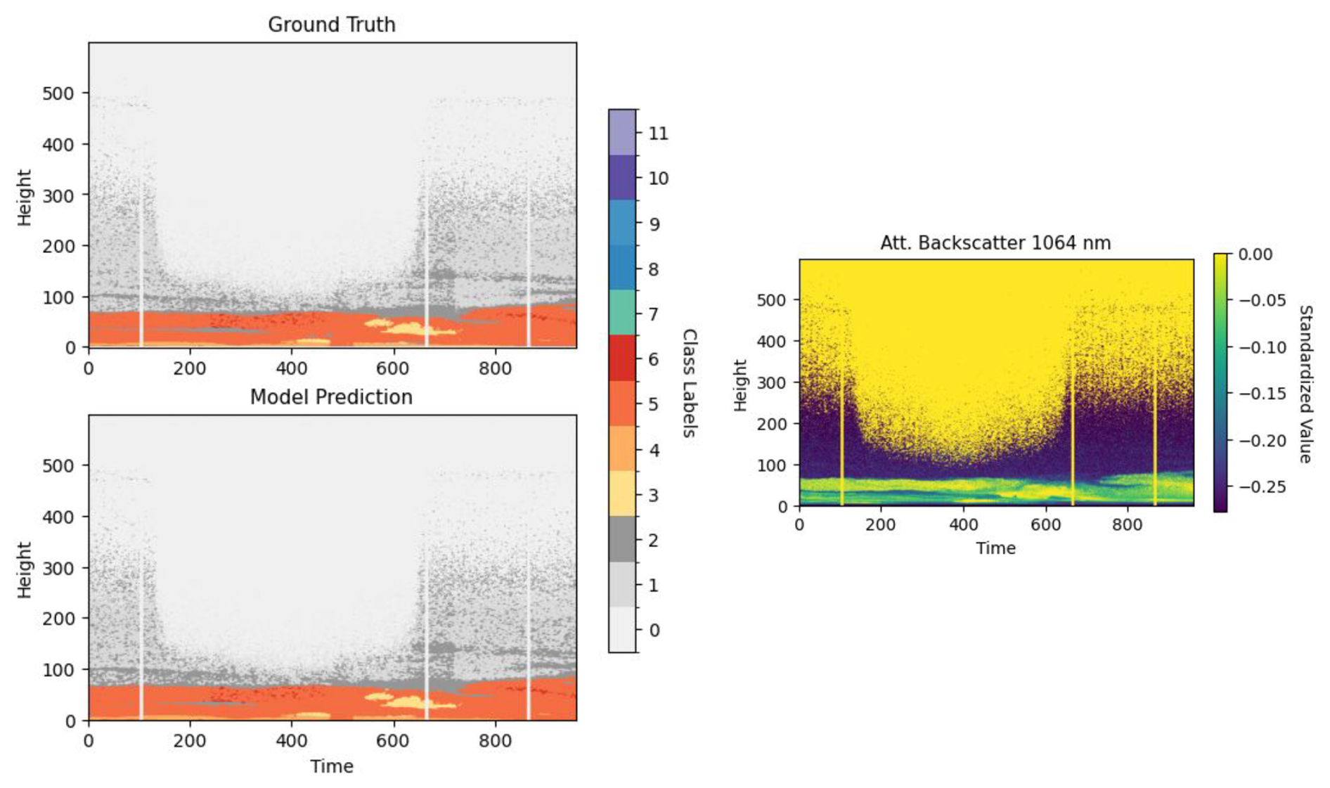
Figure 6 Case study 1: cloud free, distinct aerosol layers qualitative comparison. Side-by-side comparison showing the ground truth labels and the U-Net model's predictions (left) alongside the corresponding attenuated backscatter (right) for 10 September 2017.

The confusion matrix (Fig. A4) shows only minor, physically reasonable errors, such as overlap between “Clean atmosphere” and “Non-typed particles” and some confusion of “Aerosol: small” with “Aerosol: mixture.” Notably, the group confusion heatmap (Fig. A1) indicates no aerosol–cloud misclassifications in this case. These results indicate that the composite loss function improved discrimination, with the group confusion term reducing aerosol–cloud ambiguity and enabling clear separation between the two categories in this case. Furthermore, The generalized confusion heatmap (Fig. A1) shows only minor ambiguity, mainly between closely related aerosol types (e.g. Class 5 within Class 4). This case study illustrates the model's ability to resolve aerosol subtypes in cloud-free conditions.

4.2.2 Case 2: Aerosol-cloud interaction study

The second case study investigates the interaction between a near-surface aerosol layer and an overlying liquid cloud (13 November 2016). This case directly tests the model's ability to delineate the boundary between aerosol and cloud and to correctly classify both in close proximity. As in the previous case, the model's prediction shows a very good structural agreement with the ground truth (Fig. 7). It accurately identifies the general location and extent of the low-level aerosol layer (primarily “Aerosol: large, spherical”) and the cloud system above it (a mix of “likely water droplets” and “ice crystals”). The temporal evolution of both features is also well replicated.

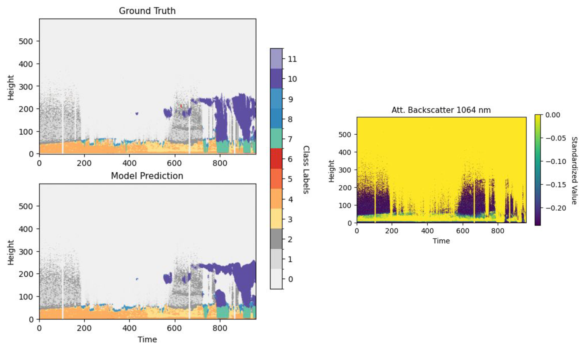
Figure 7 Case study 2: low level liquid cloud and aerosol layers qualitative comparison. Side-by-side comparison showing the ground truth labels and U-Net model's predictions (left) alongside the attenuated backscatter (right) for 13 November 2016.

The Confusion Heatmap highlights that the most significant misclassifications are concentrated precisely at this boundary. This indicates that while the model can identify the core of the aerosol and cloud layers, it struggles to precisely delineate the transition zone between them. The Aerosol-Cloud Group Confusion Density Heatmap (Fig. A2) reveals distinct, though localized, instances of confusion between aerosol and cloud groups. These areas are co-located with the aerosol-cloud interface shown in the main plots. This indicates that the majority of the model's errors in this scene are aerosol-cloud misclassifications. The confusion matrix (Fig. A5) quantifies this: for example, 7.5 % of “Cloud: non-typed” (Class 7) is misclassified as “Aerosol: large, spherical” (Class 4). Most notably, the entire class of “Aerosol: large non-spherical” (Class 6) was misclassified and was primarily confused with Class 10 and Class 11 (a mix of “likely water droplets” and “ice crystals”). However, due to it's temporal-spacial singularity, where it only appears in one timestamp and at a specific height index, and due to its small support of only 54 pixels (Table A2), it is safe to disregard these results as anomalous.

4.2.3 Case 3: Mid–High Clouds and Low-Level Dust Event

The last case study explores a complex multilayered cloud system that stretches from mid to high altitudes, with an air quality event (dust storm) at low altitudes, which took place on the date 15 January 2017. This case was chosen to test whether the model can predict clouds correctly at high altitudes at the very limit of lidar attenuation. The ground truth plot (Fig. 8) shows a mid-level “Cloud: likely water droplets” (Class 9) layer at height index 200, where directly below and above it are classes 10 and 11 (ice clouds). The model's prediction correctly identifies the low-level aerosol and liquid cloud layers with good structural accuracy. Most importantly, it successfully infers the presence of the upper-level ice cloud in a position and with a structure that closely matches the ground truth. It is important to note that classifications assigned above the altitude of complete lidar signal attenuation do not represent direct observations, but probabilistic inferences based on the vertical structure below the cloud top and thermodynamic constraints learned from the training dataset. The per-image classification report shows a strong F1-score of 0.80 for “ice crystals” (Class 10), which make up the bulk of the upper cloud. This quantitatively confirms the model's successful inference. However, the confusion heatmap (Fig. A3) reveals errors concentrated at the top and bottom boundaries of the inferred ice cloud. The per-image confusion matrix (Fig. A6) shows that 23 % of “likely ice crystals” are misclassified as “ice crystals,” a plausible and minor error. Critically, the “Aerosol/Cloud Group Confusion Density Heatmap” remains predominantly dark, indicating that even in this complex multi-layer, multi-phase scene, the model rarely confuses the fundamental aerosol and cloud categories.

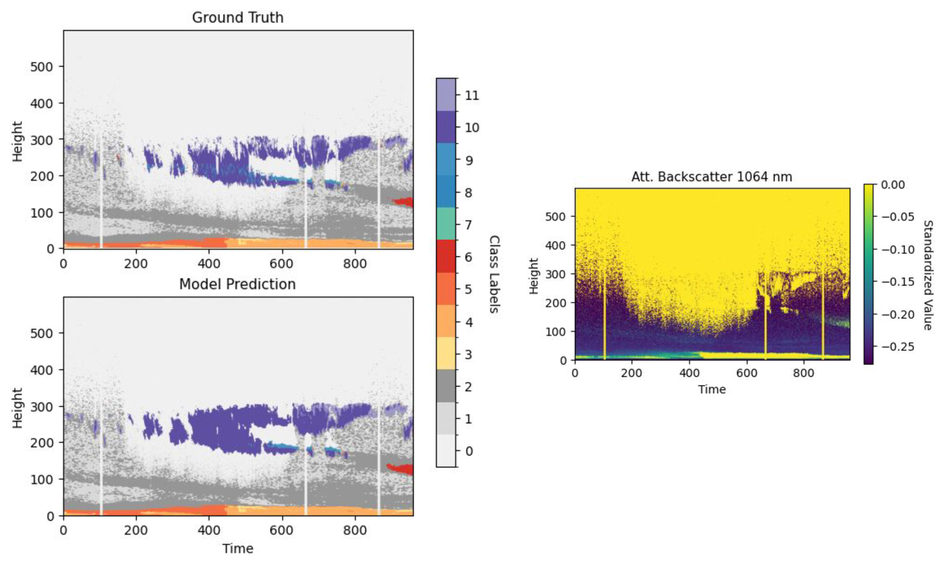
Figure 8 Case study 3: mid–high clouds and low-Level dust event qualitative comparison. Side-by-side comparison showing the ground truth labels and the U-Net model's predictions (left) alongside the corresponding attenuated backscatter (right) for 15 January 2017.

5 Concluding Remarks

This study investigated a novel deep learning approach for unified aerosol and cloud classification using only ground-based lidar data. The approach is motivated by the need for comprehensive atmospheric composition profiling and the inherent limitations of lidar-only retrievals (primarily signal attenuation in clouds). The high-quality datasets generated by Cloudnet are indispensable and serve as the robust ground truth required to train our supervised machine learning framework. Our objective was not to replace Cloudnet's multi-instrument infrastructure, but to use it to infer the presence of convective clouds, which facilitates cloud screening and establishing basic cloud occurrence statistics. This approach bridges the gap between the critical need for vertical cloud maps and the sparse global availability of full Cloudnet stations, allowing sites equipped only with standard lidars to benefit from approximated Cloudnet-like classifications. A U-Net architecture was developed and trained, where the model takes standard lidar measurements (attenuated backscatter, depolarization ratio) as input and aims to predict a detailed vertical classification encompassing both aerosol types (PollyXT outputs) and cloud/precipitation categories (Cloudnet outputs).

The deep learning model developed in this study demonstrated significant capability in classifying atmospheric constituents from lidar data alone. The model achieves excellent overall performance (weighted F1-score of 0.96) and is particularly adept at classifying diverse aerosol types. In cloud-free conditions, it successfully distinguishes between different aerosol categories with high recall rates, validating its ability to learn the subtle signatures associated with particle size and shape based on the input lidar features. Crucially, this approach positions our contribution distinctly within the current state of the art. Recent advancements, such as the multitask machine learning framework of Fuller et al. (2025), have demonstrated the efficacy of deep learning for cloud-aerosol typing using space-based lidar. However, because those models train on datasets derived solely from lidar measurements, they remain physically constrained by lidar signal attenuation and cannot classify features where the signal is extinguished. Our model overcomes this limitation by utilizing ground truth aligned with Cloudnet and PollyXT standards, which incorporate cloud radar data. Since radar penetrates thick optical layers, our training data set includes atmospheric information invisible to lidar. This allows the model to learn contextual correlations and approximate a lidar-radar synergy from a single lidar input, inferring properties above the attenuation limit, which is an operational advancement beyond purely lidar-trained architectures.

The model exhibits strong predictive capabilities in identifying ice clouds (F1-score of 0.81) but struggles more with classifying specific liquid cloud categories, particularly the rare “water droplets” class. The observed confusion between similar classes (e.g. “water droplets” and “likely water droplets”) is physically reasonable and highlights the inherent ambiguity in defining discrete boundaries for continuous atmospheric processes. The use of a composite loss function, which features a group confusion penalty, proved effective in minimizing the most critical classification errors. Across all case studies, including complex multi-layer and multi-phase scenes, the model consistently and reliably discriminated between the broader categories of aerosol and clouds, with confusion being rare and localized to the most ambiguous interface regions. Model performance varies predictably with altitude, achieving optimal results in the free troposphere, where signals are strong and targets are well-defined. Performance degrades at high altitudes due to decreasing signal-to-noise ratio and at very low altitudes in part due to instrumental effects and the high complexity of the planetary boundary layer.

Despite the potential, several limitations and challenges must be acknowledged. The performance of the deep learning model is fundamentally dependent on the quality, accuracy, and representativeness of the complex training dataset. Any biases or errors inherent in the reference PollyXT and Cloudnet algorithms used to generate the target variable will likely be learned and propagated by the U-Net model. Further more, a model trained on data from one specific site or lidar instrument, as is the case in this study, may not perform equally well and may not generalize in different atmospheric regimes or with data from different lidar systems without either retraining or the application of domain adaptation techniques.

The findings of our study have important implications for atmospheric remote sensing, suggesting that ground-based observational systems could be simplified. By applying advanced algorithms to relatively simple and cost-effective lidar data, it may be possible to reduce the reliance on co-located, complex, and expensive instruments such as cloud radars and microwave radiometers, thereby facilitating the establishment of denser observational networks (Illingworth et al., 2007). Such networks could provide valuable data streams for improving weather forecasts, evaluating climate models (particularly concerning cloud feedback and ACI), and supporting air quality and environment monitoring as well as aviation safety.

We are planning future work to focus on further exploring different deep learning architectures, including variants of the U-Net or transformer-based models. Exploring physics-informed neural networks, which incorporate physical constraints into the learning process, might also improve the physical consistency of the predictions. Validation efforts using independent datasets could further build confidence and establish generalization capabilities. This includes data from different geographical locations, seasons, and lidar instruments. Comparison with data from field campaigns involving airborne in-situ measurements or overpasses of satellites with cloud-penetrating capabilities would provide valuable independent validation as well. Although our model successfully infers structures beyond the attenuation limit, quantifying the exact signal threshold required for valid reconstruction remains an important open question for future studies. Additionally, conducting a comprehensive quantitative ablation study to measure the precise performance impact of removing individual input variables could help decrease the complexity of the model to allow faster inference and model training times.

Appendix A: Case Studies

Table A1 Classification Performance Metrics for case study 1 – Complex Multi-Layer Aerosol.

NA: not available.

Table A2 Classification Performance Metrics for case study 2 – Low Level Liquid Cloud and Aerosol.

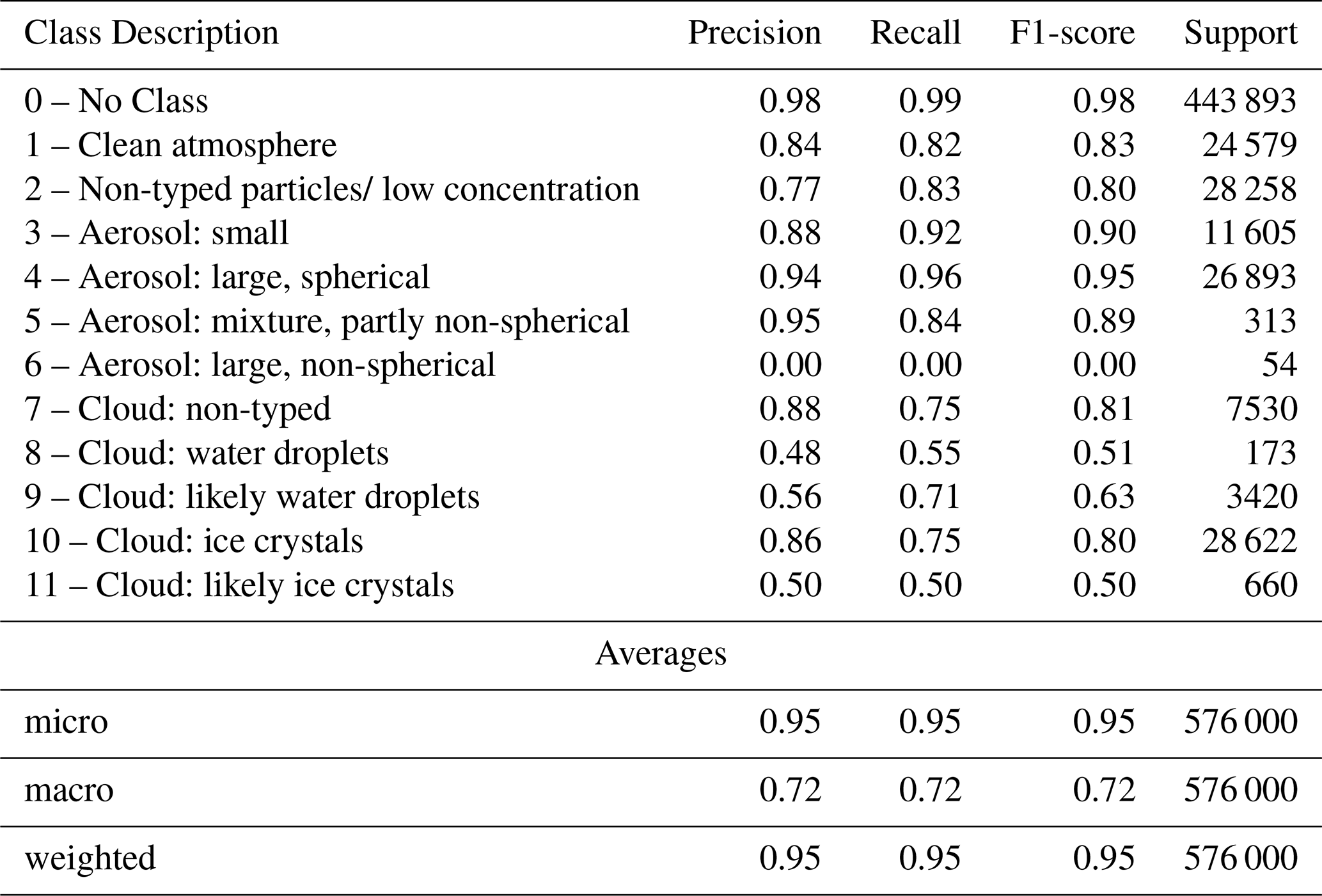
Table A3 Classification Performance Metrics for case study 3 – Lidar Signal Attenuation.

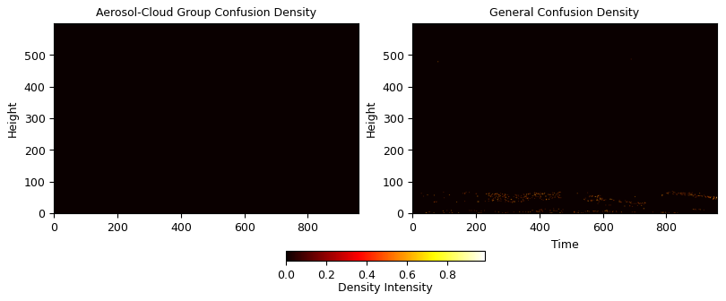
Figure A1 Case study 1 – spatial distribution of classification errors. (Left) Group confusion density heatmap highlighting specific regions where the model confuses the broad categories of aerosols and clouds. (Right) Generalized confusion heatmap excluding background and clean atmosphere classes (0–2) to visualize the nuances of subtype misclassification.

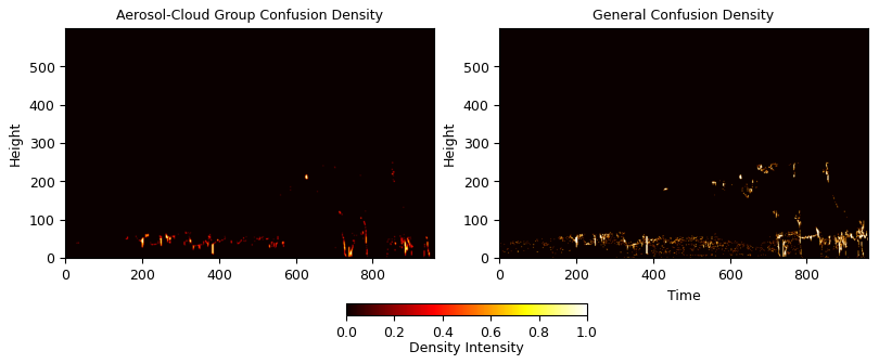
Figure A2 Case study 2 – spatial distribution of classification errors. (Left) Group confusion density heatmap highlighting specific regions where the model confuses the broad categories of aerosols and clouds. (Right) Generalized confusion heatmap excluding background and clean atmosphere classes (0–2) to visualize the nuances of subtype misclassification.

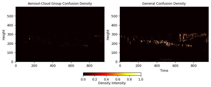
Figure A3 Case study 3 – spatial distribution of classification errors. (Left) Group confusion density heatmap highlighting specific regions where the model confuses the broad categories of aerosols and clouds. (Right) Generalized confusion heatmap excluding background and clean atmosphere classes (0–2) to visualize the nuances of subtype misclassification.

Figure A4 Confusion matrix for case study 1 – Complex Multi-Layer Aerosol.

Figure A5 Confusion matrix for case study 2 – Low Level Liquid Cloud and Aerosol.

Figure A6 Confusion matrix for case study 3 – Lidar Signal Attenuation.

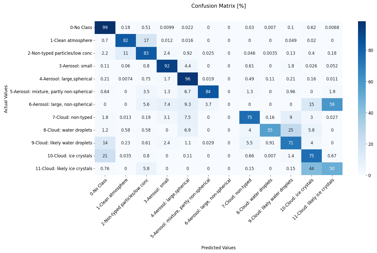
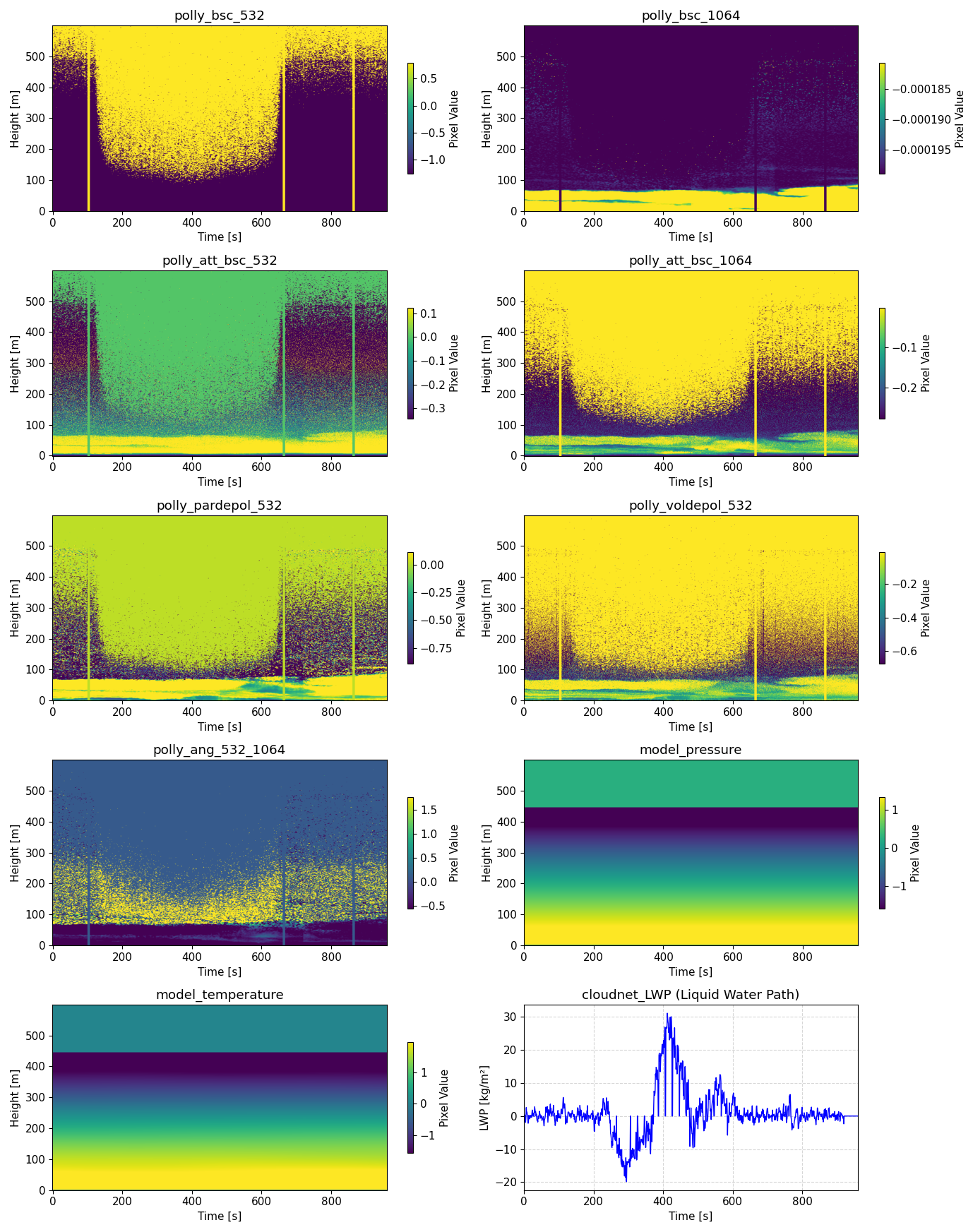
Figure A7 Raw signals case study 1 – Input lidar and meteorological feature suite. Visualization of the multi-channel input data used by the U-Net, including attenuated and aerosol backscatter ($\mathrm{532}/\mathrm{1064}$ nm), depolarization ratios, the backscatter-related Ångström exponent, NWP-derived pressure/temperature profiles and liquid water path. These raw signals (excluding LWP) provide the hierarchical features necessary for the model to infer atmospheric state even in signal-attenuated regions.

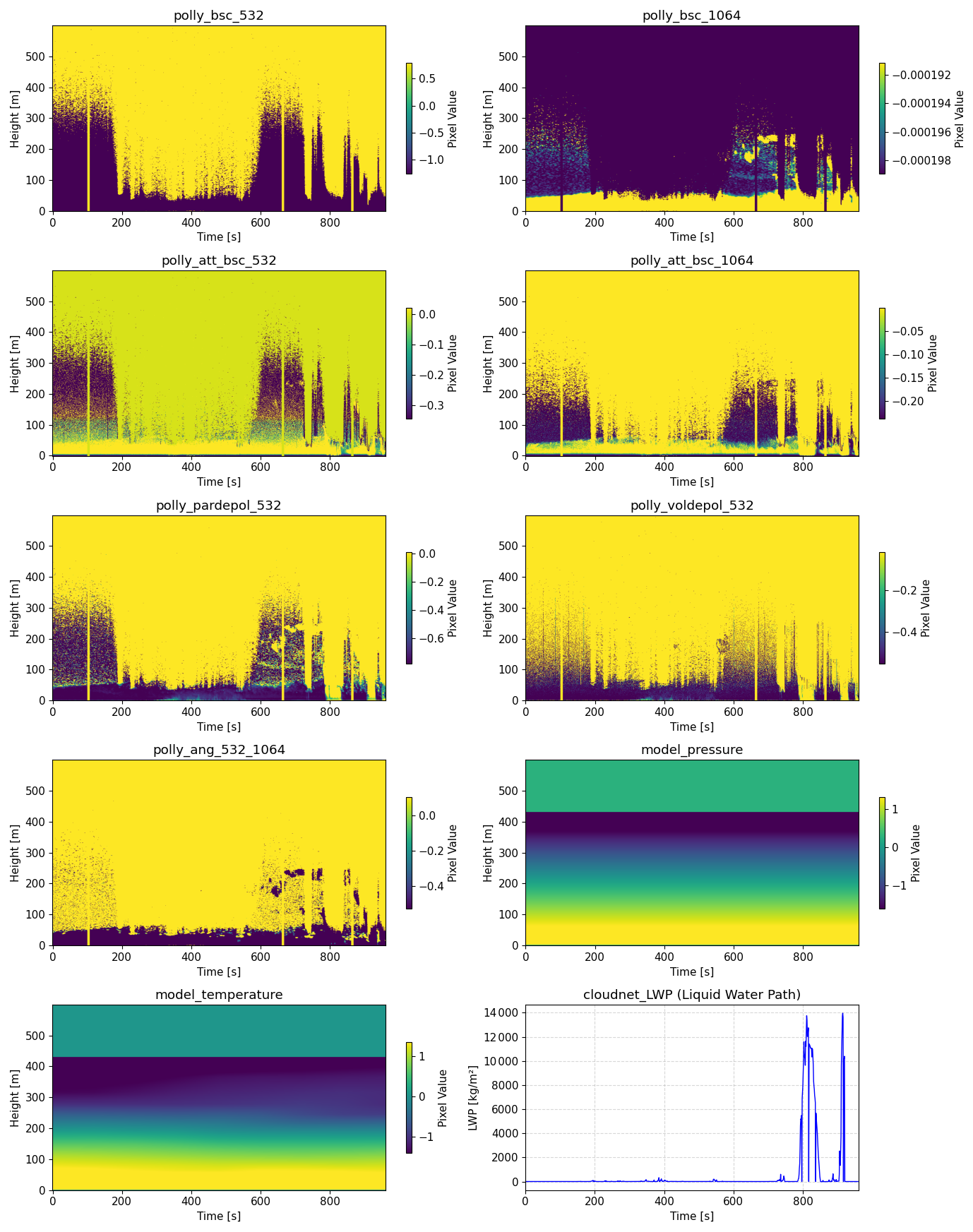
Figure A8 Raw signals case study 2 – Input lidar and meteorological feature suite. Visualization of the multi-channel input data used by the U-Net, including attenuated and aerosol backscatter ($\mathrm{532}/\mathrm{1064}$ nm), depolarization ratios, the backscatter-related Ångström exponent, NWP-derived pressure/temperature profiles and liquid water path. These raw signals (excluding LWP) provide the hierarchical features necessary for the model to infer atmospheric state even in signal-attenuated regions.

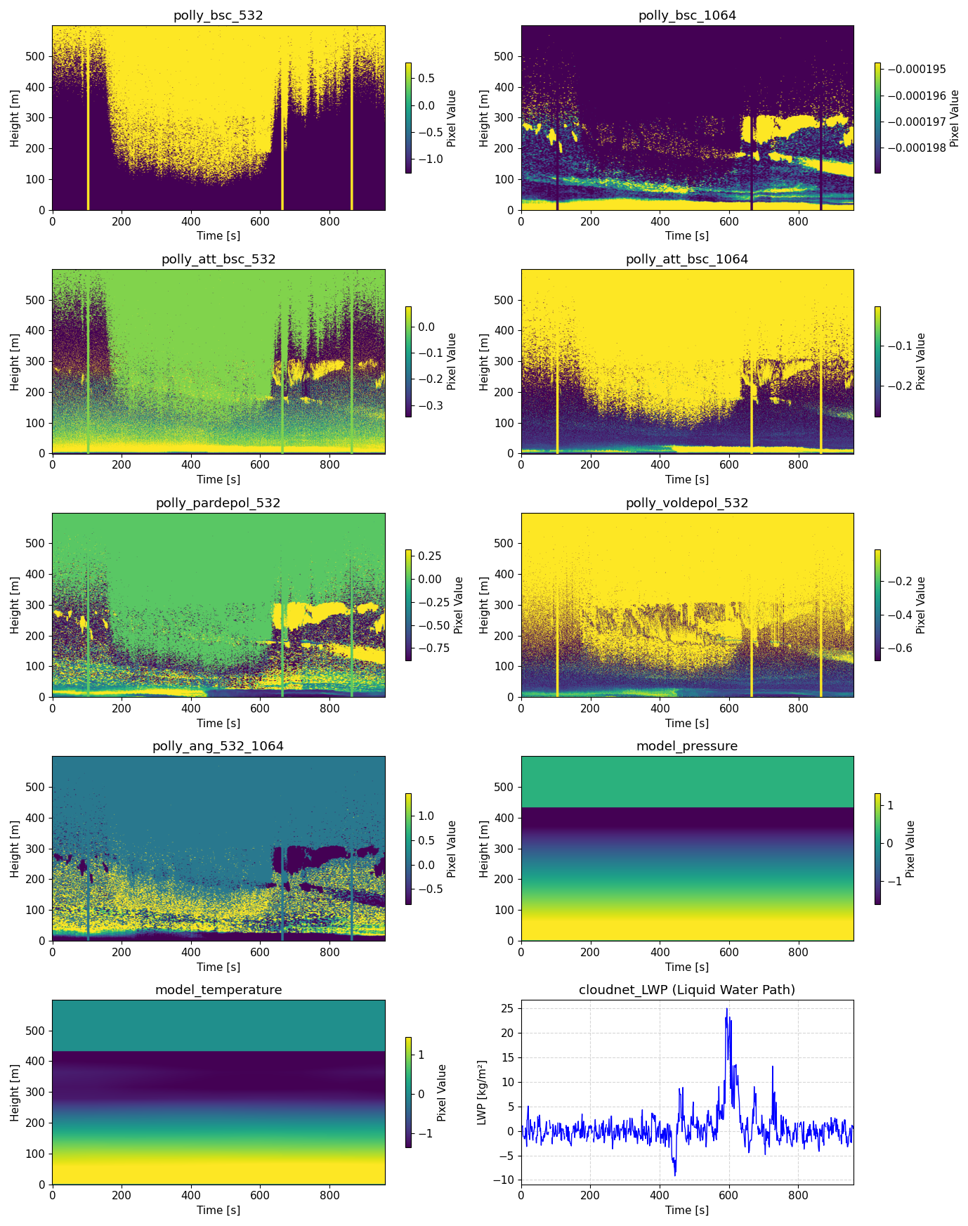
Figure A9 Raw signals case study 3 – Input lidar and meteorological feature suite. Visualization of the multi-channel input data used by the U-Net, including attenuated and aerosol backscatter ($\mathrm{532}/\mathrm{1064}$ nm), depolarization ratios, the backscatter-related Ångström exponent, NWP-derived pressure/temperature profiles and liquid water path. These raw signals (excluding LWP) provide the hierarchical features necessary for the model to infer atmospheric state even in signal-attenuated regions.