Fugitive natural gas emissions in York, United Kingdom: updating the parameters of existing algorithms to be based on instrumental limitations

Reducing methane (CH₄) emissions has become increasingly important in recent years due to its importance for radiative forcing. Fugitive emissions of CH₄ from natural gas distribution infrastructure are of particular interest as a mitigation target within the oil and gas sector. Previous studies have shown the ability to detect these emissions by use of mobile surveys measuring CH₄, with some studies using ratios to secondary co-emitted compounds as a means of predicting the source of emission. This study aims to adapt existing algorithm parameters by investigating the limitations of equipment within the platform used for mobile surveys. These changes suggest that previous methods may underpredict the number of Leak Indications (LIs) by 53.5 % with 27 LIs detected with the old methodology compared to 58 LIs detected with the new methodology. The majority of these LIs were found to be emitting in a leak rate category of 0–2 L min⁻¹. Source determination was included as a core step within the algorithm, which was shown to reduce the misassignment of LIs, suggesting when not using this step, emissions from pyrogenics and biogenics are included within LI assignments.

1 Introduction

Following COP26 and the Global Methane Pledge (European Commission and United States of America, 2021), CH₄ and its emissions have received increased attention. The pledge states that the signatories will attempt to reduce their CH₄ emissions by 30 % of their 2020 levels by 2030. This was brought about due to increasing concern over the potency of CH₄ as a greenhouse gas, with its warming potential 28 times greater than CO₂ over a 100 year timescale and 84 times greater over a 20 year timescale (IPCC, 2021). Anthropogenic sources are estimated to contribute to 65 % of all CH₄ emissions, with atmospheric CH₄ seeing a consistent growth rate of >5 ppb yr⁻¹ since 2007, with 2021 and 2022 seeing growth rates of 17.8 and 14 ppb yr⁻¹ respectively (Saunois et al., 2025). Therefore, understanding and mitigating anthropogenic CH₄ is a key step in complying with the Global Methane Pledge.

Of anthropogenic emissions, the agricultural sector has the largest contribution towards atmospheric emissions (Saunois et al., 2025). Although there are means of reducing these emissions, such as changes to cattle, crop and land management as well as changing the feedstock of the cattle, from grass silage to maize silage (Bačėninaitė et al., 2022; Nisbet et al., 2025). These changes may still require time to implement, so this sector cannot be the sole focus in order to reach the 2030 deadline.

After agriculture, the largest contributor to anthropogenic emissions is the energy sector, with oil, natural gas and coal having relatively similar contributions to CH₄ emissions. Natural gas is of particular importance to the United Kingdom (UK), which is the 19th largest country emitter of CH₄ from the natural gas network (Scarpelli et al., 2022).

One of the major sources of CH₄ emissions from the natural gas network is fugitive emissions. A fugitive emission is an unexpected or unwanted emission of gas from a pressurised network that is not detected by standard means (Sotoodeh, 2021). Within the natural gas network, fugitive emissions are commonly referred to as “gas leaks”. However, the stigma surrounding this term, both from industrial operators and the public, means the term fugitive emission is preferable to be used where possible.

In the UK in 2023, 63.5×10⁹ m³ of natural gas was consumed (Energy Institute, 2024). This is used in a range of applications, including industrial use, electricity generation and domestic use. Of the UK's natural gas consumption, 33.8 % is from the domestic sector (DESNZ, 2024), with 73.8 % of households in England and Wales using mains gas for either heating or cooking purposes (Stewart and Bolton, 2024). In 2022, it was estimated that 117 kT of CH₄ was emitted as a result of fugitive emissions related to natural gas distribution (NAEI, 2025).

Within the UK, after natural gas is either produced or imported, it is first transported through National Gas' National Transmission System (NTS), a network of over 8000 km of high-pressure steel pipes and more than 500 above ground installations. Natural gas is then transported by one of the UK's Gas Distribution Networks (GDNs), a GDN first reduces the pressure from the NTS then oversees the pipework for pre-meter distribution of natural gas to homes and businesses. The GDN responsible for York covers 2.7 million homes and businesses across the northeast of England and northern Cumbria, resulting in tens of thousands of kilometres of pipework and therefore large uncertainties in the locations of fugitive emissions. To combat this, previous studies have implemented mobile measurement approaches centred around the detection of areas with elevated CH₄.

1.1 Previous Mobile Measurement Methodology

Multiple previous studies have attempted to design algorithms to detect fugitive emissions of natural gas, all of which focus on locating enhancements in CH₄, the major component of natural gas. These algorithms define an enhancement based on whether CH₄ mixing ratios are higher than a certain value (Phillips et al., 2013), above a certain percentile in measured readings (Hopkins et al., 2016, Chamberlain et al., 2016) or by using an outlier detection model (Keyes et al., 2020).

The paper upon which our methodology is based (von Fischer et al. 2017), defines Observed Peaks (OPs) as CH₄ enhancements >110 % of a 2.5 min rolling background of the mean CH₄ concentrations two minutes before and after each measured point. Additionally, OPs must not cover a distance greater than 160 m. Enhancements occurring within 5 s of each other are grouped together. Mobile surveys are repeated multiple times and Leak Indications (LIs) are determined by grouping OPs that occur within 20 m of one another and determining which of these grouped clusters contain OPs from more than one mobile survey. The LIs are then quantified into emission rates in L min⁻¹, using an equation derived from the results of a controlled release experiment, shown in Eq. (1).

$$\begin{array}{}\text{(1)}& \begin{array}{rl}(\text{release rate}& /\mathrm{L}{\min }^{-\mathrm{1}})=\mathrm{0.1178}+\mathrm{0.08267}\times M\\ & -\mathrm{0.005175}\times A+\mathrm{0.08626}\times K\end{array}\end{array}$$

where:

• M is the maximum CH₄ reading

• A is the peak area in ppm m

• K is the ratio of ppm m to maximum CH₄

This methodology was further developed in Weller et al. (2019), where the baseline became the median CH₄ value over 2.5 min, the spatial grouping of OPs to LIs changed from 20–30 m and the quantification equation changed to Eq. (2).

$$\begin{array}{}\text{(2)}& \begin{array}{rl}\ln (\text{excess}& {\mathrm{CH}}_{\mathrm{4}}/\mathrm{ppm})=-\mathrm{0.988}\\ & +\mathrm{0.817}\times \ln (\text{emission rate}/\mathrm{L}{\min }^{-\mathrm{1}})\end{array}\end{array}$$

Where the excess CH₄ term is the mean of all CH₄ enhancements associated with the resulting LI.

In Maazallahi et al. (2020), it was proposed that the existing methodology categorised certain burning emissions as fugitive emissions. To counter this, an additional stage using CO₂ ratios with CH₄ was introduced to filter out burning emissions.

Source attribution was also used in Fernandez et al. (2022), using isotopic measurements of CH₄ in addition to ethane : methane (C₂:C₁) ratios.

Most recently in Tettenborn et al. (2025), the approach was changed further, adapting the quantification equation to be based on peak area as opposed to peak height, resulting in the quantification equation shown in Eq. (3),

$$\begin{array}{}\text{(3)}& \begin{array}{rl}(\text{release rate}& /\mathrm{L}{\min }^{-\mathrm{1}})=\\ & \exp (\mathrm{1.292}\times \ln (\text{peak area})-\mathrm{2.377})\end{array}\end{array}$$

where ln (peak area) is the mean ln(peak area) of all OPs within the LI cluster.

Variations of this algorithm have been used in many major cities across the USA and Canada (Ars et al., 2020; Weller et al., 2022), Europe (Defratyka et al., 2021; Fernandez et al., 2022; Wietzel and Schmidt, 2023; Vogel et al., 2024) and Asia (Joo et al., 2024, Ueyama et al., 2025, Umezawa et al., 2025). This paper attempts to detect smaller enhancements of methane by adapting detection and clustering parameters to be specific to the limitations of the instrumentation used. The paper also explores the effect of introducing a source attribution filter at the OP stage of the algorithm and how this affects the number and the magnitude of LIs.

2 Methodology

2.1 Instrumentation

The Wolfson Atmospheric Chemistry Laboratories (WACL) Air Sampling Platform (WASP) detailed in Wagner et al. (2021) is the base for these measurements. The sampling inlet for the WASP is located at the front of the van on the driver's side, meaning that the vehicle will sample the centre of the road regardless of direction of travel. Since publication of Wagner et al. (2021), the WASP has been updated to include a Quark-Elec QK-AS07-0183 for GPS readings. For the measurements surrounding natural gas, the WASP was equipped with a Los Gatos Microportable Greenhouse Gas Analyser (MGGA) for measurements of CH₄ and CO₂, Iterative CAvity enhanced Differential optical absorption spectrometer (ICAD) for measurements of NO_x (NO₂+NO), and an Aerodyne Tuneable Infrared Laser Direct Absorption Spectrometer (TILDAS) laser trace gas analyser for measurements of ethane (C₂H₆) (Yacovitch et al., 2014). Measurements of C₂H₆ were calibrated using a three point calibration of a high standard (17.5 ppb), medium (2.5 ppb) and a zero, where calibration standard concentrations were confirmed via GC-MS. For each mobile survey a calibration was performed before and after the mobile survey itself, a linear regression was performed to find the slope and intercept of the calibration concentrations versus measured concentrations. The average of the two calibrations was taken to account for instrument drift during the mobile survey and the resulting equation, Eq. (4), was used to apply a correction to C₂H₆ concentrations,

$$\begin{array}{}\text{(4)}& {\mathrm{C}}_{\mathrm{2}}{\mathrm{H}}_{\mathrm{6}\mathrm{corrected}}={\mathrm{C}}_{\mathrm{2}}{\mathrm{H}}_{\mathrm{6}\mathrm{uncorrected}}\cdot m+c\end{array}$$

Where:

• m = Gradient of calibration concentration vs. mean response averaged over the two calibrations

• c = Intercept of calibration concentration vs. mean response averaged over the two calibrations

2.1.1 Instrument Response Time

Response time of the MGGA is reported as <0.5 s from the manufacturer's specification. The response rate of the TILDAS however was unknown. The TILDAS is capable of recording measurements at a rate of 10 Hz, however, the flow rate through the instrument needed to be altered to make these measurements true to the 10 Hz values. Originally, the inlet to the TILDAS had two valves in series, a stainless steel integral bonnet needle valve, 0.37 Cv, 1/4 in. #SS-1RS4 and an electronic upstream flow control valve, 10 000 sccm, 0.25 in. tube, viton seal #0248A-10000SV which allows small changes to maintain the internal pressure at 70 Torr. With the two valves in series, the instrument was unable to achieve a high enough flow rate for true 10 Hz measurements. Moving the valves to be parallel, the instrument was able to achieve a flow rate close to 5 Hz, which indicated that the pump was the limiting factor for the flow rate of the instrument.

These changes to increase the flow rate of the instrument were made to allow for a response time as close to that of the MGGA as possible. To find the accurate response time of the TILDAS, an experiment was devised whereby a high concentration of C₂H₆ (17.630±0.715 ppb, measured via GC-MS) was flowed through the TILDAS and switched to ambient air 10 times, on 2 separate valve setups, for a total of 20 repeats of low-high-low transitions in the concentration of C₂H₆. The transition times were located by eye and then the transition time to go from 90 % of the maximum value to 10 % of the maximum value was calculated (Symonds, 2017). An example of the high to low transition with the 90 % and 10 % limits is shown in Fig. 1. The transition time on the first valve ranged from 0.7–1.1 s with a mean value of 0.9 s, the second valve had responses ranging from 0.7–1.4 s, also with a mean response of 0.9 s, giving confidence in a sub 1 s response rate from the TILDAS and therefore showing the capability of a sub 1 s response in both instruments. The data however was still averaged to 1 s with a 1 s clustering time due to the data being limited by the data acquisition rate of the WASP's GPS.

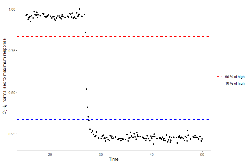
Figure 1 Example response transition of TILDAS high concentration to low concentration, normalised to maximum recorded response.

2.1.2 Variation in methane measurements

Previous algorithms define an enhancement as being higher than 1.1 times a 2.5 min rolling median background. This work however seeks to understand if this parameter holds true for the specific instrumentation used in the mobile surveys. To understand what this parameter may be, a variance experiment was undertaken. The standard deviation of CH₄ measurements over a 2 h period was calculated to understand the minimum detectable enhancement for the CH₄ detection algorithm.

For 2 h compressed air flowed through the Los Gatos MGGA, with an observed median measured value of 7.2 ppm and a standard deviation of 0.006 ppm. An enhancement criteria was proposed as 5 times this standard deviation divided by the median baseline, resulting in an enhancement criteria of 1.005 times the baseline. However, this assumes a stable baseline that is replicated in the field. In reality, when applying this enhancement criteria, it led to the detection of enhancements that were too small to be reliably quantified. Instead, the CH₄ mixing ratios measured during each mobile survey were collated and the standard deviation was calculated for each mobile survey. Enhancement criteria was calculated as anything larger than 5 times the standard deviation divided by the median CH₄ mixing ratios. This was repeated for each mobile survey and resulted in a median enhancement criteria of 1.01 times the baseline. However, as this could result in detection of very small, diffuse, or non-natural gas emission enhancements, a larger enhancement criteria of 1.05 times the background was selected. This ensured there was still a large difference from the original methodologies criteria, while still remaining within the known variation of the instrumentation.

2.2 Driving Route

York is a city in the north-east of England with a population over 200 000. A driving campaign took place over two separate weeks in May and June 2024 resulting in 18 mobile surveys of a “flower petal” route, shown in Fig. 2, staying within the outer ring roads of the A64 and A1237 and focused primarily on sampling residential areas of the city. The majority of the roads sampled on the route were only driven in one direction, but due to the position of the sampling inlet this allowed the middle of the road to be sampled regardless of the direction of travel. The route was driven 18 times as, in order to capture >90 % of emissions, a route should be driven at least 5–8 times over separate days (Luetschwager et al., 2021). The route was chosen as it covers multiple different neighbourhoods within York, but was not intended to be used to compare measurements to the cities emissions inventory as it only covers a small fraction of the total miles of road within the York urban area, 27 mi of a total 507 administered by the local authority (Department for Transport, 2025).

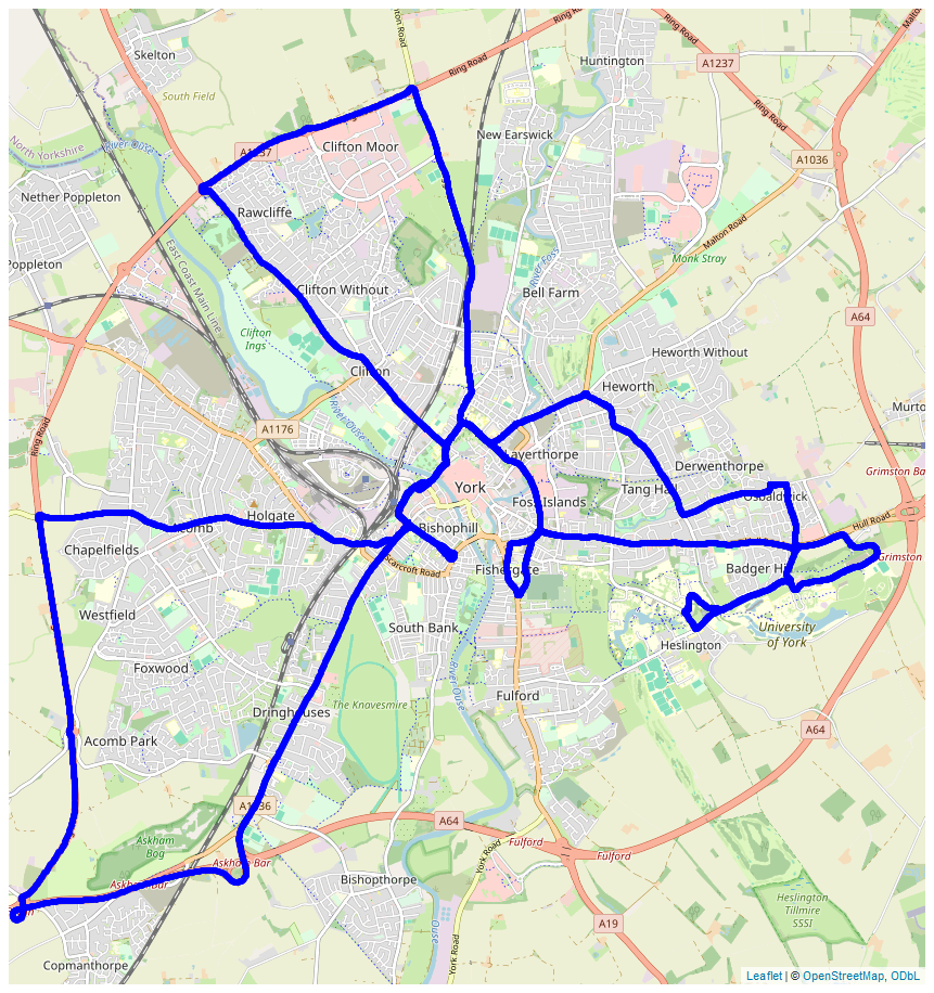
Figure 2 Map of the route taken in WASP surveys. Produced using leaflet (Cheng et al., 2025) with tiles taken from OpenStreetMap (© OpenStreetMap contributors https://www.openstreetmap.org/copyright, last access: June 2026).

2.3 Enhancement Detection Algorithm

The original algorithm, used in Weller et al. (2019), was adapted following the findings in Sects. 2.1.1 and 2.1.2. OPs were clustered within 1 s as opposed to 5 s. With a faster instrument response, it was expected that the measurements would more readily distinguish between two separate enhancements that occurred spatially close to one another. By clustering over a time of 5 s, assuming an average speed of 20 mi h⁻¹ (8.9 m s⁻¹), this would mean the potential to cluster together enhancements 44.5 m apart, whereas a cluster time of 1 s would at most be clustering enhancements 8.9 m apart, the reason for this change was discussed in Sect. 2.1.1. Enhancement criteria was also changed, instead of an enhancement needing to be more than 110 % of the baseline, it must be 105 % of the baseline. This allows detection of smaller enhancements, this change was discussed in Sect. 2.1.2. LI determination occurred after identifying the source type of each OP, ensuring LI analysis occurred only on OPs of the thermogenic source type, to further reduce the chance of comparing long standing thermogenic fugitive emissions with possible nearby single occurrence pyrogenic or biogenic emissions.

2.4 Controlled Release Experiment

To obtain a quantification equation specific to the equipment used in York, a controlled release experiment was conducted at the Bedford Aerodrome over 5 d in May 2024. A MiniCRF was deployed to manage releases of CH₄ and ammonia (NH₃), while a MidiCRF was deployed for releases of C₂H₆. In total, there were 41 releases lasting an average of 30 min each. Releases consisted of varying amounts of CH₄ (0.2–70.48 L min⁻¹), C₂H₆ (0–7.01 L min⁻¹) and NH₃ (0–7.87 L min⁻¹) to reflect a range of CH₄ emission sources, including natural gas and farm emissions. Releases were from a mixture of linear vertical releases, a multi emission point ring, multi point source emissions and single point releases, occurring at heights ranging from ground level to 3 m elevation. Over the course of the experiment wind speeds were measured using four Gill Met Pak Pro instruments deployed at 3, 6, 9 and 12 m elevation, winds were recorded as 1 min vector averages. Average wind speed over the 5 d was 3.87 m s⁻¹ with wind speeds ranging from 0–9.75 m s⁻¹. During each release, an initial period was spent locating the plume before sampling the plume at set distances for 10 repeats, the platform then moved further away in distance for another set of 10 repeats. This continued until the plume was either lost, or a lack of driveable ground was left available. It was noted that larger releases were detectable further away, however, as the data from the controlled release was intended to be used in quantifying under-road and near-road fugitive emissions of natural gas, a maximum distance of 30 m from the point of release was applied for data analysis to reflect the maximum road widths typically found within a city like York (Essex Planning Officers Association, 2018).

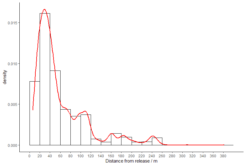
Figure 3 Density plot of number of detected enhancements during the controlled release campaign against distance from release point.

Of the 41 releases conducted in the controlled release, only 26 releases were able to be used for data analysis due to several reasons, including that some releases did not have detectable enhancements. Within these 26 releases, 3525 CH₄ enhancements were detected over distances between 5.8 and 382.1 m from the release point; the majority of releases detected further away from the release point were from higher emission rate releases. When enhancements were filtered to a maximum distance of 30 m from the release point, this resulted in 1226 enhancements from 23 releases. Density plots of the number of detected enhancements against distance from source are shown in Fig. 3 for all detected enhancements and Fig. 4 for enhancements detected within 30 m from the source.

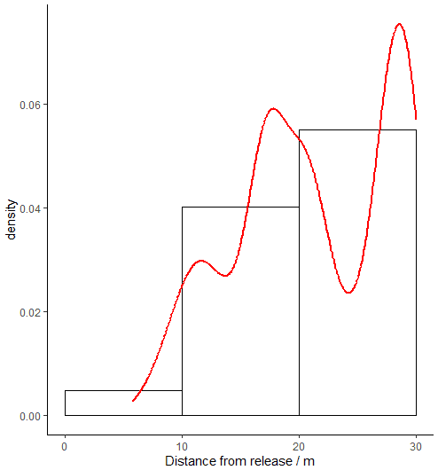
Figure 4 Density plot of number of detected enhancements during the controlled release campaign against distance from release point (Limited to 0–30 m).

2.4.1 Quantification equation

There has been much development and advancement in the last few years on the use and application of “advanced mobile leak detection” systems for natural gas emissions detection and reporting. The original methodologies, where algorithms were developed to convert peak height maxima of measured methane plumes to estimated emission rates (Weller et al., 2019) have been superseded with plume area algorithms (Tettenborn et al., 2025) which are instrument and vehicle speed agnostic. However, this is still not a precise conversion and can only be treated as a generalised guide to emissions estimation due to external factors such as wind, instrument inlet location and local variability due to buildings and unknown source locations.

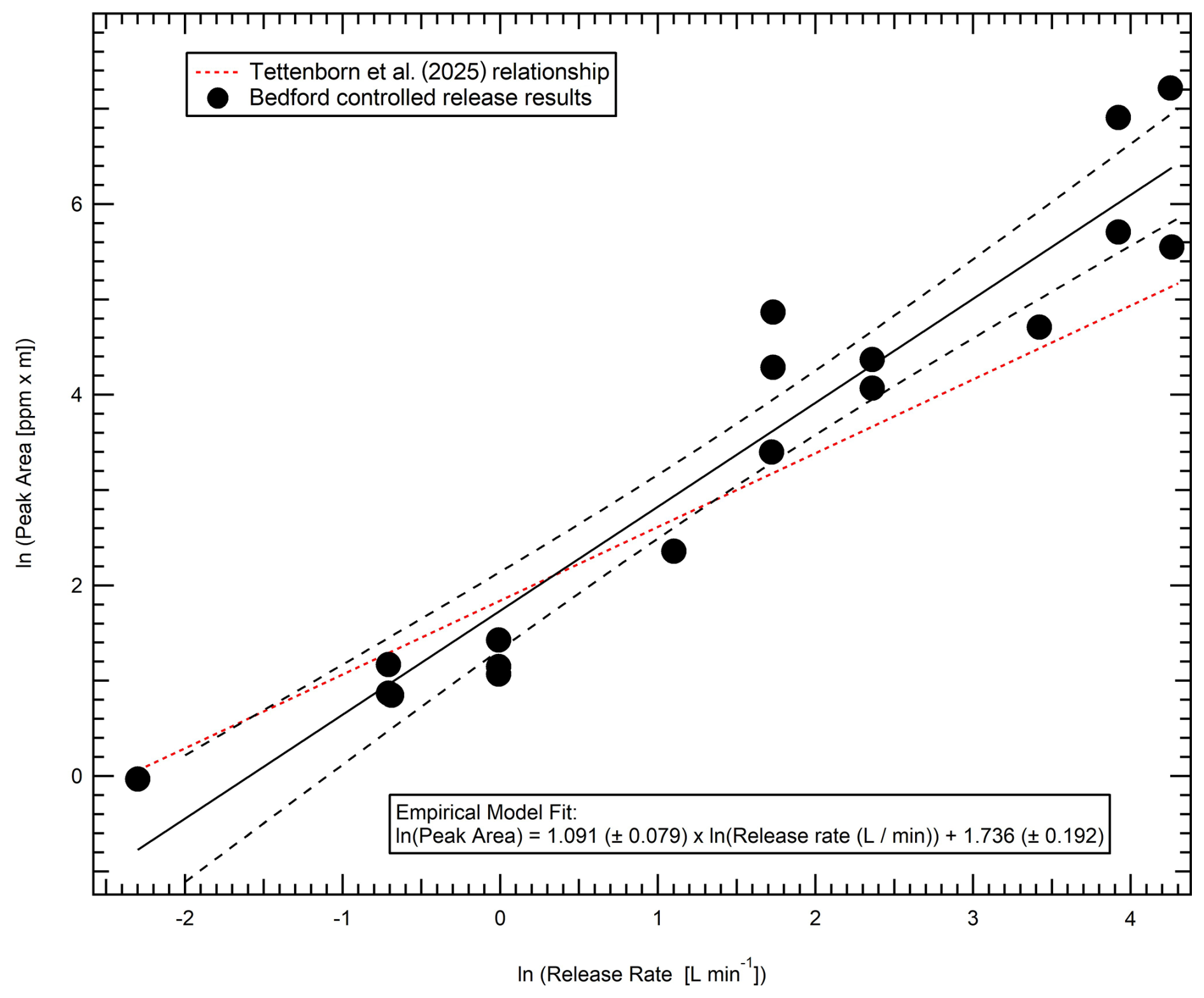
Figure 5 Peak area vs. actual release rate for plume transects within 30 m of release. Data shown is an average of multiple transects (at least 10) for each release.

In order to reduce the uncertainty for the WASP as much as possible, we present the results of a 1 week controlled release experiment conducted under variable wind conditions in a simple open field environment. Whilst this does not replicate the complex conditions of an urban setting, previous work in Tettenborn et al. (2025) shows that combined results from both urban and open field settings can be combined to give a generalised trend to create a plume area emission algorithm. For the WASP, the setup is slightly different to the work in Tettenborn et al. (2025), with the WASP's inlet located on the driver's side at low elevation. This may influence the impact of vehicle turbulence on the measurements and the difference in elevation will lead to a different vertical section of the plume being sampled. A comparison between the results of the Bedford controlled release, and the Tettenborn et al. (2025) methodology averages are shown below in Fig. 5. All data shown is for downwind transects, where the plume was intercepted at a maximum of 30 m from the controlled release location. The plume area is calculated as a function of distance travelled (as opposed to time), to correct for vehicle speed differences as done in the original Tettenborn et al. (2025) work.

Whilst the general trend of increasing plume area with release rate is adhered to, as can be seen in Fig. 5, the gradient of the trend is steeper, implying that a near-ground based inlet is potentially more capable of ascribing differences in emission rates.

One of the expected limitations of the algorithmic methods is that the effect of wind speed is ignored. Given the importance of wind speed in emissions modelling (e.g. Gaussian plume modelling from vehicles, Dowd et al., 2024), it would appear to have the potential for significant uncertainty in the resultant emissions quantification. To test this, 1 Hz wind data (averaged to 1 min data) was taken from the 3 m mast located on site at the controlled release and incorporated into the analysis according to Eq. (5).

$$\begin{array}{}\text{(5)}& \text{wind speed}\times {\int }_{\text{plume start}}^{\text{plume end}}\left[{\mathrm{CH}}_{\mathrm{4}}\right]\end{array}$$

The results of the integration of wind speed into the algorithm are shown below in Fig. 6. Possibly somewhat surprisingly, there is a slight decrease in the goodness of fit to the relationship, potentially due to plume dynamics close to source not being immediately controlled by the atmospheric conditions, but the dynamics of the emission. This may also provide evidence as to the reasons why the results of previous studies have ended up with metrics that would at first seem unlikely to be able to produce reliable results from atmospheric dispersion principles. Given this result, that it seems to be as robust to consider wind as to not, it may be prudent for future controlled release experiments to focus on recreating the conditions of gas migration prior to emission to the atmosphere to see if this result still holds true.

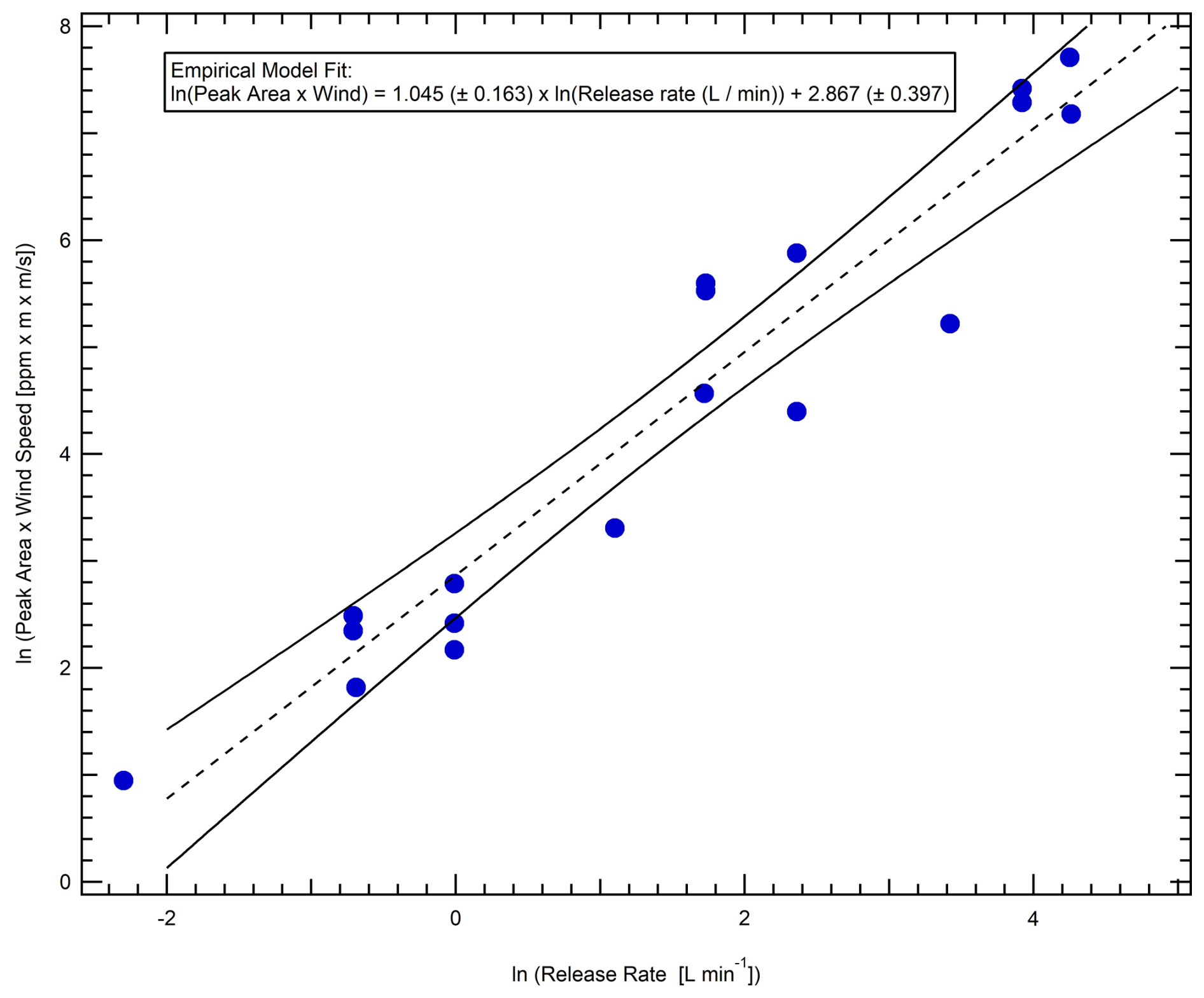
Figure 6 Peak area multiplied by wind speed vs. actual release rate for plume transects within 30 m of release. As with Fig. 5, data shown is an average of multiple transects (at least 10) for each release.

Due to these findings, the quantification equation used within York mobile surveys is shown in Eq. (6).

$$\begin{array}{}\text{(6)}& \begin{array}{rl}\ln (\text{release rate}/\mathrm{L}{\min }^{-\mathrm{1}})=& \mathrm{0.9167}\times \ln \left(\text{Peak Area}\right)\\ & -\mathrm{1.7359}\end{array}\end{array}$$

Additionally, leak rates were then reported within bins, similar to Tettenborn et al. (2025), where three possible bins were assigned; high (>40 L min⁻¹), medium (6–40 L min⁻¹) and small (<6 L min⁻¹). This was adapted for the York surveys, the small category was changed to 2–6 L min⁻¹ and a new category, very small, was introduced which contained leak rates of 0–2 L min⁻¹. This change was introduced due to the lower enhancement criteria within the York methodology which allowed for detection of much smaller fugitive emissions.

It is important to note that these results are only suitable for the specific setup utilised here and should not be more widely applied without corroboration with other instruments or platform packages.

2.4.2 Instrument Lag Time

For each of the releases, the lag time between detecting C₂H₆ and CH₄ enhancements was calculated. Due to the response times of the instruments, it was expected that the TILDAS would respond to an enhancement before the MGGA, however, this assumes that both instruments receive the same packet of air at the same time, while, in reality, the packet of air will take a different amount of time to flow through the manifold to each instrument. To determine a more accurate lag time for the instruments, the maximum CH₄ enhancement for each transect was identified along with the maximum C₂H₆ enhancement occurring within 5 s of the CH₄ enhancement. The resulting 10 s window was selected based on vehicle speeds during the controlled release, where the WASP travelled at roughly 20 mi h⁻¹. Over the course of 10 s (5 s either side of the methane maximum) this would result in a distance of 85 m covered (the average length of a transect being 180 m). The time lag between C₂H₆ and CH₄ showed that in most cases (88.1 %), maximum C₂H₆ concentration preceded maximum CH₄ concentration with a mean of 2.7 s before and a median of 3.8 s before. Observing a window of time of maximum CH₄ to 5 s before maximum CH₄ resulted in a mean lag of 3.3 s from C₂H₆ to CH₄ and a median lag of 3.9 s. This helped inform the detection algorithm to look for maximum C₂H₆ within a window only up to 5 s before the maximum CH₄. Density plots showing the time lag of maximum C₂H₆ from maximum CH₄ are shown in Fig. S2 in the Supplement for the full 10 s time window and Fig. S3 in the Supplement for up to 5 s before the time of maximum measured CH₄.

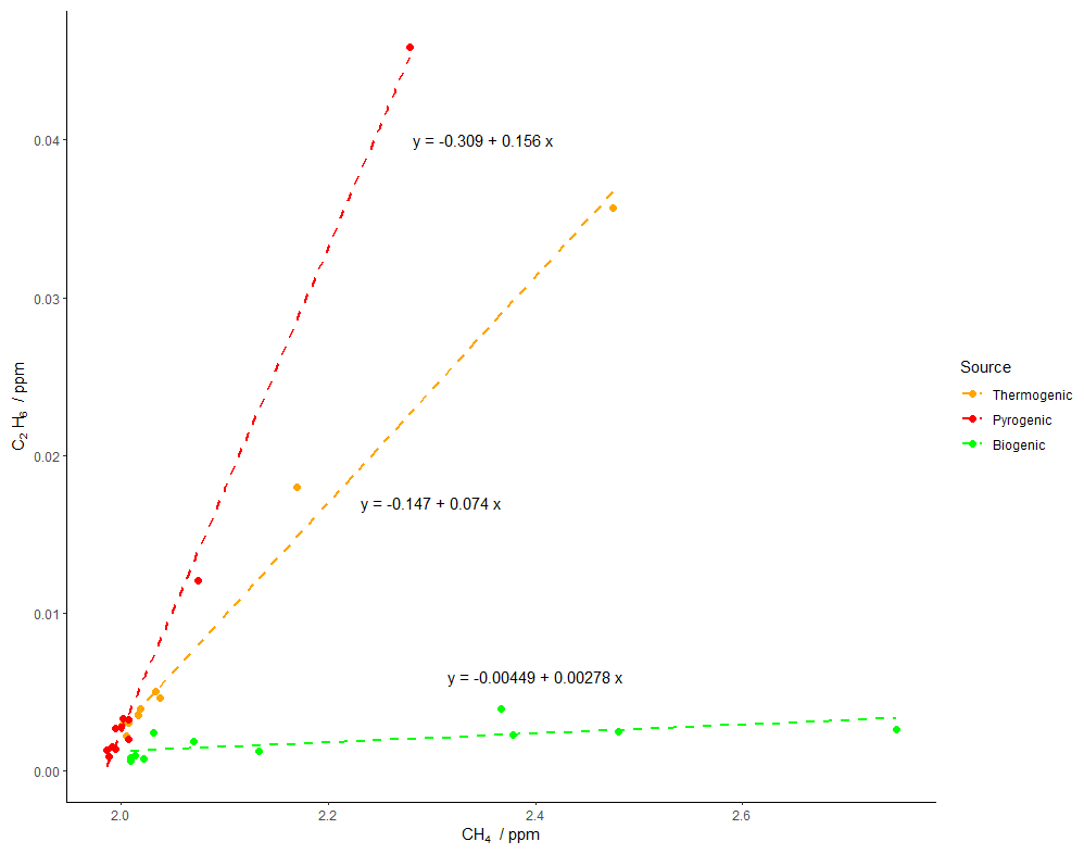
Figure 7 Relationship between CH₄ and C₂H₆ for three OPs of different source types located during the sampling campaign.

2.5 Source Appointment

Source determination using ethane : methane (C₂:C₁) ratios has been shown to be effective, due in part to the knowledge that C₂H₆ is present in measurable quantities in thermogenic gas but not biogenic gas (Fernandez et al., 2022). These ratios can be used in order to determine the source of a CH₄ emission. Demonstrated in Yacovitch et al. (2014), Lowry et al. (2020), Defratyka et al. (2021), and Fernandez et al. (2022), ${\mathrm{C}}_{\mathrm{2}}:{\mathrm{C}}_{\mathrm{1}}<\mathrm{0.005}$ may be associated with biogenic sources, >0.005 to <0.09 are thermogenic and >0.1 are considered pyrogenic or combustion. Ideal examples of these relationships are shown in Fig. 7. In order to calculate these ratios, CH₄ and C₂H₆ values must first be aligned in time, due to them being measured on separate instruments, the criterion for time alignment was discussed in Sect. 2.4.2. Additionally, enhancements are removed where the R² of CO₂:CH₄ is greater than 0.9 to ensure no combustion sources are wrongly assigned as thermogenic.

3 Results

3.1 Results of York mobile surveys

18 mobile surveys were conducted across the route of York, the raw data was taken from 10 Hz files for CH₄ (MGGA) and C₂H₆ (TILDAS) and time averaged to 1 Hz data to be of the same response time as the WASPs other internal components (e.g. GPS), a colour map of the measured CH₄ concentration is shown in Fig. 8. The data was then processed to remove measurements taken when vehicle speeds were 0 or >40 mi h⁻¹ as well as removing data within the area of WACL, as calibrations and other instrument tests were conducted in this location. A rolling 2.5 min median background of CH₄ was then applied and enhancements were determined as any CH₄ measurement taken that was greater than 1.05 times the calculated background. The enhanced readings were then clustered such that any elevated reading within one second of another were assumed to correspond to the same enhancement. These enhancements were then spatially averaged such that 468 OPs were detected over the course of the 18 mobile surveys.

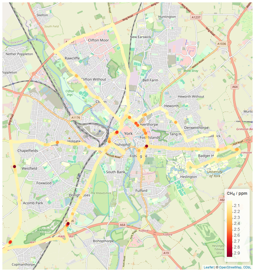
Figure 8 Colour map of CH₄ concentration from one of the York mobile surveys. Produced using Leaflet (Cheng et al., 2025) with tiles taken from OpenStreetMap (© OpenStreetMap contributors https://www.openstreetmap.org/copyright, last access: June 2026).

For each of these OPs the maximum C₂H₆ value was found from the time of maximum CH₄ to 5 s prior. The two instruments' data were then aligned for each OP such that time of maximum CH₄ measurement was equal to time of maximum C₂H₆ measurement. A linear regression was then taken of values from 5 s prior to the maximum methane measurement to 5 s after and a source type was assigned such that ${\mathrm{C}}_{\mathrm{2}}:{\mathrm{C}}_{\mathrm{1}}<\mathrm{0.005}$ is associated with biogenic sources, >0.005 to <0.09 are thermogenic and >0.1 are considered pyrogenic or combustion.

Of the 468 OPs, 177 (37.8 %) were found to be thermogenic in origin. All thermogenic OPs were then spatially clustered using a 30 m threshold, with the resulting clusters filtered to ensure that each cluster contained OPs occurring on at least two separate mobile surveys, removing any OPs occurring from an event observed during only one mobile survey. The remaining clusters were then averaged into LIs such that the latitude and longitude were calculated as a weighted spatial average, resulting in 24 thermogenic LIs from the 177 thermogenic OPs. Leak rate was determined using the equation present in Sect. 2.4.1 using the mean ln (peak area) of all OPs within each LI cluster. The smallest leak rate was determined to be 0.01 L min⁻¹ and the largest being 4.13 L min⁻¹, when assigned to bins 2 were classified as small (2–6 L min⁻¹) and 22 were very small (0–2 L min⁻¹). When the source determination step was omitted, it resulted in 58 LIs with leak rates ranging from 0.01–4.70 L min⁻¹, when assigned to bins 9 were small (2–6 L min⁻¹) and 49 were very small (0–2 L min⁻¹).

Industry applicability

As many gas distribution companies have signed up to voluntary emission reporting programmes, such as the Oil and Gas Methane Partnership (OGMP) 2.0, they are now obligated to report emissions through measurement based methods. One of the most popular methods for such a reporting programme is through comprehensive, repeated vehicle based measurement surveys of an operator's gas network. Here, we have a repeated route of measurements where thermogenic emissions have been reported at certain locations throughout the campaign. It is therefore interesting from a mitigation perspective to investigate how many times each thermogenic emission was detected over the course of the campaign.

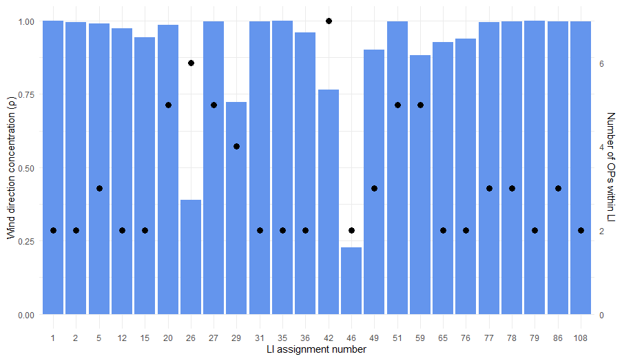
Figure 9 Wind direction consistency and number of OPs per thermogenic leak indication detected during the York campaign.

The effect of wind on detection of LIs was initially investigated by calculating the mean resultant length of wind directions when a thermogenic OP was detected. This was calculated using Eq. (7).

$$\begin{array}{}\text{(7)}& \mathit{\rho }={\displaystyle \frac{\mathrm{1}}{n}}\sqrt{{\left({\sum }_{i=\mathrm{1}}^n\cos {\mathit{\theta }}_i\right)}^{\mathrm{2}}+{\left({\sum }_{i=\mathrm{1}}^n\sin {\mathit{\theta }}_i\right)}^{\mathrm{2}}}\end{array}$$

Where:

• ρ is mean resultant length

• n is number of data points

• θ_i is the angle in radians

For this analysis ρ is close to 1 when the wind directions are concentrated (similar) and close to 0 when more dispersed. Figure 9 shows that for the majority of LIs detected in York, ρ is close to 1, suggesting that most LIs occur away from the road and require correct wind direction to be detected.

The number of mobile surveys is a large factor in the probability of detecting an LI. Each LI requires the enhancement to be detected on at least 2 separate mobile surveys. Of the 24 LIs detected over the course of this campaign, 12 LIs were detected on 2 mobile surveys, 6 were detected on 3 mobile surveys, 4 on 5 mobile surveys and 2 on 7, resulting in an average probability of detection of 0.18. Detection versus non detection for each LI is demonstrated in Fig. 10. This low probability of detection highlights the need for surveys with multiple repeats.

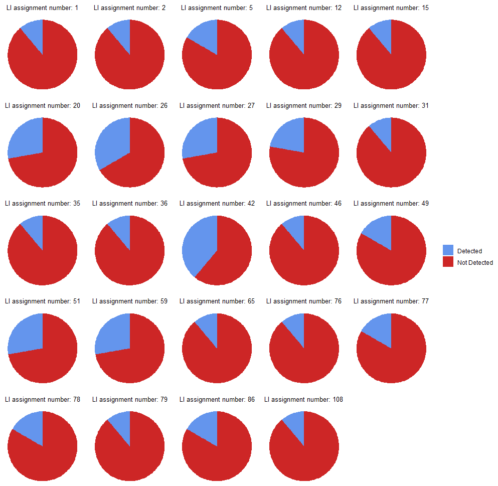
Figure 10 Pie charts of each LI detected during the York campaign showing detection frequency of its respective OPs.

3.2 Emissions from other sources

While 177 of the 468 OPs were determined to be thermogenic, 39 were assigned as biogenic (8.3 %), 199 were pyrogenic (41.8 %) and 53 were not able to be assigned a source type. NO_x:CO₂ ratios were investigated for the pyrogenic OPs using the same methodology used for C₂:C₁ source assignment. 115 of the 199 pyrogenic OPs were able to be analysed in this way, 87 of these 115 OPs (75.7 %) had a NO_x:CO₂ ratio $<\mathrm{0.88}\times {\mathrm{10}}^{-\mathrm{3}}$. This implied that the majority of pyrogenic emissions did not originate from traffic, but were more likely emissions from domestic heat and power generation (such as emissions from domestic boilers, Cliff et al., 2025).

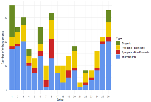
Emissions from pyrogenic and biogenic sources were compared to thermogenic emissions at the OP stage on a mobile survey by mobile survey basis due to the high unlikelihood of pyrogenics and biogenics being persistent emission sources, the number of times each source type was detected per mobile survey is shown in Fig. 11.

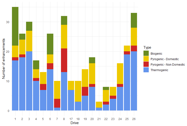
Figure 11 Total number of enhancements from each source type detected during each mobile survey of the York campaign.

Thermogenics were the most frequently located source type on 13 of the 18 surveys, with mobile surveys 7, 18, 19, 21 and 22, finding pyrogenic emissions related to heating and cooking were the most frequently occurring source type.

3.3 Comparison to previous methods

The main alterations to this methodology from that presented in Weller et al. (2019) (and other studies that were based off this method) was the decrease in enhancement criteria from 1.1 times the baseline to 1.05 times the baseline, a decrease in the clustering time window from 5–1 s and the addition of a source determination stage as a core step in the algorithm, as opposed to previous iterations that either had no source determination stage, or one that came later in the analysis. Table 1 shows the effect of each of these changes on the resulting detection of OPs and LIs.

Table 1 Number of detected OPs and LIs depending on algorithm parameters.

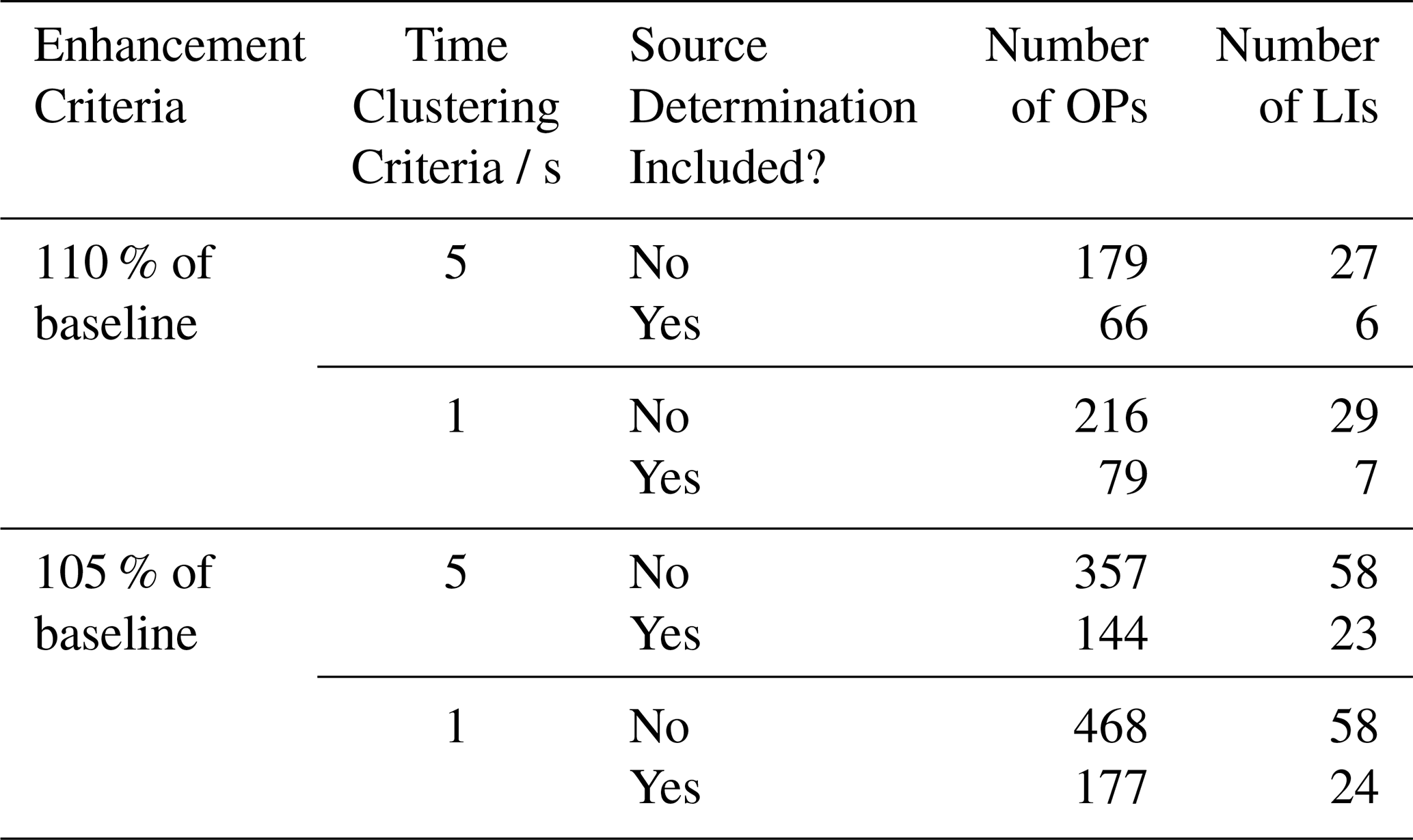
These results show the new methodology could locate more LIs. Binning into the leak rate categories of very small (0–2 L min⁻¹), small (2–6 L min⁻¹), medium (6–40 L min⁻¹) and high (>40 L min⁻¹) showed that of the 24 LIs in the new source filtered methodology, 2 were small and 22 were very small. For the 58 LIs of the new non filtered methodology, 9 were small and 49 were very small. For the 27 LIs detected in the original unaltered methodology 10 were small and 17 were very small. Finally, for the 6 LIs detected when applying the source determination step to the original unaltered methodology, 1 was small and 5 were very small. This shows the original methodology, requiring an enhancement of 1.1 times the baseline with 5 s time clustering, misses a large proportion of LIs that the newer methodology, requiring an enhancement of 1.05 times the baseline with 1 s time clustering, detects. A large proportion of these missed LIs occur in the very small category as expected with a smaller enhancement criteria. Source filtering shows that regardless of criteria used, less LIs will be detected with this included in the method. This suggests previous methodologies that do not use this stage may be mischaracterising some thermogenic enhancements as being permanent, as they may instead be detecting methane enhancements of differing source types that occur within the same vicinity of one another.

3.4 Comparison of alternate quantification approaches

As previously described, the quantification equation used within this body of work is based on the Tettenborn et al. (2025) approach of using peak area to calculate the leak rate of LIs. However, previous works have used the quantification equation present in Weller et al. (2019) which quantifies release rate based on peak height. This campaign's results were reprocessed using each of these previous quantification equations in order to compare the effects of the updated parameters in the York quantification equation to the original, present in Tettenborn et al. (2025) but also to explore the difference in quantified leak rates from a peak height approach. As previously mentioned, the results of the York quantification approach resulted in the 24 LIs being assigned to leak rate bins such that 2 were small and 22 were very small, the Tettenborn et al. (2025) equation results in 1 medium, 1 small and 22 very small and the Weller et al. (2019) equation results in 1 small and 23 very small. The specific leak rates of LIs calculated with these three equations are presented in box-plots in Fig. 12.

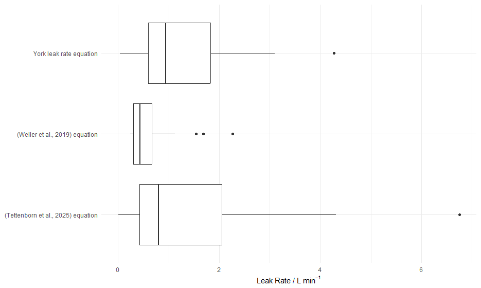
Figure 12 Comparison of calculated leak rates of LIs detected during the York campaign, using each of the 3 quantification equations previously discussed.

This shows that both the peak area approaches result in a much larger range of calculated leak rates from the LIs than from the peak height approach present in Weller et al. (2019). This suggests that the instrumentation used to detect CH₄ enhancements may result in low, wide peaks as opposed to higher, sharper peaks, thus explaining why leak rates are weighted much lower from this method. The Tettenborn et al. (2025) equation appears to be mostly consistent with the equation determined from the York methodology, however there is slightly higher weighting of leak rates with the Tettenborn et al. (2025) equation, resulting in the 24 LIs changing from the assignments of 5 small and 19 very small to 1 medium, 5 small and 18 very small.

4 Conclusions

This study focused on using the limitations of instrumentation to better inform a detection algorithm. Enhancement criteria was determined by investigating the variance of the MGGA, although laboratory experiments suggested the instrumentation was capable of detecting enhancements at a minimum of 1.005 times the baseline, in-field experiments showed that an enhancement criteria of 1.01 times the baseline was more likely the lower limit for detection. However, for the surveys a criteria of 1.05 times the background was selected so as to not incorporate small, diffuse emissions within the analysis. Response rate of the instruments was calculated to inform the time window for clustering, with both MGGA and TILDAS having sub 1 s response rate, the time clustering was limited to 1 s due to the limitations of GPS data collection speed. Employing the parameters used in previous methodologies, resulted in the detection of 27 LIs compared to the 58 LIs detected using updated parameters (53.5 % less), the parameter change has also shown the ability to detect more LIs in all leak rate categories, but in particular, the very small (0–2 L min⁻¹) category, where 17 of 27 LIs were located in the previous methodology, but 46 of the 58 were located in the new methodology.

Source determination proved to be a useful tool for predicting emissions directly related to natural gas, when source filtering was introduced at the OP stage of detection, it resulted in only 41.4 % of LIs still being detected as opposed to the non-source filtered method.

Additionally, source determination has helped to highlight that although thermogenic emissions from natural gas are the highest contributor to CH₄ emissions, pyrogenic emissions related to domestic heat and power generation also provide a high, but often overlooked contribution to a city's CH₄ emissions.

Updating the quantification equation from a peak height approach to a peak area approach resulted in a much wider range of leak rates being calculated in the study. However, these values were not as high as when quantified using the original equation presented in Tettenborn et al. (2025).

This new method has shown that by changing enhancement criteria and time clustering parameters, it is possible to detect many more LIs, but that by applying a source determination step at the OP detection stage there is a reduction in the number of detected LIs due to the reduction in the incorrect assignment of OPs. However, the methodology has the ability to improve further, primarily by employing instrumentation that is capable of detecting both CH₄ and C₂H₆ so as to remove uncertainty related to time lag between two instruments. Secondly, improvement can be made by having all instrumentation and hardware able to operate at a sub 1 s response rate in order to reduce the time clustering parameter limit and further improve spatial resolution.