Classification of atmospheric aerosols over Urmia Lake based on lidar observations

This study provides new observational evidence on the contribution of salt-dust plumes originating from the desiccated bed of Urmia Lake. The near-surface atmosphere over the lake bed was investigated using a scanning polarization lidar. Nighttime measurements at 532 nm were conducted in September 2022, with the instrument operating in azimuthal scan mode. Investigations show that the aerosol plumes above the lake contain both dust and salt particles. A modified two-step polarization-lidar photometer networking retrieval scheme was applied to lidar azimuthal scans to obtain backscatter ratios and mass concentrations of dust, salt-dust, and wet-salt aerosols. Plume regions were detected and isolated from their surroundings using a multi-scale layer detection algorithm. Averages of particle linear depolarization ratios, backscattering coefficients, and mass concentrations for each detected plume are retrieved to quantify the contributions of different particle types to the plume composition. The retrievals indicate that salty particles exhibit characteristically lower linear depolarization ratios but substantially higher backscattering than pure dust particles. The results demonstrate that even relatively low mass fractions of saline aerosols markedly enhance particle backscattering over the dried lake bed. Based on plume-averaged backscattering values, the detected aerosol plumes were classified as dust-dominant, salt-dominant, or mixed mode. Analysis of 64 individual plumes revealed that 47 % of them were salt-dominant, 25 % dust-dominant, and 28 % in mixed mode.

1 Introduction

The drying of lakes and their transformation into sources of dust and atmospheric particles are environmental disasters, with well-known examples including Lake Chad, Aral Sea, Great Salt Lake, and Urmia Lake (Evans et al., 2004; Indoitu et al., 2015; Skiles et al., 2018; AghaKouchak et al., 2015). Such areas often become significant sources of aerosols, affecting the air quality, climate, ecosystems, and human health.

Urmia Lake, an endorheic hypersaline lake in Northwest Iran (Fig. 1), has long hosted unique ecological communities, including Artemia Urmiana and migratory birds (Eimanifar and Mohebbi, 2007). However, since the mid-1990s, the lake has suffered severe desiccation due to both climate variability and extensive water mismanagement (Garousi et al., 2013; Abbaspour et al., 2012; Delju et al., 2013; Schulz et al., 2020; Hassanzadeh et al., 2012; AghaKouchak et al., 2015; Taravat et al., 2016; Schmidt et al., 2021). The shrinking water body has exposed vast areas of salt flats, which act as new sources of saline dust (Ahmady-Birgani et al., 2020; Boroughani et al., 2019), degrading air quality, and threatening regional health and livelihoods (Ghale et al., 2021).

Different satellite-, model-, and ground-based studies have examined the atmospheric aerosols over the Urmia Lake. The studies emphasize the impact of salt aerosols on the atmosphere. Ahrari et al. (2024) studied six shrinking lakes across the Iranian Plateau, including Urmia Lake. They showed that, following an 81 % reduction in lake area, dust storm frequency increased by around 20 %, confirming the strong link between lake desiccation and dust storms (Ahrari et al., 2024). Gholampour et al. (2015) investigated the composition of atmospheric particles around Urmia Lake and identified their origins from both natural and anthropogenic sources. In 2013, aerosol samples collected at two coastal sites showed water-soluble ions accounted for approximately 11 %–13 % of the total suspended particles mass. A two-year Calitoo sun-photometer campaign (November 2020–October 2022) near the lake revealed that fine urban-industrial aerosols predominated in winter, whereas coarse particles were more prevalent in summer. Of the 538 measurement days, approximately 69 % were classified as urban-industrial, about 10 % as dust, and around 20 % as mixed aerosols that most probably contain salt too (Alizadeh et al., 2024a). Mardi et al. (2018) analyzed Aerosol Optical Depth (AOD) data recorded by the Moderate Resolution Imaging Spectroradiometer (MODIS, onboard Terra and Aqua satellites) from 2001 to 2015. They stated that despite ongoing desiccation of the lake, salt emissions from the lake surface are not the primary drivers of the AOD increase in the region. In fact, trans-regional dust significantly contributes to the aerosol content of the lake atmosphere. Ghomashi and Khalesifard (2020) analyzed a decade of aerosol patterns in the Urmia Lake region (June 2006–December 2017) using satellite observations. The study incorporated MODIS AOD measurements and vertical aerosol profiles from the Cloud-Aerosol Lidar with Orthogonal Polarization (CALIOP), onboard Cloud-Aerosol Lidar and Infrared Pathfinder Satellite Observations (CALIPSO) satellite. They reported that the lake serves as a local aerosol source during the driest months of the year (June–September). Additionally, they discovered that large neighboring dust sources, such as the Mesopotamian region, have a stronger influence on the area than the lake itself. Hamzehpour et al. (2022) found that the mineralogical and elemental compositions of soil and airborne dust samples were strongly linked. This indicates that the identified playa soils are indeed sources of regional dust.

Despite these advances, distinguishing between mineral dust, salt-dust i.e., a mixture of salt and mineral dust, and anthropogenic aerosols over the Urmia Lake remains challenging. CALIOP algorithms often misclassify salt particles as polluted dust subtype, and near-surface aerosol layers are not well resolved (Ghomashi and Khalesifard, 2020). Ground-based aerosol lidars offer unique opportunities to overcome these limitations by providing high-resolution profiling of aerosols' physical and optical properties, thereby enabling more accurate classification of local salt dust versus transported mineral dust. The particle linear depolarization ratio (δ_p) and lidar ratio (S) are key parameters in lidar data analysis (Freudenthaler et al., 2009; Tesche et al., 2009; Burton et al., 2012; Hofer et al., 2020; Floutsi et al., 2023). The δ_p is primarily dependent on particle shape, whereas the S defined as the extinction-to-backscatter ratio is more closely related to particle type. Both coefficients vary with environmental conditions such as relative humidity (RH). Haarig et al. (2017) reported that at low RH (∼40 %), δ_p and S for salt particles at 532 nm are approximately 0.15±0.03 and 25±3 sr, respectively. At higher RH (RH >80 %), these values decrease to about 0.03±0.02 and 23±2 sr. There are slight differences in the reported values of particle linear depolarization and lidar ratios for dust particles, depending on their origins. Floutsi et al. (2023), in a valuable work, collected different lidar-derived optical properties of atmospheric aerosols originating from different sources. They found a considerable similarity between the Central Asian and Middle Eastern dust, where δ_p and the lidar ratio S at 532 nm vary in the range of 26.8 %–33.2 % and 35–43 sr, respectively. For the Saharan dust, the former is in the range of 26.7 %–29.3 % and the latter in 45–61 sr. These distinct behaviors make δ_p and S effective parameters to distinguish between salt and dust particles using lidars in marine environments. Hofer et al. (2020) conducted multiwavelength polarization Raman lidar measurements in Dushanbe, Tajikistan, from March 2015 to August 2016. For 15 % of the 276 cases, they detected layers that most probably contained dry salt, or particles formed of dust and salt mixtures. They mentioned that such particles may be raised from the dried lakes or saline playas in the region. For lidar measurements at 532 nm, they reported very low extinction coefficients ($<\mathrm{30}{\mathrm{Mm}}^{-\mathrm{1}}$), S<25 sr, and δ_p ∼0.15–0.20, for such layers.

We installed a scanning polarization lidar operating just at 532 nm at the southwestern coast of Urmia Lake from September 2018 to October 2022. Therefore, all reported parameters in this analysis and cited papers, including the linear depolarization ratios (δ), lidar ratios (S), and backscattering coefficients (β), refer to values for 532 nm; unless otherwise, the corresponding wavelength is indicated. The Lidar capability to operate in both azimuthal and zenith modes enables monitoring of both local and trans-regional aerosols over Urmia Lake (Khalesifard et al., 2020). In our previous research, we employed ground-based polarization lidar to investigate the vertical distribution of atmospheric particles over Urmia Lake. From July to October 2020 and 2021, some dust plumes with ${\mathit{\delta }}_{\mathrm{p}}=\mathrm{0.23}\pm \mathrm{0.05}$ were observed that originated from the Middle Eastern sources. 20 of them were from Mesopotamia, which were observed at the altitude ranges of 2.50±0.85 km above ground level (a.g.l.), and a single one that rose up from the Arabian desert was detected at 0.90±0.20 km a.g.l. (Alizadeh et al., 2022). In October 2021, one notable case involved a lofted dust plume (${\mathit{\delta }}_{\mathrm{p}}=\mathrm{0.21}\pm \mathrm{0.02}$) from Niger, Africa, detected in Urmia Lake atmosphere at ∼8 km a.g.l. after about 140 h of transport (Alizadeh et al., 2024b). From November 2021 to February 2022, the type of atmospheric particles undergoes marked changes. Lidar measurements indicated that the lower atmosphere near the lake surface is dominated by anthropogenic aerosols, with lower δ_p values of <0.10. The densely populated and industrialized catchment area surrounding Urmia Lake significantly contributes to elevated levels of anthropogenic aerosols during the winter months (Alizadeh et al., 2022).

In this study, we used the horizontal-scanning polarization lidar, operating at 532 nm, to investigate near-surface aerosol layers over the desiccated bed of Urmia Lake during summer. A layer detection algorithm was applied to isolate the plume from the background atmosphere (Mao et al., 2011). For each plume, we retrieved the particle backscatter coefficient (β_p) using the well-known technique introduced by Klett (1981, 1985); Fernald (1984), and following the approach introduced by Biele et al. (2000) and used by many other teams, e.g., Freudenthaler et al. (2009); Tesche et al. (2009), we obtained the δ_p values for different lidar recordings. We modified the two-step POlarization-LIdar PHOtometer Networking (POLIPHON) method (Mamouri and Ansmann, 2014, 2017) to process these parameters and classify the aerosols into three categories: dust, salt-dust, and wet-salt, and finally derived mass concentrations for these categories using appropriate characteristic lidar ratios and conversion factors (Ansmann et al., 2011, 2012).

The remainder of this paper is organized as follows: Sect. 2 describes the instrumentation and methodology. Section 3 covers the results of the analyses and discusses the findings, and Sect. 4 includes the summary and conclusions of the work.

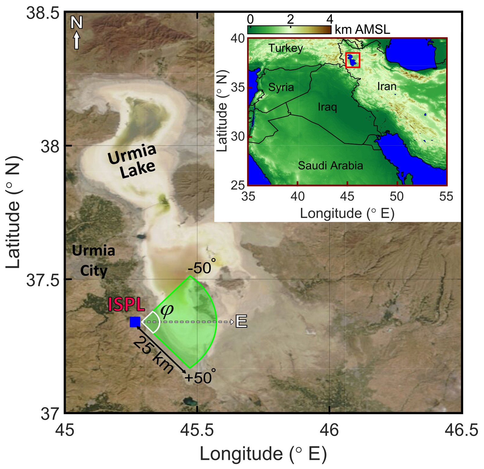
Figure 1 Urmia Lake in Northwest Iran, Terra MODIS true color, 20 September 2022. The blue square on the lake coast is the ISPL station at 37.34° N, 45.29° E, and 1270 m a.m.s.l. The green-shaded area represents the lidar azimuthal coverage over the lake. Inset is the topography map of the region. Terra/MODIS imagery courtesy of NASA LAADS DAAC.

2 Instrumentation and methodology

This section provides details of the polarization lidar setup and the technique utilized in this work to monitor and classify atmospheric particles over the lake.

2.1 IASBS scanning polarization lidar

The IASBS scanning polarization lidar (ISPL) is a single-wavelength (532 nm) linear polarization lidar that is designed and constructed at the Institute for Advanced Studies in Basic Sciences (IASBS) remote sensing laboratory. The ISPL is installed on the southwest coast of Urmia Lake, at 37.34° N, 45.29° E, and 1270 m above mean sea level (a.m.s.l.) (see Fig. 1). The system operates in two modes: zenith-aiming or horizontal azimuthal scanning (Khalesifard et al., 2020). For this study, horizontally scanned data were used. The ISPL transmitter consists of a frequency-doubled, 10 ns pulsed Nd-YAG laser and a 10× beam expander. The output energy per pulse at 532 nm is approximately 100 mJ at a repetition rate of 2 Hz. The full overlap range of the ISPL is at a distance of ∼3.0 km from the lidar. On the receiver side, a Cassegrain telescope with an 8-inch primary mirror and focal length of 1950 mm collects the backscattered light. Signals at 532 nm are recorded in both parallel and perpendicular polarization channels relative to the transmitted pulse. Data acquisition is performed using a four-channel, 350 MHz Tektronix digital oscilloscope. The system performs azimuthal scanning from $\mathit{\phi }=-\mathrm{50}$ to +50°, where φ=0° corresponds to the east direction in Fig. 1. Azimuthal scans performed in steps of 0.1° of the arc (Khalesifard et al., 2020). Further details on the ISPL optical setup can be found in Panahifar et al. (2020). Each complete azimuthal scan takes ∼45 min. To minimize background noise, all lidar measurements are conducted during the night (see Fig. 2).

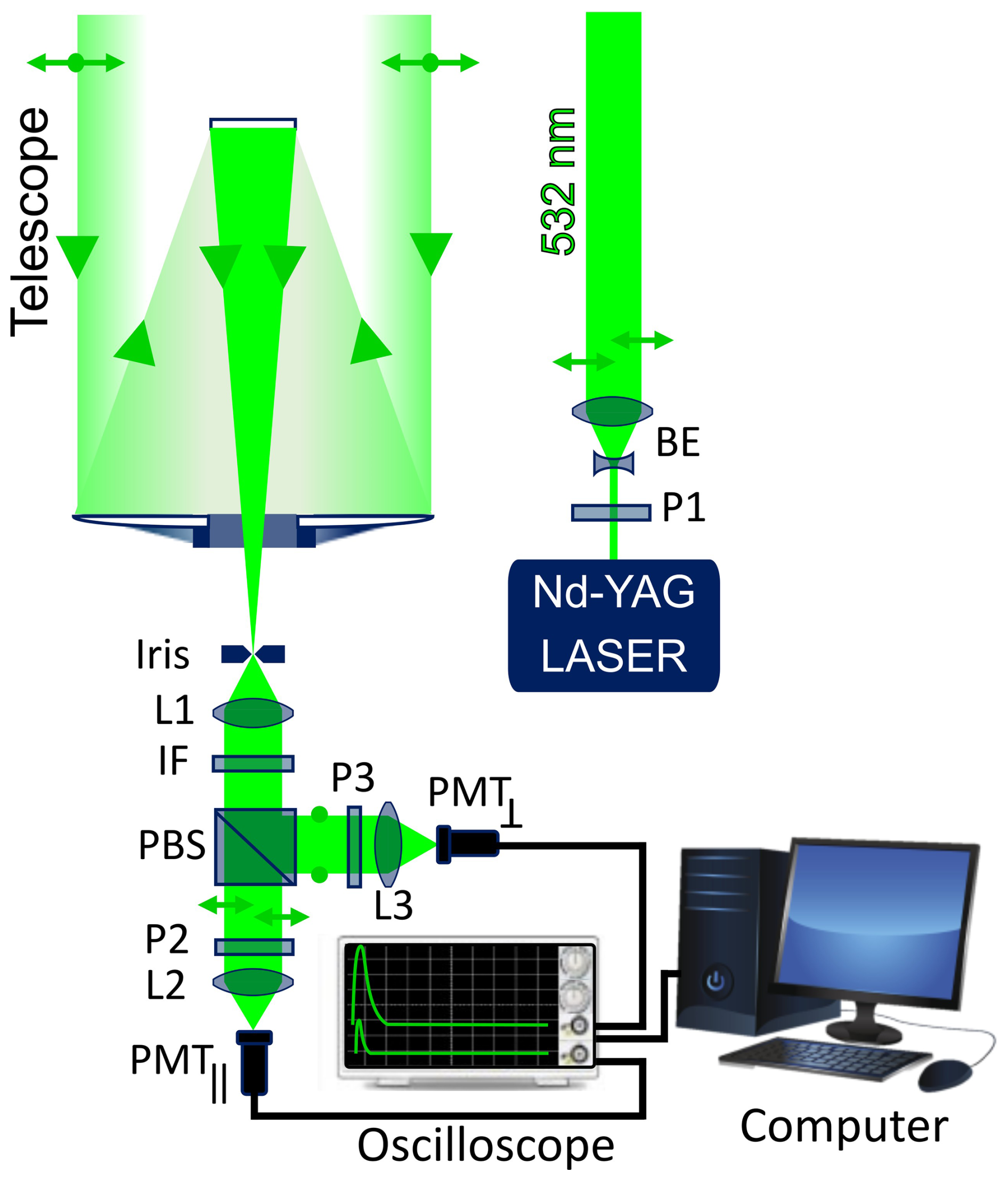
Figure 2 The ISPL optical setup: P-polarizer, BE-beam expander, L-lens, PMT-photomultiplier tube, PBS-polarizing beam splitter, IF-interference filter.

2.2 Initial processing: particle backscatter coefficient and linear depolarization ratio

Using polarization lidar recordings, key aerosol parameters can be derived, including the backscattering coefficient and the linear depolarization ratio. These parameters are essential for particle classification (Freudenthaler et al., 2009; Tesche et al., 2009; Burton et al., 2012; Groß et al., 2013; Kim et al., 2018; Hofer et al., 2020; Wandinger et al., 2023; Floutsi et al., 2023, 2024). The well-known Klett-Fernald algorithm (Klett, 1981; Fernald, 1984; Klett, 1985) has been used to retrieve the particle backscatter coefficient, β_p. To apply this technique, a reference extinction coefficient (α_ref) is required for each recorded lidar signal. The slope method is commonly used to determine α_ref when the lidar is operating horizontally (Kovalev and Eichinger, 2004). But when aerosol plumes are present within the lidar operating range, especially when they spread over the sampling region, the technique incurs considerable errors due to difficulty distinguishing the plume from the background in the lidar signals. Shin et al. (2024) modified the slope method by dividing the lidar signal into multi-sections and investigating the statistics of the slopes of fitted lines to each section. As a result, they found an α_ref that, to a good extent, is not affected by noise and aerosol emissions. They called the technique the multi-section method (MSM), and we used it to retrieve a proper α_ref for each recorded azimuthal lidar signal. The obtained α_ref is fed into the Klett-Fernald algorithm to obtain β_p for each lidar signal. In retrieving the β_p, the aerosol lidar ratio is taken as 32 sr, which is the average value of that of dust, salt-dust, and wet salt (see Table 1). Once β_p is determined, the particle linear depolarization ratio can be calculated from the method introduced by Tesche et al. (2009).

$$\begin{array}{}\text{(1)}& {\mathit{\delta }}_{\mathrm{p}}={\displaystyle \frac{{\mathit{\beta }}_{\mathrm{m}}({\mathit{\delta }}_{\mathrm{v}}-{\mathit{\delta }}_{\mathrm{m}})+{\mathit{\beta }}_{\mathrm{p}}{\mathit{\delta }}_{\mathrm{v}}(\mathrm{1}+{\mathit{\delta }}_{\mathrm{m}})}{{\mathit{\beta }}_{\mathrm{m}}({\mathit{\delta }}_{\mathrm{m}}-{\mathit{\delta }}_{\mathrm{v}})+{\mathit{\beta }}_{\mathrm{p}}(\mathrm{1}+{\mathit{\delta }}_{\mathrm{m}})}},\end{array}$$

where the subscripts p and m refer to particle and molecular components, respectively. δ_v is the volume linear depolarization ratio (i.e., the combined depolarization of molecules and particles), and the molecular depolarization ratio is taken as δ_m=0.0036. Even though δ_m is a theoretical value, considering 1 nm bandwidth of the 532 nm interference filter (IF) in the ISPL setup and the operation temperature of the lidar (∼20 °C), it is very close with δ_m≃0.0042 reported by Behrendt and Nakamura (2002). Such a small difference in δ_m affects the retrieved δ_p (for the ISPL horizontal scans), in orders of $\mathrm{1.0}\times {\mathrm{10}}^{-\mathrm{3}}$, which is too small to affect the other retrieved parameters.

It should be mentioned that the lidar polarization channels are calibrated by the technique introduced by Freudenthaler et al. (2009). There is a subtle point on the impacts of different optical elements of the ISPL on the polarization state of the passing lights through them and eventually their effects on the measured volume depolarization. The beam expander in the transmitter part of the ISPL should be investigated for such effects. Freudenthaler (2016), in a valuable work, presented the details of such effects on the measured volume depolarization in a lidar system. We used the framework introduced by Freudenthaler (2016) and simulated the passage of a linearly polarized 532 nm laser light through the 10× ISPL beam expander in Zemax. In result, we found that the total amount of depolarization of the light after its passage through the beam expander was just $\sim \mathrm{2.3}\times {\mathrm{10}}^{-\mathrm{5}}\mathit{\%}$. Such small values of depolarization can be neglected quite easily, and we may neglect the depolarization effects of the beam expander.

Now β_p and δ_p can be fed into the POLIPHON algorithm to classify the particles (Mamouri and Ansmann, 2014).

2.3 Classification algorithm: two-step POLIPHON

Mamouri and Ansmann (2014) introduced the two-step POLIPHON method for classifying atmospheric particles into coarse dust, fine dust, and non-dust particles. Since the ISPL lidar is installed just at the lake's coast and scans the atmosphere azimuthally a few tens of meters above the lake bed, it is reasonable to consider that the atmospheric aerosols are either dust (d), salt-dust (sd), or wet-salt (ws). To classify atmospheric particles into these three types, the POLIPHON method should be modified. Figure 3 is a schematic diagram of the modified two-step POLIPHON algorithm for categorization of d, sd, and ws particles. In this algorithm, δ and β denote the linear depolarization ratio and the backscattering coefficient, respectively, while the subscript p refers to particles. β_p is obtained from the Klett-Fernald algorithm (Klett, 1981, 1985; Fernald, 1984) and δ_p driven by the method introduced by Tesche et al. (2009). The POLIPHON algorithm is sensitive to the presumed boundaries on particle linear depolarization. As Fig. 4 shows, in the first step of the algorithm, when δ_p rises beyond 0.31 (Freudenthaler et al., 2009; Mamouri and Ansmann, 2014), particles are considered as pure dust. Knowing that the depolarization ratio of dry salt particles is $\sim \mathrm{0.15}\pm \mathrm{0.03}$ (Haarig et al., 2017), and for dusty mix or polluted dust, δ_p is mainly greater than 0.12 (Burton et al., 2012). Then, on the particle depolarization line, ${\mathit{\delta }}_{\mathrm{ws}+\mathrm{sd},\mathrm{e}}=\mathrm{0.12}$ is defined as a boundary between the mixture of ws + sd particles and the region that includes all particle types (Fig. 4). Outputs of the first step of the algorithm are β_d and β_ws+sd. After that, the algorithm goes to its second step. In this step, first, the depolarization ratio of the mixture (δ_ws+sd) is retrieved. Then, it is considered if ${\mathit{\delta }}_{\mathrm{ws}+\mathrm{sd}}\le \mathrm{0.05}$, particles are just wet-salt (Haarig et al., 2017) (Fig. 4), otherwise they are a mixture of wet-salt and salt-dust particles, and their backscatter coefficients (β_ws and β_sd) are obtained from the last stage of step 2 (Fig. 3).

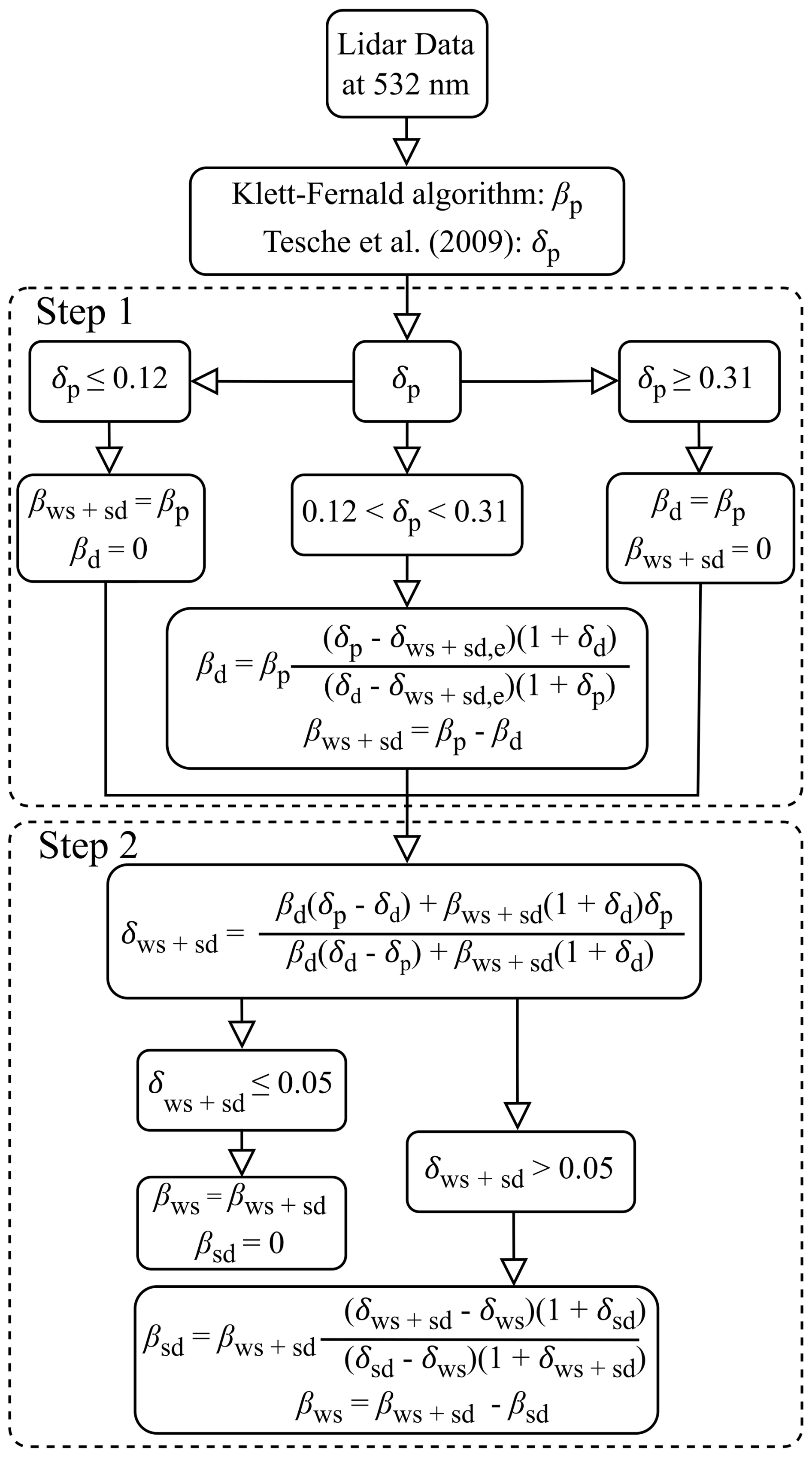
Figure 3 Modified two-step POLIPHON algorithm to retrieve backscatter ratios of dust (β_d), salt-dust (β_sd), and wet-salt (β_ws), respectively.

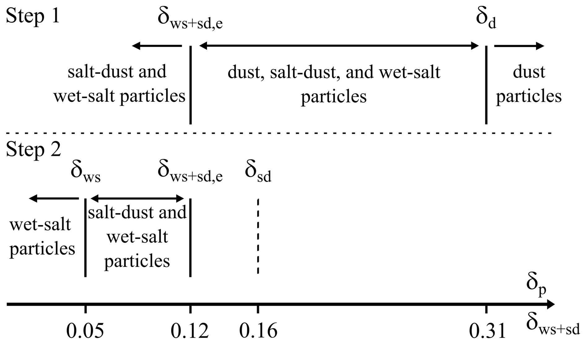
Figure 4 The depolarization ratio thresholds, used in the modified two-step POLIPHON method, are applied to distinguish wet-salt, salt-dust, and dust particles.

Hess et al. (1998)Mamouri and Ansmann (2017)Nisantzi et al. (2015)Mamouri and Ansmann (2017)Haarig et al. (2017)

Table 1 Input parameters for the conversion of particles' backscatter coefficient at 532 nm to the mass concentration based on Eq. (2).

Having β values for different types of particles, their mass concentrations, MC_i, can be obtained from Eq. (2) (Ansmann et al., 2011, 2012).

$$\begin{array}{}\text{(2)}& {\mathrm{MC}}_i={\mathit{\rho }}_i{c}_{v,i}{\mathit{\beta }}_i{S}_i,\end{array}$$

where i denotes the particle type (i.e., d, sd, and ws). The parameters ρ_i, c_v,i, and S_i represent the particle density, the extinction-to-volume conversion factor, and the lidar ratio of the corresponding particle type, respectively (Hess et al., 1998; Mamouri and Ansmann, 2017; Nisantzi et al., 2015; Haarig et al., 2017). The values of these parameters are presented in Table 1. It should be mentioned that we put the parameters ρ_i and c_v,i of the wet-salt particles similar to the marine particles in Table 1. On the other hand, since the composition of salt-dust particles isn't well known, we considered that ρ_i, c_v,i, and S_i parameters for these particles should be something between those of wet-salt and dust particles.

2.4 Layer detection: simple multiscale algorithm

Since we are making measurements just above the lake, we would like to know about the contributions of different types of particles inside a detected plume. Therefore, a plume detection algorithm should be applied to recordings of the lidar azimuthal scans. Several algorithms have been proposed for cloud- or aerosol-layer detection (Gong et al., 2011; Mao et al., 2011, 2013, 2015; Weekley et al., 2016). Mao et al. (2011) introduced a multiscale detection (MSD) algorithm to identify cloud and aerosol layers. Their method was originally designed to detect cloud boundaries where the lidar measures in the zenith direction. The method also works for dense aerosol layers. Here, we applied this method to the ISPL azimuthal scans to detect lofted plumes over the Urmia Lake dried bed. Figure 5 is a schematic range-corrected lidar signal (RCS) which also includes an aerosol layer (the red region).

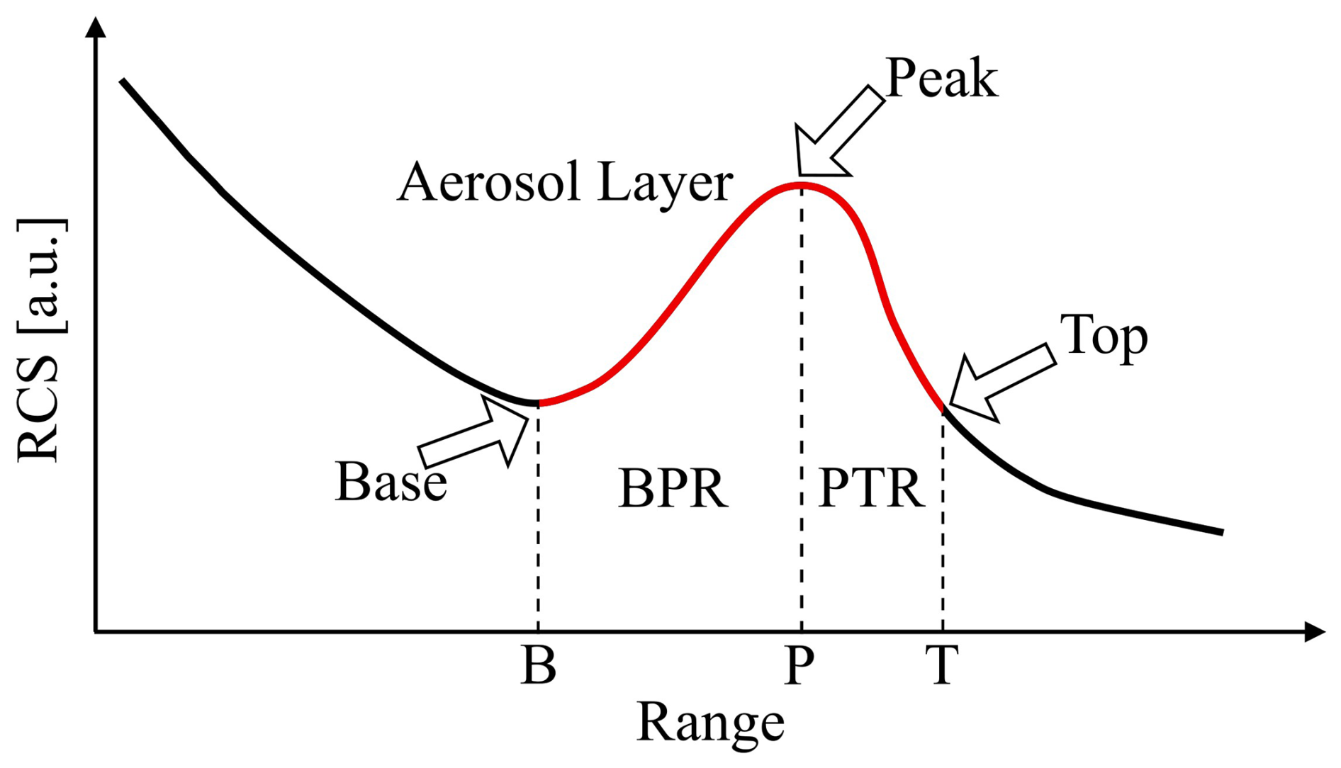
Figure 5 A schematic range-corrected lidar signal where an aerosol layer is in range, the aerosol layer can be divided into two regions: base-to-peak region (BPR) and peak-to-top region (PTR).

In the MSD algorithm, the layer has three characteristic points: base (B), peak (P), and top (T). The layer is divided into two parts: base-to-peak region (BPR) and peak-to-top region (PTR). Once the BPR and PTR are identified, the rest of the recorded data can be masked out, allowing one to deal only with the aerosol layer. To identify the aerosol layer, four steps should be followed in the MSD algorithm: (1) determining the trend index function, (2) multiscale detection, (3) overdetection rejection, and (4) base, peak, and top detection. In the first two steps, BPRs are identified using the slope sign of the range-corrected signal. The slope sign at different points of the RCS is determined by sliding windows of various sizes along the signal. Larger windows characterize the overall behavior of the signal, but smaller ones are needed to obtain information about finer features of the signal. In aerosol-free regions dominated by Rayleigh scattering, the RCS slope is generally negative. A positive slope indicates the presence of an aerosol layer and corresponds to a BPR, where the first bin can be taken as the base and the last bin as the peak of the detected layer. The third step removes spurious detections: if the difference between base and peak in the raw lidar signal is below a pre-assumed threshold, the BPR is discarded. The threshold is assumed as six times the standard deviation of the signal's far-end (tail) region. In the final step, the top of each layer is determined as the first range beyond the peak where the RCS value falls below that of the base. The range between the base and top is called the base-to-top region (BTR). After computing the BTR, the aerosol layer can be masked from its surroundings. For each detected plume in all azimuthal lidar recording profiles, we construct a plume mask. Applying these masks to the lidar signal profiles isolates the aerosol plumes, enabling targeted analysis of plume characteristics. Details of the MSD algorithm appear in the work by Mao et al. (2011).

3 Results and discussion

The field campaign was conducted from 11 to 29 September 2022. During the campaign, daily averages of temperature, relative humidity, precipitation, and surface wind speed were 19.6±6 °C, 43±17 %, 0 mm, and $\mathrm{3}\pm \mathrm{1}\mathrm{m}{\mathrm{s}}^{-\mathrm{1}}$, respectively, based on reports from the meteorological station of Urmia Airport. Furthermore, no trans-regional dust events were observed over the lidar site during the measurement times that affected the near-surface atmosphere, as no significant reductions in horizontal visibility were reported by the Urmia Met-office (not shown here). We also checked this by investigating the HYSPLIT backward trajectories ending at the lidar station for each lidar recording and MODIS AOD daily products at 550 nm, over the neighboring regions (not shown here). To prevent daytime background noise in horizontal lidar measurements, the ISPL operated only at night, and 119 azimuthal lidar scans were recorded. During the measurements, the lidar transmitter operated at a repetition rate of 2 Hz, and each scan took 45 min, where each of them included 1000 lidar signals. The range and azimuthal scan resolution of the lidar signals were 15 m and 0.1°, respectively. In addition, each five recorded lidar signals (13.5 s of recordings) were averaged to reduce the background noise. Of the total scans, 64 of them contained aerosol plumes, and the MSD algorithm was applied to the recorded data to characterize the plumes. The two-step POLIPHON algorithm is used to categorize the atmospheric particles inside the detected plumes into dust, salt-dust, and wet-salt. It should be noted that the considered range of particle linear depolarization for the salt-dust particles (0.05–0.31, see Sect. 2.3) overlaps with the reported depolarizations of fine dust and polluted dust particles (Mamouri and Ansmann, 2014; Burton et al., 2012; Floutsi et al., 2023). But since the lidar scans horizontally just a few tens of meters above the dried bed of Urmia Lake, we considered that the particles are not being contaminated with urban pollution and, since the lake bed is covered with salt particles, almost all of the particles inside the plume are mixed with salt, except those with δ_p≥0.31 (which we took them as pure dust). It should be added that the measurement site is at a distance of ∼40 km from Urmia (the largest city close to the lidar station); therefore, we don't expect too much urban pollution at the measurement site, especially in September, where the average surface temperature was ∼19 °C. Considering all these and the limitations of the POLIPHON algorithm, we chose the mentioned categorization of aerosols of the detected plumes (i.e., d, sd, and ws particles).

In the following, we first present a case in which the observed plume is composed of varying fractions of dust and salt. Their optical and physical properties are analyzed, including the particle linear depolarization ratio, backscattering coefficient, and mass concentration for the particle types described in Sect. 3.1. Subsequently, a comprehensive analysis of all 64 plume-containing scans is provided.

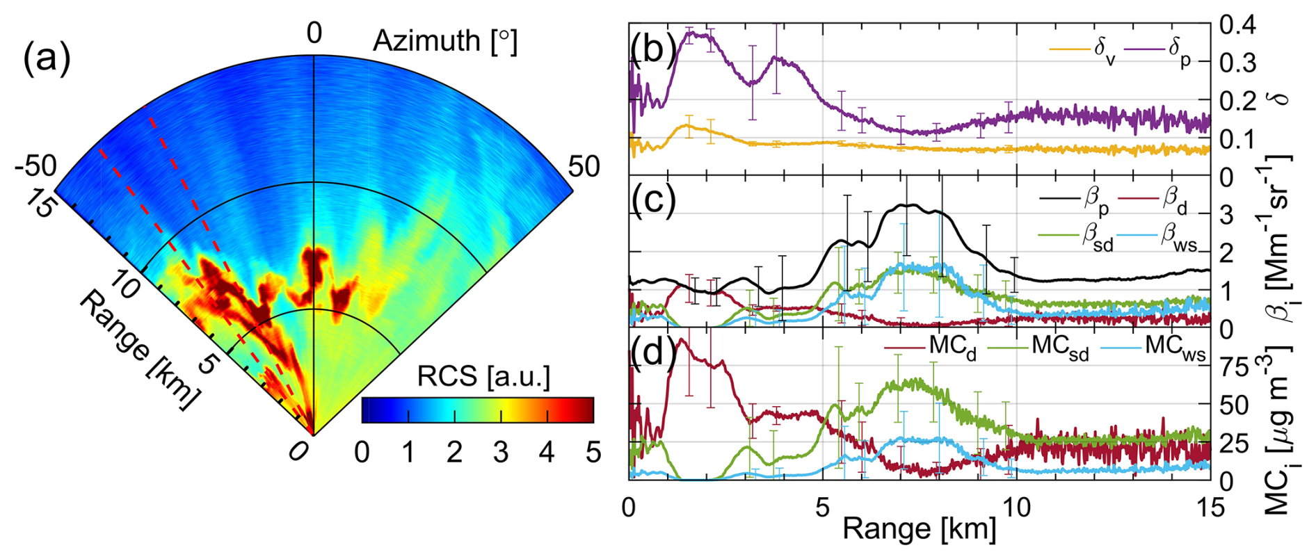
Figure 6 (a) RA series of the ISPL RCSs on 20 September 2022, 07:43–08:28 LT; 20 signals between the two red dashed lines were averaged to retrieve the profiles of (b) the volume linear depolarization (δ_v) and the particle linear depolarization (δ_p) ratios, (c) backscatter coefficient of dust (β_d), salt-dust (β_sd), wet-salt (β_ws) particles, and their sum (β_p), (d) mass concentration (MC_i) for the same particle types as in (c).

3.1 Case study: a mixture of wet-salt, salt-dust, and dust

Figure 6a is an azimuthal scan of the lidar recorded RCS's on 20 September 2022, 07:43–08:28 local time (LT; UTC +03:30). The lidar Range-Angle (RA) series covers up to a distance of ∼15 km and an angular span of 100°. The Met Office reported mean temperature and surface wind speed are 22 °C and 2 m s⁻¹, respectively, with a relative humidity of 27 % and no cloud coverage. It should be mentioned that September is one of the driest months of the year in the Urmia Lake region (Fig. 1). The presence of an aerosol plume in Fig. 6a is evident, mainly indicated by brownish-red and yellow colors. MODIS imagery together with the Hybrid Single-Particle Lagrangian Integrated Trajectory model (HYSPLIT) back-trajectory analysis reject any possibility for trans-regional aerosol plume transport into the area (not shown here).

For the classification analysis of the aerosols included in the plume, the signals between the two red dashed lines in Fig. 6a were averaged and further examined. The obtained results are presented in Fig. 6b–d. Figure 6b displays the volume (v) and particle (p) linear depolarization ratios, and the particle backscatter coefficient (β_p), which is obtained from the Klett-Fernald Algorithm, is depicted in Fig. 6c for the selected region. Two peaks on δ_p (∼0.30–0.35) within the first ∼5 km, followed by a decrease (δ_p∼0.10) between ∼5 and ∼10 km, indicate the possible presence of dust and salt particles, respectively. Feeding the obtained β_p and δ_p into the modified 2-step POLIPHON (Figs. 3 and 4), the backscatter coefficients for dust, salt-dust, and wet-salt can be retrieved (Fig. 6c). Putting the obtained β_d, β_sd, β_ws and their corresponding parameters of the three particle types from Table 1 into Eq. (2), the mass concentrations of particles, MC_d, MC_sd, and MC_ws will be in reach (Fig. 6d). Figure 6c and d show a dust layer that starts at a distance of ∼1 km, extends up to ∼7 km from the station. Meanwhile, the second part of the plume, which started at a range of ∼4.5 km and spread up to ∼10 km, contains both salt-dust and wet-salt particles. Though β_sd and β_ws are almost the same over the second part of the plume (Fig. 6c), their mass concentrations are quite different; MC_sd reaches up to ∼70 µg m⁻³, but the maximum value of MC_ws is ∼30 µg m⁻³. The mass concentration of dust particles is quite high at ∼1.4 km from the station, which MC_d is getting close to 95 µg m⁻³.

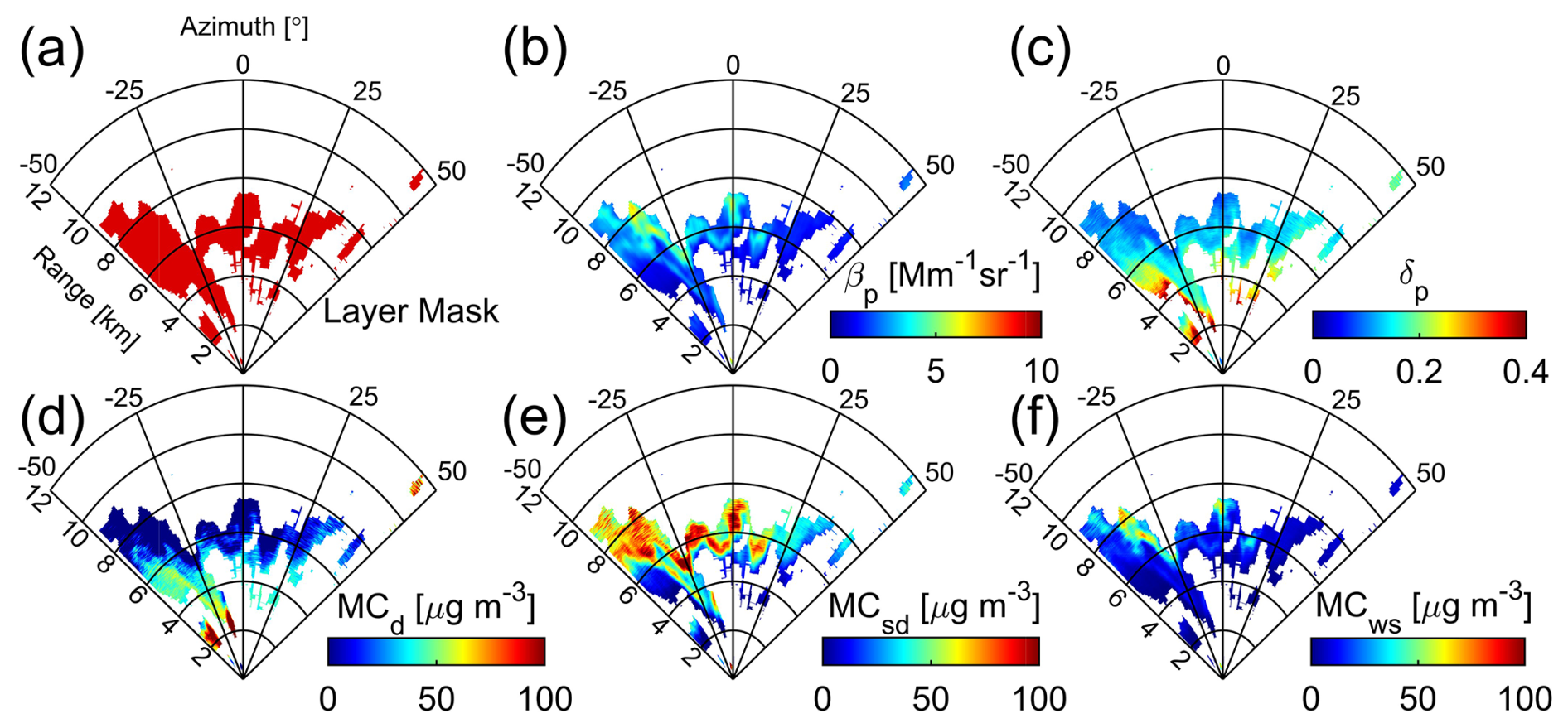
Figure 7 RA series of: (a) the layer mask obtained by applying the MSD algorithm on RCSs recorded by ISPL on 20 September 2022, 07:43–08:28 LT, see Fig. 6a, (b) the particle backscattering coefficient (β_p), (c) particle depolarization ratio (δ_p), and mass concentration profiles of: (d) dust (MC_d), (e) salt-dust (MC_sd), and (f) wet-salt (MC_ws).

The same classification procedure was applied to all scanning directions. The detected aerosol plumes were then selected by using the MSD algorithm and removing the plume-free regions from the RA series of the lidar RCSs. Figure 7a shows the obtained mask when the MSD has been applied to the lidar signals, and Fig. 7b–f are the corresponding spatial profiles of the optical (δ_p and β_p) and physical (MC_d, MC_sd, and MC_ws) parameters of the plume. Figure 7b shows that particles in higher ranges (≳4 km) have a higher backscattering with respect to those close to the lidar station (ranges ≲5 km) that show higher values of δ_p (Fig. 7c). Corresponding mass concentrations of different types of particles in Fig. 7d–f indicate that dust particles are mostly close to the station (Fig. 7d), but salt-dust and wet-salt particles mostly are at ranges beyond ∼4 km. Comparison of Fig. 7e and f indicate that salt-dust particles are dominant in the plume with respect to the wet-salt ones. Taking the MC_is averages over the plume leads to ${\stackrel{\mathrm{‾}}{\mathrm{MC}}}_{\mathrm{d}}=\mathrm{22}\pm \mathrm{27}$, ${\stackrel{\mathrm{‾}}{\mathrm{MC}}}_{\mathrm{sd}}=\mathrm{43}\pm \mathrm{26}$, and ${\stackrel{\mathrm{‾}}{\mathrm{MC}}}_{\mathrm{ws}}=\mathrm{13}\pm \mathrm{11}$ µg m⁻³. Based on the obtained MC_is, the contributions of the three types of aerosols in the plume are 28 %, 55 %, and 17 % for d, sd, and ws particles, respectively. Such average values are calculated for 64 plume-included cases (see Sect. 3.2).

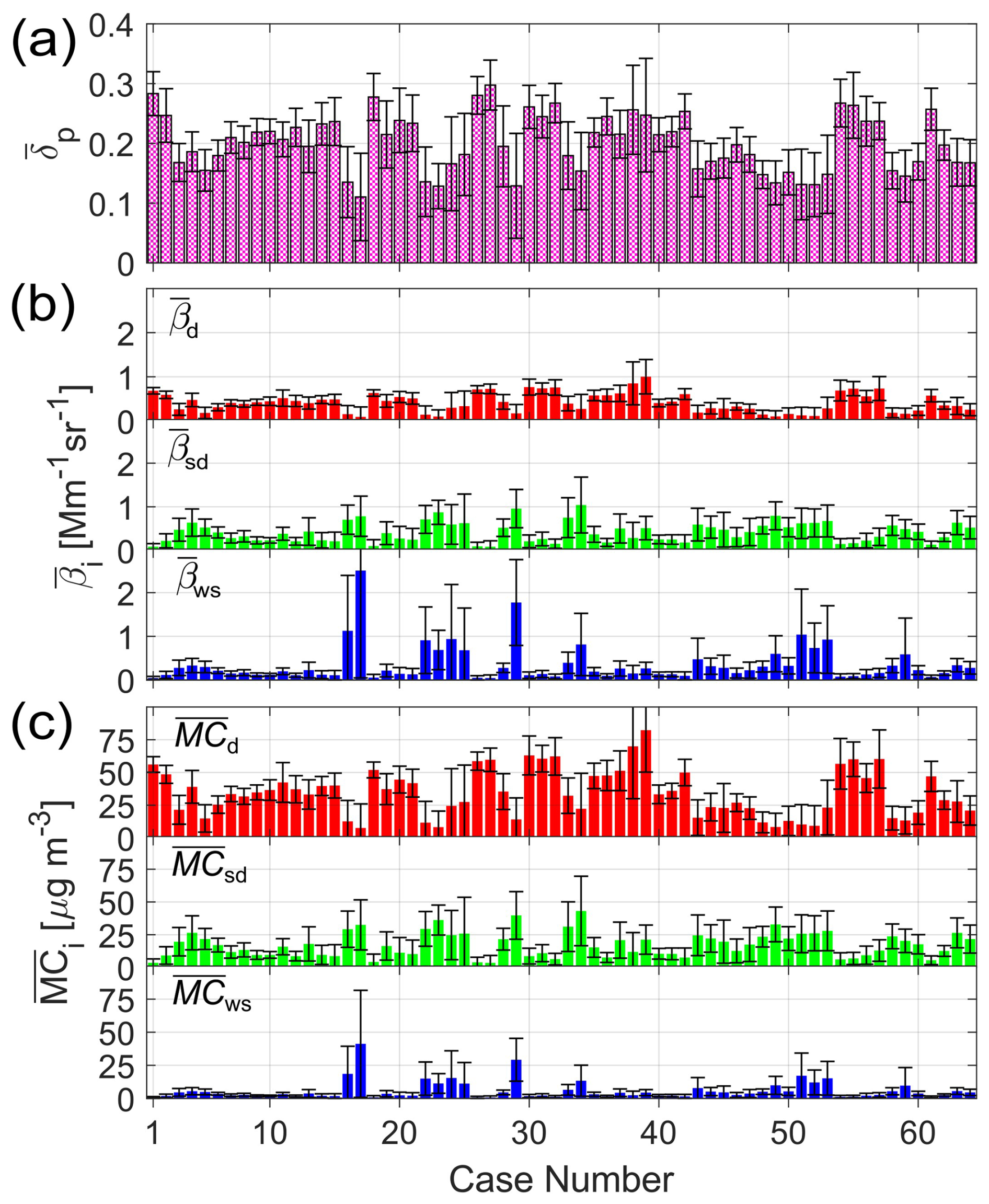
Figure 8 Statistical analyses of 64 cases that contained aerosol plumes, detected by ISPL over the Urmia Lake dried bed atmosphere in September 2022. The plume-averaged values: (a) the particle depolarization ratio (${\stackrel{\mathrm{‾}}{\mathit{\delta }}}_{\mathrm{p}}$), (b) the backscatter coefficient of identified particle types (${\stackrel{\mathrm{‾}}{\mathit{\beta }}}_i$), and (c) their corresponding mass concentrations (${\stackrel{\mathrm{‾}}{\mathrm{MC}}}_i$); i= d, sd, and ws.

3.2 Overall view, 64 cases

During the measurement campaign, 119 scans were performed. Among them, 64 cases contained aerosol plumes. As mentioned in the Sect. 3.1, the physical and optical properties of atmospheric aerosols for each recorded scan that contained a plume are retrieved using the modified 2-step POLIPHON and Eq. (2). Then the MSD algorithm has been applied to all of the 64 cases to isolate the aerosol plume from the background (Mao et al., 2011) and the obtained parameters: δ_p, β_i, and MC_i are averaged over the plume to find ${\stackrel{\mathrm{‾}}{\mathit{\delta }}}_{\mathrm{p}}$, ${\stackrel{\mathrm{‾}}{\mathit{\beta }}}_i$, and ${\stackrel{\mathrm{‾}}{\mathrm{MC}}}_i$. These plume-averaged parameters are depicted in Fig. 8.

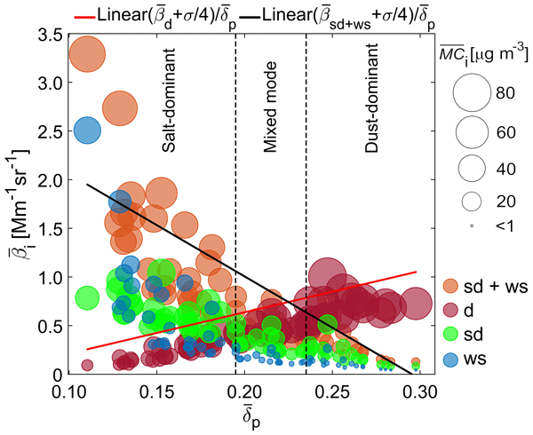
As Fig. 8a shows, ${\stackrel{\mathrm{‾}}{\mathit{\delta }}}_{\mathrm{p}}$ values for all detected aerosol plumes are higher than 0.10. Therefore, all of the plumes should contain dust or salt-dust particles. Some plumes, like those in cases: No. 1, 18, 26, and 27 contained considerable amounts of pure dust particles which ${\stackrel{\mathrm{‾}}{\mathit{\delta }}}_{\mathrm{p}}$ is higher than 0.28. Referring to Fig. 8b and c, ${\stackrel{\mathrm{‾}}{\mathit{\beta }}}_{\mathrm{sd}}$, ${\stackrel{\mathrm{‾}}{\mathit{\beta }}}_{\mathrm{ws}}$, ${\stackrel{\mathrm{‾}}{\mathrm{MC}}}_{\mathrm{sd}}$, and ${\stackrel{\mathrm{‾}}{\mathrm{MC}}}_{\mathrm{ws}}$ are quite small for such cases. On the other hand, for cases like No. 17 and 29, where the plumes contained considerable amounts of salt particles (salt-dust and wet-salt), ${\stackrel{\mathrm{‾}}{\mathit{\delta }}}_{\mathrm{p}}$ decreased to ∼0.12, ${\stackrel{\mathrm{‾}}{\mathit{\beta }}}_{\mathrm{sd}}$, ${\stackrel{\mathrm{‾}}{\mathit{\beta }}}_{\mathrm{ws}}$, ${\stackrel{\mathrm{‾}}{\mathrm{MC}}}_{\mathrm{sd}}$, and ${\stackrel{\mathrm{‾}}{\mathrm{MC}}}_{\mathrm{ws}}$ considerably increased, in contrast, ${\stackrel{\mathrm{‾}}{\mathit{\beta }}}_{\mathrm{d}}$ and ${\stackrel{\mathrm{‾}}{\mathrm{MC}}}_{\mathrm{d}}$ are quite low. Figure 8b and c also show how the salt content of aerosols influences the backscatter coefficient and eventually the albedo of the plume. For example in case 17, ${\stackrel{\mathrm{‾}}{\mathrm{MC}}}_{\mathrm{ws}}\simeq$ 40 µg m⁻³ and ${\stackrel{\mathrm{‾}}{\mathit{\beta }}}_{\mathrm{ws}}\simeq \mathrm{2.5}{\mathrm{Mm}}^{-\mathrm{1}}{\mathrm{sr}}^{-\mathrm{1}}$ but for case 39, when ${\stackrel{\mathrm{‾}}{\mathrm{MC}}}_{\mathrm{d}}\simeq \mathrm{82}$ µg m⁻³ the ${\stackrel{\mathrm{‾}}{\mathit{\beta }}}_{\mathrm{d}}$ is only $\sim \mathrm{1.0}{\mathrm{Mm}}^{-\mathrm{1}}{\mathrm{sr}}^{-\mathrm{1}}$. This is in complete agreement with the lower lidar ratios obtained for salt particles (∼25 sr) compared to dust particles (Table 1).

Table 2 Average values of ${\stackrel{\mathrm{‾}}{\mathit{\beta }}}_i$, ${\stackrel{\mathrm{‾}}{\mathit{\alpha }}}_i$, and ${\stackrel{\mathrm{‾}}{\mathrm{MC}}}_i$ over all 64 cases (the 〈〉 sign) for dust (d), salt-dust (sd), wet-salt (ws), and salt-dust plus wet-salt (sd+ws) particles.

We also calculated the plume averaged extinction coefficients (${\stackrel{\mathrm{‾}}{\mathit{\alpha }}}_i$), using the retrieved ${\stackrel{\mathrm{‾}}{\mathit{\beta }}}_i$ and S_i values in Table 1, then to obtain an overall view on the contribution of different types of particles to the formation of aerosol plumes over the lake, averaged on ${\stackrel{\mathrm{‾}}{\mathit{\beta }}}_i$, ${\stackrel{\mathrm{‾}}{\mathit{\alpha }}}_i$ and ${\stackrel{\mathrm{‾}}{\mathrm{MC}}}_i$ across all 64 cases and for all types of pre-assumed particles, including: dust (d), salt-dust (sd), wet-salt (ws), and a combination of salt-dust and wet-salt (sd+ws). The results are presented in Table 2, where the 〈〉 denotes the average over all 64 cases. Table 2 shows that even though the average values of particle backscatter coefficient for mixtures of wet-salt and salt-dust particles, $\langle {\stackrel{\mathrm{‾}}{\mathit{\beta }}}_{\mathrm{sd}+\mathrm{ws}}\rangle$ is almost twice of $\langle {\stackrel{\mathrm{‾}}{\mathit{\beta }}}_{\mathrm{d}}\rangle$, their averaged mass concentration, $\langle {\stackrel{\mathrm{‾}}{\mathrm{MC}}}_{\mathrm{sd}+\mathrm{ws}}\rangle$, is $\sim \mathrm{2}/\mathrm{3}$ of $\langle {\stackrel{\mathrm{‾}}{\mathrm{MC}}}_{\mathrm{d}}\rangle$. In other words, the salt particles made the main contribution to the formation of aerosol plumes over the lake, but their lower share in the mass concentration is mainly due to the difference in the mass densities and lidar ratios of the salt and dust particles (Table 1). Table 2 also shows that salt particles mostly appear as salt-dust aerosols. To categorize aerosol plumes, we define three new parameters, σ_d and σ_sd+ws as the standard deviations of $\langle {\stackrel{\mathrm{‾}}{\mathit{\beta }}}_{\mathrm{d}}\rangle$ and $\langle {\stackrel{\mathrm{‾}}{\mathit{\beta }}}_{\mathrm{sd}+\mathrm{ws}}\rangle$, respectively, and their sum, $\mathit{\sigma }={\mathit{\sigma }}_{\mathrm{d}}+{\mathit{\sigma }}_{\mathrm{sd}+\mathrm{ws}}$. Then we categorize the plumes into three modes: dust-dominant, salt-dominant, and mixed mode, as Table 3. The number of cases observed in each mode and the probability distribution function (pdf) of each mode are shown in Table 3 columns 3 and 4, respectively. It shows that 47 % of the 64 recorded cases were salt-dominant, while 25 % of them were dust-dominant.

Table 3 Categorization of the recorded aerosol plumes over the Urmia Lake based on the backscatter coefficients of their constituent particles, number, and probability distribution function (pdf) of observed cases in each category.

Solid colored circles in Fig. 9 are the plume-averaged mass concentrations (${\stackrel{\mathrm{‾}}{\mathrm{MC}}}_i$) of different types of aerosols (d-dark red, sd-green, ws-blue, and sd+ws-orange), as functions of the plume-averaged particle linear depolarization ratio (${\stackrel{\mathrm{‾}}{\mathit{\delta }}}_{\mathrm{p}}$) and the backscattering coefficients (${\stackrel{\mathrm{‾}}{\mathit{\beta }}}_i$) for each recorded event. Figure 9 shows clearly that as ${\stackrel{\mathrm{‾}}{\mathrm{MC}}}_{\mathrm{d}}$ increases, ${\stackrel{\mathrm{‾}}{\mathit{\delta }}}_{\mathrm{p}}$ increases too, but ${\stackrel{\mathrm{‾}}{\mathit{\delta }}}_{\mathrm{p}}$ has a reverse relation with variations of salt particle mass concentrations (sd, ws, and sd+ws). Interestingly, salt particles have a significantly greater influence on particle backscatter coefficients. For instance, Fig. 9 shows the backscattering coefficient for ${\stackrel{\mathrm{‾}}{\mathrm{MC}}}_{\mathrm{ws}}\simeq \mathrm{40}$ µg m⁻³ is about 2.5 ${\mathrm{Mm}}^{-\mathrm{1}}{\mathrm{sr}}^{-\mathrm{1}}$ while similar mass concentrations of dust particles have ${\stackrel{\mathrm{‾}}{\mathit{\beta }}}_{\mathrm{d}}<\mathrm{0.5}$ ${\mathrm{Mm}}^{-\mathrm{1}}{\mathrm{sr}}^{-\mathrm{1}}$.

The black and red solid lines are fits to variations of ${\stackrel{\mathrm{‾}}{\mathit{\beta }}}_{\mathrm{sd}+\mathrm{ws}}+\frac{\mathit{\sigma }}{\mathrm{4}}$ and ${\stackrel{\mathrm{‾}}{\mathit{\beta }}}_{\mathrm{d}}+\frac{\mathit{\sigma }}{\mathrm{4}}$ vs ${\stackrel{\mathrm{‾}}{\mathit{\delta }}}_{\mathrm{p}}$, respectively. As Table 3 indicates, these two lines are used to categorize the aerosol plumes. This categorization somehow determines borders on ${\stackrel{\mathrm{‾}}{\mathit{\delta }}}_{\mathrm{p}}$ for each category of the aerosol plumes. Two black vertical dashed lines in Fig. 9 show these borders. Using these borders, it can be found that the average values of ${\stackrel{\mathrm{‾}}{\mathit{\delta }}}_{\mathrm{p}}$ for the salt-dominant, dust-dominant, and mixed mode aerosol plumes are 0.16±0.02, 0.26±0.02, and 0.22±0.01, respectively.

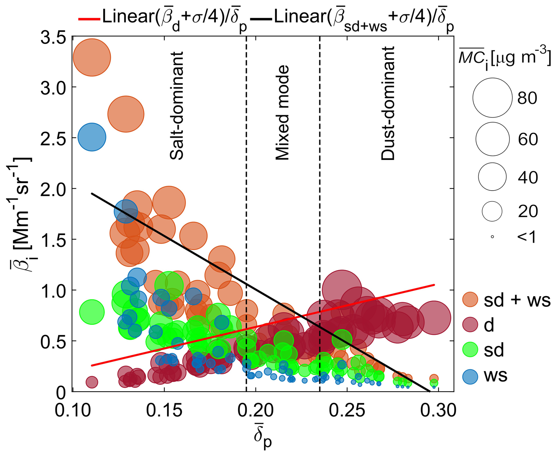
Figure 9 The scatterplot of plume-averaged backscattering (${\stackrel{\mathrm{‾}}{\mathit{\beta }}}_i$) versus plume-averaged depolarization ratio (${\stackrel{\mathrm{‾}}{\mathit{\delta }}}_{\mathrm{p}}$) for different particles. Color of the circles indicates particle type: dark red-d, green-sd, blue-ws, and orange-sd+ws. The circle size corresponds to ${\stackrel{\mathrm{‾}}{\mathrm{MC}}}_i$. The Red and black solid lines are fits on $({\stackrel{\mathrm{‾}}{\mathit{\beta }}}_{\mathrm{d}}+\frac{\mathit{\sigma }}{\mathrm{4}})/{\stackrel{\mathrm{‾}}{\mathit{\delta }}}_{\mathrm{p}}$ and $({\stackrel{\mathrm{‾}}{\mathit{\beta }}}_{\mathrm{sd}+\mathrm{ws}}+\frac{\mathit{\sigma }}{\mathrm{4}})/{\stackrel{\mathrm{‾}}{\mathit{\delta }}}_{\mathrm{p}}$. Based on column 2 of Table 3, two black dashed lines separate the regions where dust or salt particles are dominant or a mixture of them is in the detected plume.

4 Summary and conclusions

This study provides new observational evidence on the contributions of salt-dust plumes originating from the desiccated bed of Urmia Lake to the regional aerosol load. For the first time, the near-surface atmosphere over Urmia Lake was monitored using a scanning polarization lidar system. Nighttime lidar measurements at a wavelength of 532 nm were conducted in September 2022 with the lidar operating in azimuthal scan mode. These observations captured the temporal and spatial evolution of aerosol plumes rising near the surface of Urmia Lake. Observations confirmed the presence of both dust and saline particles in the atmosphere during the measurement period. The modified 2-step POLIPHON algorithm, Figs. 3 and 4, was applied to the recorded lidar signals (for example, Fig. 6), and subsequently to the complete azimuthal scans to find the backscattering ratios and mass concentrations of dust, salt-dust, and wet-salt particles. Then, to distinguish the aerosol plume from the plume-free atmosphere, we used the MSD algorithm. The particle depolarization ratios, backscattering coefficients, and mass concentrations of different particles, which are retrieved from the lidar signals (e.g., Fig. 6), are averaged over each specified aerosol plume to find the contribution of various particle types to the formation of the plume (e.g., Figs. 8 and 9). The analyses revealed the presence of saline particles such as salt-dust and wet-salt aerosols, characterized by lower depolarization ratios but exhibiting higher backscatter coefficients with respect to the pure dust particles (see Figs. 8 and 9). By putting conditions on plume-averaged backscatter coefficients of different types of particles, we have been able to divide the plumes into three categories: dust-dominant, salt-dominant, and mixed mode (Table 3). Statistical analysis of 64 plumes (Table 3) revealed that 47 % of all recorded cases were salt-dominant, 25 % dust-dominant, and the remaining 28 % of the cases were in mixed mode. When these conditions are applied to variations of plume-averaged mass concentrations and backscattering coefficients of different aerosol types with respect to their plume-averaged particle depolarization ratio (Fig. 9), specific ranges are determined for ${\stackrel{\mathrm{‾}}{\mathit{\delta }}}_{\mathrm{p}}$ of each plume type. In results, the average value of ${\stackrel{\mathrm{‾}}{\mathit{\delta }}}_{\mathrm{p}}$ for dust-dominant, salt-dominant, and mixed mode obtained as 0.26±0.02, 0.16±0.02, and 0.22±0.01 respectively. These results highlight that even relatively low mass concentrations of salty particles can substantially increase the atmospheric backscattering coefficient over the dried bed of Urmia Lake. This finding carries important implications for atmospheric radiative transfer studies (Murphy et al., 1998; Murayama et al., 1999; Carrico et al., 2003; Ayash et al., 2008; Zakey et al., 2008; Lundgren et al., 2013). In short, we not only characterized the contributions of different particle types to the observed aerosol plumes over Urmia Lake, but we also categorized the plumes and showed how salt particles influence plume albedo. We hope to implement this technique in our future works to track the advection of salt particles from the lake into neighboring regions, to find how the desiccated lake may impact the cities and other regions in its catchment area. To do this, other measurement campaigns should be run on other locations in the Urmia Lake catchment area, especially in the regions between the lake and the city of Tabriz, which is the largest city in Northwest Iran, hosting about 1.7 million inhabitants, and a considerable number of industries are active in its suburbs. Such campaigns should be carried out on the east side of the lake.