the Creative Commons Attribution 4.0 License.
the Creative Commons Attribution 4.0 License.
 | 21 Jan 2026
Have you ever seen the rain? Observing a record convective rainfall with national and local monitoring networks and opportunistic sensors
Louise Petersson Wårdh
Hasan Hosseini
Remco van de Beek
Jafet C. M. Andersson
Hossein Hashemi
Jonas Olsson
Short-duration extreme rainfall can cause severe impacts in built environments and flood mitigation measures require high-resolution rainfall data to be effective. It is a particular challenge to observe convective storms, which are expected to intensify with climate change. However, rainfall monitoring networks operated by national meteorological and hydrological services generally have limited ability to observe rainfall at sub-hourly and sub-kilometer scales. This paper investigates the capability of second- and third-party rainfall sensors to observe a highly localized convective storm that hit southwestern Sweden in August 2022. Specifically, we compared the observations from professional weather stations, C-band radar, X-band radar, Commercial Microwave Links and Personal Weather Stations to get a full impression of the sensors' strengths and weaknesses in the context of convective storms. The results suggest that second- and third-party networks can contribute important information on short-duration extreme rainfall to national weather services. The second-party network assisted in quantifying the magnitude and spatial variability of the event with high accuracy. The third-party network could contribute to the understanding of the duration and spatial distribution of the storm, but it underestimated the magnitude compared with the reference sensors.
- Article
(4128 KB) - Full-text XML
- BibTeX
- EndNote


The global trend of urbanization is increasingly exposing people and assets to flood risks, which particularly affects the urban poor (Winsemius et al., 2018; Petersson et al., 2020; UN-Habitat, 2024). Flood mitigation and disaster preparedness measures require rainfall measurements on sub-hourly and sub-kilometer scales to be effective from the planning phase to post-event analysis (Guo, 2006; Marchi et al., 2009; Mailhot and Duchesne, 2010; Fuentes-Andino et al., 2017; Pulkkinen et al., 2019; Imhoff et al., 2020). However, traditional monitoring techniques generally have limited ability to accurately observe rainfall at this spatiotemporal resolution. The most impactful rainfall events in urban areas are typically convective storms, which can cause heavy rain over small areas and short durations with severe damage as a consequence (Kaiser et al., 2021; Mobini et al., 2021).
In Sweden, the Swedish Meteorological and Hydrological Institute (SMHI) operates around 600 rain gauges across a landmass of 410 000 km2. Of these, around 130 are automatic stations recording accumulated rainfall depth every 15 min, and the remaining are manual stations reporting daily amounts. The station network is complemented with 12 C-band Weather Radars (CWR) across the country with outputs every 5 min at 2 km spatial resolution. While CWR generally is capable of producing a good spatial representation of precipitation, it has limitations caused by beam overshooting, beam blockage and clutter (van de Beek et al., 2016; Einfalt et al., 2004). For highly localized convective events, the spatiotemporal resolution of Sweden's official gauge network and radar composite is too low to capture essential rainfall dynamics, such as spatial variability and peak intensity.
One option for national meteorological and hydrological services (NMHS) to access high-resolution rainfall measurements is to reach agreements with other professional entities like municipal water utilities and universities that maintain their own monitoring networks, so-called “second-party data” (Garcia-Marti et al., 2023). While these data might be trustworthy for operational use, their sampling resolution may, just like official data, be insufficient on the “unresolved spatial scale” in which convective storms occur (Lussana et al., 2023). In light of this, SMHI has recently gained interest in additional external observations not operated by any official agency, sometimes referred to as “third-party data”. The new technologies are often enabled by digitalization and user-generated content on the Internet, which lowers the barriers and costs associated with data acquisition. While these data can provide higher resolution observations in space and time, they are often subject to uncertainties and bias due to the lack of installation guidelines, maintenance protocols and mechanisms to reinforce such standards. These promises and concerns have sparked research efforts on applications and quality control of third-party data at SMHI and many other European NMHS (Hahn et al., 2022; Garcia-Marti et al., 2023; Olsson et al., 2025).
This paper investigates the capability of second- and third-party rainfall sensors to observe a highly localized convective storm that occurred on 18 August 2022 in Båstad, Sweden. The second-party data comes from sensors managed by local authorities in Skåne County and consists of a traditional rain gauge and an X-band Weather Radar (XWR). As for third-party data, we study rainfall observations from a Commercial Microwave Link (CML) and a set of Personal Weather Stations (PWS). CML and PWS are sometimes referred to as “opportunistic sensors” (Fencl et al., 2024). Here, we will use the term “third-party data” for consistency. First, the long-term (2021–2022) performance of the second-party rain gauge is evaluated against the national weather stations to qualify as a trusted reference sensor for the study. Then, an event analysis is performed by calculating evaluation metrics for each sensor compared with the reference. Data from the radars and third-party sensors require pre-processing and quality control to facilitate the analysis.
XWRs are lower-cost compared with conventional C-band and S-band weather radars and provide higher resolution imagery. They are, on the other hand, more affected by attenuation, especially in widespread heavy rainfalls due to the accumulated attenuation throughout the signal path (Lengfeld et al., 2016; Bobotová et al., 2022). XWRs also have a shorter observation range than conventional radars, typically 30–60 km (Thorndahl et al., 2017).
CMLs are radio links between base stations that connect the backbone of telecom networks to local subnetworks (Chwala and Kunstmann, 2019). CMLs operate at frequencies where the propagation of radio waves through the atmosphere is attenuated by rainfall. The transmitted signal level (TSL) and received signal level (RSL) are collected by telecom companies for network monitoring and maintenance purposes, so what is being considered as “noise” in telecommunication can be used as a signal to estimate rainfall intensities for hydrometeorological applications (Leijnse et al., 2007b). In this paper we study the spatial variability of rainfall along a CML link by sampling XWR bins every 250 m along the CML reach, resulting in 20 XWR time series that are compared with the CML rainfall estimates. This approach enables us to perform detailed investigations about bias in CML observations due to the variability of rainfall intensity along a CML path.
PWS are weather stations installed by people on their private property. Here, we consider PWS that can be connected to online platforms to share observations openly in real time. Recent years have seen a remarkable increase in PWS connected to the internet, presumably due to the adoption of smart home technologies (Sovacool and Furszyfer Del Rio, 2020). Contrary to CML, PWS are designed to measure rainfall directly, but it can be assumed that PWS data are subject to errors and bias linked to hardware, installation site and maintenance (Boonstra, 2024). Various quality control protocols explicitly designed for PWS have been presented in the literature (de Vos et al., 2019; Bárdossy et al., 2021; Lewis et al., 2021). However, it has not been investigated how the algorithms perform when applied to localized extreme rainfall. In this paper, we apply an adjusted version of the PWS quality control protocol suggested by de Vos et al. (2019) and compare the results with traditional evaluation metrics.
This paper addresses multiple gaps in high-resolution monitoring of convective rainfall by bench-marking second- and third-party sensors with an official monitoring network, and by investigating the performance of a PWS quality control protocol in this context. The study is guided by an ambition to contribute to answering the following general research questions:
-
To what extent are second- and third-party sensors capable of observing convective rainfall?
-
What are the advantages and limitations of observing convective rainfall with second- and third-party sensors, compared with a national monitoring network?
This paper is organized as follows. After this introductory section, Sect. 2 presents the storm event and area of interest that was selected for the case study. Section 3 describes the sensors and data applied in the analysis. Section 4 presents evaluation metrics and methods applied for the long-term and event analysis. Section 5 outlines the results of the long-term and event analysis. Section 6 discusses the results, while Sect. 7 summarizes the main findings of the study.
A convective rainfall event that hit the Bjäre Peninsula in Skåne County, Sweden, in the late afternoon of 18 August 2022, was selected for the study. SMHI's forecast had indicated a small likelihood of rainfall intensities above 35 mm/3 h, which is the institute's threshold for rainfall weather warnings. However, it was expected to hit further to the north, so no weather warning was issued in the area at the time of the event. According to media reports, the rain was mixed with hailstones of about 2 cm in diameter and caused flooding of around 60 buildings (Gravlund, 2025; Bengtsson, 2023). A local water utility company (NSVA) operates a tipping bucket rain gauge (hereafter “municipal gauge”) in the city of Båstad, which peaked at 216 mm h−1 and recorded 75.4 mm in 64 min. This corresponds to a return period of about 700 years, based on rainfall statistics developed for southwestern Sweden (Olsson et al., 2019). The maximum depth recorded in 45 min was 71.2 mm, which breaks Sweden's official record of 61.1 mm in 45 min at the Daglösen station in Värmland County on 5 July 2000. The predominant wind direction in the area is from the southwest to the northeast, and the selected event was preceded by two dry days. The analysis focused on the urban area of Båstad, a town with around 16 000 inhabitants located on the southern coast of the Laholm Bay, covering approximately 9.4 km2. Figure 1 shows the locations of all sensors included in the study.
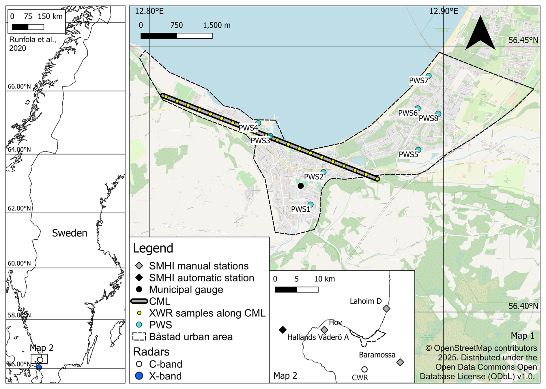
Figure 1Area of interest and locations of sensors (map data from OpenStreetMap, https://www.openstreetmap.org/copyright, last access: 2 November 2025).
Three levels of data were considered in the study – Sweden's national meteorological monitoring network, a municipal gauge and XWR operated by local and regional agencies (second-party network) and CML and PWS (third-party network). More details on the data sets are provided below.
3.1 National monitoring network
The national weather monitoring network operated by SMHI consists of a combination of manual and automatic weather stations and CWR. The Hov, Laholm D and Baramossa weather stations, located 9–10 km away from Båstad (Fig. 1), report daily accumulated rainfall at 06:00 UTC+2, manually observed by certified observers. The automatic rain gauge station of weighing type on the island Hallands Väderö, situated 15 km west of Båstad, reports 15 min accumulations. As these data have passed quality assurance protocols at SMHI, we consider them the most trustworthy source to use for benchmarking in the study. Precipitation data from the stations for the year 2022 were downloaded from SMHI's open data archive (SMHI, 2025b).
In addition, we studied a gauge-adjusted Plan Position Indicator (PPI) horizontal reflectivity composite based on the lowest elevation scan (0.5°) from all radars operated by SMHI. The composite is used operationally for weather forecasting at the institute. The composite is available in 5 min resolution at a spatial resolution of 2×2 km and distributed as radar reflectivity data in SMHI's open radar archive (SMHI, 2025c).The gauge-adjustment technique is based on the gauge-to-radar ratio and is targeted towards real-time applications (refer to Michelson and Koistinen, 2000, for details). Radar data compositing at SMHI is performed using the BALTRAD software (Michelson et al., 2018). While the radars can operate in dual-polarization mode, this product is based on the horizontal polarization. The closest radar (radar location Ängelholm) is situated 6 km south of Båstad (Fig. 1, map 2). Since this radar was operational during the selected event and the compositing method is based on the closest radar, the studied composite is based on data from only this radar during the period of interest.
Radar reflectivity Z [mm6 m−3] can be expressed as integrals over the Drop Size Distribution (DSD) in the pulse volume, here N(D) [mm m−3].
where D [mm] is the spherical drop diameter. It is generally expressed logarithmically as dBZ:
The CWR composite retrieved from SMHI's radar archive is distributed as pseudo-dBZ E (integer 0–255) to enable a smaller storage size, following European standards (Michelson et al., 2014). To convert these integers back to dBZ, gain G and offset were applied:
where G=0.4 and offset = −30 (Michelson et al., 2014). The rain rate PCWR (mm h−1) can be found from the reflectivity following an inverted power law relationship:
We applied the parameters suggested by Marshall and Palmer (1948), a=200 and b=1.6. The actual values of a and b can vary greatly depending on the actual DSD, which may be different within and from event to event (Battan, 1973). CWR time series at a 5 min resolution were sampled at the locations of the municipal rain gauge and the eight PWS.
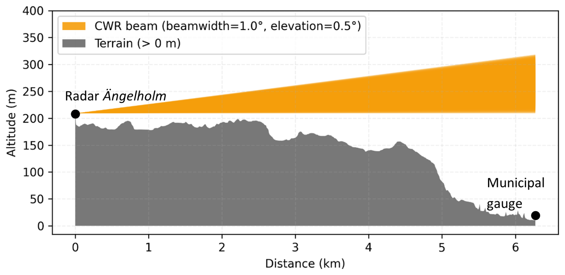
Figure 2Elevation profile and beam profile between the CWR radar location and the municipal gauge.
Figure 2 shows the elevation profile and radar beam profile between the CWR location and the location of the municipal gauge in Båstad. The low elevation angle and short distance to the area of interest indicate that the observations are made at approximately 200–300 m a.s.l. (above sea level), eliminating the risk of beam overshooting, as convective precipitation in the summer months typically originates from much higher altitudes. Overshooting is a common error in radar data that appears when the radar beam shoots above the precipitation cloud (Battan, 1973; Seo et al., 2000). However, the Ängelholm radar is affected by partial beam blockage in a circular sector of around 60° to the north of the radar location, which covers the area of interest (Appendix A1., Fig. A1). This is caused by vegetation within 1 km north of the radar location (Appendix A1, Fig. A2). Evaluations at SMHI have shown that the Ängelholm radar underestimated the accumulated rainfall depth of the years 2022–2023 by around 80 % in the affected area, compared with SMHI's weather stations.
3.2 Second-party monitoring network
We consider two second-party sensors operated by local and regional authorities: a municipal gauge in Båstad managed by the local water utility company NSVA, and a compact FURUNO dual-polarization XWR operated by NSVA on behalf of Lund University. The municipal gauge is a Casella tipping bucket, which records a tip each time the bucket volume (0.2 mm) is filled on a 1 s resolution. Time series with 1 min resolution from the municipal rain gauge for the years 2021–2022 were received upon request from NSVA.
About 80 % of Skåne County is covered by observations from two XWRs located in Dalby and Helsingborg (Hosseini et al., 2023). In this study, we used data from the XWR in Helsingborg, 40 km south of Båstad (Fig. 1). The spatial resolution of the data is 0.5° of azimuth and 75 m of slant range. XWR data for the day of the event was acquired from VeVa (Weather Radar in the Water Sector) (Foreningen VeVa, 2025), a collaboration between water utility companies in south Sweden and Denmark that distributes XWR data to its partners according to the EUMETNET Opera Data Information Model (Michelson et al., 2014).
The manufacturer's built-in precalculated rainfall rate PXWR (mm h−1) from the lowest scan (elevation angle of 1°) on 1 min resolution was used for the study. The underlying equations for calculating the rainfall rate are generally similar to CWR as described in Sect. 3.1. However, a main difference is that the XWR data integrates dual-polarization variables as a method for attenuation correction, as described in detail in Hosseini et al. (2020). This method estimates attenuation as an approximately linear function of the specific differential phase shift, which depends on phase rather than signal intensity and is therefore less sensitive to attenuation (Kumjian, 2013). The method has been shown to be useful for summer precipitation estimations in Sweden (Hosseini et al., 2023).
Figure 3 shows that the XWR's beamwidth has a much larger sampling volume and steeper elevation angle than CWR (Fig. 2) at the area of interest, which suggests a small risk of signal contamination due to beam blockage. As the profile extends 250–1750 m a.s.l. over Båstad, this, just like for CWR, suggests a small risk of beam overshooting.
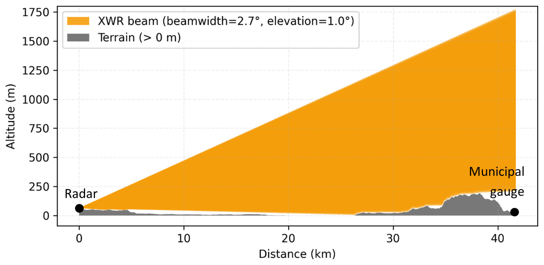
Figure 3Elevation profile and beamwidth between the XWR radar location and the municipal gauge.
3.3 Third-party monitoring network
Two types of third-party sensors were included in the study – CML and PWS. The location of the only CML in the area of interest is shown in Fig. 1. This link is approximately 4.8 km long and has a frequency of 23.1 GHz. CML data were received as TSL and RSL at 10 s resolution upon request from the telecom companies Ericsson AB and Tre. The data covered all base stations on the Bjäre Peninsula for the days 18–19 August 2022. Each antenna works as both a transmitting and receiving terminal, meaning that each link has bidirectional transmission and provides at least two radio signals. Here, we use the term “sub-link” to refer to a single radio signal.
Received TSL and RSL were converted into rainfall rate using the MEMO (Microwave-based Environmental Monitoring) method developed by SMHI; MEMO, 2025). This method follows the general steps applied by most CML algorithms as described in Appendix A2. However, the process does not explicitly correct for wet antenna attenuation, but instead applies a bias correction factor CFA based on link length to the derived rain rate Praw (mm h−1) that compensates for the wet antenna effect:
Here, Praw is the uncorrected rainfall intensity and Anl is the net attenuation. More details on CML processing are found in Appendix A2.
The selected PWS type in this study, NetAtmo, is an unheated plastic tipping bucket rain gauge that reports the number of tips through a wireless connection to the accompanying indoor module (de Vos et al., 2019). The indoor module broadcasts the observations to Netatmo's online platform at approximately 5 min intervals. The default tipping bucket volume is 0.101 mm, or another volume specified by the station owner using the product's calibration feature. PWS time series for the study were received from NetAtmo. PWS without a rainfall sensor, and PWS that were offline during the storm event, were excluded from the analysis. This resulted in a total of eight PWS located within the Båstad urban area (Fig. 1). The PWS data were quality controlled as described in Sect. 4.4.
The analyses covered two stages – a long-term analysis and an event analysis. This section first presents the evaluation metrics applied to assess the performance of the sensors in the study, followed by descriptions of the methods applied in the long-term analysis and event analysis. Then, the quality control of PWS data is described, as well as time lags applied to the radar data.
4.1 Evaluation metrics
Three evaluation metrics were used to assess the performance of each sensor: Spearman's rank correlation (rs), Root Mean Squared Error (RMSE), and Percent Bias (PBIAS). The metrics were calculated on different temporal resolutions in different analyses, see Sect. 4.2 and 4.3. For each analysis, the metrics were calculated for the duration of the event as recorded by the respective reference sensor, see Sect. 4.3.
The Spearman correlation is a non-parametric test that measures the strength of a monotonic relationship between two variables:
where di is the difference between ranks for each pair of values and n is the number of observations. The closer to −1 or 1, the better the negative or positive monotonic relationship. As the Spearman correlation does not address the magnitude of error, it can be complemented with RMSE (Hyndman and Koehler, 2006):
where Oi is the reference rainfall and Ti is the evaluated data. Lower RMSE indicates a better model performance. Finally, PBIAS quantifies the average bias, where a positive or negative value suggests an underestimation or overestimation of rainfall depth, respectively (Gupta et al., 1999):
4.2 Long-term analysis
As the magnitude of the selected event was not captured by the national network (see Sect. 5) it was necessary to establish another reliable reference for the event analysis. Consequently, the long-term (2021–2022) performance of the municipal gauge was evaluated against the national weather stations using the metrics presented in Sect. 4.1 at daily resolution. The gauge was cross-referenced with the manual stations Hov, Laholm D and Baramossa operated by SMHI, all situated 9.3–9.7 km away (Fig. 1). The station Hallands Väderö A was excluded from the comparison as it is located on an island 15 km west of Båstad. The tips recorded by the municipal gauge were resampled to daily accumulations between 06:00–05:59 UTC+2, as this is the sampling frequency of the reference (manual) stations.
4.3 Event analysis
The temporal range of the studied event differed between each sensor, as the start and end of the rainfall occurred at different times in the observed time series. The reference used for each comparison is outlined below. The event start was defined as the first timestep when it had been raining more than 0.1 mm h−1 for at least 5 min at the reference sensor, and the event stop was when it had been raining less than 0.1 mm h−1 for at least 5 min (Sect. 5.2.1). The return period of the event was calculated based on SMHI's climate statistics for southwestern Sweden (Olsson et al., 2019). The calculation of evaluation metrics, return periods, and accumulated depths were carried out for the duration of the event as recorded by the reference sensor.
Based on performance, it was decided to exclude CWR as a reference (Sect. 5.2.2). The CWR composite was sampled at the location of the municipal gauge, and the metrics were calculated at 5 min resolution (the resolution of the CWR data) with the municipal gauge as the reference. The accumulated rainfall DCWR (mm) was then calculated at the location of the municipal gauge and for the whole CWR composite in the area of interest.
The XWR data were available in polar bins, that is, range gates at a given elevation and azimuthal angle, in contrast to the regular Cartesian grids for the utilized CWR data. Thus, time series were extracted from the XWR polar bin closest to the projected locations of interest, accounting for elevation, range difference, and azimuth difference. The sampled locations included the municipal gauge, the eight PWS, and 20 points along the CML path, as described below. The elevation metrics were calculated on the XWR time series sampled at the municipal gauge on a 5 min resolution with the municipal gauge as reference. After concluding that XWR recorded similar rainfall depth as the municipal rain gauge during the event, XWR was used as a reference for CML and PWS to better account for the spatial variability of the rainfall. For visualization purposes, the volumetric XWR data was gridded into a Cartesian grid of 250 m resolution using linear interpolation with Delaunay triangulation. The accumulated rainfall DXWR (mm) was calculated for the whole area of interest based on the gridded data.
A few missing values were found in the XWR time series, which occurred during the most intense part of the storm. Investigations showed that these bins likely observed rainfall intensities above 255 mm h−1, which is the upper limit for storing integers in 8-bit format and which was used by VeVa when calculating the rain rate. The missing values were filled with temporal linear interpolation.
The CML included in this study consists of two sub-links. These recorded similar values, with a difference in total rainfall depth of around 5 % for the whole event. Thus, the mean rain rate PCML and mean depth DCML per timestep of the two sub-links were used in the analysis. The XWR polar bins data were sampled every 250 m (20 points, Fig. 1) along the reach of the CML to investigate the variability of rainfall intensity along the link, resulting in 20 XWR time series on 1 min resolution. Evaluation metrics were calculated on 1 min resolution with the mean of 20 XWR samples, PXWR, as reference.
To investigate how CML estimates of extreme rainfall are impacted by spatial variability along the link, the 10th and 90th percentiles were calculated to explore the range of PXWR and DXWR along the CML path. The behavior of the XWR data along the CML during the intense part of the storm was inspected visually. Hypothesizing that the difference in XWR and CML observations is related to the XWR variability along the link, an ordinary least squares analysis was performed on the difference PXWR and PCML, with the XWR standard deviation as the independent variable.
For each PWS, the evaluation metrics were calculated compared with the XWR time series sampled at the PWS location on 5 min resolution. The PWS timeseries were processed with a quality control package as described below.
4.4 PWS quality control
Research has shown that the quality of rainfall data from PWS can be improved significantly by applying quality control and bias correction. The algorithms suggested in literature, e.g, Mandement and Caumont (2020), Lewis et al. (2021), Bárdossy et al. (2021), typically utilize the high observation density of PWS by comparing rainfall time series with the performance of neighboring stations, referred to as “buddy checks” by Båserud et al. (2020). de Vos et al. (2019) developed a quality control protocol for PWS rainfall data in the R programming language, PWSQC. The method does not rely on a primary monitoring network, but flags suspicious measurements based on the observations from nearby stations. The method has been applied in gauge-adjustment of radar by Nielsen et al. (2024) and Overeem et al. (2024) and has recently been converted to a Python package, pypwsqc, that was applied for the study (Graf et al., 2025).
Event time series from the eight PWS were processed with pypwsqc. The algorithm applies three filters utilizing neighbor checks – the Faulty Zeroes filter, High Influx filter, and Station Outlier filter – to assess the quality of each time step in rainfall time series by comparing with the records of neighboring PWS within a user-defined radius (refer to de Vos et al., 2019, for details). The Faulty Zeroes filter flags timesteps when the evaluated station records zero rainfall for at least nint time intervals, while the median of the surrounding rainfall observations is larger than zero. The High Influx filter identifies unrealistically high rainfall amounts based on a comparison with the median rainfall of the neighboring stations. The Station Outlier filter flags a station as an “outlier” if the Pearson correlation with the median rainfall of neighbors in a selected evaluation period falls below a set threshold.
To improve the performance of the neighboring checks, data from all PWS within a 10 km radius around Båstad were considered, which resulted in a total of 58 stations. However, only the results of the 8 PWS within the area of interest were evaluated during the event. To get a better understanding of the long-term performance of each PWS, the quality control was also applied for the full year of 2022. The parameters were set to the same values as in the original publication (de Vos et al., 2019), except mmatch and mint. These parameters control how many wet time steps at the evaluated PWS that must be overlapping with wet time steps at the neighboring stations within a defined evaluation period to reliably apply the Station Outlier filter. The numbers proposed by de Vos et al. (2019) were found to be too strict for the PWS dataset in this study, as the Station Outlier filter could not be applied for very long periods, including during the studied storm event. Instead, mmatch and mint were set to 100 and 8064, respectively, to require less wet time steps during a longer evaluation period.
4.5 Time lags
The event analysis revealed low correlations (rs) between the radars (CWR and XWR) and the reference (municipal gauge), see Sect. 5.2.2 and 5.2.3. As convective rainfall is highly variable in space and time, the observations per time step can be very different at nearby locations, which can lead to low correlations even between high-quality observations. Therefore, time lags were applied to the radar time series to see if this could increase the correlation. The radar time series sampled at the municipal gauge were shifted from −10 to +10 timesteps on a 5 min resolution. For each lag, the correlation rs with the municipal gauge was calculated over the event duration as defined by the reference. The highest correlation value was then reported.
5.1 Long-term analysis
Figure 4 shows daily accumulations from the Hov, Laholm D and Baramossa weather stations and the municipal gauge for the years 2021 and 2022. The plot shows that the municipal gauge recorded significantly less rainfall than Baramossa but followed Hov and Laholm D reasonably well. These findings align with rainfall observations of the region in the period 1991–2020 (SMHI, 2025d). The inland regions of southwestern Sweden, including the northern parts of Skåne County where Baramossa is located, overall receives more precipitation than the coastal area, where the Båstad, Hov and Laholm stations are located.
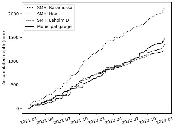
Figure 4Accumulated depth 2021–2022 for municipal gauge and SMHI rain gauges located 9.3–9.7 km away.
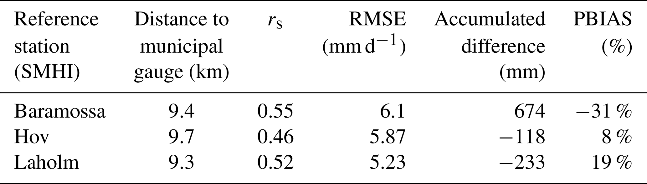
Table 1 shows the evaluation metrics of the municipal gauge, benchmarked with the three reference stations. The PBIAS over 2 years was only −8 % compared with Hov weather station, which is considered low as the stations are situated 9.7 km apart. Based on these results, the municipal gauge was accepted as a trusted reference for the event analysis.
Table 1Cross-validation of the municipal gauge with three reference stations, 2021–2022.
5.2 Event analysis
5.2.1 Event duration
Table 2 summarizes the event duration observed by each sensor. National weather stations were excluded from the analysis, either because they record daily precipitation, or because they recorded very small total depth (Sect. 5.2.2). The municipal gauge recorded rainfall for 64 min, which is among the shortest durations with only PWS 4 observing rain for a shorter period (50 min). Notably, XWR recorded rain for 109 min at the location of the municipal gauge. This follows the general pattern that XWR recorded rain for a longer period than the corresponding gauge. The difference was generally around 30 min, possibly due to the higher sensitivity of XWR to light drizzles, either never reaching the ground or slowly accumulating in the tipping bucket before the first tip was recorded at the weather station. Comparing XWR with CML, there was only 4 min difference in the observed event start.
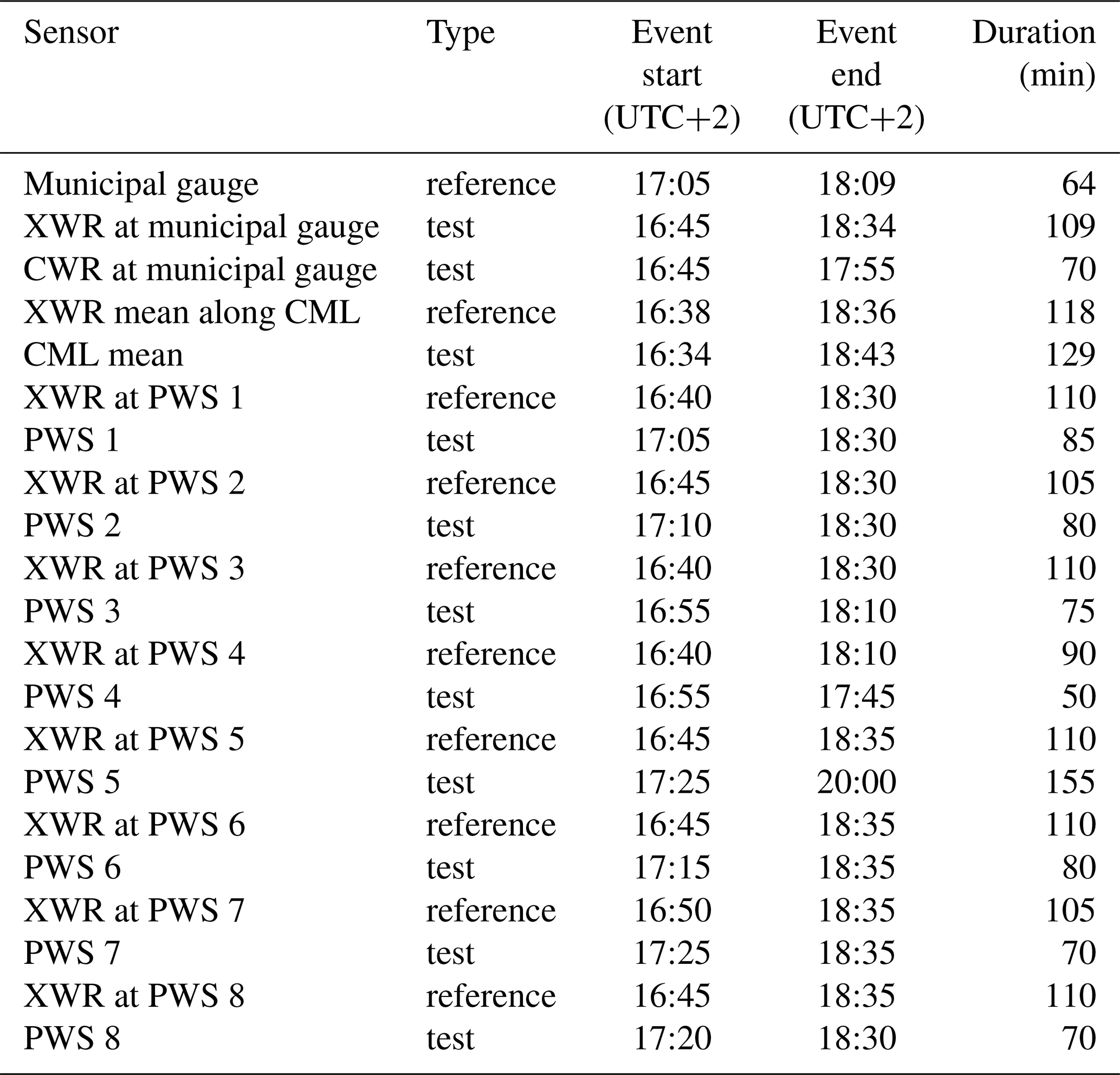
The PWS are concentrated in two clusters. PWS 1–4 are located in the western and central part of Båstad together with the municipal gauge, and PWS 5–8 in the north-eastern part (Fig. 1). In Table 2, it can be seen that ground observations in the mid-western part of Båstad started recording rain between 16:55 and 17:15 UTC+2, and the north-eastern part between 17:15 and 17:25 UTC+2, which suggests a gradual motion of the storm from west/south-west to the north-east. A similar tendency is seen in the XWR data, but with approximately 30 min time lag.

Figure 5Total accumulated depth (mm) of the event recorded by the national monitoring network.
5.2.2 National monitoring network
The total rainfall depth observed by the national monitoring network is shown in Fig. 5. The CWR grid size is 2×2 km. The weather station Hallands Väderö A, situated 15 km west of Båstad, records accumulated values every 15 min but only observed a total volume of 0.4 mm on the day of the event. The other stations report daily accumulations between 06:00–05:59 UTC+2, amounting to a maximum depth of 14.2 mm at Hov. All observations from SMHI's gauges corresponded to a return period of less than 1 year (Olsson et al., 2019). The heaviest rainfall observed by CWR was concentrated in the south of the Båstad urban area, with a maximum total depth of 65 mm, which corresponds to a return period of around 400 years for a duration of 60 min (Olsson et al., 2019). The maximum recorded depth in the area of interest was 25 mm (to the south-east), which corresponds to a return period of 11 years for a duration of 60 min.
Figure 6 shows the rainfall event observed by the municipal gauge, compared with CWR sampled at the same location. CWR underestimated the total depth with 57 mm when compared with the gauge, which suggests that CWR could not quantify the magnitude of the event accurately. The CWR started to observe rain 20 min before the rain gauge. Different time lags were applied to the time series by iteration, and it was found that rs could be raised from 0.4 to 0.83 when adding a lag of 10 min to the CWR data.
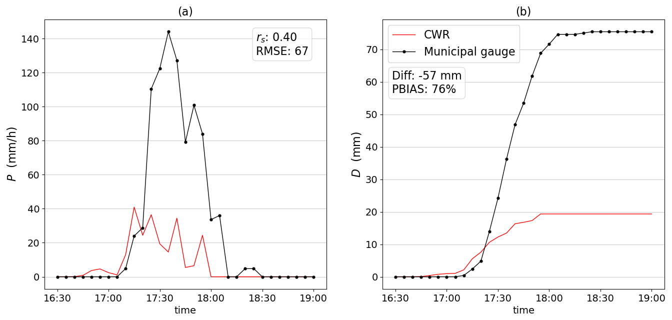
Figure 6(a) Rainfall intensity P (mm h−1), Spearman's rank coefficient rs (–) and RMSE (mm h−1). (b) Accumulated depth D (mm), difference in total depth and PBIAS. Evaluation metrics applied on CWR with municipal gauge as reference.
5.2.3 Second-party monitoring network
Figure 7 shows the total accumulated depth observed by the second-party network. The municipal gauge observed a total depth of 75.4 mm between 17:05 and 18:09 UTC+2, which is here approximated as 60 min. This corresponds to a return period of around 700 years (Olsson et al., 2019). The location of the heaviest rainfall was different when comparing gridded XWR data (250×250 m) to the CWR composite, where the XWR data indicated that the storm was centered just outside the coastline and not to the south of the Båstad urban area. The total depth of XWR sampled at the location of the municipal gauge based on the closest XWR bin was 78.4 mm, corresponding to a return period of around 800 years for 60 min duration, with observations up to almost 90 mm within the area of interest. XWR observations above 5 mm occurred over a much larger area compared with the CWR, especially to the north-east. This suggests that the CWR indeed was affected by beam blockage during the event as described in Sect. 3.1.
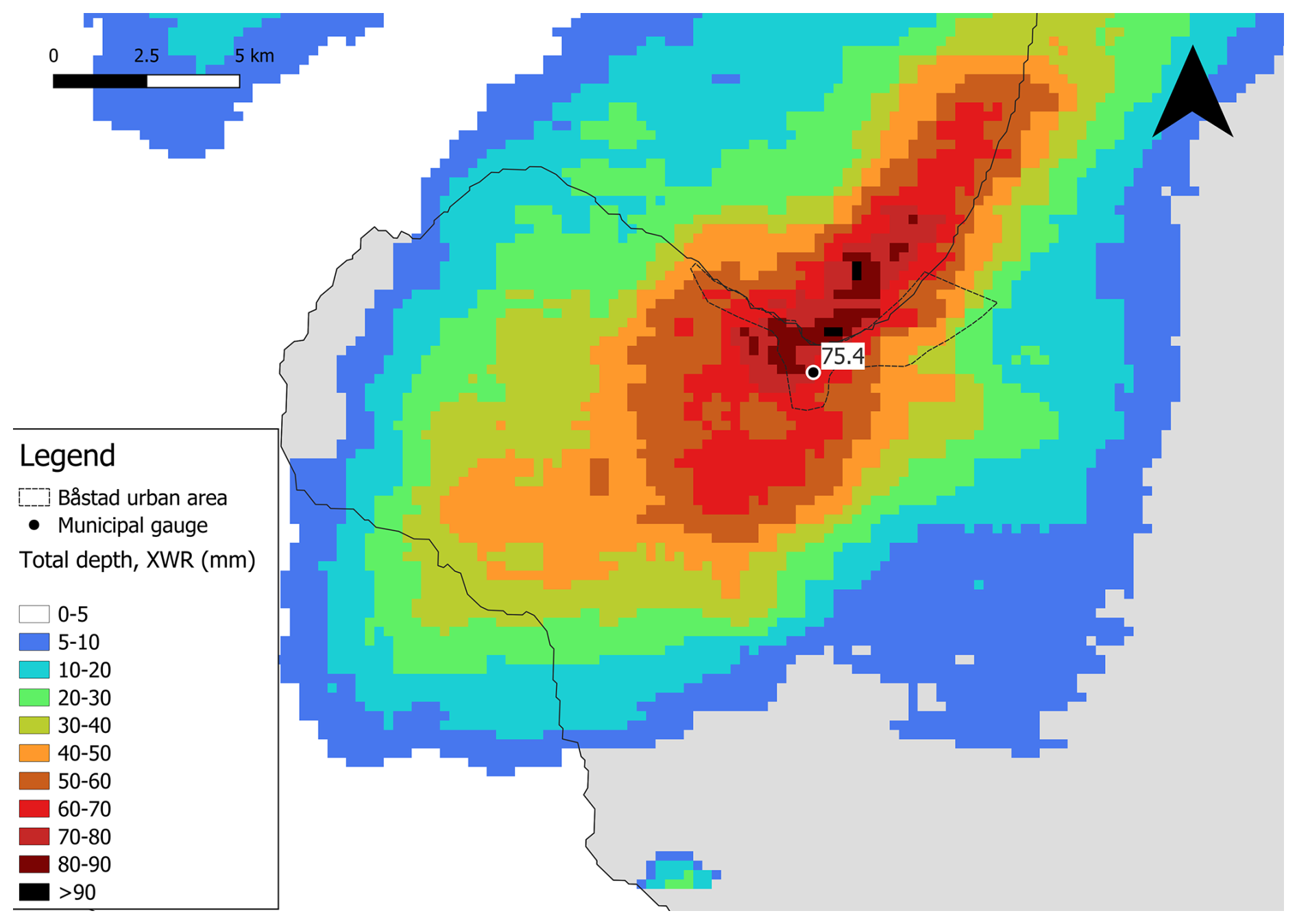
Figure 7Total accumulated depth (mm) of the event recorded by the second-party monitoring network.
Figure 8 shows the rainfall event observed by the municipal gauge, compared with XWR polar data sampled at the same location. As for CWR, the XWR started to record rain almost 20 min before the rain gauge. The correlation rs could be raised from 0.56 to 0.7 when adding a lag of 5 min to the XWR data. Even if the correlation was low with the reference, XWR observed a similar total depth with only 3 mm overestimation. In Fig. 8a, there is a tendency for XWR to underestimate the overall peak rainfall intensity and to overestimate lower rainfall intensities. This might be related to signal attenuation during heavy rain and the higher sensitivity of XWR to drizzles or observations of melting particles during light rain.
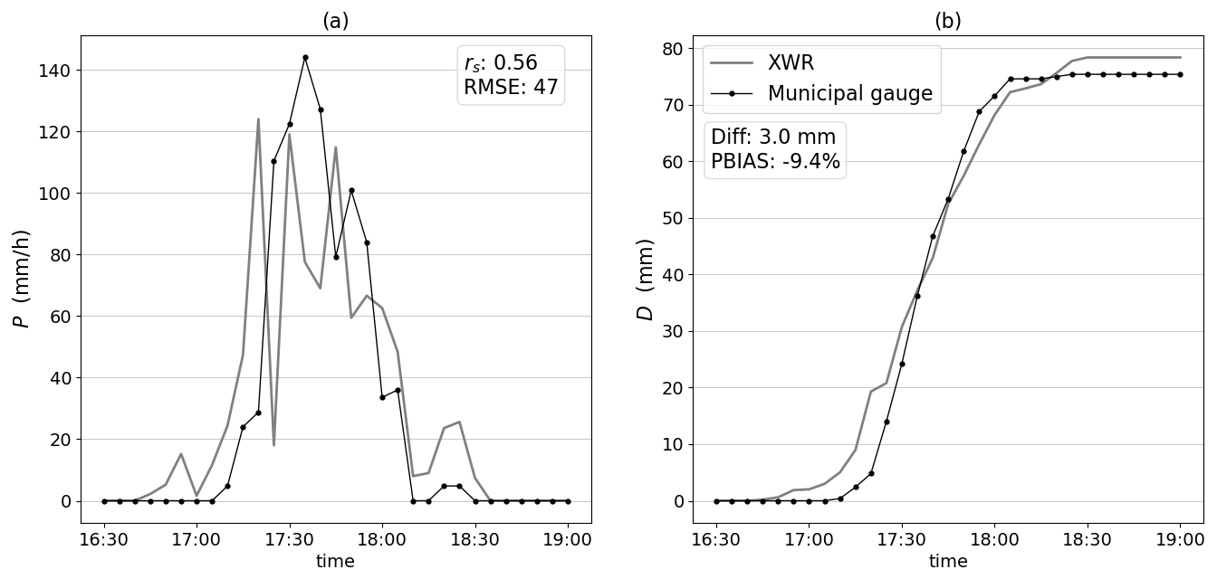
Figure 8(a) Rainfall intensity P (mm h−1), Spearman's rank coefficient rs (–) and RMSE (mm h−1). (b) Accumulated depth D (mm), difference in total depth and PBIAS. Evaluation metrics applied on XWR with municipal gauge as reference.
5.2.4 XWR and CML analysis along the CML path
Figure 9 shows the rainfall intensity PCML and depth DCML expressed as the mean of the two CML sub-links and the 10th–90th percentiles of the XWR bins sampled along each 250 m (amounting to 20 sample time series) along the CML path. The mean intensity of the XWR samples, PXWR, is highlighted in grey and was used as a reference for the CML. XWR on average started to observe rainfall at 16:38 UTC+2 along the link path, and CML at 16:43 UTC+2. PCML reached a “plateau” at 83 mm h−1 and stayed almost constant at this level for 31 min between 17:27–17:58 UTC+2. This effect is caused by the complete loss of radio signal between the CML base stations, which is induced by the heavy rainfall, as described by Blettner et al. (2023) and Polz et al. (2023). Likely by coincidence, CML recorded a similar total depth as the reference during the event, leading to a relatively small PBIAS. The large spread of 10–90th percentiles obtained from the 20 XWR observations suggests a large spatial variability of rainfall along the link.

Figure 9(a) Rainfall intensity P (mm h−1) of CML (mean) and XWR (mean and 10th to 90th percentile) along CML path. Spearman's rank coefficient rs (–) and RMSE (mm h−1). (b) Accumulated depth D (mm) of CML (mean) and XWR (mean and 10th to 90th percentile) along CML path. Difference in total depth and PBIAS. Evaluation metrics applied on CML mean with XWR mean as reference.
By inspecting radar fields, it was observed that the storm propagated almost perpendicularly over the CML link, which is favorable for a detailed comparison between the XWR and CML observations over the link path. Given the sudden constant records of rainfall rate observed in the CML time series, which are clearly not representative of the actual rainfall rate, the CML plateau period was considered unsuitable for the comparison. Instead, the following analysis focused on the periods right before and after the signal loss, from 16:38–17:26 and 17:59–18:36 UTC+2, for a total of 85 min.
Figure 10 shows the rainfall intensity distribution along the CML as observed by XWR for 5 min before and after the plateau. The first bin to the left in the plots was sampled at the western end of the CML, approximately 3.4 km away from the municipal gauge, and the last bin to the right was sampled at the eastern end, 1.6 km away from the gauge (see Fig. 1). The XWR sampling points closest to the rain gauge (bins 14 and 15, counting from the left) are at approximately 700 m distance from the gauge. PCML and Pmunicipal are also shown for each time step. The XWR spatial distribution was sometimes rather smooth, with a gradual increase and decrease along the link (e.g., Fig. 10b), but sometimes more intermittent, with large differences between adjacent XWR samples (e.g., Fig. 10g). In the pre-plateau period (Fig. 10a–e) PCML<PXWR consistently, whereas in the post-plateau period the relation was generally the opposite (Fig. 10f–j).
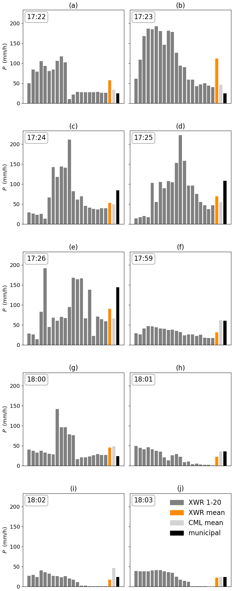
Figure 10(a–e) Rainfall intensity 5 min before CML signal loss (17:22–17:26 UTC+2). (f–j) Rainfall intensity 5 min after signal loss (17:59–18:03 UTC+2). Twenty radar bins sampled along CML path every 250 m (XWR 1–20), XWR mean, CML mean and municipal gauge.
The relationship between PXWR and PCML is shown for all observations in the pre- and post-plateau periods (in total 85 data points) in Fig. 11a. PCML was generally lower, and especially when PXWR<20 mm h−1, then PCML was consistently very low. This suggests that XWR is more sensitive to light rain than CML, as was observed when comparing with the municipal gauge (Sect. 5.2.3). Hypothesizing that the difference between PXWR and PCML was related to the XWR variability over the link, Fig. 11b shows the difference as a function of the X-band standard deviation σXWR. Despite a substantial scatter, a reasonably linear trend is suggested (R2=0.31) with PCML gradually underestimating more as the standard deviation increases.
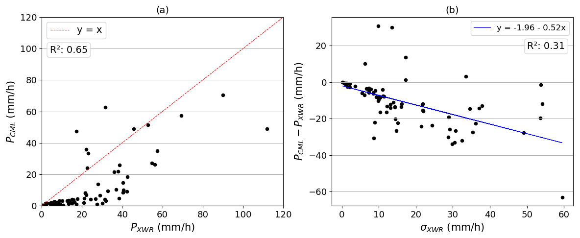
Figure 11(a) Mean rainfall intensity P (mm h−1) along the CML link as estimated by CML and XWR observations for 85 timesteps, before and after the plateau. (b) Difference between CML and XWR mean intensity values as a function of XWR standard deviation σXWR along the CML link.
5.2.5 Personal weather stations
This section starts with the results of the PWS quality control, before presenting the event observations. No faulty zeros or high influxes were detected during the event at any of the eight PWS in the area of interest. Three of the PWS – PWS 1, PWS 3 and PWS 4 – were flagged as station outliers. Nevertheless, all PWS were considered for further analysis to compare the output of the PWS quality control with traditional evaluation metrics. The eight PWS had between 25 and 29 stations within a 10 km radius that were included in the neighboring checks.
The PWS time series were also checked for the full year 2022. PWS 1 and 4 were flagged as faulty zeroes continuously during the winter months but had no Faulty Zero flags during the summer months (see Appendix A3, Fig. A2). The other PWS got intermittently flagged, but overall, there were few Faulty Zero flags during the year. No high influxes were detected at any PWS during 2022. All stations were flagged as Station Outliers during extended periods throughout the year, except one (PWS 6), which only had a few Station Outlier flags in December 2022 (see Appendix A3, Fig. A3).
Figure 12 shows the rainfall intensity P (mm h−1) observed by the eight PWS and XWR sampled at the PWS location, with metrics calculated with XWR as reference. The correlation with XWR was generally quite high, above 0.7 for five of the eight PWS. The CWR sampled at the PWS locations is included for comparison. Note that the CWR time series are identical for PWS 1 and 2, PWS 3 and 4, and PWS 6, 7 and 8 respectively, meaning that the PWS are situated in the same CWR grid cell.
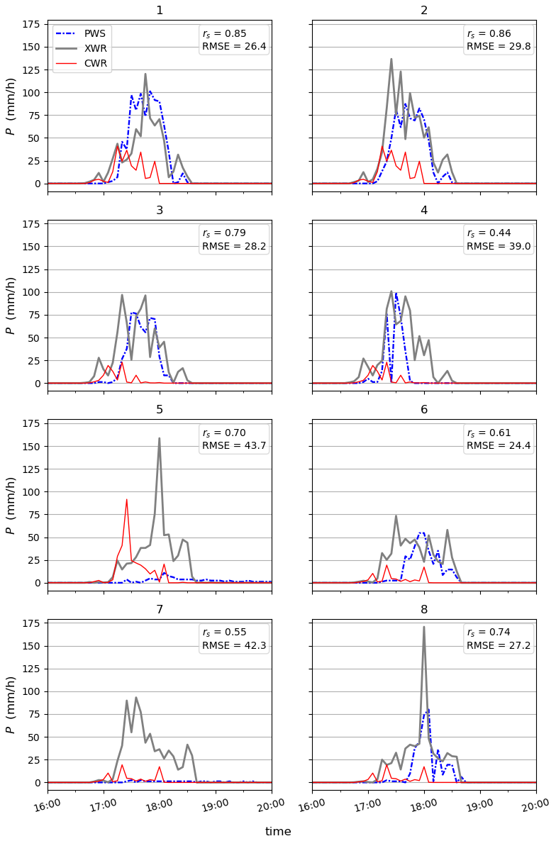
Figure 12Rainfall intensity P (mm h−1) for PWS 1–8. Spearman rank coefficient rs (–) and RMSE (mm h−1) calculated with XWR sampled at each PWS as reference. CWR sampled at each PWS included for comparison.
Figure 13 shows the accumulated rainfall depth D (mm) for the event. Almost all PWS significantly underestimated the total depth compared with the XWR reference. However, the estimate was closer to the reference compared with CWR, with two exceptions (PWS 5 and PWS 7). PWS 1 is the only PWS that overestimated compared with the reference, in total 7.7 mm (PBIAS −12.43 %).
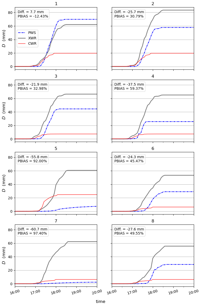
Figure 13Accumulated depth D (mm), difference in total depth and PBIAS calculated for PWS 1–8 with XWR sampled at each PWS as reference. CWR sampled at each PWS included for comparison.
This study investigates the capacity of second- and third-party sensors to observe short-duration extreme rainfall, compared with a conventional rainfall monitoring network. Sweden's national rainfall monitoring network, composed of automatic and manual weather stations and a CWR composite, is used as a conventional network in the study. The second-party network consists of a municipal rain gauge and an XWR operated by a local water utility company. CML and PWS are studied as third-party sensors. First, a long-term analysis of the municipal gauge is performed by cross-referencing two years of data with the national monitoring network. In this way, the municipal gauge is established as a trusted reference sensor for the study. Then, a convective rainfall event that hit southwestern Sweden in the late afternoon of 18 August 2022 is selected as a case study. The event analysis focuses on the urban area of Båstad, a small seaside municipality on the coast of Laholm Bay, as this location was particularly affected according to media reports.
No weather station in the national monitoring network captured the magnitude of the event as reported by the media (Sect. 5.2.2). The rainfall observed by the automatic and manual weather stations during the day of the event corresponded to a return period of less than one year, which suggests that the rainfall fell between the stations. CWR recorded a maximum total depth of 65 mm corresponding to a return period of 400 years, but the observation was made south of the Båstad urban area (Fig. 5). Within the area of interest, the maximum recorded depth was only 25 mm, which does not align with the municipal observations and the media reports about flooded streets and buildings.
CWR peaked at 92 mm h−1 at 17:25 UTC+2 in the sampling point at PWS 5, which is the only CWR observation in the expected magnitude of the event based on the municipal gauge. The specific CWR used in the study (location Ängelholm) is known to be affected by partial beam blockage which likely caused the severe underestimation (Appendix A1). This suggests that the siting of the radar should be improved, for example by vegetation clearance, increasing the height of the radar tower or relocation, to allow for better rainfall estimates. The underestimation may also be attributed to, for example, a lack of dual-polarization variables, insufficient attenuation correction (Hosseini et al., 2020), radar calibration or ground clutter removal (van de Beek et al., 2016). Furthermore, the use of the traditional Z–R (reflectivity – rain rate) relationship based on Marshall-Palmer coefficients (Marshall and Palmer, 1948) in the CWR data processing may not be well suited for convective storms. SMHI is currently developing new Z–R relationships for different weather conditions to improve the accuracy of CWR-based precipitation estimates in the future.
When turning to the second-party data, the magnitude of the event is starting to emerge. The municipal gauge showed good agreement with the national monitoring network in the long-term analysis and observed a ∼700-year rainfall in the Båstad urban area during the event (Sect. 5.2.3). The XWR sampled at the location of the municipal gauge recorded a total depth of 78.4 mm, corresponding to a return period of ∼800 years. It must be emphasized that estimated long return periods are highly dependent on the estimated rainfall duration, which may vary significantly in space and are difficult to firmly determine (Sect. 5.2.1). Furthermore, return period estimates are highly uncertain and should therefore not be quantified with high precision. In this context, a difference of ∼100 years must be considered relatively small and rather indicates a good agreement between the estimates.
XWR could accurately estimate the total rainfall depth compared with the municipal gauge (PBIAS 9.4 %). However, both radars showed a relatively low correlation with the reference; 0.56 for XWR (Fig. 8) and 0.4 for CWR (Fig. 6). The low correlation may be due to differences in the observation height between radar and gauge measurements. This could partly be accounted for by applying time lags and shifting the time series 5 and 10 min respectively, but also highlights the importance of accurate time stamping in the context of convective rainfall measurements.
XWR observations, particularly at long ranges, are known to be affected by signal attenuation due to interactions with hydrometeors (Bobotová et al., 2022; Lengfeld et al., 2016). However, XWR performed well during this event at a 40 km range, likely because the event occurred locally under a mostly clear sky. Remarkably, there was no intervening precipitation between the radar and the target area. Furthermore, it is perceived that beam overshooting was unlikely due to the higher altitude of summer precipitation compared to the XWR sampling volume at the lowest elevation angle.
One CML with a length of 4.8 km is located in the area of interest. The CML observed a similar duration of the event as the XWR reference (Sect. 5.2.4). The correlation was spuriously high (0.9) due to lack of variation in the CML rainfall rate, as it reached a `plateau' and stayed constant at this level for about 30 min, leading to an underestimation of the total depth. This effect is sometimes referred to as “blackout” (Polz et al., 2023) and appears when the radio signal is completely attenuated by heavy rainfall (ITU-R, 2005). Telecom network providers design the CML hardware so that transmission outages are allowed to occur 0.01 % of the time on an annual basis. Indeed, Polz et al. (2023) found that blackout gaps were present in less than 1 % of attenuation data from 4000 CMLs over 3 years in Germany, and that the effect on long-term timescales was generally low. However, the probability of a blackout at rainfall intensities above 100 mm h−1 was above 40 %, which implies that the CML technology currently has limitations in quantifying extreme events.
The analysis of XWR data along the CML link revealed some notable results. Firstly, the XWR data at some time steps exhibited a large bin-to-bin variability, sometimes shifting from one intensity level to another (Fig. 10b). This can be attributed to the turbulent nature of convective storms, and local attenuations of XWR signals during heavy rain bursts due to possible uncertainties in the attenuation correction. Despite overall agreement between PXWR and PCML along the link, a substantial scatter was found where, in particular, low intensities were consistently higher in the XWR data than CML (Fig. 11). Generally, there was a clear indication that the CML underestimation increased with increasing rainfall intensity as well as variability along the link. Berne and Uijlenhoet (2007) and de Vos et al. (2018) showed that spatial variability of rainfall can significantly affect CML-based rainfall estimates. A systematic underestimation of CML is expected for α<1 (see Appendix A2, Eq. A2) (Leijnse et al., 2010). Notably, the estimations of the event duration based on radars and CML were significantly different from the in-situ gauge observations. For example, the municipal gauge started to observe the event 20 min after CWR. These discrepancies could be attributed to the larger sensitivity of CML and radars to light rainfall and slow accumulations in the tipping-bucket gauge during light drizzles preceding the heavy bursts.
Regarding the eight PWS in the area of interest, the tipping bucket mechanism seems to have reached a maximum tipping frequency (i.e., detectable intensity) during the highest-intensity periods, as no observation exceeded 100 mm h−1 (Fig. 12). A similar tendency has been observed by others (Lussana et al., 2023; Wolf and Larsson, 2024). Among the PWS with lowest RMSE, this led to a PBIAS of 30 %–40 % compared with the XWR reference (Fig. 13). PWS 1 performed reasonably well on all evaluation metrics with a Spearman correlation of 0.85, RMSE 26.4 mm h−1 and PBIAS −12.4 %. In most cases, the correlation with reference was medium to high, with only two PWS (PWS 4 and 7, Fig. 12) having a correlation below 0.6.
We applied a quality control specifically designed for PWS rainfall data, pypwsqc ( ) (Graf et al., 2025) on the event and full year 2022 (Sect. 5.2.5). The algorithm applies three filters – Faulty Zeroes filter, High Influx filter, and Station Outlier filter – to assess the quality of each time step by utilizing neighbor checks with nearby stations. No faulty zeroes were detected during the event, which is reasonable as all PWS in the area of interest measured rainfall at all timesteps. No high influxes were found, suggesting that all PWS in the area measured enough rainfall not to trigger high influx flags at the neighboring stations. On the other hand, no high influx was detected at any PWS during the entire year 2022. There might indeed not have been any high influx recorded by any of the 58 PWS on the Bjäre Peninsula in 2022, but the results also raise the question of whether the filter parameters should be tuned differently to better capture unrealistically high inflows.
Regarding the Station Outlier filter, three stations were flagged as station outliers during the event – PWS 1, PWS 3 and PWS 4. However, when inspecting the time series and evaluation metrics for these stations, it appeared that PWS 1 and PWS 3 had among the highest correlations and lowest RMSE of all PWS and generally showed a reasonable rainfall pattern compared with the other PWS (Fig. 12). These results point to a limitation of neighboring checks in the context of convective storms. PWS 1, PWS 3 and PWS 4 are all located in the western part of Båstad. As such, the Station Outlier filter considered the observations of PWS located further to the west on the Bjäre Peninsula, which experienced a total depth of only 10 mm according to the XWR observations. The high spatial variability of the event therefore triggered station outlier flags at the three PWS located closest to the drier area, even if two of them performed well when compared with the XWR reference.
The parameter settings suggested in literature (Sect. 4.4) (de Vos et al., 2019) were changed in the Station Outlier filter. However, it is not expected that the changes created these results as the filter would not have been possible to apply at all for the event with the original numbers as there were too few wet time steps in the weeks preceding the storm. If the flagged PWS had been removed from further analysis based on the results from the Station Outlier filter, sound observations would have been lost. Conversely, the performance of PWS 5 and PWS 7 was very poor compared with the XWR reference, but these stations were not flagged in the automatic quality control. Future research should explore how the spatial density of PWS and the considered evaluation range influence the capability of neighbor checks to be applicable as quality control protocols for localized rainfall.
The findings of this study align with the well-established fact that conventional monitoring networks have limitations in terms of observing convective rainfall. To strengthen capacity in this field, NMHS can include second-party data in operational tools and workflows. However, differences in acquisition protocols, data formats etc. adopted by different actors may cause an additional burden and hinder the integration of second-party sensors. Importantly, Skåne County has an excellent coverage of second-party sensors thanks to the combination of XWR and rain gauges operated by local authorities, which is certainly not the case for all points of interest, particularly in countries with limited resources (Winsemius et al., 2018). In those cases, NMHS can turn to third-party sensors, particularly CML that are typically available in populated settlements across the globe (Chwala and Kunstmann, 2019; Blettner et al., 2023). However, the results of this study suggest that these sensors currently have limitations in quantifying the correct magnitude of convective storms. Still, the results show that third-party data may assist in detecting storm durations and the spatial distribution of rainfall.
Regarding limitations of the study, a few remarks can be made. First, there are uncertainties associated with all observations in the study, especially the indirect rainfall measurements (radars and CML) and the PWS. The long-term assessment of the municipal gauge, combined with the good agreement between the municipal gauge and XWR, still provide solid evidence for the actual magnitude of the event. Secondly, some findings are expected to be specific for this study, such as the low performance by CWR caused by beam blockage in the area of interest. On the other hand, the underestimation of rainfall observed by the third-party network aligns with previous studies. It is also expected that quality control protocols that utilize neighboring checks will be problematic for other convective storms, depending on the station network density and considered range of the analysis. Although no general conclusions can be drawn from a case study, we believe that the depth of this analysis contributes to the understanding of advantages and limitations when observing convective rainfall with second- and third-party sensors.
This study investigated the capacity of second- and third-party sensors to observe short-duration extreme rainfall compared with a conventional rainfall monitoring network in a case study. The results show that the conventional network underestimated the total rainfall depth of the event and was unable to fully capture the extreme spatial variability of the convective storm. Only when considering observations from second- and third-party sensors, more accurate representations of the magnitude and spatial extent of the storm could be obtained, which suggests that NMHS could utilize these sensors to improve observations of convective rainfall. However, second-party sensors are not always available, particularly in resource-strained settings. Furthermore, the results suggest that third-party sensors can assist in detecting storm durations and spatial variability of rainfall but have limitations in quantifying the correct magnitude of convective storms. Third-party data may also be difficult to obtain for NMHS and has known problems with data quality. Future research is suggested to continue the efforts on quality control of third-party data, especially related to extreme events. In addition, more research is needed on the integration of second- and third-party data in the workflows of NMHS.
A1 Vegetation affecting the Ängelholm radar location
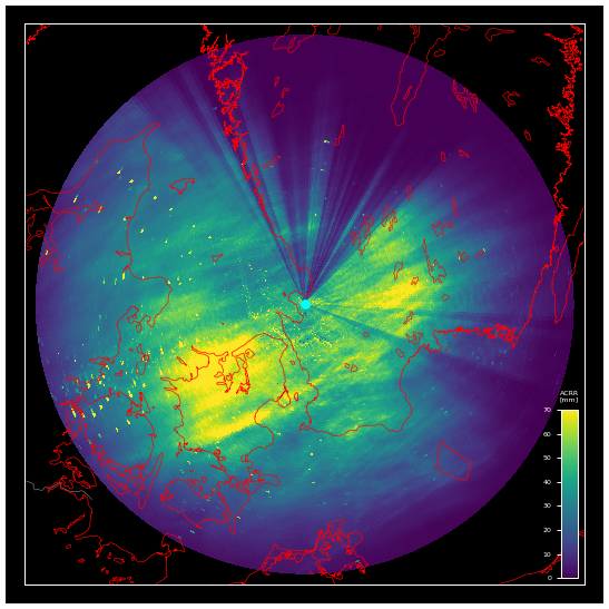
The Ängelholm radar location is affected by partial beam blockage in a circular sector of around 60° to the North (Fig. A1) (SMHI, 2025a). Båstad is located 6 km to the north of the radar. The figure shows accumulated precipitation detected by the radar during the period 3–17 October 2019. Darker color indicates less total precipitation.
The partial beam blockage is caused by vegetation within 1 km north of the radar location. Figure A2 shows the Ängelholm radar beam in the north direction overlaid with a point cloud of vegetation based on aerial laser scans (Lantmäteriet, 2025). Note that the figure reflects the status as of 2019 and the vegetation has likely grown taller since.
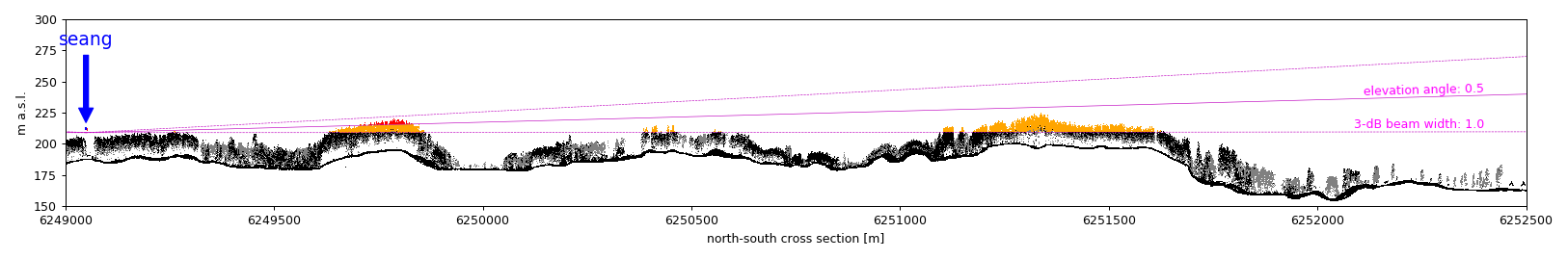
Figure A2Ängelholm radar beam in the north direction overlaid with a point cloud of vegetation based on aerial laser scans (Lantmäteriet, 2025).
A2 CML processing
When estimating rainfall intensity from CML data, the first step is to identify a link-specific threshold for classification of wet and dry timesteps. The challenge is to detect small rainfall volumes (true wet periods) without including too many dry periods with strong attenuation from other causes, such as changes in water vapor content or air temperature (false wet periods). Several approaches have been suggested in literature (Rayitsfeld et al., 2012; Wang et al., 2012; Cherkassky et al., 2014; Overeem et al., 2016). Schleiss and Berne (2010) proposed a simple classification method that considers the rolling standard deviation of the attenuation, assuming that the variability is small during dry periods and large during wet periods. The time step is classified as dry if the variability falls below a defined threshold value, which must be calibrated with secondary observations nearby the link. More recently, machine learning approaches has shown strong potential to effectively classify wet and dry timesteps in CML data (Habi and Messer, 2018; Polz et al., 2020; Øydvin et al., 2024).
The second step is to define a “baseline level”, that is, RSL during dry weather. This is used as the reference level for the rain attenuation calculation and is typically based on the signal attenuation during dry time steps preceding a wet period (Andersson et al., 2022). In addition, the signal is often corrected for additional attenuation caused by water on the cover of the antenna, so-called “wet antenna attenuation” (e.g., Leijnse et al., 2007a, 2008; Graf et al., 2020). Finally, the corrected attenuation is converted into rain rate using an inverted power law relationship. The MEMO method was developed and tested on an open data set (“OpenMRG”) that consists of 364 CML and 11 rainfall gauges in Gothenburg, Sweden, for the period June–August 2015 (Andersson et al., 2022). The processing steps of the MEMO methodology are outlined below.
A2.1 Data pre-processing
The 10 s attenuation was calculated by taking the difference between TSL and RSL. Then, the median value over a 1 min period Aml was taken for all minutes that had more than four 10 s values in 1 min and if less data were available, that minute was flagged as missing data.
A2.2 Wet-dry classification
Sub-links in the OpenMRG dataset were scrutinized to find a wet-dry classification method that does not rely on secondary observations. The links considered were located within 500 m from a municipal rain gauge in Gothenburg that records at 1 min temporal resolution, resulting in 72 links. First, dry time steps recorded by the station between 14 May to 31 August 20151 were considered. A time buffer of 30 min was added before and after each rain event recorded by the rain gauge, to consider that rainfall arrives at different timesteps to the links. The 99th percentile of Aml at dry timesteps identified by the rain gauge was considered to address that the links may record rainfall that was missed by the rain gauge. Then, the empirical distribution of Aml at the dry timesteps was plotted and inspected for the 72 links. An example is shown in Fig. A3. In this example, the difference between the median and 99th percentile of the attenuation is 0.35 dB.

Figure A3Example of empirical distribution of attenuation level (Aml) at dry timesteps for Link 312.
The plots showed that the difference in Aml between the median attenuation and the 99th percentile was typically between 0.35–0.6 dB at dry timesteps. However, the difference for one link with considerable fluctuations in signal attenuation was 1.7 dB. Based on these results, it was decided to set the threshold for the wet-dry classification to the median attenuation over the past 2 weeks plus an additional 1.7 dB (here called the “median buffer method”). In this study, where only two days of data was available, the median was taken over all available preceding time steps.
The median buffer method was compared with classifying all timesteps with attenuation above the median of the last two weeks as wet (“median method”) and the method presented by Schleiss and Berne (2010) (“Schleiss method”). The median method resulted in overestimation of the number of wet timesteps compared with the rain gauge. The Schleiss method performed similarly to the median buffer method in correctly identifying the number of wet timesteps but resulted in some outliers and produced more false wet time steps. Based on these results, the median buffer method was used for further analysis.
A3 Baseline definition
The baseline Abl is the expected difference between TSL and RSL during dry weather. This means that during dry periods, based on the wet-dry classification in the previous step, the baseline is equal to the attenuation Aml. During wet periods, the baseline is taken as the median of the last N timesteps from the first wet timestep. A suitable reference period for N was found to be 240 min.
A4 Conversion of net attenuation to rain rate
By subtracting the baseline from the attenuation, the net attenuation Anl was found as
Following common practice in CML literature (Leijnse et al., 2007b; Messer et al., 2006), specific attenuation (dB km−1) was converted to rain rate (Praw) using link length (L, km) and the power–law relationship:
The parameters k and α depend on link frequency, the polarization state, and the elevation angle of the signal path and was found by applying the equations derived by ITU-R (2005). For the link in this paper, k=0.13 and α=0.96 (23.1 GHz, vertical polarization). In contrast to radar scatter, the sensitivity to DSD (Eq. 1) is very limited around 30 GHz because α is approximately 1 in this range, suggesting a nearly linear relation between net attenuation and rain rate (Chwala and Kunstmann, 2019). At frequencies further from 30 GHz, DSD will play a larger role and biases can occur. Most links in Sweden operate near 30 GHz (Andersson et al., 2022).
A5 Bias correction based on link length
The derived rain rate was analyzed for the 72 links situated within 500 m range from the 11 rain gauges in the OpenMRG dataset for July 2015. When plotting the residuals of the rain rate at the closest gauge against 15 min accumulated net attenuation of the link, a linear relationship was found, indicating potential for bias correction. The slope of the residuals was derived by linear regression for each link and plotted against the link frequency, link length and the parameters k and α in Eq. (A2). The most distinct relationship was found for link length, suggesting that the shorter the length, the higher the slope of the residuals. One probable reason for the relationship is the wet-antenna effect, which is stronger over shorter distances (Chwala and Kunstmann, 2019).
It was found that the slope of the regression line of the residuals could be estimated from link length by applying a simple inverse equation:
where L is the link length. The parameters f, g, and h were optimized by minimizing the Mean Absolute Error for the 72 links, arriving at 2.85214, 1.672 and 0.1615, respectively. The bias corrected rain rate for the CML in Båstad was then found by calculating the correction factor:
where L is 4.8 km in this case. Then, applying the factor to the derived rain rate:
A6 PWS quality control 2022
Figure A4 shows Faulty Zero (FZ) flags for the eight PWS in the area of interest for the full year 2022.
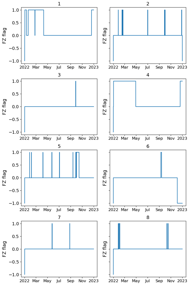
Figure A4Faulty Zero (FZ) flags 2022. 1 = FZ flag, 0 = no FZ-flag, −1 = FZ-filter could not be applied.
Figure A5 shows Station Outlier (SO) flags for the eight PWS in the area of interest for the full year 2022.
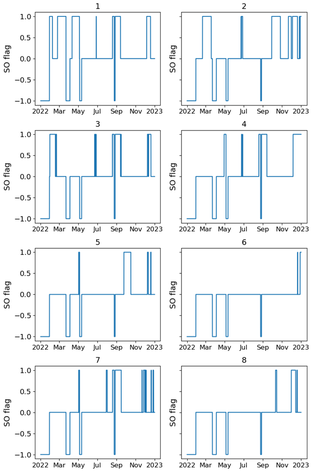
National weather station data and C-band radar composite are available from SMHI's open data archive (https://www.smhi.se/data, last access: 12 January 2026). The processed national data are available on request. Data from the municipal gauge and X-band radar is the property of Nordvästra Skånes Vatten och Avlopp, NSVA. CML data is the property of the telecom companies Ericsson AB and Tre. PWS data is the property of Netatmo. However, Netatmo data can be openly accessed through their API: https://weathermap.netatmo.com (last access: 12 January 2026).
LPW processed gauge data. LPW and RvdB processed CWR data. HaH, LPW and RvdB processed XWR data. RvdB and LPW processed CML data. JA developed the CML processing methodology. LPW implemented the PWS quality control. LPW, JO and HaH performed data analysis. All authors were involved in the writing and editing of this manuscript.
The contact author has declared that none of the authors has any competing interests.
Publisher's note: Copernicus Publications remains neutral with regard to jurisdictional claims made in the text, published maps, institutional affiliations, or any other geographical representation in this paper. The authors bear the ultimate responsibility for providing appropriate place names. Views expressed in the text are those of the authors and do not necessarily reflect the views of the publisher.
The authors would like to thank NSVA for sharing tipping bucket data and Ericsson AB and Tre for sharing CML data. Lennart Simonsson processed PWS data to NetCDF-files. Riejanne Mook improved the CML processing code. Daniel Johnson provided information on the partial beam blockage of the Ängelholm C-band radar.
The paper was supported by the Swedish Research Council Formas through the projects SPARC (Stakeholder participation for climate adaptation – data crowdsourcing for improved urban flood risk management, grant 2021-02380 Formas) and HyPrecip (Hyper-resolution multidimensional precipitation information for analysis and modelling: urban and rural applications, grant 2021-01629 Formas). The development of pypwsqc received funding from the European Union's Framework Programme for Research & Innovation as part of the COST Action OpenSense [CA20136], as supported by the COST Association (European Cooperation in Science and Technology).
The publication of this article was funded by the Swedish Research Council, Forte, Formas, and Vinnova.
This paper was edited by Gianfranco Vulpiani and reviewed by Hidde Leijnse and one anonymous referee.
Andersson, J. C. M., Olsson, J., van de Beek, R. (C Z.), and Hansryd, J.: OpenMRG: Open data from Microwave links, Radar, and Gauges for rainfall quantification in Gothenburg, Sweden, Earth Syst. Sci. Data, 14, 5411–5426, https://doi.org/10.5194/essd-14-5411-2022, 2022.
Bárdossy, A., Seidel, J., and El Hachem, A.: The use of personal weather station observations to improve precipitation estimation and interpolation, Hydrol. Earth Syst. Sci., 25, 583–601, https://doi.org/10.5194/hess-25-583-2021, 2021.
Båserud, L., Lussana, C., Nipen, T. N., Seierstad, I. A., Oram, L., and Aspelien, T.: TITAN automatic spatial quality control of meteorological in-situ observations, Adv. Sci. Res., 17, 153–163, https://doi.org/10.5194/asr-17-153-2020, 2020.
Battan, L. J.: Radar Observation of the Atmosphere, Rev. Edn., University of Chicago Press, https://doi.org/10.1002/qj.49709942229, 1973.
Bengtsson, L.: Regn i Båstad, Vatten Tidskr, För Vattenvård J. Water Manag. Res., 1–2, 61–70, 2023.
Berne, A. and Uijlenhoet, R.: Path-averaged rainfall estimation using microwave links: Uncertainty due to spatial rainfall variability, Geophys. Res. Lett., 34, https://doi.org/10.1029/2007GL029409, 2007.
Blettner, N., Fencl, M., Bareš, V., Kunstmann, H., and Chwala, C.: Transboundary rainfall estimation using commercial microwave links, Earth Space Sci., 10, e2023EA002869, https://doi.org/10.1029/2023EA002869, 2023.
Bobotová, G., Sokol, Z., Popová, J., Fišer, O., and Zacharov, P.: Analysis of two convective storms using polarimetric X-band radar and satellite data, Remote Sens., 14, 2294, https://doi.org/10.3390/rs14102294, 2022.
Boonstra, M. M. T.: Delft Measures Rain. A quality assessment of precipitation measurements from personal weather stations, MS thesis, Delft University of Technology, the Netherlands, https://resolver.tudelft.nl/uuid:c5720b7e-1828-4948-a76a-89a6361b3e03 (last access: 12 January 2026), 2024.
Cherkassky, D., Ostrometzky, J., and Messer, H.: Precipitation classification using measurements from commercial microwave links, IEEE T. Geosci. Remote, 52, 2350–2356, https://doi.org/10.1109/TGRS.2013.2259832, 2014.
Chwala, C. and Kunstmann, H.: Commercial microwave link networks for rainfall observation: Assessment of the current status and future challenges, WIREs Water, 6, e1337, https://doi.org/10.1002/wat2.1337, 2019.
de Vos, L. W., Raupach, T. H., Leijnse, H., Overeem, A., Berne, A., and Uijlenhoet, R.: High-resolution simulation study exploring the potential of radars, crowdsourced personal weather stations, and commercial microwave links to monitor small-scale urban rainfall, Water Resour. Res., 54, 10293–10312, https://doi.org/10.1029/2018WR023393, 2018.
de Vos, L. W., Leijnse, H., Overeem, A., and Uijlenhoet, R.: Quality control for crowdsourced personal weather stations to enable operational rainfall monitoring, Geophys. Res. Lett., 46, 8820–8829, https://doi.org/10.1029/2019GL083731, 2019.
Einfalt, T., Arnbjerg-Nielsen, K., Golz, C., Jensen, N.-E., Quirmbach, M., Vaes, G., and Vieux, B.: Towards a roadmap for use of radar rainfall data in urban drainage, J. Hydrol., 299, 186–202, https://doi.org/10.1016/j.jhydrol.2004.08.004, 2004.
Fencl, M., Nebuloni, R., C. M. Andersson, J., Bares, V., Blettner, N., Cazzaniga, G., Chwala, C., Colli, M., de Vos, L., El Hachem, A., Galdies, C., Giannetti, F., Graf, M., Jacoby, D., Victor Habi, H., Musil, P., Ostrometzky, J., Roversi, G., Sapienza, F., Seidel, J., Spackova, A., van de Beek, R., Walraven, B., Wilgan, K., and Zheng, X.: Data formats and standards for opportunistic rainfall sensors, Open Res. Eur., 3, 169, https://doi.org/10.12688/openreseurope.16068.2, 2024.
Foreningen VeVa: Vejrradar i vandsektoren, https://veva.dk/ (last access: 19 May 2025), 2025.
Fuentes-Andino, D., Beven, K., Halldin, S., Xu, C.-Y., Reynolds, J. E., and Di Baldassarre, G.: Reproducing an extreme flood with uncertain post-event information, Hydrol. Earth Syst. Sci., 21, 3597–3618, https://doi.org/10.5194/hess-21-3597-2017, 2017.
Garcia-Marti, I., Overeem, A., Noteboom, J. W., de Vos, L., de Haij, M., and Whan, K.: From proof-of-concept to proof-of-value: Approaching third-party data to operational workflows of national meteorological services, Int. J. Climatol., 43, 275–292, https://doi.org/10.1002/joc.7757, 2023.
Graf, M., Chwala, C., Polz, J., and Kunstmann, H.: Rainfall estimation from a German-wide commercial microwave link network: optimized processing and validation for 1 year of data, Hydrol. Earth Syst. Sci., 24, 2931–2950, https://doi.org/10.5194/hess-24-2931-2020, 2020.
Graf, M., Chwala, C., Petersson Wårdh, L., and Seidel, J.: OpenSenseAction/pypwsqc: v0.2.1, Zenodo [code], https://doi.org/10.5281/zenodo.16748098, 2025.
Gravlund: Hagel och regnkaos över Båstad: “Aldrig sett något liknande”, https://www.svt.se/nyheter/lokalt/helsingborg/kraftiga-skyfall-over-bastad-har-aldrig-varit-med-om-nagot-liknande (last access: 14 April 2025), 2025.
Guo, Y.: Updating Rainfall IDF Relationships to Maintain Urban Drainage Design Standards, J. Hydrol. Eng., 11, 506–509, https://doi.org/10.1061/(ASCE)1084-0699(2006)11:5(506), 2006.
Gupta, H. V., Sorooshian, S., and Yapo, P. O.: Status of automatic calibration for hydrologic models: comparison with multilevel expert calibration, J. Hydrol. Eng., 4, 135–143, https://doi.org/10.1061/(ASCE)1084-0699(1999)4:2(135), 1999.
Habi, H. V. and Messer, H.: Wet-dry classification using LSTM and commercial microwave links, in: 2018 IEEE 10th Sensor Array and Multichannel Signal Processing Workshop (SAM), Sheffield, UL, 149–153, https://doi.org/10.1109/SAM.2018.8448679, 2018.
Hahn, C., Garcia-Marti, I., Sugier, J., Emsley, F., Beaulant, A.-L., Oram, L., Strandberg, E., Lindgren, E., Sunter, M., and Ziska, F.: Observations from personal weather stations – EUMETNET interests and experience, Climate, 10, 192, https://doi.org/10.3390/cli10120192, 2022.
Hosseini, S. H., Hashemi, H., Berndtsson, R., South, N., Aspegren, H., Larsson, R., Olsson, J., Persson, A., and Olsson, L.: Evaluation of a new X-band weather radar for operational use in south Sweden, Water Sci. Technol., 81, 1623–1635, https://doi.org/10.2166/wst.2020.066, 2020.
Hosseini, S. H., Hashemi, H., Larsson, R., and Berndtsson, R.: Merging dual-polarization X-band radar network intelligence for improved microscale observation of summer rainfall in south Sweden, J. Hydrol., 617, 129090, https://doi.org/10.1016/j.jhydrol.2023.129090, 2023.
Hyndman, R. J. and Koehler, A. B.: Another look at measures of forecast accuracy, Int. J. Forecast., 22, 679–688, https://doi.org/10.1016/j.ijforecast.2006.03.001, 2006.
Imhoff, R. O., Brauer, C. C., Overeem, A., Weerts, A. H., and Uijlenhoet, R.: Spatial and temporal evaluation of radar rainfall nowcasting techniques on 1,533 events, Water Resour. Res., 56, e2019WR026723, https://doi.org/10.1029/2019WR026723, 2020.
ITU-R: Recommendation ITU-R P.838-3: Specific attenuation model for rain for use in prediction methods, Radiocommunication Sector of International Telecommunication Union, https://www.itu.int/rec/R-REC-P.838-3-200503-I/en (last access: 12 January 2026), 2005.
Kaiser, M., Günnemann, S., and Disse, M.: Spatiotemporal analysis of heavy rain-induced flood occurrences in Germany using a novel event database approach, J. Hydrol., 595, 125985, https://doi.org/10.1016/j.jhydrol.2021.125985, 2021.
Kumjian, M.: Principles and applications of dual-polarization weather radar. Part I: Description of the polarimetric radar variables, J. Oper. Meteorol., 1, 226–242, https://doi.org/10.15191/nwajom.2013.0119, 2013.
Lantmäteriet: Laserdata Nedladdning, skog, https://www.lantmateriet.se/sv/geodata/vara-produkter/produktlista/laserdata-nedladdning-skog (last access: 7 November 2025), 2025.
Leijnse, H., Uijlenhoet, R., and Stricker, J. N. M.: Hydrometeorological application of a microwave link: 2. Precipitation, Water Resour. Res., 43, W04417, https://doi.org/10.1029/2006WR004989, 2007a.
Leijnse, H., Uijlenhoet, R., and Stricker, J. N. M.: Rainfall measurement using radio links from cellular communication networks, Water Resour. Res., 43, https://doi.org/10.1029/2006WR005631, 2007b.
Leijnse, H., Uijlenhoet, R., and Stricker, J. N. M.: Microwave link rainfall estimation: Effects of link length and frequency, temporal sampling, power resolution, and wet antenna attenuation, Adv. Water Resour., 31, 1481–1493, https://doi.org/10.1016/j.advwatres.2008.03.004, 2008.
Leijnse, H., Uijlenhoet, R., and Berne, A.: Errors and uncertainties in microwave link rainfall estimation explored using drop size measurements and high-resolution radar data, J. Hydrometeorol., 11, 1330–1344, https://doi.org/10.1175/2010JHM1243.1, 2010.
Lengfeld, K., Clemens, M., Merker, C., Münster, H., and Ament, F.: A simple method for attenuation correction in local X-band radar measurements using C-band radar data, J. Atmos. Ocean. Tech., 33, 2315–2329, https://doi.org/10.1175/JTECH-D-15-0091.1, 2016.
Lewis, E., Pritchard, D., Villalobos-Herrera, R., Blenkinsop, S., McClean, F., Guerreiro, S., Schneider, U., Becker, A., Finger, P., Meyer-Christoffer, A., Rustemeier, E., and Fowler, H. J.: Quality control of a global hourly rainfall dataset, Environ. Model. Softw., 144, 105169, https://doi.org/10.1016/j.envsoft.2021.105169, 2021.
Lussana, C., Baietti, E., Båserud, L., Nipen, T. N., and Seierstad, I. A.: Exploratory analysis of citizen observations of hourly precipitation over Scandinavia, Adv. Sci. Res., 20, 35–48, https://doi.org/10.5194/asr-20-35-2023, 2023.
Mailhot, A. and Duchesne, S.: Design criteria of urban drainage infrastructures under climate change, J. Water Resour. Plan. Manage., 136, 201–208, https://doi.org/10.1061/(ASCE)WR.1943-5452.0000023, 2010.
Mandement, M. and Caumont, O.: Contribution of personal weather stations to the observation of deep-convection features near the ground, Nat. Hazards Earth Syst. Sci., 20, 299–322, https://doi.org/10.5194/nhess-20-299-2020, 2020.
Marchi, L., Borga, M., Preciso, E., Sangati, M., Gaume, E., Bain, V., Delrieu, G., Bonnifait, L., and Pogačnik, N.: Comprehensive post-event survey of a flash flood in Western Slovenia: observation strategy and lessons learned, Hydrol. Process., 23, 3761–3770, https://doi.org/10.1002/hyp.7542, 2009.
Marshall, J. S. and Palmer, W. M. K.: The distribution of raindrops with size, J. Atmos. Sci., 5, 165–166, https://doi.org/10.1175/1520-0469(1948)005<0165:TDORWS>2.0.CO;2, 1948.
MEMO: MEMO, https://www.smhi.se/en/research/about-us/open-access-to-data-for-research-and-development/memo (last access: 15 April 2025), 2025.
Messer, H., Zinevich, A., and Alpert, P.: Environmental monitoring by wireless communication networks, Science, 312, 713–713, https://doi.org/10.1126/science.1120034, 2006.
Michelson, D., Henja, A., Ernes, S., Haase, G., Koistinen, J., Ośródka, K., Peltonen, T., Szewczykowski, M., and Szturc, J.: BALTRAD Advanced Weather Radar Networking, J. Open Res. Softw., 6, 12, https://doi.org/10.5334/jors.193, 2018.
Michelson, D. B. and Koistinen, J.: Gauge-Radar network adjustment for the Baltic Sea experiment, Phys. Chem. Earth Pt. B, 25, 915–920, https://doi.org/10.1016/S1464-1909(00)00125-8, 2000.
Michelson, D. B., Lewandowski, R., Szewczykowski, M., Beekhuis, H., and Haase, G.: EUMETNET OPERA weather radar information model for implementation with the HDF5 file format, version 2.2, https://eumetnet.eu/wp-content/uploads/2017/01/OPERA_hdf_description_2014.pdf (last access: 13 January 2026), 2014.
Mobini, S., Nilsson, E., Persson, A., Becker, P., and Larsson, R.: Analysis of pluvial flood damage costs in residential buildings – A case study in Malmö, Int. J. Disast. Risk Reduct., 62, 102407, https://doi.org/10.1016/j.ijdrr.2021.102407, 2021.
Nielsen, J. M., van de Beek, C. Z. R., Thorndahl, S., Olsson, J., Andersen, C. B., Andersson, J. C. M., Rasmussen, M. R., and Nielsen, J. E.: Merging weather radar data and opportunistic rainfall sensor data to enhance rainfall estimates, Atmos. Res., 300, 107228, https://doi.org/10.1016/j.atmosres.2024.107228, 2024.
Olsson, J., Södling, J., Berg, P., Wern, L., and Eronn, A.: Short-duration rainfall extremes in Sweden: a regional analysis, Hydrol. Res., 50, 945–960, https://doi.org/10.2166/nh.2019.073, 2019.
Olsson, J., Horváth-Varga, L., Beek, R. van de, Graf, M., Overeem, A., Szaton, M., Bareš, V., Bezak, N., Chwala, C., Michele, C. D., Fencl, M., Seidel, J., and Todorović, A.: How Close Are Opportunistic Rainfall Observations to Providing Societal Benefit?, J. Hydrometeorol., 26, 1585–1602, https://doi.org/10.1175/JHM-D-25-0043.1, 2025.
Overeem, A., Leijnse, H., and Uijlenhoet, R.: Two and a half years of country-wide rainfall maps using radio links from commercial cellular telecommunication networks, Water Resour. Res., 52, 8039–8065, https://doi.org/10.1002/2016WR019412, 2016.
Overeem, A., Leijnse, H., van der Schrier, G., van den Besselaar, E., Garcia-Marti, I., and de Vos, L. W.: Merging with crowdsourced rain gauge data improves pan-European radar precipitation estimates, Hydrol. Earth Syst. Sci., 28, 649–668, https://doi.org/10.5194/hess-28-649-2024, 2024.
Øydvin, E., Graf, M., Chwala, C., Wolff, M. A., Kitterød, N.-O., and Nilsen, V.: Technical note: A simple feedforward artificial neural network for high-temporal-resolution rain event detection using signal attenuation from commercial microwave links, Hydrol. Earth Syst. Sci., 28, 5163–5171, https://doi.org/10.5194/hess-28-5163-2024, 2024.
Petersson, L., ten Veldhuis, M.-C., Verhoeven, G., Kapelan, Z., Maholi, I., and Winsemius, H. C.: Community mapping supports comprehensive urban flood modeling for flood risk management in a data-scarce environment, Front. Earth Sci., 8, https://doi.org/10.3389/feart.2020.00304, 2020.
Polz, J., Chwala, C., Graf, M., and Kunstmann, H.: Rain event detection in commercial microwave link attenuation data using convolutional neural networks, Atmos. Meas. Tech., 13, 3835–3853, https://doi.org/10.5194/amt-13-3835-2020, 2020.
Polz, J., Graf, M., and Chwala, C.: Missing rainfall extremes in commercial microwave link data due to complete loss of signal, Earth Space Sci., 10, e2022EA002456, https://doi.org/10.1029/2022EA002456, 2023.
Pulkkinen, S., Nerini, D., Pérez Hortal, A. A., Velasco-Forero, C., Seed, A., Germann, U., and Foresti, L.: Pysteps: an open-source Python library for probabilistic precipitation nowcasting (v1.0), Geosci. Model Dev., 12, 4185–4219, https://doi.org/10.5194/gmd-12-4185-2019, 2019.
Rayitsfeld, A., Samuels, R., Zinevich, A., Hadar, U., and Alpert, P.: Comparison of two methodologies for long term rainfall monitoring using a commercial microwave communication system, Atmos. Res., 104–105, 119–127, https://doi.org/10.1016/j.atmosres.2011.08.011, 2012.
Schleiss, M. and Berne, A.: Identification of dry and rainy periods using telecommunication microwave links, IEEE Geosci. Remote Sens. Lett., 7, 611–615, https://doi.org/10.1109/LGRS.2010.2043052, 2010.
Seo, D.-J., Breidenbach, J., Fulton, R., Miller, D., and O'Bannon, T.: Real-time adjustment of range-dependent biases in WSR-88D rainfall estimates due to nonuniform vertical profile of reflectivity, J. Hydrometeorol., 1, 222–240, https://doi.org/10.1175/1525-7541(2000)001<0222:RTAORD>2.0.CO;2, 2000.
SMHI: Trädtoppar orsakar blockeringar för väderradar Ängelholm, https://www.smhi.se/nyheter/nyheter/2020-11-20-tradtoppar-orsakar-blockeringar-for-vaderradar (last access: 18 March 2025), 2025a.
SMHI: Nederbörd, https://www.smhi.se/data/nederbord-och-fuktighet/nederbord (last access: 14 April 2025), 2025b.
SMHI: Radarbilder, aktuella och historiska, https://www.smhi.se/data/nederbord-och-fuktighet/nederbord/radarbilder-aktuella-och-historiska (last access: 14 April 2025), 2025c.
SMHI: Normalperioden 1991–2020, https://www.smhi.se/pd/klimat/time_period_maps/normal/Nbd_Periodnormal/Nbd_Periodnormal_1991_2020_ar.png (last access: 10 November 2025), 2025d.
Sovacool, B. K. and Furszyfer Del Rio, D. D.: Smart home technologies in Europe: A critical review of concepts, benefits, risks and policies, Renew. Sustain. Energy Rev., 120, 109663, https://doi.org/10.1016/j.rser.2019.109663, 2020.
Thorndahl, S., Einfalt, T., Willems, P., Nielsen, J. E., ten Veldhuis, M.-C., Arnbjerg-Nielsen, K., Rasmussen, M. R., and Molnar, P.: Weather radar rainfall data in urban hydrology, Hydrol. Earth Syst. Sci., 21, 1359–1380, https://doi.org/10.5194/hess-21-1359-2017, 2017.
UN-Habitat: World Cities Report 2024, United Nations Human Settlements Programme, UN-Habitat, https://unhabitat.org/sites/default/files/2024/11/wcr2024_-_full_report.pdf (last access: 13 January 2026), 2024.
van de Beek, C. Z., Leijnse, H., Hazenberg, P., and Uijlenhoet, R.: Close-range radar rainfall estimation and error analysis, Atmos. Meas. Tech., 9, 3837–3850, https://doi.org/10.5194/amt-9-3837-2016, 2016.
Wang, Z., Schleiss, M., Jaffrain, J., Berne, A., and Rieckermann, J.: Using Markov switching models to infer dry and rainy periods from telecommunication microwave link signals, Atmos. Meas. Tech., 5, 1847–1859, https://doi.org/10.5194/amt-5-1847-2012, 2012.
Winsemius, H. C., Jongman, B., Veldkamp, T. I. E., Hallegatte, S., Bangalore, M., and Ward, P. J.: Disaster risk, climate change, and poverty: assessing the global exposure of poor people to floods and droughts, Environ. Dev. Econ., 23, 328–348, https://doi.org/10.1017/S1355770X17000444, 2018.
Wolf, T. and Larsson, R.: Privata regnmätare för professionell användning – Test av Netatmo regnsensor i Trelleborg och Svedala, Tidsskr. Vatten, 128–137, https://www.tidskriftenvatten.se/wp-content/uploads/2024/10/Artikel-2-2024-3.pdf (last access: 13 January 2026), 2024.