TANGO CO₂ and NO₂ observations: synergistic usage to improve emission quantification and characterize atmospheric chemistry

The Twin Anthropogenic Greenhouse Gas Observers (TANGO) mission, scheduled for launch in 2028, will observe carbon dioxide (CO₂), methane (CH₄), and nitrogen dioxide (NO₂) emission plumes from more than 10 000 industrial facilities per year using two formation-flying CubeSats. In general, NO₂ plume structures exhibit substantially lower random noise than the corresponding CO₂ features, motivating a synergistic exploitation of both species for improved emission quantification and for enhanced characterization of atmospheric chemistry within plumes. Using large-eddy simulations in combination with the integrated mass enhancement (IME) method, we assess NO₂-based masking of CO₂ plumes for emission rates in the range 2.0–12.5 Mt yr⁻¹. This yields CO₂ emission estimates with precisions between 18.5 % and 3.4 %, depending on the emission strength, and corresponding absolute biases that decrease from 15.3 % to 2.4 %. As an alternative approach, we analyze the observed CO₂ $/$ NO₂ ratio. By fitting an empirical model to measurement simulations of this ratio and subsequently reconstructing the CO₂ plume from NO₂ observations, we obtain a substantial reduction in the apparent noise of the reconstructed CO₂ plume. For the inferred emission rates, however, the precision remains largely unchanged, with the masking approach consistently showing lower absolute biases than the reconstruction approach across all emission strengths. Consequently, despite reduced errors in individual pixel-level observations, plume reconstruction does not enhance the precision of CO₂ emission estimates, because it converts originally uncorrelated pixel noise into spatially correlated errors. Neglecting these spatial error correlations leads to a severe underestimation of the retrieval uncertainty. A key advantage of the empirical CO₂ $/$ NO₂ ratio model is its ability to characterize plume chemistry. Here CO₂ serves as non-decaying reference tracer. We demonstrate that an effective timescale for the nitric oxide (NO) to NO₂ conversion in emission plumes can be inferred for sources with CO₂ emissions >5.0 Mt yr⁻¹. Application of the method to Environmental Mapping and Analysis Program (EnMAP) observations demonstrates its practical utility, confirming its applicability to real satellite data.

1 Introduction

Accurate monitoring of anthropogenic greenhouse gas and air pollutant emissions is critical for climate mitigation strategies and air quality management (Lee and Romero, 2023; Friedlingstein et al., 2022). Industrial point sources, particularly power plants and large industrial facilities, emit substantial amounts of carbon dioxide (CO₂) and nitrogen oxides (NO_x), making them priority targets for emission verification and monitoring. Spaceborne trace gas measurements have proven valuable for detecting and quantifying such emissions from various satellite platforms (Nassar et al., 2021; Fioletov et al., 2025). Over the past two decades, satellite missions have progressively enhanced the capability to observe these emissions. NASA's Orbiting Carbon Observatory-2 (OCO-2), launched in 2014, and OCO-3 aboard the International Space Station since 2019, have demonstrated the ability to detect and quantify CO₂ emissions from individual power plants (Nassar et al., 2022; Moeini et al., 2025). The TROPOspheric Monitoring Instrument (TROPOMI) aboard Sentinel-5P, operational since 2017, provides daily tropospheric NO₂ column densities at unprecedented spatial resolution of 3.5 km × 5.5 km with high signal-to-noise ratio (Veefkind et al., 2012; van Geffen et al., 2022), enabling detection and quantification of nitrogen dioxide (NO₂) and NO_x emissions from cities and power plants (Beirle et al., 2019; Lorente et al., 2019; Mols et al., 2026). The hyperspectral imaging satellite Environmental Mapping and Analysis Program (EnMAP), with 30 m spatial resolution, has recently demonstrated simultaneous observations of CO₂ and NO₂ plumes from power plants (Borger et al., 2025). Looking ahead, the Copernicus CO₂ Monitoring mission (CO₂M), planned for late 2027, will provide dedicated CO₂ and NO₂ monitoring at high spatial resolution globally. Japan's Greenhouse gases Observing SATellite – for Greenhouse gases and Water cycle (GOSAT-GW), successfully launched in June 2025, will provide simultaneous observations of CO₂, methane (CH₄), and NO₂ with both wide-area (10 km resolution, 911 km swath) and focused (1–3 km resolution, 90 km swath) observation modes (Tanimoto et al., 2025), representing the first global platform combining dedicated high-resolution greenhouse gas and air pollutant monitoring at spatial resolutions sufficient to resolve individual point source plumes.

CO₂ observations from space typically suffer from low signal contrast due to high measurement noise compared to the CO₂ features to be interpreted. The long atmospheric lifetime of CO₂ combined with elevated background concentrations obscures the detection of local source-triggered enhancements (Reuter et al., 2019; Li et al., 2025). In contrast, NO₂ measurements benefit from low atmospheric background concentration, and sharper plume contrast due to the short lifetime of NO_x (Kuhlmann et al., 2021; Hakkarainen et al., 2023). These favorable measurement characteristics have led to multi-species approaches for emission quantification. Several of the previous studies, among others, use NO₂ measurements to detect and mask CO₂ plumes, exploiting the superior detectability of NO₂ signals (Kuhlmann et al., 2019; Reuter et al., 2019). Other methods estimate NO_x emissions from NO₂ observations and then infer CO₂ emissions using assumed or site-specific NO_x $/$ CO₂ emission ratios (Zhang et al., 2023). Recent work has developed models to convert NO₂ to NO_x column densities that account for photochemical conversion along the plume using plume-resolving simulations (Meier et al., 2024) and methods that explicitly exploit signal-to-noise ratio differences between co-emitted trace gas species by transferring spatial information from high-SNR tracers (e.g., NO₂) to denoise low-SNR target species (Koene et al., 2025).

The upcoming Twin Anthropogenic Greenhouse Gas Observers (TANGO) mission, planned for launch in 2028, addresses the challenge of detecting small anthropogenic CO₂ enhancements through formation flight of two CubeSats, TANGO-Nitro and TANGO-Carbon. Both platforms observe the same scene within approximately 60 s (Day et al., 2023). Each satellite acquires measurements at a spatial resolution of 300 m across a 30 km swath, thereby enabling the synergistic analysis of the two species CO₂ and NO₂, the latter produced from nitric oxide (NO) emissions through photochemical reactions with ozone (O₃). TANGO's mission requirements specify detectability of CO₂ emissions for major point sources (>2.5 Mt CO₂ yr⁻¹) (Brenny et al., 2023), necessitating advanced data analysis methods to achieve this detection limit. In this context, the NO₂ observations create an opportunity to improve CO₂ emission estimates by combining information from both species. In this study, we investigate the synergistic exploitation of CO₂ and NO₂ observations for TANGO and similar missions. Using high-resolution large-eddy simulations from the MicroHH model with explicit atmospheric chemistry (van Heerwaarden et al., 2017; Krol et al., 2024), we evaluate two approaches across a range of CO₂ emissions from 2.0 to 12.5 Mt yr⁻¹. The first approach fits an exponential model to the CO₂ $/$ NO₂ ratio. Multiplying the model with observed NO₂ fields yields a CO₂ field with reduced noise. The second approach uses NO₂ observations to define spatial masks for CO₂ integration, exploiting NO₂'s superior signal-to-noise ratio for plume detection. Moreover, the model approach provides chemistry parameters – specifically the NO→NO₂ conversion timescale τ_s, the apparent source ratio m₁+m₀, and the far-field background ratio m₀ – that characterize plume chemical evolution. We demonstrate that NO₂ plume masking yields both lower biases and comparable precision for CO₂ sources ≤12.5 Mt yr⁻¹, while ratio reconstruction uniquely enables interpretable chemistry characterization for emission approximately ≥5 Mt yr⁻¹. Both methods are evaluated for robustness to realistic TANGO observing conditions including temporal separations up to 60 s and spatial misalignments up to 150 m, with validation using EnMAP satellite observations confirming real-world applicability.

This paper is structured as follows. Section 2 provides an overview of the TANGO mission, and Sect. 3 details the MicroHH simulation configuration as well as the methodology employed to generate synthetic TANGO observations. Section 4 describes the methods for the synergistic exploitation of CO₂ and NO₂ observations, including NO₂ plume masking and the CO₂ $/$ NO₂ ratio model framework. This section also addresses rigorous error propagation, explicitly accounting for error correlations. Section 5 quantifies emission uncertainties under idealized conditions, investigates the sensitivity to temporal and spatial measurement mismatches, assesses the retrieved chemical parameters, and demonstrates the methodology using EnMAP observations. Finally, Sect. 6 summarizes our findings and provides the conclusions of the study.

2 TANGO mission

The Twin Anthropogenic Greenhouse gas Observers (TANGO) mission is a forthcoming satellite campaign planned for launch in 2028 under the European Space Agency (ESA) SCOUT programme (Landgraf and Veefkind, 2025). The mission comprises two dedicated 16U CubeSats both operating in low Earth, sun-synchronous late-morning orbit at an altitude of approximately 500 km: TANGO-Carbon, designed to retrieve atmospheric concentrations of CO₂ and CH₄, and TANGO-Nitro, dedicated to monitoring NO₂ and NO_x emissions. The mission is specifically optimized to detect spatially confined CO₂, CH₄, and NO₂ emission plumes originating from localized point sources, such as power plants and landfills. TANGO-Carbon will record Earth radiance spectra in the 1.6 µm spectral domain (1590–1675 nm), with a spectral resolution of 0.45 nm and a sampling of 0.15 nm. The instrument is designed to detect CO₂ emission sources from single overpasses exceeding 2.5 Mt yr⁻¹ and CH₄ sources greater than 5.0 kt yr⁻¹. TANGO-Nitro will operate in the visible range (400–500 nm) with a spectral resolution of 0.6 nm and a sampling of about 0.26 nm to support plume identification and characterization. The mission's agile pointing with a narrow swath of 30 km and a ground sampling distance of approximately 300 m are well suited for resolving and detecting highly localized emissions. Owing to their high pointing agility, the satellites can be rapidly repointed, enabling targeted observations of more than 10 000 individual emission sources per year (Landgraf and Veefkind, 2025; Charuvil Asokan et al., 2025). The temporal offset between measurements acquired by TANGO-Carbon and TANGO-Nitro is constrained to remain below 60 s. This stringent temporal co-registration facilitates quasi-simultaneous, co-located observations of CO₂ and NO₂ over the same emission sources, thereby improving the attribution of observed fluxes to specific facilities and enhancing the quantitative characterization of their emission signatures.

3 Data: simulated TANGO measurements

To evaluate the upcoming TANGO mission capabilities, we require simulations with high spatial resolution that capture sub-kilometer turbulence features. At TANGO's 300 m resolution, turbulent eddies and plume meandering become observable and significantly affect column density distributions and emission estimates. We therefore perform large-eddy simulations (LES) of a coal-fired power plant using MicroHH (van Heerwaarden et al., 2017), which explicitly resolves energy-containing turbulent scales and includes atmospheric chemistry (Krol et al., 2024).

3.1 LES simulation setup

We employ high-resolution large-eddy simulations to generate realistic plume fields under controlled conditions where the true emission rates and atmospheric chemistry are known. The simulation domain spans 16.4 km × 8.2 km horizontally and extends 4.1 km vertically, covering approximately half of TANGO's along-track viewing domain while ensuring the entire plume remains within the field of view. The computational grid comprises $\mathrm{256}\times \mathrm{128}\times \mathrm{64}$ cells, yielding 64 m horizontal and vertical sampling. This is approximately five times finer than TANGO's native 300 m resolution, ensuring proper representation of the turbulent cascade and inertial sub-range while providing realistic small-scale variability that will be smoothed by the instrument spatial response function.

Our base case is a synthetic emission source $(x_{\mathrm{0}},y_{\mathrm{0}},z_{\mathrm{0}})=(\mathrm{1024},\mathrm{4096},\mathrm{200})\mathrm{m}$ that represents a mid-sized coal-fired power plant. Emissions are distributed spatially using Gaussian profiles with 50 m standard deviation to represent dispersion from a stack. The source emits CO₂, NO, NO₂, carbon monoxide (CO), and propene (C₃H₆) with rates representative of typical coal combustion: CO₂=9.0 (12.5 Mt yr⁻¹), NO =0.0203, NO₂ =0.00107, CO =0.001135, and C₃H₆=0.000119 kmol s⁻¹ (Krol et al., 2024). A constant west-to-east wind of 5 m s⁻¹ is imposed uniformly throughout the domain, and the background atmosphere is initialized with 30 ppb O₃, which drives photochemical conversion of NO to NO₂ through the reaction NO + O₃ → NO₂ + O₂, while background NO and NO₂ concentrations are initialized to 0.05 and 0.1 ppb, respectively. After allowing sufficient time for turbulence to develop and reach a quasi-steady state, we extract 10 independent plume realizations at 1 min intervals. This temporal sampling strategy serves two purposes: providing multiple plume structures for uncertainty analysis, and enabling assessment of how temporal offsets between CO₂ and NO₂ observations affect reconstruction performance when the satellites do not measure simultaneously.

To investigate performance across different emission strengths, we generated two additional simulation sets by uniformly scaling all emission rates of our base case (CO₂, NO, NO₂, CO, and C₃H₆) by constant factors while keeping all other atmospheric and meteorological conditions identical. This approach maintains realistic emission ratios and plume chemistry while varying signal strength. This results in the four plume cases in this study corresponding to CO₂ emission rates of 1.44 (2.0 Mt yr⁻¹), 1.8 (2.5 Mt yr⁻¹), 3.6 (5.0 Mt yr⁻¹), and 9 kmol s⁻¹ (12.5 Mt yr⁻¹), representing small, medium, and large industrial facilities within TANGO's target range. By scaling the emission of all species proportionally rather than adjusting CO₂ alone, the NO_x $/$ CO₂ emission ratios remain fixed across cases. Note, however, that the chemical regime is not strictly invariant: higher NO_x emissions lead to stronger O₃ titration, which non-linearly affects the NO → NO₂ conversion timescale. The CO₂ scaling is purely linear and affects results primarily through the signal-to-noise ratio.

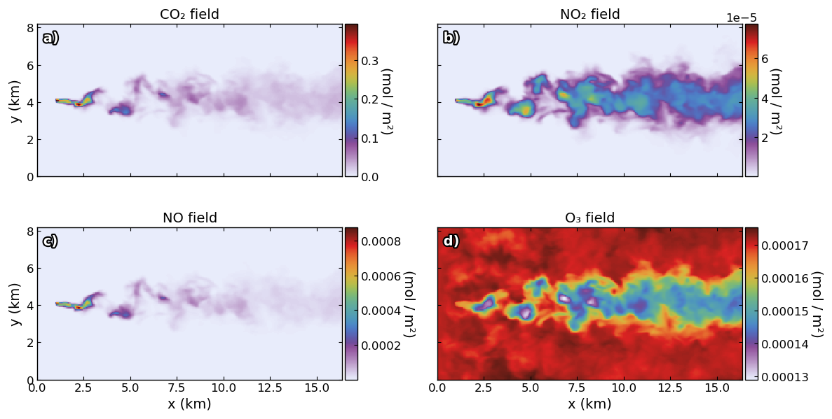
Figure 1 MicroHH large-eddy simulation of a coal-fired power plant plume at 64 m resolution for the 9 kmol s⁻¹ (12.5 Mt yr⁻¹) CO₂ emission case. The source (located at $(x_{\mathrm{0}},y_{\mathrm{0}},z_{\mathrm{0}})=(\mathrm{1024},\mathrm{4096},\mathrm{200})$ m) emits 9.0 kmol s⁻¹ (12.5 Mt yr⁻¹) CO₂, 0.0203 kmol s⁻¹ NO, and 0.00107 kmol s⁻¹ NO₂ into a 5 m s⁻¹ west-to-east wind field with 30 ppb background O₃. Column densities show: (a) CO₂ with maximum enhancement at the source, (b) NO₂ with maximum several kilometers downwind due to photochemical conversion from NO, (c) NO peaking at the source, and (d) O₃ depletion along the plume from NO titration. The spatial offset between CO₂ and NO₂ maxima demonstrates the coupled turbulent-chemical processes captured by the simulation.

3.2 Synthetic TANGO observations

Figure 1 shows a representative snapshot from the LES for the 12.5 Mt yr⁻¹ emission case. Panel (a) displays CO₂ column density, peaking at the source location with characteristic turbulent plume structure. Panel (c) shows NO column density, also maximizing at the source. Panel (b) shows NO₂ column density, with maximum enhancement several kilometers downwind due to chemical conversion from NO to NO₂ during advection. Panel (d) indicates O₃ depletion along the plume from NO titration reactions. The spatial offset between CO₂ and NO₂ enhancement maxima demonstrates the coupled turbulent-chemical processes that TANGO will observe.

To emulate TANGO measurements, MicroHH fields are processed through an observation operator that includes (1) vertical integration to obtain column densities, (2) convolution with a 2D Gaussian point spread function (300 m FWHM) to simulate instrument spatial response, and (3) data sampling on 300 m×300 m pixels. CO₂ and NO₂ can be sampled on spatially offset grids or from different temporal snapshots, simulating asynchronous observations expected from the two-satellite configuration. Finally, Gaussian measurement noise is added based on TANGO mission requirements: 0.576 mol m⁻² for CO₂ (approximately 1 % of the 420 ppm atmospheric background column) and $\mathrm{3.75}\times {\mathrm{10}}^{-\mathrm{5}}$ mol m⁻² for NO₂. Considering the maximum plume enhancements with respect to the atmospheric background, the NO₂ measurements exhibit approximately four times higher signal-to-noise ratio compared to CO₂. Figure 2a, b displays an example plume for the 12.5 Mt yr⁻¹ case after down-sampling to 300 m resolution and adding TANGO-representative measurement noise. These synthetic observations serve as the basis for Monte Carlo experiments as well as linear error propagation analyses to evaluate emission estimation performance and quantify uncertainties under various operational scenarios.

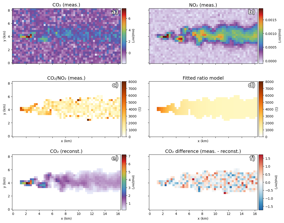
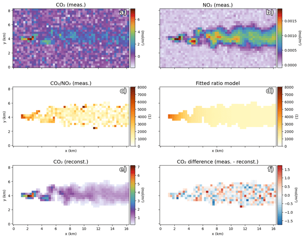
Figure 2 Demonstration of the CO₂–NO₂ plume reconstruction method using synthetic TANGO observations for the 12.5 Mt yr⁻¹ CO₂ emission case. The MicroHH plume from Fig. 1 is downsampled to 300 m resolution and Gaussian noise is added (CO₂: 0.576, NO₂: 3.75 × 10⁻⁵ mol m⁻²). Panels show: (a) noisy CO₂ observations, (b) less noisy NO₂ observations, (c) measured CO₂ $/$ NO₂ ratio exhibiting high variability, (d) smoothed ratio from exponential model fit (Eq. 4), (e) reconstructed CO₂ field with reduced noise obtained by scaling the measured NO₂ with the fitted ratio, and (f) difference between original and reconstructed CO₂ fields, dominated by measurement noise.

4 Methodology

To investigate the CO₂–NO₂ synergy of the TANGO observation concept, we exploit co-located CO₂ and NO₂ satellite observations to improve emission quantification and characterize atmospheric chemistry. The method leverages the typically higher signal-to-noise ratio of NO₂ plumes compared to CO₂ plumes at fine spatial resolution by empirically modeling the downwind evolution of the CO₂ $/$ NO₂ ratio. This section describes the ratio-based reconstruction approach and a simpler NO₂-based plume masking method, the IME for emission estimation, and the rigorous error propagation framework accounting for spatial correlations. Performance evaluation is presented in Sect. 5. Throughout this section, CO₂ and NO₂ denote retrieved column densities (mol m⁻²) after background subtraction. We note that in our simulation study the true background is known exactly from the LES, so background subtraction errors do not contribute to our uncertainty estimates; for real data errors in the background definition propagate directly into the integrated emission estimate. The approaches require CO₂ and NO₂ observations on a common spatial grid. When original retrievals are provided on different grids – as will be the case for TANGO's two formation-flying satellites – the NO₂ field is interpolated onto the CO₂ grid using smooth cubic spline interpolation. Figure 2a, b shows the CO₂ and NO₂ measurements for the 12.5 Mt yr⁻¹ case with typical measurement noise, as described in Sect. 3.2.

4.1 CO₂ $/$ NO₂ ratio model

To account for atmospheric conversion of NO to NO₂ and dilution downwind of an industrial source, the CO₂ $/$ NO₂ ratio is modeled by an exponential function (Meier et al., 2024):

$$\begin{array}{}\text{(1)}& F(s;\mathbf{x})=m_{\mathrm{1}}\exp \left(-{\displaystyle \frac{s}{{\mathit{\tau }}_{\mathrm{d}}}}\right)+m_{\mathrm{0}},\end{array}$$

here, s denotes the downwind Euclidean distance from the emission source, τ_d is the characteristic spatial decay length scale, m₁ is the initial amplitude of the ratio, and m₀ represents the asymptotic background value. The exponential parameterization represents the dominant physical processes: elevated CO₂ $/$ NO₂ ratios in the vicinity of the source (arising from direct CO₂ emissions and the initially limited formation of NO₂), followed by an exponential decrease as NO is oxidized to NO₂ and both species are subject to turbulent dilution. The three parameters τ_d, m₀, and m₁ that are summarized in a state vector

$$\begin{array}{}\text{(2)}& \mathbf{x}=({\mathit{\tau }}_{\mathrm{d}},m_{\mathrm{0}},m_{\mathrm{1}}{)}^T,\end{array}$$

provide quantitative, observation-based characterization of plume chemical evolution. The spatial decay parameter τ_d yields an effective chemical timescale when divided by the wind speed, the apparent source ratio m₁+m₀ characterizes the CO₂ $/$ NO₂ ratio at the emission location, and m₀ represents the background CO₂ $/$ NO₂ ratio downwind. Physical interpretation of these parameters is discussed in Sect. 5.

The functional form of Eq. (1) is physically motivated as follows. Freshly emitted NO_x is dominated by NO, so the NO₂ concentration is initially suppressed relative to its photostationary-state value. As NO is oxidized to NO₂, the CO₂ $/$ NO₂ ratio decreases from an initially elevated value toward a near-field asymptote m₀. The exponential term in Eq. (1) describes this approach to photostationary-state partitioning, while CO₂ acts as a conserved tracer on these scales. We emphasize that this is an empirical near-field approximation whose validity rests on the assumption that NO_x loss through secondary chemistry – primarily NO₂ + OH → HNO₃ – remains negligible within the analysis range. Any residual NO_x loss is implicitly absorbed into the fitted value of m₀, which should therefore be interpreted as an observational near-field diagnostic rather than a true physical ratio. This assumption is supported by the MicroHH simulation used in this study, which explicitly accounts for secondary chemistry losses. As shown in Fig. 2c, the modeled CO₂ $/$ NO₂ ratio remains constant across the far field within the simulation domain, confirming that NO_x loss through secondary chemistry is negligible on the scales considered here. This is consistent with Fig. 8 of Krol et al. (2024) and validates the assumption within the mission requirements. We note that Meier et al. (2024) applied the same functional form to the NO₂ $/$ NO_x ratio, where the ratio rises from near zero at the source to a photostationary-state plateau. The advantage of the CO₂ $/$ NO₂ ratio is that the relevant chemistry parameters can be determined by a fit, whereas they must be fitted or calibrated from additional information when working with the NO₂ $/$ NO_x ratio.

4.2 Ratio model fitting

To fit the model in Eq. (1) to observations, we first define the unitless ratio

$$\begin{array}{}\text{(3)}& y_i={\displaystyle \frac{[{\mathrm{CO}}_{\mathrm{2}}{]}_i}{[{\mathrm{NO}}_{\mathrm{2}}{]}_i}},\end{array}$$

as observable where [CO₂]_i and [NO₂]_i are the total column densities of the corresponding trace gases at spatial sampling point i. Assuming uncorrelated Gaussian measurement errors in CO₂ and NO₂ with standard deviations ${\mathit{\sigma }}_{i,{\mathrm{CO}}_{\mathrm{2}}}$ and ${\mathit{\sigma }}_{i,{\mathrm{NO}}_{\mathrm{2}}}$, the precision in y_i is obtained via standard error propagation:

$$\begin{array}{}\text{(4)}& {\displaystyle \frac{{\mathit{\sigma }}_{y_i}^{\mathrm{2}}}{y_i^{\mathrm{2}}}}={\displaystyle \frac{{\mathit{\sigma }}_{i,{\mathrm{CO}}_{\mathrm{2}}}^{\mathrm{2}}}{[{\mathrm{CO}}_{\mathrm{2}}{]}_i^{\mathrm{2}}}}+{\displaystyle \frac{{\mathit{\sigma }}_{i,{\mathrm{NO}}_{\mathrm{2}}}^{\mathrm{2}}}{[{\mathrm{NO}}_{\mathrm{2}}{]}_i^{\mathrm{2}}}}.\end{array}$$

For the measurement vector $\mathbf{y}=(y_{\mathrm{1}},\mathrm{\cdots },y_N)$, the corresponding error covariance matrix is given by

$$\begin{array}{}\text{(5)}& {\mathbf{S}}_y=\mathrm{diag}({\mathit{\sigma }}_{y_{\mathrm{1}}}^{\mathrm{2}},\mathrm{\dots },{\mathit{\sigma }}_{y_N}^{\mathrm{2}}).\end{array}$$

In the following, we assume that the measured ratio y can be represented by our model F(s_i;x), evaluated at the distance s_i between the sampling point i of the observation and the source location. This implicitly neglects a potential model bias arising from the fact that F describes the ratio of the underlying physical CO₂ and NO₂ fields, whereas the measurement y is a ratio of observed quantities whose numerator and denominator each correspond to a convolution of the true physical fields with the instrument's spatial response function. The higher the spatial resolution of the sensor, the smaller this bias is expected to be. In the following, we assume that for the TANGO spatial resolution of 300 m this error can be neglected; however, we will revisit this assumption when discussing systematic biases in the retrieved components of the state vector. Under this assumption, the state vector in Eq. (2) is estimated by minimizing the weighted least-squares cost function (Hansen, 2010):

$$\begin{array}{}\text{(6)}& {\mathbf{x}}_{\mathrm{ret}}=\arg {\min }_{\mathbf{x}}\left\{(\mathbf{y}-\mathbf{F}(\mathbf{x}\left){)}^{\mathrm{T}}{\mathbf{S}}_y^{-\mathrm{1}}\right(\mathbf{y}-\mathbf{F}\left(\mathbf{x}\right))\right\},\end{array}$$

where F(x) is the forward model vector with elements F(s_i;x) for each pixel. The minimization is performed using a Gauss–Newton iterative scheme, where a linearized least squares problem is solved per iteration step. After convergence, the solution is

$$\begin{array}{}\text{(7)}& {\mathbf{x}}_{\mathrm{ret}}=\mathbf{Gy}\end{array}$$

with the gain matrix

$$\begin{array}{}\text{(8)}& \mathbf{G}=({\mathbf{J}}^{\mathrm{T}}{\mathbf{S}}_y^{-\mathrm{1}}\mathbf{J}{)}^{-\mathrm{1}}{\mathbf{J}}^{\mathrm{T}}{\mathbf{S}}_y^{-\mathrm{1}}\end{array}$$

and the parameter covariance matrix

$$\begin{array}{}\text{(9)}& {\mathbf{S}}_x=({\mathbf{J}}^{\mathrm{T}}{\mathbf{S}}_y^{-\mathrm{1}}\mathbf{J}{)}^{-\mathrm{1}}.\end{array}$$

The forward model Jacobian J with

$$\begin{array}{}\text{(10)}& J_{i,k}={\displaystyle \frac{\partial F(s_i;\mathbf{x})}{\partial x_k}}\end{array}$$

is calculated at the expansion point of the last iteration step.

To ensure robust fitting, we filter out pixels in the measurement vector y with insufficient signal-to-noise: specifically, pixels where

$$\begin{array}{}\text{(11)}& {\displaystyle \frac{[{\mathrm{NO}}_{\mathrm{2}}{]}_i}{{\mathit{\sigma }}_{i,{\mathrm{NO}}_{\mathrm{2}}}}}<\mathrm{2}\text{or}{\displaystyle \frac{[{\mathrm{CO}}_{\mathrm{2}}{]}_i}{{\mathit{\sigma }}_{i,{\mathrm{CO}}_{\mathrm{2}}}}}<\mathrm{2}\end{array}$$

or where the unit-less ratio uncertainty ${\mathit{\sigma }}_{y_i}$ exceeds a predefined threshold. In this study we choose a threshold of 50 % of the ratio value. Only pixels passing these criteria are included in the measurement vector. This signal-to-noise selection criterion is functionally equivalent to a plume mask applied jointly to the CO₂ and NO₂ fields, as is also evident from Fig. 2c, d. Note that the same NO₂-derived mask used in the masking approach can optionally be applied to the reconstruction approach here as well. Figure 2d shows the modeled CO₂ $/$ NO₂ ratio using Eq. (1) for the 12.5 Mt yr⁻¹ base case, illustrating how the model captures the essential chemistry and transport processes represented in the MicroHH simulation shown in Fig. 2c. The model is applied directly to the CO₂ $/$ NO₂ ratio, so finite spatial resolution mainly affects the source ratio m₁+m₀, while the decay scale τ_d and m₀ characterization is discussed in Sect. 5.

4.3 CO₂ plume reconstruction

After the model fit, a CO₂ field can be derived from the NO₂ measurements by

$$\begin{array}{}\text{(12)}& [{\mathrm{CO}}_{\mathrm{2}}{]}_i^{\mathrm{recon}}=F(s_i;{\mathbf{x}}_{\mathrm{ret}})\cdot [{\mathrm{NO}}_{\mathrm{2}}{]}_i.\end{array}$$

The error covariance matrix S_recon of the reconstructed [CO₂]^recon field is given by

$$\begin{array}{}\text{(13)}& \begin{array}{rl}{\mathbf{S}}_{\mathrm{recon},ij}& =\left[{\mathrm{NO}}_{\mathrm{2}}{]}_i\right[{\mathrm{NO}}_{\mathrm{2}}{]}_j{\mathbf{J}}_i{\mathbf{S}}_x{\mathbf{J}}_j^{\mathrm{T}}\\ & +{\mathit{\delta }}_{ij}{F}^{\mathrm{2}}(s_i;{\mathbf{x}}_{\mathrm{ret}}){\mathit{\sigma }}_{i,{\mathrm{NO}}_{\mathrm{2}}}^{\mathrm{2}},i,j=\mathrm{1},\mathrm{\dots },N,\end{array}\end{array}$$

where J_i denotes the ith row of the Jacobian matrix J, S_x is the covariance matrix of the fitted model parameters, ${\mathit{\sigma }}_{{\mathrm{NO}}_{\mathrm{2}}}$ is the NO₂ measurement noise standard deviation, and δ_ij is the Kronecker delta. The second term on the right-hand side of the equation describes uncorrelated CO₂ errors due to a scaling of corresponding NO₂ errors, whereas the first term describes correlated CO₂ errors due to the errors on the model parameter x.

Figure 2e shows the reconstructed CO₂ field for the 12.5 Mt yr⁻¹ case, which exhibits reduced noise compared to the original CO₂ measurement. The difference between the reconstructed and original CO₂ fields (Fig. 2f) primarily reflects the filtered measurement noise in the first term in Eq. (13). The implications of this noise reduction for integrated emission uncertainty are evaluated in Sect. 5. By design, the ratio model can represent only those spatial and temporal structures that are describable by the three fitted parameters. Consequently, systematic errors that are present in the CO₂ column density product but absent in the corresponding NO₂ field are substantially mitigated by the fitting procedure. For example, retrieval artifacts – such as striping or surface-related structures – that affect CO₂ and NO₂ differently are partially suppressed.

4.4 Sensitivity analysis

To assess the effective information content of the reconstruction, we compute the sensitivity of ${\mathrm{CO}}_{\mathrm{2}}^{\mathrm{recon}}$ to the true CO₂ signal using a pixel-wise sensitivity matrix, analogous to an averaging kernel (Rodgers, 2000):

$$\begin{array}{}\text{(14)}& A_{ij}={\displaystyle \frac{\partial [{\mathrm{CO}}_{\mathrm{2}}{]}_i^{\mathrm{recon}}}{\partial [{\mathrm{CO}}_{\mathrm{2}}{]}_j^{\mathrm{true}}}}={\displaystyle \frac{[{\mathrm{NO}}_{\mathrm{2}}{]}_i}{[{\mathrm{NO}}_{\mathrm{2}}{]}_j}}\cdot {\left(\mathbf{J}\cdot \mathbf{G}\right)}_{ij}.\end{array}$$

Matrix A quantifies how strongly [CO₂]^recon responds to the true [CO₂]^true signal:

$$\begin{array}{}\text{(15)}& [{\mathrm{CO}}_{\mathrm{2}}{]}^{\mathrm{recon}}=\mathbf{A}\cdot [{\mathrm{CO}}_{\mathrm{2}}{]}^{\mathrm{true}}.\end{array}$$

The complementary term 1−A_ii defines the fraction of the signal not captured by the model, representing the null-space error of the reconstruction approach (Borsdorff et al., 2014). This sensitivity analysis quantifies the extent to which the reconstructed CO₂ field faithfully represents the true atmospheric state versus being influenced by the NO₂ observations and model constraints.

Figure 3 illustrates the application of the averaging kernel A for the 12.5 Mt yr⁻¹ base case. To stress-test the method, we define the true CO₂ field as a plume from 9 min before the time step used to derive A (Fig. 3a); this represents an extreme case, as the temporal separation between CO₂ and NO₂ observations from TANGO will be less than 1 min in practice. When A is applied to this earlier plume according to Eq. (15), the reconstructed field (Fig. 3b) exhibits turbulence patterns from the later NO₂ plume used to construct A, demonstrating that reconstruction always responds with the turbulence features of the NO₂ field rather than the true CO₂ field. The difference field (Fig. 3c) reveals this temporal mismatch in turbulent structures. This represents a fundamental limitation of the method: reconstruction performance depends critically on temporal alignment between CO₂ and NO₂ observations, degrading when CO₂ and NO₂ plume structures begin to de-correlate. Although the 9 min separation used here is far larger than what TANGO will experience, it serves to clearly expose this sensitivity. Quantitative evaluation of temporal separation effects, including sub-minute separations representative of TANGO, is presented in Sect. 5.

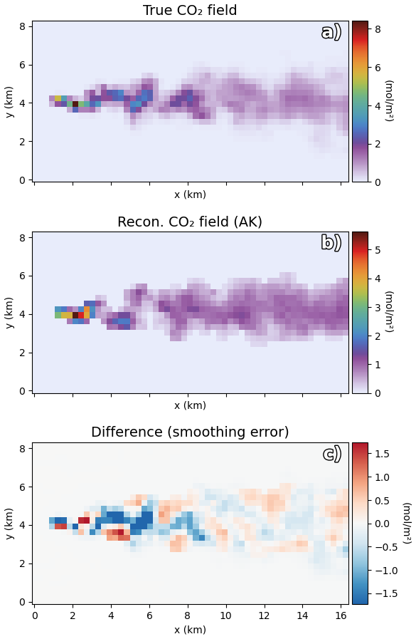
Figure 3 Application of the averaging kernel A for the 12.5 Mt yr⁻¹ emission case demonstrating sensitivity to temporal alignment between CO₂ and NO₂ observations. (a) True CO₂ field from a plume 9 min before the time step used to calculate A. (b) Reconstructed CO₂ field when A (derived from the last ensemble plume) is applied to the earlier plume from panel (a) according to Eq. (15), showing turbulence patterns from the later NO₂ plume that are inconsistent with the true field in panel (a). (c) Difference between panels (b) and (a), revealing the turbulence mismatch. This demonstrates that reconstruction always responds with the turbulence features of the NO₂ field used to construct A, representing a fundamental limitation that requires temporal co-location between CO₂ and NO₂ observations.

4.5 NO₂-based plume masking

As a simpler alternative to full reconstruction, NO₂ observations can be used to define a plume mask that identifies the spatial extent of the emission plume. A threshold is applied to the NO₂ field to identify pixels within the plume, and the CO₂ emission is then estimated by integrating only those CO₂ pixels that fall within this mask. This approach avoids the complexity of ratio fitting while still leveraging NO₂'s superior signal-to-noise ratio for plume detection.

The masking threshold is chosen to balance two competing effects: setting the threshold too low includes background noise and increases random error, while setting it too high truncates the true plume extent and introduces systematic bias. An optimal threshold can be determined empirically by minimizing the total error (combining bias and random uncertainty). Performance evaluation and threshold optimization are presented in Sect. 5.

This NO₂-based masking approach is conceptually related to the neighboring-pixel background estimation methods of Kuhlmann et al. (2019) and Varon et al. (2018), both of which use spatial information from adjacent pixels to define the plume boundary and background level. The use of NO₂ for plume detection has been explored in previous multi-species emission studies (Kuhlmann et al., 2019; Reuter et al., 2019). Here, our threshold is applied to the co-emitted NO₂ field rather than to the target species CO₂ itself, exploiting NO₂'s superior signal-to-noise ratio for spatially coherent plume delineation independent of CO₂ noise.

4.6 Emission estimation using the IME method

To estimate the total emission rate E, we employ the IME method. Fundamentally, the emission rate equals the total plume mass divided by the plume residence time: $E=M/t_{\mathrm{trans}}$, where $t_{\mathrm{trans}}=L/U$ is the plume transit time, L is the plume length along the wind direction, and U is the effective mass-weighted wind speed. Discretizing to pixels yields (Santaren et al., 2025; Kuhlmann et al., 2024):

$$\begin{array}{}\text{(16)}& E={\displaystyle \frac{\mathrm{\Delta }a}{t_{\mathrm{trans}}}}\sum _{i\in I}[{\mathrm{CO}}_{\mathrm{2}}{]}_i,\end{array}$$

where I denotes pixels within the plume boundary and Δa is the pixel area (assumed constant). We note that this distance-based formulation differs from the Varon et al. (2018) implementation, which uses $L=\sqrt{A}$ and large-eddy simulation calibration of the effective wind speed (Kuhlmann et al., 2024).

For the reconstruction approach, [CO₂]_i is replaced by the reconstructed field $[{\mathrm{CO}}_{\mathrm{2}}{]}_i^{\mathrm{recon}}$ from Eq. (12); pixel selection is performed through the signal-to-noise filter in Eq. (11), which is functionally equivalent to a plume mask. For the masking approach, the original CO₂ observations are used, with the summation restricted to pixels identified by the NO₂-derived mask.

The precision σ_E of the flux estimate E is derived from the error covariance of the CO₂ field by

$$\begin{array}{}\text{(17)}& {\mathit{\sigma }}_E^{\mathrm{2}}={\mathbf{K}}_{{\mathrm{CO}}_{\mathrm{2}}}^{\mathrm{T}}{\mathbf{S}}_{{\mathrm{CO}}_{\mathrm{2}}}{\mathbf{K}}_{{\mathrm{CO}}_{\mathrm{2}}},\end{array}$$

where ${\mathbf{K}}_{i,{\mathrm{CO}}_{\mathrm{2}}}=\partial E/\partial [{\mathrm{CO}}_{\mathrm{2}}{]}_i=\mathrm{\Delta }a/t_{\mathrm{trans}}$ is the derivative linking each pixel's CO₂ value to the total emission, and ${\mathbf{S}}_{{\mathrm{CO}}_{\mathrm{2}}}$ is the covariance of the CO₂ field. For reconstruction, ${\mathbf{S}}_{{\mathrm{CO}}_{\mathrm{2}}}={\mathbf{S}}_{\mathrm{recon}}$ from the previous subsection, which includes spatial correlations introduced by the ratio fitting. For masking, ${\mathbf{S}}_{{\mathrm{CO}}_{\mathrm{2}}}$ represents the diagonal measurement error covariance of the original CO₂ observations.

Critical to proper uncertainty quantification is rigorous error propagation accounting for the full error covariance matrix, including off-diagonal spatial correlations. For reconstruction-based methods, these correlations arise from the ratio fitting process and can dominate the integrated emission uncertainty even when pixel-level noise appears reduced. The impact of these correlations on emission uncertainty is quantified in Sect. 5.

5 Results

We assess the performance of CO₂ emission estimation and chemistry parameter retrieval using the synthetic TANGO observations for four emission scenarios: 2.0, 2.5, 5.0, and 12.5 Mt yr⁻¹, as outlined in Sect. 3.2. This allows direct comparison between analytical precision calculations and Monte Carlo simulations under realistic TANGO-like noise conditions. Monte Carlo simulations were performed using 10 independent MicroHH plume realizations, with 500 Gaussian noise realizations added to both CO₂ and NO₂, and emission rates computed via the IME method. This setup enables evaluation of both the CO₂ $/$ NO₂ ratio reconstruction and simpler NO₂-based plume masking approaches in terms of precision, bias, and noise propagation. In addition, the methods are applied to EnMAP satellite observations to demonstrate feasibility and robustness on real-world data.

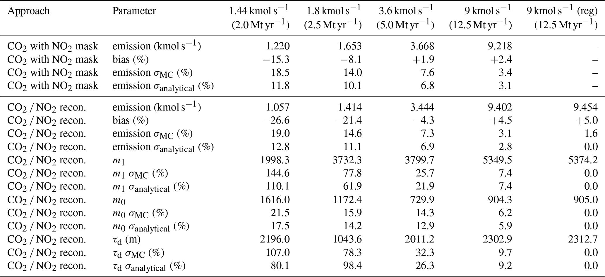
Table 1 Comparison of emission estimates and model parameters for different CO₂ emission strengths using two approaches: (i) emission estimation from CO₂ observations using an NO₂-derived plume mask, and (ii) joint CO₂–NO₂ reconstruction. Results are shown for four emission strengths: 1.44 (2.0 Mt yr⁻¹), 1.8 (2.5 Mt yr⁻¹), 3.6 (5.0 Mt yr⁻¹), and 9 kmol s⁻¹ (12.5 Mt yr⁻¹). Retrieved values are shown with relative precision estimates reported as percentages: σ_MC denotes Monte Carlo standard deviation and σ_analytical denotes the analytical error estimate. Emission bias is reported relative to the true emission. In all cases, perfect co-location in time and space between CO₂ and NO₂ observations is assumed. The last column (9 kmol s⁻¹ reg) shows the joint CO₂–NO₂ reconstruction with chemical parameters fixed to values derived from noise-free simulations, illustrating the impact of parameter regularization on error characteristics.

5.1 Emission estimation performance

Table 1 presents comprehensive emission estimation results for both NO₂-based masking and CO₂ $/$ NO₂ reconstruction approaches across all four emission strengths under ideal conditions – perfect spatial and temporal co-location. Performance depends strongly on source strength, revealing a clear hierarchy in method applicability.

At the lowest emission strength of 2.0 Mt yr⁻¹, both approaches show substantial limitations. The NO₂ masking approach retrieves 1.22 kmol s⁻¹ with a bias of −15.3 % and precision of 18.5 % (Monte Carlo) or 11.8 % (analytical). The reconstruction approach performs worse, retrieving 1.06 kmol s⁻¹ with a bias of −26.6 % and precision of 19.0 % (Monte Carlo) or 12.8 % (analytical). These substantial biases reflect persistent ratio fitting errors when the CO₂ signal is weak relative to measurement noise. The insufficient CO₂ signal-to-noise ratio prevents reliable characterization of the ratio evolution, leading to systematic underestimation of the true emission in a non-linear least squares fit. Chemistry parameters at this emission level exhibit uncertainties exceeding 100 % for m₁ and τ_d, rendering them uninterpretable. This emission strength falls below TANGO's operational detection threshold. At 2.5 Mt yr⁻¹, representing TANGO's nominal detection limit, the NO₂ masking approach shows marked improvement: 1.65 kmol s⁻¹ retrieved emission with −8.1 % bias and 14.0 % precision (Monte Carlo) or 10.1 % (analytical). In contrast, the reconstruction approach still exhibits substantial bias: 1.41 kmol s⁻¹ with −21.4 % bias and 14.6 % precision (Monte Carlo) or 11.1 % (analytical). While both methods achieve similar precision (14 %–15 %), the masking approach demonstrates superior bias characteristics, making it operationally preferable for weak sources near the detection threshold. Chemistry parameters remain poorly constrained, with m₁ uncertainty at 77.8 % and τ_d uncertainty at 78.3 %, precluding meaningful atmospheric interpretation.

At an emission rate of 5.0 Mt yr⁻¹, both retrieval strategies achieve acceptable performance. The masking method yields an inferred flux of 3.67 kmol s⁻¹ with a bias of +1.9 % and a precision of 7.6 % (Monte Carlo estimate) or 6.8 % (analytical estimate). The reconstruction method yields 3.44 kmol s⁻¹ with a bias of −4.3 % and a precision of 7.3 % (Monte Carlo) or 6.9 % (analytical). For both approaches, the precision is on the order of 7 %, and the biases are reduced to within ± 5 %. This emission level thus marks a critical threshold at which the CO₂ signal becomes sufficiently strong to enable robust characterization of concentration ratios. At this emission magnitude, the inferred chemistry parameters become physically interpretable: m₁=3799.7 with a relative precision of 25.7 %, m₀=729.9 with 14.3 % precision, and τ_d=2011.2 m with 32.3 % precision. Although the associated uncertainties remain considerable, they are sufficiently constrained to allow qualitative evaluation of the plume chemistry evolution. At the highest emission strength of our study of 12.5 Mt yr⁻¹, both methods achieve robust performance. The masking approach retrieves 9.22 kmol s⁻¹ with +2.4 % bias and 3.4 % precision (Monte Carlo) or 3.1 % (analytical). The reconstruction approach retrieves 9.40 kmol s⁻¹ with +4.5 % bias and 3.1 % precision (Monte Carlo) or 2.8 % (analytical). Both approaches achieve approximately 3 % emission precision with small biases below 5 %, demonstrating the fundamental method capabilities under optimal signal conditions. Chemistry parameters are well-constrained: m₁=5349.5 with 7.4 % uncertainty, m₀=904.3 with 6.2 % uncertainty, and τ_d=2302.9 m with 9.7 % uncertainty, enabling quantitative characterization of atmospheric chemistry processes. Across all emission strengths, Monte Carlo and analytical uncertainties agree within 1–2 percentage points, validating the linear error propagation framework described in Sect. 4. The final column of Table 1 shows that fixing chemistry parameters to true values (known from noise-free simulations) reduces emission uncertainty by approximately a factor of two for the 12.5 Mt yr⁻¹ case (1.6 % versus 3.1 %), demonstrating best-case performance with perfect prior knowledge – unavailable operationally.

5.2 Method comparison: masking versus reconstruction

Direct comparison between NO₂-based masking and CO₂ $/$ NO₂ reconstruction reveals a counter-intuitive central finding: despite producing visually cleaner CO₂ fields with suppressed pixel-scale noise (Fig. 2), reconstruction does not improve emission precision relative to simple masking. At low emissions (2.0 and 2.5 Mt yr⁻¹), masking shows superior bias characteristics (−15.3 % and −8.1 %) compared to reconstruction (−26.6 % and −21.4 %). At intermediate and high emissions (5.0 and 12.5 Mt yr⁻¹), both achieve comparable accuracy with biases within ± 2 %–5 %. Precision remains essentially equivalent across all emission strengths: approximately 19 %, 14 %, 7 %, and 3 % for the four cases, respectively. For emission estimates, this precision equivalence despite markedly different noise appearance of the plume requires careful explanation. The reconstruction process fits a three-parameter exponential function to the observed CO₂ $/$ NO₂ ratio, which cannot capture high-frequency pixel-scale fluctuations. The uncorrelated CO₂ measurement noise enters the ratio and maps onto the fitted parameters (m₀, m₁, τ_d). When the fitted ratio is multiplied by NO₂ to reconstruct CO₂ (Eq. 12), pixel-scale noise variability is suppressed (first term in Eq. 13), but spatial correlations of noise spanning the entire plume extent are introduced. The uncorrelated errors due to direct mapping of the NO₂ error (second term in Eq. 13) is not a dominant error term.

For spatial integration in the IME method, the error correlations dominate total uncertainty because the individual errors on the CO₂ columns coherently add rather than cancel. In contrast, uncorrelated pixel noise in the original CO₂ field (used by the masking approach) averages out during integration, following ${\mathit{\sigma }}_{\mathrm{total}}\propto \sqrt{N}$ scaling. This behavior applies generically to any method using NO₂ to smooth, regularize, or reconstruct CO₂ fields. A critical implication of this is that such methods must provide complete error covariance matrices to demonstrate genuine error reduction. Computing emission precision neglecting spatial correlations introduced by the fitting or smoothing process, can severely underestimate the precision of the emission estimates. In our reconstruction approach, accounting for the full covariance matrix (off-diagonal terms in S_recon) increases the integrated emission uncertainty by more than a factor of 60 compared to cases ignoring error correlation.

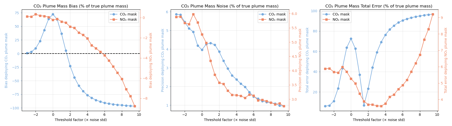
Figure 4 Trade-off between bias and noise in CO₂ plume mass estimation as a function of detection threshold for the 9 kmol s⁻¹ (12.5 Mt yr⁻¹) CO₂ emission case. Two masking strategies are compared: applying a threshold to CO₂ observations (blue) versus NO₂ observations (red), with thresholds defined as multiples of the respective noise standard deviations (${\mathit{\sigma }}_{{\text{CO}}_{\mathrm{2}}}$ = 0.576 mol m⁻², ${\mathit{\sigma }}_{{\text{NO}}_{\mathrm{2}}}=\mathrm{3.75}\times {\mathrm{10}}^{-\mathrm{5}}$ mol m⁻²). Note that the x-axis unit differs between the two curves: a threshold factor of 1 corresponds to 0.576 mol m⁻² for CO₂ (blue) and $\mathrm{3.75}\times {\mathrm{10}}^{-\mathrm{5}}$ mol m⁻² for NO₂ (red). Panels show results from Monte Carlo analysis (N=1000): (a) systematic bias in retrieved CO₂ plume mass, (b) random error (standard deviation) in mass estimates, and (c) total error ($\sqrt{{\text{bias}}^{\mathrm{2}}+{\mathit{\sigma }}^{\mathrm{2}}}$). All errors are expressed as percentage of true plume mass.

Coming back to the plume masking approach, Fig. 4 quantifies the trade-off between emission bias and precision for different masking thresholds for the 12.5 Mt yr⁻¹ case. Two masking strategies are compared: applying a threshold to CO₂ observations (blue) versus NO₂ observations (red), with thresholds defined as multiples of the respective noise standard deviations (${\mathit{\sigma }}_{{\text{CO}}_{\mathrm{2}}}=\mathrm{0.576}$, ${\mathit{\sigma }}_{{\text{NO}}_{\mathrm{2}}}=\mathrm{3.75}\times {\mathrm{10}}^{-\mathrm{5}}$ mol m⁻²). Without masking (threshold <0), plume mass is unbiased but exhibits the largest random error as the entire background noise is integrated (Fig. 4b). Thresholding CO₂ reduces precision but rapidly increases bias: low thresholds preferentially exclude negative noise creating positive bias (Fig. 4a), while high thresholds truncate true signal causing negative bias. Figure 4c shows total error defined by $e_{\mathrm{tot}}=\sqrt{{\text{b}}^{\mathrm{2}}+{\mathit{\sigma }}^{\mathrm{2}}}$ with precision σ and bias b. It demonstrates that no single CO₂ threshold achieves robust performance across the full bias-precision trade-off.

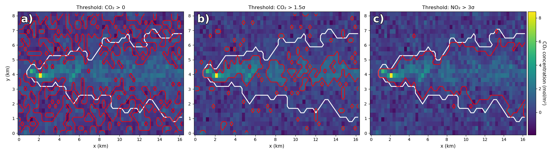
Figure 5 Illustration of plume masking for different detection thresholds for the 12.5 Mt yr⁻¹ CO₂ emission case, corresponding to selected points in Fig. 4. Background colors show the CO₂ column enhancement field. The true plume mask is shown in white, while the estimated plume mask is shown in red. Panels (a) and (b) apply threshold filtering directly to CO₂ observations using the CO₂ noise standard deviation. Panel (c) applies threshold filtering to NO₂ observations, which is subsequently used as a plume mask for CO₂. The examples highlight how CO₂-based masking is increasingly affected by noise at low thresholds and by plume truncation at high thresholds, whereas NO₂-based masking provides a more spatially coherent plume delineation for comparable noise levels.

Figure 5 illustrates spatial effects of a NO₂ masking strategies for the CO₂ plume mask. The true plume mask (white contour, 0.008 mol m⁻² threshold from noise-free CO₂) serves as reference. Panel (a) with CO₂>0 shows isolated noise features inflating integrated mass. Panel (b) with CO${}_{\mathrm{2}}>\mathrm{1.5}{\mathit{\sigma }}_{{\text{CO}}_{\mathrm{2}}}$ suppresses noise but truncates plume edges. Panel (c) demonstrates NO₂-derived masking: a threshold of $\mathrm{3}{\mathit{\sigma }}_{{\text{NO}}_{\mathrm{2}}}$ yields <1 % bias and approximately 2 % random error, closely following the true plume extent while avoiding both noise contamination and premature truncation. This NO₂-based approach represents approximately a factor-of-two improvement in precision compared to analyzing CO₂ without NO₂ guidance. Thus for TANGO emission quantification, we recommend NO₂-based masking: it is computationally simpler than reconstruction, exhibits superior bias characteristics for weak sources below 5 Mt yr⁻¹, and achieves equivalent precision across all emission strengths. The main value of the reconstruction approach lies in enabling chemistry parameter retrieval, discussed in the following subsection.

5.3 Chemistry parameter retrieval

As outlined in Sect. 4.1, the fit of the model in Eq. (1) to CO₂ and NO₂ observations simultaneously retrieves three chemistry parameters: the spatial decay scale τ_d, the amplitude m₁, and the background ratio m₀, with the apparent source ratio given by m₁+m₀ (Table 1). These parameters describe plume evolution processes, complementing emission estimates. The quality of the retrieved parameters depends critically on emission strength, following the same hierarchy observed for emission quantification. At 2.0 and 2.5 Mt yr⁻¹, chemistry parameters are uninterpretable due to errors exceeding 70 %–100 %. Weak CO₂ signals provide insufficient information to constrain the ratio evolution. At 5.0 Mt yr⁻¹, parameters become interpretable: m₁=3799.7 (25.7 % precision), m₀=729.9 (14.3 % precision), and τ_d=2011.2 m (32.3 % precision). While uncertainties remain substantial, they permit qualitative assessment of plume chemistry. At 12.5 Mt yr⁻¹, robust retrieval is achieved: m₁=5349.5 (7.4 % precision), m₀=904.3 (6.2 % precision), and τ_d=2302.9 m (9.7 % precision), enabling quantitative characterization. Overall, the interpretation of these parameters even for moderate precisions requires careful consideration of observational constraints and potential biases.

The spatial decay parameter τ_d exhibits the clearest interpretation among the three fitted parameters. Retrieved values of 2100–2300 m for the medium and large emission cases substantially exceed TANGO's 300 m point spread function, indicating that τ_d represents a genuine atmospheric process which is little affected by the forward model error that we discussed in Sect. 4.2. The decay scale characterizes the spatial evolution of the CO₂ $/$ NO₂ ratio along the plume: higher values indicate slower ratio changes, while lower values indicate rapid decay. When combined with information on the wind speed U in the plume direction, τ_d converts to an effective chemical timescale ${\mathit{\tau }}_s={\mathit{\tau }}_{\mathrm{d}}/U$ that quantifies the effective rate of NO → NO₂ conversion relative to the conservative tracer CO₂.

In the simulation, the background O₃ concentration is 30 ppb and the rate coefficient for NO + O₃ → NO₂ + O₂ is $k=\mathrm{1.9}\times {\mathrm{10}}^{-\mathrm{14}}$ cm³ molec.⁻¹ s⁻¹, giving a theoretical clean-air NO lifetime of ${\mathit{\tau }}_{\mathrm{chem}}=\left(k\right[{\mathrm{O}}_{\mathrm{3}}]{)}^{-\mathrm{1}}\approx \mathrm{70}$ s. The competing photolysis reaction ${\mathrm{NO}}_{\mathrm{2}}+h\mathit{\nu }\to \mathrm{NO}+\mathrm{O}$ partly counteracts this conversion, with a daytime timescale of ∼300 s, so the net NO→NO₂ conversion in clean air is slower than the 70 s lower limit. In practice, however, the fresh plume rapidly titrates local O₃, reducing its concentration and substantially lengthening the effective conversion timescale. The degree of this ozone depletion is controlled by turbulent mixing: faster dilution replenishes background O₃ more quickly, shortening τ_s, while slower dilution sustains O₃ depletion and extends it. The retrieved τ_s therefore encodes both chemistry and plume dynamics. For the simulation, the imposed boundary wind is 5 m s⁻¹, but surface friction reduces the effective mass-weighted wind speed within the plume to approximately 4 m s⁻¹, yielding ${\mathit{\tau }}_s={\mathit{\tau }}_{\mathrm{d}}/U\approx \mathrm{2300}\mathrm{m}/\mathrm{4}\mathrm{m}{\mathrm{s}}^{-\mathrm{1}}\approx \mathrm{575}$ s.

The apparent source ratio m₁+m₀ nominally represents the CO₂ $/$ NO₂ ratio extrapolated back to the emission source location. This does not correspond to the true CO₂ $/$ NO_x emission ratio, since in the MicroHH setup 95 % of the emitted NO_x is assumed to be released as NO rather than NO₂. For the 12.5 Mt yr⁻¹ case, the retrieved value is $m_{\mathrm{1}}+m_{\mathrm{0}}=\mathrm{5349.5}+\mathrm{904.3}=\mathrm{6253.8}$. In principle, this could reveal information about combustion characteristics, fuel composition, or emission control technologies. However, this parameter is biased by more than 25 % at TANGO's 300 m spatial resolution, preventing direct interpretation as the true emission ratio without careful correction. This bias arises from the limited spatial resolution of satellite instruments, which cannot fully resolve the narrow plumes near the source. Where the ratio model describes the ratio of “real” fields, the observed ratio is affected by the instrument spatial response that blurs the observed CO₂ and NO₂ field independently. This affects the accuracy of the retrieved quantity m₁+m₀ which is mainly determined at the source location of the plume. Consequently, m₁+m₀ cannot be directly interpreted as the true CO₂ $/$ NO₂ emission ratio without accounting for these resolution-dependent biases.

Finally, we discuss the background ratio m₀, which represents the empirical CO₂ $/$ NO₂ ratio in the far downwind portion of the plume within the near-field validity range of the model – i.e., where the NO → NO₂ conversion is essentially complete but NO_x loss through secondary chemistry remains small. Retrieved m₀ values range from approximately 730 to 900 for the larger emission cases (Table 1). Given its definition, one might wish to use m₀ to infer the true background CO₂ $/$ NO_x emission ratio. However, any conversion of m₀ to this underlying emission ratio depends on atmospheric parameters that are not directly constrained by the TANGO observations, such as the degree of O₃ depletion within the plume. Despite this limitation in interpretability, m₀ remains valuable as an empirical diagnostic: it represents the CO₂ $/$ NO₂ ratio far downwind where the plume has diluted sufficiently for background air to dominate, restoring the ambient CO₂ $/$ NO₂ ratio. Systematic variations in m₀ across different locations or atmospheric regimes can therefore provide insight into differences in background composition and plume-chemistry evolution, even if its absolute value cannot be unambiguously related to intrinsic emission characteristics. Within the plume lengths analysed here (<15 km), NO_x oxidation via NO₂ + OH (lifetime ∼2 h) is a secondary effect; however, its influence is implicitly absorbed into the fitted parameters, in particular m₀, which encodes the far-field CO₂ $/$ NO₂ ratio where such processing has already modified the NO₂ $/$ NO_x partitioning.

5.4 Robustness to spatial and temporal misalignment

Up to this point, the CO₂–NO₂ synergy has been analyzed under the idealized assumption of perfectly aligned observations of both species. For TANGO, however, due to the configuration comprising the two CubeSats TANGO-Carbon and TANGO-Nitro, the CO₂ and NO₂ measurements are neither spatially nor temporally fully co-located. To assess the robustness of our methodology under realistic TANGO operational conditions, we again consider the 12.5 Mt yr⁻¹ base case and conduct an extensive Monte Carlo experiment: 10 independent MicroHH plume snapshots are each combined with 500 distinct noise realizations, resulting in 5000 total realizations per configuration. Both the masking and reconstruction strategies are then evaluated for their sensitivity to spatial and temporal misalignment between the CO₂ and NO₂ observations, simulated by sampling CO₂ and NO₂ on shifted grids and by selecting plume snapshots with varying time separations.

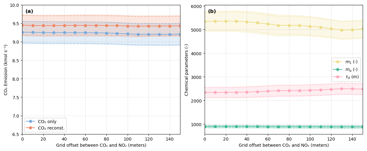
Figure 6 Robustness of emission estimates (a) and retrieved chemistry parameters m₁+m₀, m₀, and τ_d (b) to spatial grid misalignment between CO₂ and NO₂ observations for the 9 kmol s⁻¹ (12.5 Mt yr⁻¹) case. Monte Carlo results from 10 MicroHH plume snapshots, each combined with 500 noise realizations. Blue symbols: CO₂-only emission estimates (independent of grid shift); orange symbols: reconstructed CO₂ estimates. Error bars show Monte Carlo standard deviations; dotted lines denote analytical error estimates. Both emissions and chemistry parameters remain stable for grid offsets up to 150 m (half a TANGO pixel): emission biases stay below 2 % with ∼ 50 % lower uncertainties for the reconstruction, and chemistry parameters fluctuate by less than 5 %, well within their 7 %–10 % retrieval uncertainties.

5.4.1 Spatial grid misalignment

Figure 6 examines the effect of spatial misalignment between the CO₂ and NO₂ observation grids. The NO₂ grid is shifted systematically in both x and y directions by distances up to 150 m (half a TANGO pixel), and emission estimates are computed for both masking and reconstruction approaches. Blue symbols show emissions estimated from CO₂ only (independent of grid shift), orange symbols show emissions from reconstructed CO₂ using NO₂ measurements. Error bars indicate the standard deviation across noise realizations, while dotted lines denote analytically derived error estimates. Both methods show excellent stability: emission biases remain below 2 % for grid shifts up to 150 m. Monte Carlo and analytical uncertainties closely match across all tested offsets, confirming that the error propagation framework correctly accounts for spatial misalignment effects. Chemistry parameters retrieved via reconstruction are similarly robust: m₁+m₀, m₀, and τ_d fluctuate by less than 5 %, well within their 7 %–10 % retrieval uncertainties. Thus, spatial grid alignment is not a critical error source for TANGO, even for misalignments up to half a pixel.

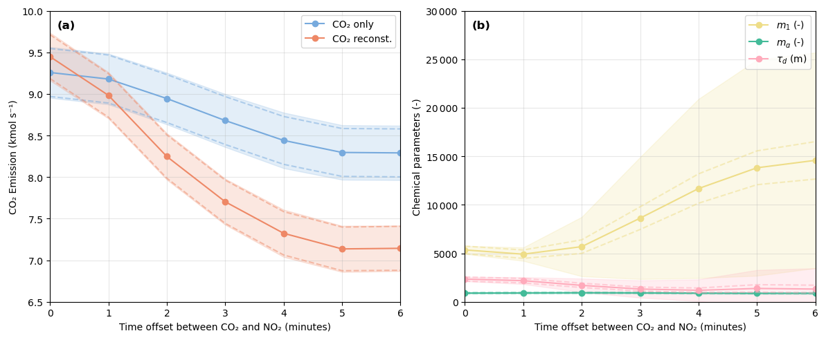
Figure 7 Robustness of emission estimates (a) and retrieved chemistry parameters m₁+m₀, m₀, and τ_d (b) to temporal separation between CO₂ and NO₂ measurements for the 9 kmol s⁻¹ (12.5 Mt yr⁻¹) case. Monte Carlo results from 10 MicroHH plume snapshots at 1 min intervals, each combined with 500 noise realizations. Blue symbols: CO₂-only emission estimates (independent of temporal offset); orange symbols: reconstructed CO₂ estimates. Error bars show Monte Carlo standard deviations; dotted lines denote analytical error estimates. At TANGO's nominal 60 s separation, emission biases are below 2 % and chemistry parameters vary by less than 3 % (m₁+m₀), 5 % (m₀), and 8 % (τ_d). Beyond 2 min, τ_d increases systematically as plume evolution introduces ratio fluctuations unrelated to chemistry, marking the practical upper limit for reliable parameter retrieval.

5.4.2 Temporal separation

Figure 7 quantifies the effect of temporal offset between CO₂ and NO₂ measurements. The MicroHH simulation provides plume snapshots at 1 min intervals, enabling evaluation of how time delays between the two satellite observations affect the data interpretation. CO₂ and NO₂ fields are sampled from different time steps to simulate temporal offsets from 0 to 9 min, with emissions and chemistry parameters computed for both approaches. At TANGO's nominal 60 s separation, both approaches exhibit emission biases below 2 %. The masking approach maintains this performance to approximately 2 min, with biases increasing gradually beyond this point. The reconstruction approach shows similar robustness up to 2–3 min (bias < 6 %), with substantial deviations only beyond 4 min (28 % bias at 6 min). These degradations at long temporal separations reflect turbulent transport breaking the simultaneity assumption: turbulent plume structures evolve on timescales of several minutes, and when CO₂ and NO₂ observations sample substantially different plume realizations, the ratio-based reconstruction introduces systematic errors. Note that this sensitivity is expected to be lower under neutral or stable atmospheric conditions, where plume structures evolve more slowly. Chemistry parameters exhibit greater temporal sensitivity than emissions. Below 60 s, turbulent structures in CO₂ and NO₂ remain sufficiently correlated that they produce smooth CO₂ $/$ NO₂ evolution: m₁+m₀ varies by less than 3 %, m₀ by less than 5 %, and τ_d by less than 8 %. Beyond 2 min, different plume representations introduce ratio fluctuations unrelated to chemistry. Retrieved τ_d systematically increases with temporal offset, reflecting artificial ratio evolution from spatial mismatch between the two plumes. Analytical uncertainties deviate from Monte Carlo values beyond 3 min, indicating that the linear error model assumptions fail at these long separations. Chemistry retrieval therefore requires tighter temporal co-location than emission quantification, with 60 s representing a practical upper limit for reliable parameter characterization. For emissions alone, temporal separations up to 2–3 min remain acceptable.

Across all tests, analytical error propagation agrees excellently with Monte Carlo simulations under nominal TANGO conditions (60 s temporal, 150 m spatial), validating the error models for operational uncertainty quantification. Primary limitations arise from signal-to-noise constraints at low emissions rather than co-location inaccuracies. Neither 60 s temporal separation nor 150 m spatial misalignment constitutes a dominant error source, confirming reliable performance under realistic mission conditions. Quantitatively, spatial offsets from 0 to 150 m produce emission variations below 0.5 % for both methods, while temporal separations from 0 to 60 s produce variations below 1 %. Even at 3 min temporal offset, emission biases remain below 8 %, demonstrating substantial margin beyond TANGO's 60 s operational requirement. These robustness margins confirm that neither spatial interpolation accuracy nor temporal co-registration represents a limiting factor for TANGO emission quantification.

5.5 Application to EnMAP observations

We demonstrate the method on real satellite data using EnMAP observations over three industrial sources from Borger et al. (2025): Matla (5 October 2023), and two power plants close to Riyadh (PP10, 11 July 2023 and PP9, 15 July 2023). EnMAP provides hyperspectral measurements at 30 m spatial resolution, enabling simultaneous CO₂ and NO₂ retrievals from the same overpass. Both retrievals exhibit artifacts such as along-track stripes and surface-related patterns from radiometric calibration uncertainties and spectral interference, more pronounced in CO₂ than NO₂. Site characteristics, observation dates, and wind conditions are summarized in Table 2. Wind speeds vary from 2.79 (Matla) to 8.76 m s⁻¹ (PP9), affecting plume dispersion and NO₂ plume evolution in downwind direction. Because Borger et al. (2025) did not provide retrieval error estimates, we estimated measurement noise from the standard deviation of non-plume background pixels in each scene: 0.65 mol m⁻² for CO₂ and $\mathrm{2.92}\times {\mathrm{10}}^{-\mathrm{4}}$ mol m⁻² for NO₂ at Matla, with similar values for the other sites. However, Borger et al. (2025) applied destriping and smoothing prior to emission quantification. Consequently, these noise estimates are likely too low, and the assumption of uncorrelated pixel-to-pixel errors is likely invalid. The true error structure is dominated by spatially correlated residuals from preprocessing, which cannot be reliably characterized from background variability alone.

Table 2 Site, observation date, wind speed, and measurement noise for CO₂ and NO₂.

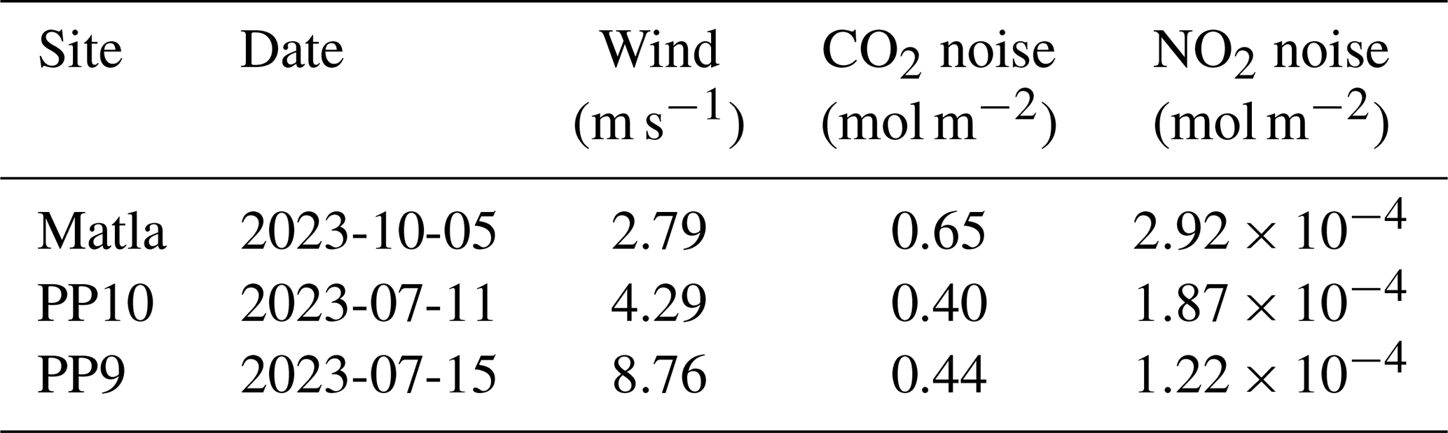
Notes: CO₂ and NO₂ noise values represent the standard deviation of background pixels in each scene, estimated from the EnMAP data as Borger et al. (2025) did not provide retrieval error estimates. These values likely underestimate true measurement uncertainty due to destriping and smoothing preprocessing applied by Borger et al. (2025).

Table 3 Emission estimates from Borger et al. (2025), original and reconstructed CO₂ fluxes, and reconstruction parameters with uncertainties.

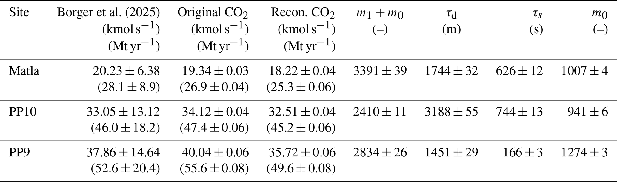
Notes: m₁+m₀ is the apparent CO₂ $/$ NO₂ source ratio, τ_d is the spatial decay scale, τ_s is the effective chemical timescale obtained by converting τ_d using wind speed, and m₀ is the background ratio. Values from Borger et al. (2025) represent cross-sectional flux estimates averaged over 10 km downwind distance for comparison with IME results. Uncertainties on reconstructed fluxes represent formal error propagation of measurement noise only and do not account for systematic errors or preprocessing-induced error correlations (see text).

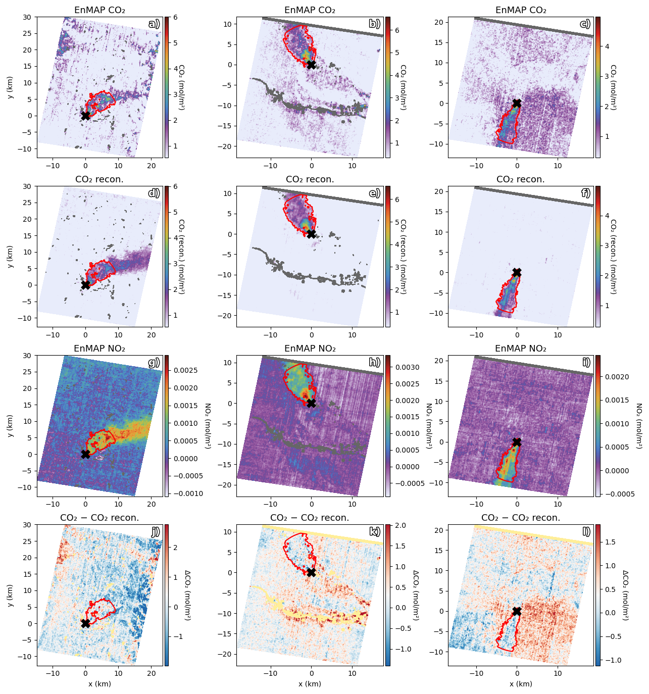
Figure 8 Application of the CO₂–NO₂ plume reconstruction method to EnMAP hyperspectral observations at 30 m spatial resolution over three industrial targets: Matla power plant, Mpumalanga, South Africa (5 October 2023; a, d, g, j), PP10 power plant near Riyadh, Saudi Arabia (11 July 2023; b, e, h, k), and PP9 power plant near Riyadh, Saudi Arabia (15 July 2023; c, f, i, l). First row (a–c): original EnMAP CO₂ retrievals showing plume structures with substantial noise and surface-related artifacts. Second row (d–f): reconstructed CO₂ fields, exhibiting reduced noise and smoother plume patterns. Third row (g–i): EnMAP NO₂ retrievals with inherently lower noise than CO₂ but some remaining artifacts, particularly visible in panel (i). Fourth row (j–l): differences between original and reconstructed CO₂ fields, highlighting the noise reduction and artifact mitigation achieved by the CO₂–NO₂ plume reconstruction. Emission estimates (original vs reconstructed): Matla: 19.34 kmol s⁻¹ (26.9 Mt yr⁻¹) vs 18.22 kmol s⁻¹ (25.3 Mt yr⁻¹); PP10: 34.12 kmol s⁻¹ (47.4 Mt yr⁻¹) vs 32.51 kmol s⁻¹ (45.2 Mt yr⁻¹); PP9: 40.04 kmol s⁻¹ (55.6 Mt yr⁻¹) vs 35.72 kmol s⁻¹ (49.6 Mt yr⁻¹). The red line indicates the plume mask used and the source location is indicated by the black x.

Figure 8 shows application of both masking and reconstruction approaches to the three sites. Row (a–c) displays original EnMAP CO₂ retrievals with clear plume structures but substantial noise and surface artifacts. Row (d–f) shows reconstructed CO₂ fields after CO₂ $/$ NO₂ reconstruction, exhibiting smoother plumes with reduced interference. Row (g–i) shows NO₂ retrievals with lower noise but some remaining artifacts. Row (j–l) displays differences between original and reconstructed CO₂ fields, highlighting noise and bias reduction achieved through the ratio-based approach. As demonstrated earlier, however, this visual noise reduction does not translate into a reduced error on the retrieved emission flux compared to using the original CO₂ field directly. Table 3 compares emission estimates and retrieved reconstruction parameters across the three sites. We note that Borger et al. (2025) used the cross-sectional flux method and reported maximum values within 10 km from the source, methodologically different from our IME method. We averaged their cross-sectional flux estimates over the 10 km downwind range to obtain representative values more comparable to spatially integrated IME results.

For Matla and PP10, emissions from CO₂ measurements with NO₂ masking (26.9 and 47.4 Mt yr⁻¹) and reconstructed fields (25.3 and 45.2 Mt yr⁻¹) agree well with averaged published values (28.1 and 46.0 Mt yr⁻¹). For PP9, CO₂ with NO₂ masking yields 55.6 Mt yr⁻¹ and the reconstructed field gives 49.6 Mt yr⁻¹, both consistent with the averaged published value of 52.6 Mt yr⁻¹. These results demonstrate that both masking and ratio-based reconstruction are applicable to real EnMAP measurements, successfully reproducing previously published emission estimates. Retrieved reconstruction parameters provide additional insight into plume chemistry and atmospheric conditions. The apparent CO₂ $/$ NO₂ source ratio (m₁+m₀) is highest for Matla (3391), while the two Riyadh power plants exhibit similar values (PP10: 2410, PP9: 2834). These differences may reflect variations in combustion efficiency, fuel composition, or flue gas treatment, though they must be interpreted cautiously due to the resolution-dependent biases discussed in Sect. 5 (bias >25 % expected at finite spatial resolution).

The spatial decay parameter τ_d shows substantial variation: Matla exhibits 1744 m, PP10 shows 3188 m, and PP9 displays 1451 m. When converted to temporal scales using observed wind speeds (Table 2), PP9 exhibits the fastest effective chemical timescale (${\mathit{\tau }}_s={\mathit{\tau }}_{\mathrm{d}}/U=\mathrm{166}$ s), whereas for Matla and PP10, τ_s values are similar with τ_s=626 and 744 s, respectively. The faster evolution of the CO₂ $/$ NO₂ ratio, indicates different chemical boundaries for the PP9 plume compared to the other two plumes. The background ratio m₀ also varies across sites. Again, Matla and PP10 show similar results with m₀=1007 and 941, respectively, whereas PP9 deviates from this with m₀=1274. This supports our conclusion based on τ_s, although we are aware that a more detailed chemical analysis is required to interpret the results. The large spread in τ_s across sites (166–744 s) likely reflects differences in boundary-layer turbulence intensity: stronger turbulence entrains background O₃ into the plume more rapidly, shortening the effective NO → NO₂ timescale. The notably short τ_s at PP9 (166 s, close to the clean-air theoretical minimum of ∼ 70 s) is consistent with its high wind speed and vigorous mixing, whereas the longer timescales at Matla and PP10 suggest more sustained O₃ depletion under calmer conditions. Boundary-layer turbulence diagnostics from atmospheric reanalysis products (e.g., CAMS) could be used to test this interpretation quantitatively, but this is beyond the scope of the present study. These results from EnMAP suggest that all the chemistry parameters retrieved from the data remain interpretable even in real EnMAP observations when combined with ancillary wind information, despite complexities from finite spatial resolution and retrieval artifacts.

Quantitative error estimation in EnMAP data is severely limited by preprocessing applied to the products provided by Borger et al. (2025). Input noise estimates from background pixels likely underestimate true uncertainties due to smoothing and destriping that introduce spatial correlations. Consequently, our analytically propagated errors (0.04–0.06 kmol s⁻¹, or approximately 0.1 % relative uncertainty) appear unrealistically small compared to published uncertainties from Borger et al. (2025) (6.38–14.64 kmol s⁻¹, or approximately 20 %–30 % relative uncertainty). Our tabulated uncertainties should be regarded as lower bounds reflecting only propagated measurement noise under assumptions of perfect functional form and error-free ancillary data, not accounting for systematic errors, model limitations, or preprocessing-induced correlations.

We note that our uncertainty analysis focuses on measurement noise and co-location errors, and does not include wind speed uncertainty. Wind speed enters the IME estimate linearly through the transit time $t_{\mathrm{trans}}=L/U$, so errors in the effective wind speed translate directly to proportional errors in the flux: a 30 % error in wind speed yields a 30 % error in the inferred emission rate. Wind speed uncertainty is often the dominant error source in operational satellite-based emission quantification (e.g., Varon et al., 2018; Kuhlmann et al., 2019).

A clear limitation is that reconstruction assumes NO₂ measurements are free of artifacts. Any spurious features in NO₂ – such as striping or calibration errors – are directly imprinted onto reconstructed CO₂ fields through the ratio multiplication (Eq. 12), making reconstruction accuracy highly sensitive to NO₂ data quality. This is evident in Fig. 8, particularly panel (i), where remaining NO₂ artifacts propagate into the reconstructed CO₂ field. Nonetheless, successful application to EnMAP observations demonstrates practical feasibility of the CO₂ $/$ NO₂ synergy approach on real satellite data. Emission estimates agree with independent published results, and chemistry parameters exhibit physically reasonable values with systematic site-to-site variations. For TANGO, with optimized instrument design, consistent measurement characteristics, lower noise levels, and availability of full retrieval error covariances, we expect more robust performance and reliable uncertainty quantification when complete error propagation is applied. The method is ready for deployment in TANGO and other multi-species satellite missions including GOSAT-GW and CO₂M.

6 Conclusions

We present a CO₂–NO₂ synergy method for the TANGO mission and similar satellite platforms providing co-located observations of both species, including EnMAP, GOSAT-GW, and CO₂M mission, and demonstrate its performance on both large-eddy simulations and real EnMAP observations. The method addresses a fundamental challenge in high-resolution greenhouse gas monitoring: Measured CO₂ plume enhancements suffer from substantial measurement noise, whereas NO₂ observations exhibit much higher signal-to-noise ratios over the same industrial facilities. The primary value of NO₂ synergy lies in plume detection and masking. By using NO₂ observations to define spatial masks identifying plume extent, then integrating CO₂ within these masks, emission precision improves by approximately a factor of two relative to analyzing CO₂ without NO₂ guidance. Across emission strengths of 2.0, 2.5, 5.0, and 12.5 Mt yr⁻¹, the masking approach achieves total emission precision of 18.5 %, 14.0 %, 7.6 %, and 3.4 %, respectively, under TANGO-like conditions. Critically, masking exhibits superior bias characteristics for weak sources: at the TANGO detection limit of 2.5 Mt yr⁻¹, masking shows −8.1 % bias. Below 2.5 Mt yr⁻¹, both approaches show substantial biases exceeding 15 %, in agreement with the reported operational detection limit (Landgraf and Veefkind, 2025).

Our second approach – CO₂ $/$ NO₂ ratio reconstruction – fits an exponential model to the observed ratio and generates smoothed CO₂ fields. Despite producing visually cleaner fields with reduced pixel-scale noise, reconstruction does not improve emission precision relative to masking. This counter-intuitive finding has a fundamental explanation: reconstruction transforms uncorrelated pixel noise into spatially correlated errors affecting larger plume areas coherently. When integrating across the entire plume, these correlated errors dominate the error propagation, offsetting any benefit from reduced pixel-scale noise. We demonstrate that neglecting spatial error correlations – using only diagonal covariance matrix elements – underestimates true emission uncertainties by factors exceeding 60. This finding applies generically to any method combining CO₂ and NO₂ through smoothing, regularization, or reconstruction: studies claiming emission uncertainty reduction through synergistic multi-species approaches must provide complete error covariance matrices to prove genuine precision improvement rather than merely redistributing errors across spatial scales. Both masking and reconstruction remain robust to realistic TANGO operational constraints. Spatial grid misalignments up to 150 m introduce biases below 2 %. Temporal separations up to 60 s produce emission biases below 2 %, and emission estimates remain acceptable for temporal offsets up to 2–3 min.

While reconstruction does not reduce emission uncertainty, its primary value lies in atmospheric chemistry characterization. The method retrieves three parameters describing plume chemical evolution: the spatial decay scale τ_d, the apparent source ratio m₁+m₀, and the background ratio m₀. The spatial decay parameter exhibits the clearest physical interpretation: retrieved values of 2100–2300 m substantially exceed TANGO's 300 m instrumental resolution, confirming representation of genuine atmospheric processes. When divided by wind speed, τ_d converts to an effective chemical timescale τ_s characterizing NO→NO₂ oxidation rates, providing a direct observation-based measure of plume chemistry comparable across facilities and atmospheric conditions. The apparent source ratio m₁+m₀ is biased by more than 25 % at TANGO's 300 m resolution because CO₂ and NO₂ form plumes with different spatial structures near the source. The background ratio m₀ should only be interpreted as a CO₂ $/$ NO₂ ratio and an extension to a more useful CO₂ $/$ NO_x ratio remains difficult. Despite these interpretational constraints, all three parameters can provide useful information on the NO_x chemistry within an emission plume and exhibit systematic behavior across emission strengths and atmospheric conditions. The quality of the chemistry parameter depends critically on emission strength. Using simulated TANGO observations for CO₂ emissions of 2.0 and 2.5 Mt yr⁻¹, parameters show uncertainties exceeding 70 %, precluding interpretation. At 5.0 Mt yr⁻¹, parameters become interpretable with 15 %–30 % uncertainties. At 12.5 Mt yr⁻¹, robust retrieval is achieved with 6 %–10 % uncertainties, enabling quantitative chemistry characterization.

Application to three EnMAP satellite observations demonstrates real-world feasibility. Emission estimates from both masking and reconstruction agree well with previously published values, and retrieved chemistry parameters exhibit physically reasonable values with systematic site-to-site variations. The effective chemical timescale of the NO→NO₂ conversion is in the range 166–744 s, confirming physically meaningful characterization. Quantitative error assessment is limited by preprocessing applied to EnMAP products, but successful application confirms operational readiness.

By observing more than 10 000 facilities annually, TANGO will give us the opportunity to build an unprecedented database of site-specific chemistry parameters spanning diverse emission sources and atmospheric conditions. This database could support more robust emission analyses through empirical chemistry constraints, improve NO_x emission estimates from NO₂-only missions, and enable machine learning models predicting chemistry parameters from meteorology and source characteristics. Furthermore, the derived chemistry parameters can be systematically applied to NO₂ retrievals from missions lacking CO₂ observations, enabling indirect CO₂ emission estimates through empirically-constrained relationships between NO₂ and CO₂ sources. For operational emission estimates from TANGO CO₂ and NO₂ observations, we recommend NO₂-based plume masking approach for CO₂ emission quantifications with computational simplicity, superior bias characteristics for weak sources, and straightforward uncertainty propagation. This work highlights the importance of rigorous uncertainty quantification in multi-species synergy methods: a complete error covariance matrix accounting for spatial correlations is needed to demonstrate whether a given approach achieves genuine precision improvement in emission estimates. The CO₂–NO₂ synergy approach is validated, robust to operational constraints, and ready for TANGO deployment.