disdrodb: an open-source Python package for standardized processing, sharing, and analysis of disdrometer data

Disdrometers are specialized sensors designed to measure key properties of falling hydrometeors. Their observations are essential for characterizing precipitation particle size distributions (PSDs) and support a wide range of applications, including precipitation microphysics research, the development and evaluation of remote-sensing precipitation retrievals, and the modelling of microwave signal propagation through the atmosphere for telecommunication systems. However, the broader use of disdrometer data is hindered by limited access to existing datasets, heterogeneous raw data formats, and the lack of standardized, reproducible processing workflows.

This article presents the DISDRODB infrastructure and the associated open-source Python package disdrodb, a community framework for standardized sharing, processing, and analysis of disdrometer data. DISDRODB combines a centralized metadata archive with a decentralized data-sharing model, allowing institutions to retain control of raw data while making their datasets globally discoverable and straightforward for users to access and download through a common interface. The disdrodb software converts heterogeneous raw measurements into analysis-ready products through a modular three-level pipeline: L0 for standardized ingestion and formatting into netCDF4, L1 for temporal resampling, quality control, and hydrometeor/precipitation-type classification, and L2 for derivation of PSD integral parameters, parametric PSD model fitting, and simulation of polarimetric radar variables at multiple frequencies.

The framework provides a transparent, configurable, and reproducible open-source workflow for disdrometer data processing, with scalable execution from local environments to distributed computing systems. It also supports automatic generation of summary diagnostics for scientific analysis and is built on a modular, flexible architecture designed for community-driven extensions.

DISDRODB lowers barriers to both data access and analysis by enabling straightforward discovery and download of disdrometer datasets alongside reproducible processing workflows, thereby supporting large-sample studies of PSD variability, improved disdrometer intercomparison, and broader use of disdrometer observations in atmospheric science and remote sensing.

1 Introduction

Precipitation is intermittent and highly variable in space and time. It occurs in many forms, with different amounts, phases, and hydrometeor types. The phase of precipitation – whether it falls as rain, hail, snow, or mixed – has far-reaching natural and societal implications: it governs seasonal water availability through its influence on snowpack accumulation and melt (Mankin et al., 2015; Berghuijs et al., 2014; Harpold et al., 2017; Han et al., 2024), affects soil moisture and ecosystem dynamics (Trujillo et al., 2012; Harpold and Molotch, 2015; Rixen et al., 2022; Choler et al., 2025), and modulates natural hazards such as flooding (McCabe et al., 2007; Berghuijs et al., 2016, 2019; Blöschl, 2022), icing, and avalanches (Schweizer et al., 2003, 2021). It also critically impacts human activities, including road, rail, and air transportation (Norrman et al., 2000; Gultepe et al., 2019). While the phase and type of precipitation can be monitored using ground networks of present weather sensors, catching-type precipitation gauges, commonly known as pluviometers or rain gauges, have historically been used to monitor precipitation amounts (Lanza and Vuerich, 2009; Strangeways, 2010; Kidd et al., 2017; Su et al., 2026).

Commercial catching-type gauges are, however, not sensitive to light precipitation and must be equipped with heating devices to measure solid precipitation. Tipping bucket gauges report a measurement only after the bucket collects a given amount (typically 0.1 or 0.2 mm of water), depending on the sensor type. This means that a minute with precipitation rates typically below 6 or 12 mm h⁻¹ goes undetected or is reported with a delay only when the bucket gets filled. Evaporation within the bucket can further reduce the measured amount, especially during light or intermittent precipitation (Sevruk, 1974; Dunn et al., 2025). In some cases, the collected water may completely evaporate before the bucket tips, and the event may never be recorded. As a result, a 10 min precipitation (drizzle) event with an average intensity typically below 0.6 or 1.2 mm h⁻¹ may remain unrecorded. Additionally, tipping bucket gauges exhibit mechanical limitations at high rainfall intensities and dynamic calibration of the instrument is therefore recommended (Marsalek, 1981; Humphrey et al., 1997; Lanza and Stagi, 2009; Shedekar et al., 2016; Segovia-Cardozo et al., 2021).

Weighing precipitation gauges are generally more sensitive than tipping-bucket gauges, have a larger collection area, require less maintenance, but are typically configured to report accumulated precipitation amounts every 5 or 10 min, or at longer time intervals (Leeper et al., 2015; Saha et al., 2021). High-frequency measurements, such as 1 min accumulations, require additional processing to filter out signal noise (Ross et al., 2020; Filipovic, 2025). Like other catching-type gauges, they do not provide information about the phase or hydrometeor type and are known to underestimate precipitation in the presence of strong wind (Pollock et al., 2018; Kochendorfer et al., 2017; Cauteruccio et al., 2024).

Disdrometers are non-catching instruments designed to measure the size and number of hydrometeors as they impact or pass through a sensing area (Joss and Waldvogel, 1967; Löffler-Mang and Joss, 2000). Some also measure particles' fall speeds, providing additional information useful to infer hydrometeor types and precipitation phase (Kathiravelu et al., 2016; Lanza et al., 2021). Disdrometers are capable of detecting very light precipitation, with a sensitivity threshold below 0.01 mm h⁻¹ for 1 min measurement intervals (Rees and Garrett, 2021), and unlike catching-type gauges, they provide the complete precipitation particle size distribution (PSD).

The PSD describes the number concentration and size distributions of hydrometeors in a volume of air. The characterization of PSDs is crucial for improving and evaluating microphysical and radiative transfer parameterization schemes in numerical weather prediction models (Seifert and Beheng, 2006; Morrison and Grabowski, 2007; Abel and Boutle, 2012; Yang et al., 2019; Dolan et al., 2023; Niquet et al., 2024), as well as for advancing understanding of microphysical precipitation processes (Morrison et al., 2020). PSD data also help constrain precipitation-driven land surface interactions, such as canopy interception (Levia et al., 2017) and soil erosion (Serio et al., 2019), and impacts on human-built infrastructure, e.g., the erosion of wind turbines (Bech et al., 2022).

PSD measurements are also essential for realistically modelling propagation of optical, infrared, and microwave signals through the atmosphere, a critical requirement for both ground-based and spaceborne telecommunication systems and for atmospheric remote sensing applications (Hogg, 1968; Ulbrich and Atlas, 1985; Bradley et al., 2000; Uijlenhoet et al., 2011; ITU-R, 2025). PSD information enables accurate simulations of precipitation-induced signal attenuation, which can be exploited opportunistically for rainfall estimation using commercial microwave links and satellite downlink signals (Messer et al., 2006; Leijnse et al., 2007; Overeem et al., 2013; Giannetti et al., 2017; Uijlenhoet et al., 2018; Chwala and Kunstmann, 2019; Zhang et al., 2023; Nebuloni et al., 2025; Graf et al., 2025). Knowledge of the PSD also supports modelling hydrometeors' microwave emission and scattering, which shape the radiometric signatures measured by passive microwave radiometers (Bennartz and Petty, 2001; Kneifel et al., 2010; Eriksson et al., 2018). In addition, simulations of the reflectivity and polarimetric variables that weather and cloud radars would observe for a given PSD provide the foundations for developing and evaluating precipitation-retrieval algorithms, radar forward operators and data assimilation systems for both ground-based and spaceborne radar systems (Ryzhkov et al., 2011; Zeng et al., 2016; Wolfensberger and Berne, 2018; Fielding and Janisková, 2020; Kotsuki et al., 2023). Disdrometer measurements also contribute to radar calibration and validation activities (Frech et al., 2017; Chen et al., 2021; Steinert et al., 2021; Deng et al., 2025).

The spatial and temporal structure of the PSD, from local to global scales, is key to understanding precipitation variability. Although this remains an active area of research (Uijlenhoet et al., 2003; Tokay and Bashor, 2010; Jaffrain et al., 2011; Tapiador et al., 2010; Raupach and Berne, 2016b, a; Tokay et al., 2016, 2017; Dolan et al., 2018; King et al., 2025), progress is constrained by the limited spatial and temporal coverage of existing datasets, which hampers a comprehensive characterization of PSD behavior and its links to microphysical, dynamical, and thermodynamic processes (Kumjian and Ryzhkov, 2012; Dawson et al., 2015).

Historically, disdrometers were mainly deployed during short-term field campaigns to improve the understanding of precipitation processes and small-scale variability. With the advent of commercial instruments, their use has expanded to operational observation networks, where they serve as present weather sensors (Blahak et al., 2025) or as backup rain gauges (Petan et al., 2025). In recent years, national and international initiatives have fostered the creation of national disdrometer networks (Adirosi et al., 2023; Petan et al., 2025; Pickering et al., 2019; Blahak et al., 2025) and the installation of sensors at long-term atmospheric observatory sites (Mather and Voyles, 2013; Stevens et al., 2016; Tokay et al., 2016; Laj et al., 2024; Flynn et al., 2026). Several of these sites now provide multi-year datasets, in some cases extending up to a decade of continuous measurements with only minor interruptions.

However, research and modelling of PSDs continue to encounter multifaceted challenges. The scarcity of easily accessible public disdrometer datasets has limited research aimed at unraveling the complex nature of precipitation PSDs (Gatlin et al., 2015; Dolan et al., 2018; Duncan et al., 2019; Ignaccolo and Michele, 2022; King et al., 2025) and has caused remote sensing precipitation algorithms to rely on a priori assumptions about the functional form of the PSD. These assumptions limit the ability to represent the full range of plausible solutions and introduce bias in the precipitation retrievals (Liao and Meneghini, 2013; Duncan et al., 2019; Ladino-Rincon et al., 2025).

Equally daunting is the diversity of sensors, recording conventions, and processing practices adopted by institutions during field deployments. Each institution measures a distinct set of variables and stores observations in heterogeneous text or binary formats, often with little resemblance to one another. This lack of standardization is a barrier to the sharing and long-term management of PSD observations.

Large-sample studies therefore require substantial time and effort to locate, access, review, and harmonize heterogeneous datasets into a consistent format before starting the analysis. Moreover, although some open-source efforts exist (Hardin and Guy, 2014; Leinonen, 2014), the lack of widely adopted and consistently maintained software for standardized disdrometer data processing continues to limit research reproducibility and productivity, thereby constraining the number of large-scale studies. The capabilities and limitations of these instruments are not yet fully characterized either, partly due to the proprietary nature of manufacturers' internal processing algorithms and as a result of the continued scarcity of publicly available data.

With the DISDRODB infrastructure and the software described in this manuscript, we aim to address some of these challenges. The platform provides a unified framework for the systematic sharing, standardization, and processing of disdrometer data. It includes a metadata archive listing all available stations and supports a decentralized data infrastructure, allowing each institution to share their datasets through their preferred dissemination platform. The accompanying Python software enables users to easily access data from selected stations, automatically convert raw measurements into a common standardized format, apply consistent quality control and filtering procedures, compute PSD integral parameters, simulate radar observables and specific attenuation from PSDs, and create summary figures and tables for each station. This automated and customizable processing chain ensures unified and reproducible data handling from collection to public release.

DISDRODB promotes open, transparent, and community-based research practices. It allows scientists to focus on scientific analysis rather than on time-consuming tasks such as data discovery, wrangling, and processing. The resulting global database opens new opportunities for PSD research, advances in (ground-based and spaceborne) remote sensing retrievals, and improved characterization of disdrometer uncertainty and accuracy. The modular architecture of the disdrodb software presented in this manuscript enables users to extend the software with new quality-control procedures, filters, processing chains, products, use individual modules independently, and contribute improvements back directly to the community through the open-source framework.

The manuscript is organized as follows. Section 2 introduces the disdrometer measurement procedures, their characteristics, main limitations, and sources of uncertainty. Its purpose is to provide readers with the essential background needed to correctly interpret and analyze disdrometer data. Section 3 presents the DISDRODB infrastructure, including the metadata archive, the decentralized data archive, the data contribution mechanism and the disdrodb software workflow used to generate the DISDRODB products. Sections 4, 5 and 6 describe in detail the Level 0 (L0), Level 1 (L1), and Level 2 (L2) software processing chains, respectively. The L0 chain converts raw data into a standardized netCDF4 format (Unidata, 2025). The L1 chain resamples data at the desired temporal resolution, performs quality control and identifies precipitation phase and hydrometeor types using the raw particle spectra. The L2 chain computes integral PSD parameters (Sect. 6.1), fits custom models to the observed PSDs (Sect. 6.2), and simulates radar variables at selected frequencies (Sect. 6.3). All mathematical definitions are provided in Appendices A, B, C, D and E.

2 Disdrometer measurements: principles, characteristics, and uncertainties

Disdrometers are point instruments that measure the size and fall velocity of individual falling hydrometeors. They count particles impacting or traversing their sensing volume during a given measurement interval. The sensing volume must be large enough to detect a sufficient number of sparsely distributed large drops, yet small enough to minimize cases where multiple particles cross (or impact) the sensing volume simultaneously. Disdrometers can be classified according to their measurement principle as impact, optical, video, or radar (Lanza et al., 2021), with optical disdrometers accounting for the majority of deployments worldwide. The accuracy of their measurements depends on the instrument's physical design, sensing characteristics and underlying assumptions, as well as its installation setup, environmental conditions, and external interferences. The magnitude of these effects varies by sensor type. Although advanced camera-based disdrometers can track several particles at once (Barthazy et al., 2004; Newman et al., 2009; Garrett et al., 2012; Testik and Rahman, 2016; Maahn et al., 2024; Shi et al., 2025), the instruments considered in this manuscript (see Table 1) cannot reliably separate overlapping signals, which leads to biased estimates of particle size and fall velocity. Detected particles are categorized into discrete size and fall velocity classes, forming a two-dimensional matrix commonly referred to as the disdrometer raw spectrum, which represents the fundamental measurement from which all estimated PSD quantities are derived. The software presented in this work currently supports the processing of impact and optical disdrometers. Its modular design, however, allows for future integration of additional instrument types. Table 1 summarizes the main characteristics of the currently supported sensors.

Table 1 Characteristics of the disdrometers supported by DISDRODB. L, W, D, and H denote the nominal length, width, diameter, and height of the sensing area, respectively. The reported D_max and V_max values correspond to the lower bounds of the last diameter and fall-velocity classes, respectively. The symbol “–” indicates parameters that are not applicable, while “n/a” denotes information not available or not disclosed by the manufacturer.

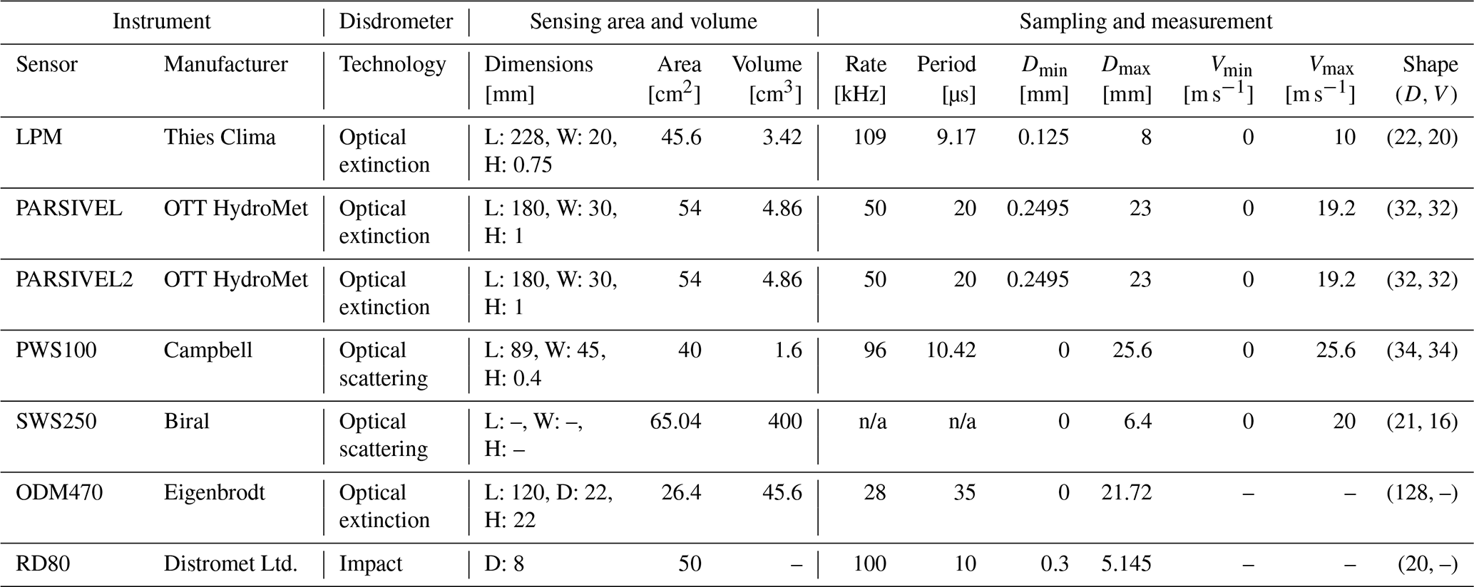
In the following subsections, we describe the operating principles of impact and optical disdrometers, highlighting the characteristics, limitations, and processing uncertainties associated with each type. This overview provides the essential background needed to correctly interpret and analyze disdrometer measurements and the outputs of the processing chain presented in this manuscript.

2.1 Impact disdrometers

Impact disdrometers characterize the PSD by counting and measuring the force produced by the hydrometeors striking the sensor surface. Each particle impact causes a small displacement of the sensor cover, generating a mechanical vibration that is converted into an electrical signal. The signal is related to the particle's kinetic energy and used to estimate the particle size. The kinetic energy of a particle is directly related to its mass and fall velocity. Impact disdrometers, however, do not directly measure particle fall velocity.

For raindrops, assuming constant water density and a known mass-diameter relationship, the use of a terminal fall-velocity model allows for a reliable estimate of particle size from the measured impact energy. In contrast, snow particles exhibit a wide range of shapes, densities, masses, and fall velocities, making their impact response highly variable and preventing a reliable estimation of particle size. Therefore, impact disdrometers such as the Joss-Waldvogel Disdrometer (Joss and Waldvogel, 1967, hereafter RD80) can only be reliably used to characterize the raindrop size distribution (DSD).

The RD80 disdrometer detects raindrops within the 0.3–5.5 mm diameter range, with drops larger than 5.5 mm all counted in the largest size bin. This limitation arises because the variation in raindrop terminal fall velocity, and consequently in kinetic energy, becomes very small for drops larger than 5 mm (see Fig. B1 in the Appendix), reducing the instrument's ability to distinguish between large drop sizes.

At the lower end of the spectrum, undersampling of small drops has been reported particularly during heavy rainfall when multiple drops impact the sensor surface quasi-simultaneously (Tokay et al., 2003, 2005). This issue, known as the dead-time effect, occurs when the impact of a large drop causes the sensor cone to vibrate. During these vibrations, smaller raindrops arriving within the next few milliseconds cannot be recorded. As a result, only the largest drop is registered, leading to an undercount of smaller drops (Sauvageot and Lacaux, 1995; Uijlenhoet et al., 2002).

Over time, prolonged exposure to solar radiation and repeated contact with rain gradually reduce the elasticity of the sensor surface cover, further lowering sensitivity to small drops. Additionally, strong winds and acoustic noise can also alter or mask the impact signal of small raindrops.

Finally, the RD80 relies on a fixed empirical relationship to convert the impact signal into drop size. Raindrops falling at sub-terminal or super-terminal velocities (Montero‐Martínez et al., 2009) are therefore underestimated or overestimated in size, respectively. The resulting effects on inferred DSDs and associated power-law relationships are discussed in Leijnse and Uijlenhoet (2010). In addition, because terminal fall velocity increases with altitude as air density decreases, and this effect is not accounted for in the instrument's internal calibration, raindrop sizes tend to be increasingly overestimated at higher elevations.

2.2 Optical disdrometers

Optical disdrometers measure the light extinction or light scattering of hydrometeors falling through their sensing volume. The measurement principles vary depending on whether they are based on light scattering or extinction. Table 1 reports the characteristics of the optical disdrometers supported by disdrodb.

2.2.1 Extinction-based optical disdrometers

Extinction-based optical disdrometers measure precipitation by detecting the reduction of light intensity caused by hydrometeors passing through a thin laser beam (Hauser et al., 1984; Salles et al., 1998; Löffler-Mang and Joss, 2000) or a homogeneously illuminated volume (Illingworth and Stevens, 1987; Grossklaus et al., 1998; Lempio et al., 2007). Examples of such instruments supported by disdrodb are the OTT PARSIVEL (1 and 2), Thies LPM, and Eigenbrodt ODM470 sensors. In both configurations, a receiver, typically a photodiode, is located in front of the light source to measure the incoming light intensity.

When a particle falls through the beam, the receiver measures a temporary decrease in voltage. The amplitude of this signal reduction is proportional to the particle's horizontal cross-sectional area, while its duration, the particle's residence time (t_residence) within the sensing volume, is related to the particle fall velocity and vertical dimension.

The particle's horizontal size (p_size) is derived from the maximum signal reduction and corresponds to the particle's maximum horizontal dimension. For raindrops, assuming they fall with their axis of symmetry vertically aligned, p_size corresponds to the drop's major axis (A). Assuming a raindrop axis ratio a_r (see Appendix A), the drop minor axis (B) can be obtained as B=Aa_r. The fall velocity can then be estimated as $V=(H+B)/t_{\mathrm{residence}}$, where H represents the thickness of the laser beam or illuminated volume (see Table 1).

For non-spherical particles such as snowflakes or ice crystals, the random orientation and irregular shape of the falling particles make it difficult to relate the measured horizontal size to their actual maximum and vertical dimensions (Battaglia et al., 2010). The complex structure of snowflakes, such as internal air pockets within crystals, and the different extinction properties of ice compared to liquid water, further increase the uncertainty of the particle size estimate.

2.2.2 Scattering-based optical disdrometers

Scattering-based optical disdrometers measure precipitation by detecting the near-infrared light scattered by hydrometeors passing through one or multiple light beams. Light is scattered through a combination of reflection, refraction, and diffraction, with their relative contributions depending on the particle's shape, phase, and refractive index. These instruments record the amplitude and duration of the scattered light pulses generated by each hydrometeor as it crosses the sensing volume. Similar to extinction-based disdrometers, the signal duration provides an estimate of the particle's fall speed, while its size can be derived using two different approaches.

The Campbell PWS100 uses two forward-scatter receivers placed at 20° to the beam, one in a vertical plane and one in a horizontal plane. Since refraction is the dominant scattering mechanism for raindrops, the scattered light reaches the vertical receiver slightly before the horizontal one. This time delay represents the time it takes for a drop to fall a known fraction of its diameter and, when combined with the fall speed, allows the drop size to be determined (Ellis et al., 2006).

Other instruments, such as the Biral SWS-250, VPF-730, and VPF-750, employ two receivers mounted in the horizontal plane: a forward-scatter receiver at 45° and a backscatter receiver at 113°. In this case, the maximum amplitude peak in the signal recorded by the receivers is used to estimate the particle size, while the ratio between forward and backward scattered light provides information on the hydrometeor phase. While for raindrops refraction dominates scattering, for frozen precipitation (e.g., ice pellets, hail, or snow), diffraction and reflection become more significant. Ice particles containing trapped air bubbles or opaque crystalline structures tend to produce stronger backscatter signals, enabling discrimination between liquid and solid precipitation.

2.2.3 Limitations of optical disdrometers

Disdrometer measurements are sensitive to both instrumental limitations and environmental factors. These issues directly affect the accuracy of the retrieved DSD and its integral parameters. Particles that do not fall completely within the sensing volume cause only partial extinction or scattering of the light beam. As a result, they appear smaller than their actual size but with an unrealistically high fall velocity. This phenomenon, known as edge effects in the scientific literature, primarily affects larger drops, which have a higher likelihood of crossing the sensing volume boundaries. The OTT PARSIVEL sensors remove margin fallers from their measurements through the use of two additional photodiodes (Battaglia et al., 2010), whereas other optical disdrometers do not appear to filter out these particles.

Accurate measurement of large drops is also limited by their very low concentration, sparse spatial distribution, and the small sensing area of the instrument, which lowers the probability of detecting them, a limitation commonly referred to as the sampling effect. In addition, disdrometers typically use wider size bins (about 1 mm) for particles larger than 5 mm, and this coarser binning reduces the precision of the reported particle size estimates, an issue known as the quantization effect.

Simultaneous passage of horizontally overlapping particles through the sensing volume can lead to the detection of a single hydrometeor with an overestimated diameter and an underestimated fall speed. Similarly, vertically overlapping particles increase the measured signal duration, resulting in an overestimation of residence time and an underestimated fall velocity. These coincidence effects become more likely as rainfall rate and the number of falling drops increase. Their magnitude depends on the sensor's sampling area, the vertical thickness of the beam, and the sampling frequency.

During intense rainfall, an overestimation of small particle counts may also occur when raindrops impact the instrument housing or sensor surface, fragment, and rebound into the sensing area. This artefact is known as the splashing effect (Pickering et al., 2019; Friedrich et al., 2013).

In the presence of strong horizontal wind, large raindrops can become canted and distorted (Testik and Pei, 2017; Bolek and Testik, 2022; Zheng et al., 2024), appearing narrower than their true size when passing through the sampling area of a disdrometer. This effect leads to a slight underestimation of the size and fall velocity of large drops (Friedrich et al., 2013; Lin et al., 2021). Strong horizontal winds can also modify particle trajectories. Small droplets, which are expected to deviate more than larger drops, may cross the sensing volume at an angle or even horizontally. This may increase their residence time, resulting in an underestimation of fall velocity, and a higher probability of edge effects.

Proper sensor exposure is essential to minimize the effects of turbulence and vertical wind on disdrometer measurements. The instrument should be installed in an open area, away from objects that disturb the normal airflow. As a general guideline, a structure affects the airflow upwind over a distance of about twice its height and downwind over a distance of about six times its height (WMO, 2024). Obstacles such as towers, walls, or nearby instruments can create complex aerodynamic interactions between the airflow, the instrument body, and the approaching hydrometeors. These effects may introduce vertical air motions that modify particle trajectories and bias fall velocity measurements (Kim and Song, 2018; Capozzi et al., 2021). Turbulence also broadens the observed distribution of fall velocities (Testik and Bolek, 2023; Zheng et al., 2024).

Wind is widely recognized as the most significant source of measurement biases. When the wind blows parallel to the sensor, turbulence generated by the airflow around the instrument heads can create updrafts that alter drop trajectories and reduce their fall velocities (Chinchella et al., 2024, 2025). Particles that impact the sensor or are diverted away from the sampling area lead to a significant undercatch and an underestimation of rainfall rate. In contrast, when the wind flows perpendicular to the laser beam, the disturbances are limited, and the wind-induced bias is smaller, typically within 10 %. To mitigate these wind-related biases, future disdrometer designs should aim to include dynamic orientation mechanisms. The OCEANRAIN project has specifically addressed this challenge by equipping its ODM470 sensors with a wind vane that automatically pivots the instrument, keeping the sampling area aligned perpendicular to the local wind direction (Klepp, 2015; Klepp et al., 2018). Similarly, Friedrich et al. (2013) modified PARSIVEL disdrometers by rotating and tilting the sampling area into the wind to avoid artefacts observed during heavy rainfall with strong winds.

Beyond aerodynamic and instrumental biases, disdrometer measurements are also affected by various environmental and operational noise sources. Occlusion of the lenses by spider webs, dew, raindrops, or snow can alter the measurements, as can direct sunlight entering the field of view of the receiver(s). Artificial signals generated during cleaning of the optics, as well as spurious detections from birds, insects, pollen, and other non-precipitation particles, may result in erroneous hydrometeor counts. In cold environments, snow or riming can block the transmitter or receiver lenses, leading to sensor downtime or poor data quality. Blowing snow represents an additional source of noise.

Accurate disdrometer measurements also depend on regular maintenance and periodic recalibration. However, the current lack of standardized calibration procedures contributes to measurement uncertainty both within and between different sensors. This challenge is being addressed through ongoing initiatives such as the INCIPIT project (Baire et al., 2022; Merlone et al., 2022; Chinchella et al., 2026) as well as through European standardization efforts that define metrological requirements and calibration methods for non-catching precipitation sensors (CEN, 2025).

Another major source of inconsistency arises from the proprietary and often undocumented internal processing of the instruments. Although optical disdrometers use the same fundamental detection principles, differences in their physical design, geometry, and internal filtering algorithms lead to deviations in measured quantities. The absence of documentation for key internal processes – including the counting algorithm, the handling of marginal or coincident particles, and the filtering of unrealistic or non-precipitation signals – makes cross-sensor comparison challenging. Firmware changes over time introduce additional uncertainty, further limiting the consistency of long-term DSD monitoring.

The maximum rainfall rates a sensor can measure under extreme conditions are determined by its sampling rate ($A/D$ conversion), its actual processing capacity (maximum number of particles per second), and the presence and size of any temporary buffer used to store particle signals. Unfortunately, manufacturers often do not fully disclose this information.

While the DISDRODB infrastructure and software presented in this study cannot eliminate the inherent instrumental limitations and measurement biases discussed above, it provides a foundation for advancing disdrometer development and DSD research. By offering direct access to previously unavailable data and standardizing all records into a unified, analysis-ready format, the software enables consistent analysis and reproducible workflows. This, in turn, facilitates comparison across instruments, helps identify sensor-specific limitations, and supports large-sample studies of DSD variability.

3 DISDRODB infrastructure

The DISDRODB infrastructure includes a metadata archive, a decentralized data archive and the Python package disdrodb. The system deliberately decouples data discoverability and access, which are centrally managed through the metadata archive, from physical data storage, which remains decentralized and under the control of data providers. Figure 1 illustrates the core components, which are described in detail in the following subsections.

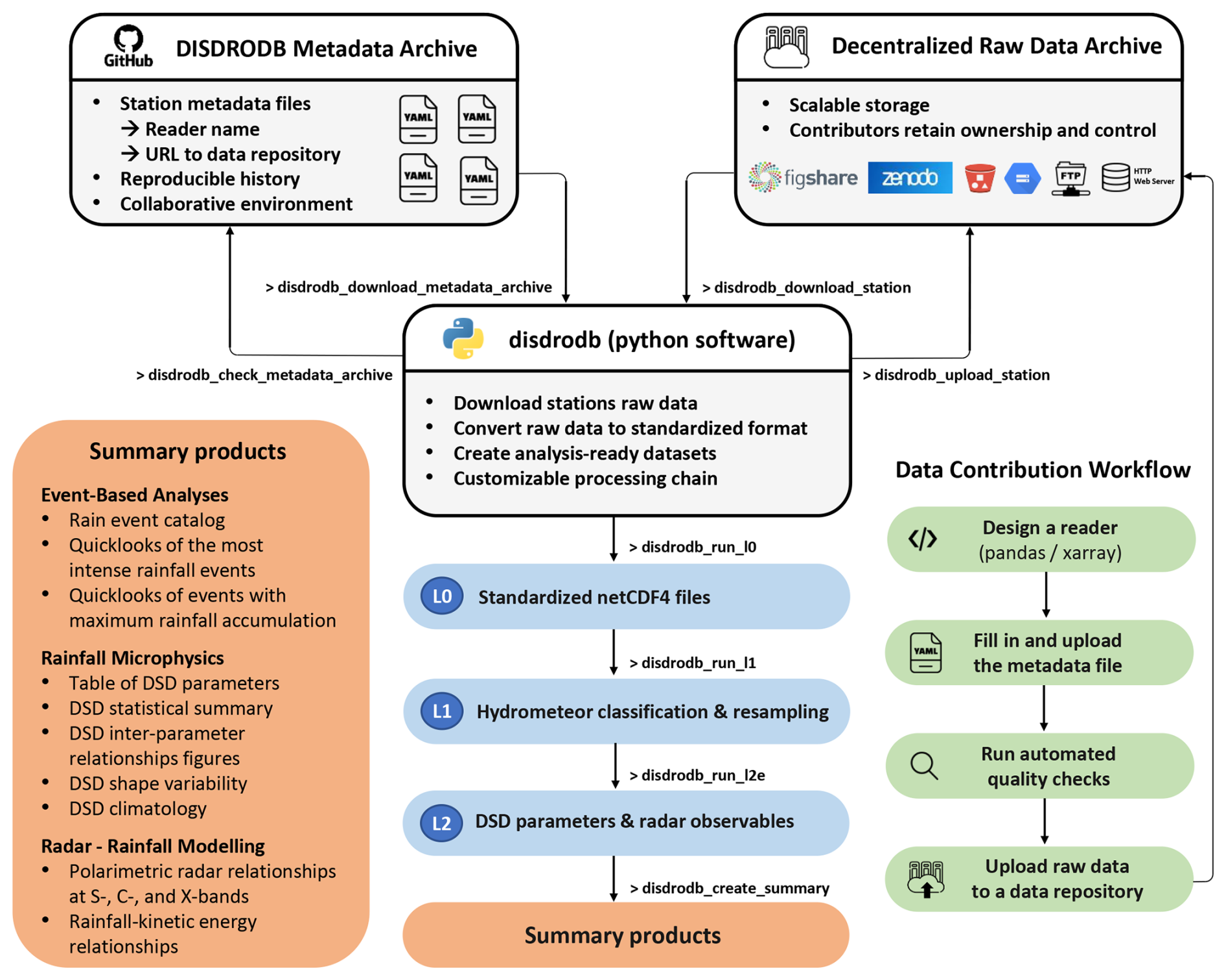
Figure 1 Schematic overview of the DISDRODB infrastructure and processing workflow. The disdrodb Python software interfaces with a centralized metadata archive and decentralized raw data repositories, enabling standardized data ingestion, automated quality control, and the generation of hierarchical, analysis-ready products (L0–L2). The data contribution workflow is illustrated on the right. The left (orange) panel summarizes the figures and tables automatically produced by the software to support scientific analysis. These represent the initial set of products provided by the current version of the disdrodb package and can be extended or complemented with additional products, as users can modify the open-source software.

3.1 DISDRODB Metadata Archive

The metadata archive is hosted on GitHub and serves as a central platform for listing available stations. A station represents an individual disdrometer sensor deployed at a specific location. Each station is described by a metadata file containing standardized fields that specify the instrument details, geolocation, data reader, and the URL to the public data repository where the raw data are shared. Users can also report specific timestamps or periods when sensors malfunctioned – due to environmental interferences such as spider webs, birds, or icing – or produced erroneous records caused by, for example, human intervention, using dedicated issue files. The disdrodb software can automatically exclude these problematic time steps when generating DISDRODB products. GitHub enables community collaboration, allowing continuous improvement of metadata quality, reporting of data issues, and maintaining a transparent, fully reproducible DISDRODB processing chain.

Institutions and contributors may upload station metadata even if the data are not yet publicly available due to policy constraints or embargoes. The DISDRODB metadata archive thus acts as a catalog of all past, present, and future disdrometers, ensuring centralized long-term documentation and improved data findability. An interactive web map is available at https://disdrodb.org (last access: 16 July 2026) to explore the stations, with filtering options based on data availability, deployment status, time period, duration, sensor type, data source, campaign name, and station name.

3.2 DISDRODB Decentralized Data Archive

To encourage data sharing, we recognized the need for a contribution system that is both user-friendly and preserves contributor control and authorship. Therefore, DISDRODB follows a decentralized archive model, in which contributors store their data on their preferred online platform and reference these storage locations in the DISDRODB Metadata Archive. All raw data from a disdrometer station can be uploaded as a ZIP archive to data repositories such as Zenodo or Figshare. Alternatively, the use of institutional web or File Transfer Protocol (FTP) servers allows near-real-time data dissemination and user-side incremental updates of the DISDRODB data archive. In both cases, the URL of the ZIP archive or the server directory, specified in each station metadata file within the DISDRODB Metadata Archive, enables the disdrodb software to automatically access and retrieve the requested data.

By requesting contributors to share only the raw data, DISDRODB removes the time-consuming requirement to convert data into a standardized format and thus simplifies data contributions. This approach differs from other continental or global community datasets that require harmonized data submission (Holben et al., 1998; Baldocchi et al., 2001; Illingworth et al., 2007; Pappalardo et al., 2014; Huuskonen et al., 2014; Saltikoff et al., 2019; Kratzert et al., 2023).

The decentralized archive model respects institutional data governance policies, reduces dependence on a central authority, and lowers the barrier to participation. Institutions retain control and authorship over their data and can autonomously modify, update or withdraw their datasets as needed. This aspect is especially important for organizations such as meteorological agencies, which often operate under strict data governance mandates or legal obligations related to data ownership and sharing. Unlike centralized data archives, DISDRODB does not rely on a single group to accept, collect, maintain, and distribute all data. Instead, the decentralized model fosters collaboration and inclusivity within the research community and promotes open data exchange among users and contributors. Lastly, the decentralized nature of the archive is inherently scalable, allowing it to accommodate increasing volumes of data without structural limitations. It also avoids the costs typically associated with centralized storage solutions, such as expenses for disk capacity and dedicated technical staff, making it a cost-effective and sustainable data management approach.

3.3 DISDRODB data contribution process

The data contribution process to DISDRODB has been designed to be simple and time-efficient for contributors and is supported by comprehensive documentation, including tutorials and examples. The four main steps are outlined below:

1. Design a reader: Data contributors start by crafting a reader tailored to their raw disdrometer data, leveraging the existing reader templates and tutorials. The software already includes hundreds of readers for various instruments and data formats; therefore, in many cases, adding a new dataset requires only minor adaptations of an existing reader. The reader must be added to the dedicated reader directory within the disdrodb software. If the raw data are in text format, the goal of the reader function is to return a pandas.DataFrame (McKinney, 2010), where each row corresponds to a measurement interval. If the raw data are in netCDF4 format, the reader must return an xarray.Dataset (Hoyer and Hamman, 2017). These formats and libraries are widely adopted and well established within the scientific Python ecosystem, ensuring interoperability and long-term usability of the processed data. Variable names must follow the DISDRODB convention, and time must be expressed in UTC and refer to the end of the measurement interval.

2. Fill the metadata: Contributors then fill in a station metadata file and upload it to the DISDRODB Metadata Archive. The metadata file follows a defined structure with mandatory and optional fields. Mandatory fields include the station name, reader name, sensor type, geolocation, and raw data file naming pattern. Optional fields, such as description, authorship, and acknowledgements, can be added at the contributor's discretion.

3. Run the automatic quality screening: At this stage, the DISDRODB automatic screening system rigorously checks the new data, reader, and metadata for compliance with the DISDRODB standards. When producing the DISDRODB L0 products for a station, the system generates a detailed log that lists raw files that are corrupted, empty, or unreadable. Contributors can then remove these files or adjust the reader if needed.

4. Data upload: Contributors upload the station's raw data to their chosen online repository and incorporate the data URL into the station metadata file. To simplify this step, the disdrodb software provides a command-line tool that can automatically upload data to Zenodo, if the user wishes, and update the DISDRODB metadata archive accordingly.

3.4 disdrodb software

The disdrodb software (Ghiggi et al., 2026b) is designed to facilitate fast access to and download of disdrometer raw data and to streamline their subsequent scientific processing. As introduced earlier, Sects. 4, 5 and 6 describe in detail the Level 0 (L0), Level 1 (L1), and Level 2 (L2) processing chains, respectively. In brief, the L0 chain standardizes raw data into netCDF4 format; the L1 chain performs resampling and quality control and identifies precipitation phase and hydrometeor types; and the L2 chain derives PSD parameters, fits statistical models, and simulates radar variables. After completion of the L2 processing, the software can automatically produce summary figures and tables to support data analysis.

disdrodb enables users to download and generate products from each processing chain with only a few terminal commands (see Fig. 1) or Python function calls (see Fig. 2). The software offers three computation modes. In single-process mode, files are processed sequentially, which is useful for debugging and testing. In parallel mode, multiple files are processed simultaneously across processor cores. The third mode uses Dask (Rocklin, 2015) to build computation graphs representing the processing chain operations, enabling lazy, memory-efficient, distributed execution. The progress of parallel and distributed computation can be monitored in real time through the Dask dashboard. Together, these modes provide flexibility from local debugging and analysis to large-scale automated production workflows.

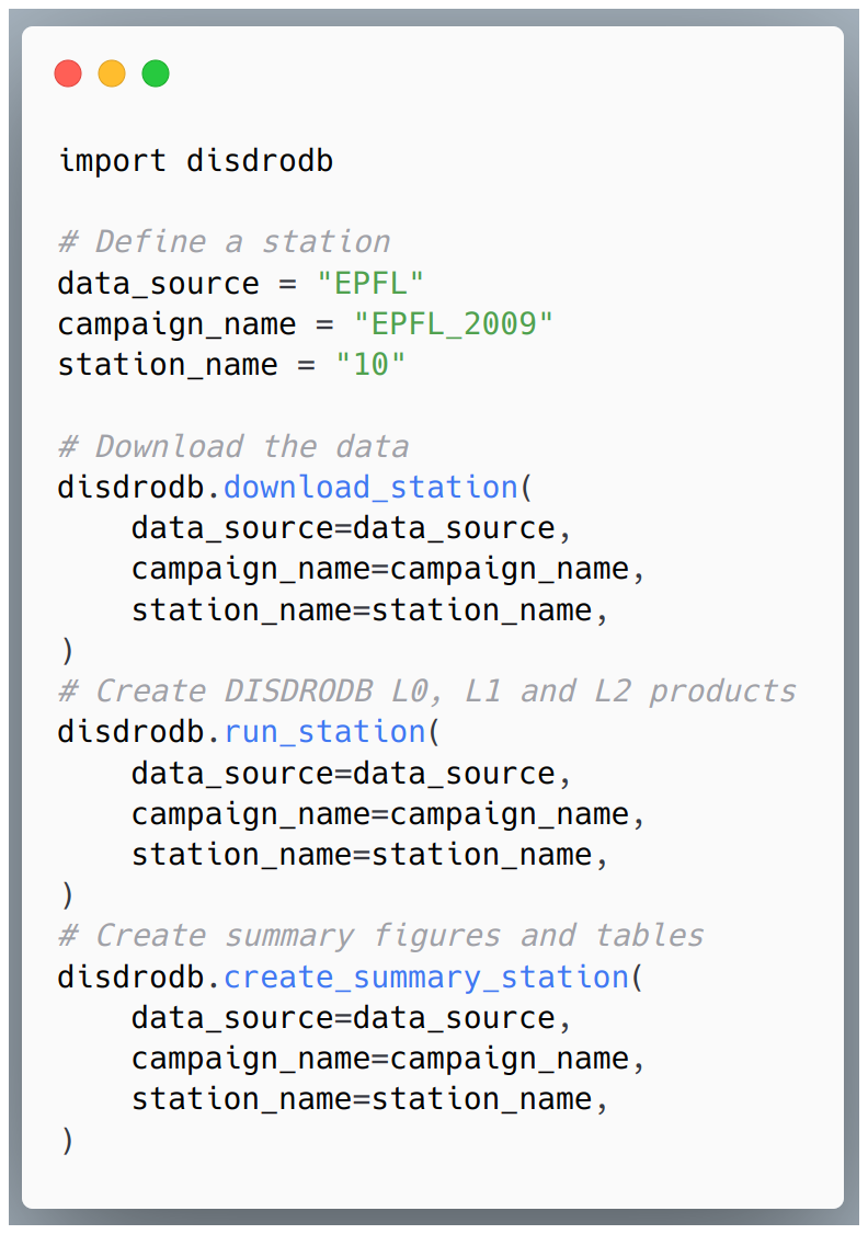
Figure 2 disdrodb Python function calls required to download and generate all DISDRODB products, as well as summary figures and tables, for a given station. Equivalent command-line tools are also available (disdrodb_download_station, disdrodb_run_station, disdrodb_create_summary_station) and are supported on Windows, Linux, and macOS.

The components of the processing chain can also be used independently outside the main pipeline. This allows users to create customized workflows: for example for internal near-real-time product generation or for producing files that comply with institutional data policies and naming conventions. Examples are provided in the online software documentation.

To accommodate the large variety of data formats, disdrometer models, and user requirements, the disdrodb codebase follows a modular design, where each processing chain or software functionality is implemented as an independent module or directory. The software includes two types of editable, human-readable configuration files: sensor configuration files, which define the specific characteristics of each disdrometer model, and product options configuration files, which control the generation of DISDRODB products. This modular design facilitates the integration of new sensor types, algorithms, and models, and supports the development of additional specialized L2 products.

Product configuration files can be easily edited to adjust parameters or add new options. Reasonable defaults are provided, but users can modify settings per sensor type and/or per product temporal resolution. Product archiving is equally customizable. Users can specify the time period for output files (e.g., daily, monthly, yearly, or event-based) and define how data are grouped and stored within subdirectories. Figure 3 provides an example of a product-options configuration file describing the L2E processing chain.

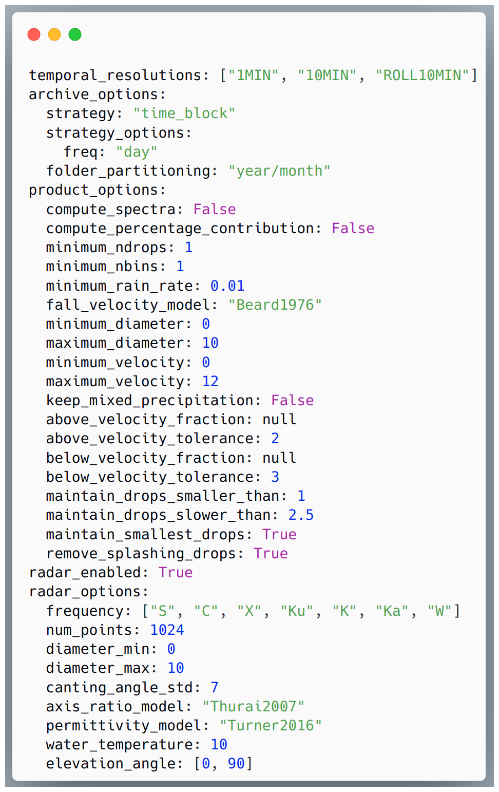
Figure 3 Example of an L2E product global configuration file. The archive options control how output files are stored on disk. The production options allow users to customize the processing chain steps; for the DISDRODB L2E product, this includes filtering of the raw spectrum and selection of time steps to retain or discard (Sect. 6.1). The radar options control the simulation of radar variables (see Sect. 6.3 and Table 6 for more information). Radar frequencies can be specified either in GHz or using IEEE (Institute of Electrical and Electronics Engineers) radar band designations.

To ensure long-term robustness and maintainability, the disdrodb codebase is supported by an extensive automated test suite with high coverage, providing a robust foundation for stable operation and future maintenance. A Continuous Integration (CI) workflow is implemented to regularly run tests and validation checks across multiple operating systems (Windows and Linux), with scheduled executions at least once per month to provide early warnings of potential issues arising from changes in dependencies, operating systems, or the broader Python ecosystem. This approach helps to ensure that the software remains functional, up to date, and compatible with evolving scientific computing environments. In summary, disdrodb provides an automated yet highly configurable processing framework that ensures full flexibility while maintaining traceability and reproducibility from data collection to public product release.

4 DISDRODB L0 products

The DISDRODB Level 0 (L0) processing chain consists of three sub-products – L0A, L0B, and L0C (explained in the following subsections) – which are generated sequentially, starting from the files containing the raw data logged by the disdrometer. All time-varying variables logged by the sensor can be included in the L0A, L0B, and L0C products. Each disdrometer model computes and outputs a specific set of variables and diagnostics; consequently, the content of the raw files and resulting L0 products varies between sensor models and depends on the logging configuration used. disdrodb accepts any subset of logged variables, provided that the raw particle spectrum (i.e., the number of particles per diameter bin, and per velocity bin, if available) and the measurement end time (in UTC) are available. Additional meteorological variables from nearby sensors, if available, can also be included in the L0 products. The main objective of the L0 processing chain is to convert raw data into standardized netCDF4 files with unique time steps and measurement intervals. The uniform L0C data format simplifies scientific analysis and provides a consistent foundation for generating all subsequent DISDRODB products.

4.1 DISDRODB L0A product

The DISDRODB L0A product is generated from the raw text files logged by disdrometers. Raw text files are converted into binary Apache Parquet (Apache, 2026) files using a reader function, typically defined by the data contributor (see Sect. 3.3). This function reads the raw files and returns a dataframe that conforms to DISDRODB standards. Each row corresponds to a measurement time step, and each column to a variable recorded by the sensor, with column names following the DISDRODB naming convention. Variables that represent arrays – such as the raw particle spectrum, mean particle velocity per diameter bin, or particle number concentration – are stored as single-column string entries containing comma- or semicolon-separated values. These arrays are later extracted and reshaped to their correct dimensions in the L0B processing chain. The dataframe produced by the reader is passed to a sanity-check routine that performs a series of cleaning and standardization steps to produce a DISDRODB-compliant L0A dataset. The procedure removes rows where the measurement time is not available, removes duplicated timestamps, filters out time periods flagged as problematic in the issue file, trims spaces from string fields, strips trailing delimiters from array strings, and converts corrupted numeric entries to NaN (Not a Number; the standard floating-point representation for undefined or missing numerical values). Column data types are cast according to DISDRODB definitions, and missing-value flags or out-of-range entries are replaced with NaN. All issues encountered during this process are recorded in the corresponding L0A log file, allowing users to diagnose problems, refine the reader where necessary, or manually correct corrupted raw files if needed. Finally, the dataframe is sorted by time and validated to ensure full compliance with DISDRODB L0A standards.

4.2 DISDRODB L0B product

The DISDRODB L0B product is typically generated from the DISDRODB L0A product. A special case occurs when institutions share raw data only as netCDF4 files; in such cases, the reader function produces the L0B product directly from the raw files, applying the same sanity checks described for the L0A processing chain. In the standard workflow, the L0B chain ingests the L0A dataframe, parses string arrays (e.g., the raw particle spectrum) into multidimensional arrays, and creates an xarray.Dataset with time, diameter, and, if available, velocity dimensions. Coordinate variables defining the bin centers and bounds for diameter and velocity are added, along with station geolocation information (longitude, latitude, and altitude). Each dataset variable is supplemented with Climate and Forecast (CF) convention attributes (Eaton et al., 2024), and variable-specific encodings are applied to minimize disk space usage when the product is written to a netCDF4 file. The metadata fields defined in the station's metadata file are attached as global attributes, complemented by additional Attribute Convention for Data Discovery (ACDD) fields (ESIP, 2015).

4.3 DISDRODB L0C product

The DISDRODB L0C product aims to produce files with fixed time periods (e.g., daily or monthly), unique measurement intervals, and no duplicated time steps. If a disdrometer sensor logs a variable representing the actual measurement interval and this value differs from the expected one(s) specified in the station metadata file, the L0C chain removes the affected time steps. In some logging configurations, raw files may include data from previous days (for instance, due to transmission buffers, temporary storage delays, or manual file handling). When multiple L0B files reflecting these raw data are concatenated, the L0C chain identifies and removes any resulting duplicated time steps. When duplicated time steps contain inconsistent values, a warning is recorded in the product log file, and the conflicting entries are removed. Because some sensors can operate, or have operated, with measurement intervals that vary over time, although this is relatively uncommon, the L0C chain separates the data into distinct xarray datasets, each corresponding to a single measurement time interval. This separation ensures accurate temporal resampling during the subsequent DISDRODB L1 processing stage and prevents the introduction of downstream estimation errors, for example in the computation of the particle number concentration or precipitation rate. Each dataset is then processed independently in the remaining L0C steps.

Once a homogeneous measurement interval has been confirmed, its duration in seconds is stored as a coordinate in the xarray.Dataset. The time axis is corrected, if necessary, to account for drifting seconds. This adjustment aligns small timing offsets – such as timestamps recorded at 00:01, 01:02, or 02:03 when the expected measurement interval is 60 s – to exact multiples of the interval (e.g., 00:00, 01:00, 02:00). The correction typically also enforces that time steps end with 00 s, unless this is incompatible with the defined measurement interval. To assess temporal continuity, a quality-control variable (qc_time) is computed to indicate whether each time step is isolated, has at least one neighboring measurement, or belongs to a continuous sequence. This check also considers continuity across adjacent files or time periods. Finally, a time-step regularity check is logged in the L0C log file. This diagnostic warns about the presence of highly intermittent measurements or recurring irregular time differences between observations, which may suggest that the sensor operated with a measurement interval different from the one expected. This information can be used to correct the expected measurement interval(s) in the station metadata file.

5 DISDRODB L1 products

The DISDRODB L1 processing chain performs temporal resampling of the raw particle size distributions, applies spectrum-level quality control, and classifies the precipitation phase and hydrometeor types. These steps ensure that all disdrometer observations, despite differences in sensor design, sampling frequency, and logging configuration, are homogenized in both temporal resolution and physical interpretation. The following subsections describe the main components of the L1 chain: temporal resampling (Sect. 5.1) and hydrometeor classification (Sect. 5.2), along with their associated quality-control procedures and output variables.

5.1 Temporal resampling

Disdrometer sensors operate at heterogeneous native temporal resolutions, typically between 10 and 60 s, with some networks adopting longer intervals up to 5 or even 10 min. To handle this variability, the DISDRODB L1 processing chain aggregates the raw particle spectra and auxiliary meteorological variables to the temporal resolution specified by the user, constrained to multiples of the native measurement interval. Depending on the research objective, data can be aggregated at 1, 5, or 10 min intervals to represent different spatio-temporal scales of the PSD. To avoid data loss when aggregating over fixed blocks (e.g., 2 min intervals), disdrodb offers a rolling-window resampling option, which increases the number of aggregated samples by performing overlapping integrations (e.g., producing 5 min integrated data every 1 min). A quality-control variable, qc_resampling, reports the fraction of missing time steps within each temporal aggregation window, with values ranging from 0 (no missing data) to 1 (all time steps missing). This information enables users to apply a posteriori filtering and identify potentially biased aggregated estimates.

5.2 Hydrometeor classification

The hydrometeor classification (HC) module analyses the raw particle size-velocity spectrum recorded by disdrometers to identify the dominant hydrometeor type and precipitation phase at each time step. It operates on the raw two-dimensional particle number spectrum (diameter-velocity) and, when available, incorporates auxiliary environmental variables such as air or sensor temperature. Before classification, sensor-specific filters remove noisy bins, typically the first diameter or velocity classes affected by environmental noise and the low sensitivity of the instruments. For disdrometers that do not measure fall velocity (e.g., RD80, ODM470), the HC module is not applied.

Figure 4 illustrates the partitioning of the raw particle size-velocity spectrum, based on Friedrich et al. (2013). The algorithm defines masks for different hydrometeor categories – including drizzle, rain, graupel, hail, snow, and snow grains – using theoretical and empirical fall-velocity-diameter relationships. Each mask isolates the region of the spectrum consistent with the expected velocity-size range of a given hydrometeor type. Because fall velocity depends on air density, these masks are dynamically adjusted based on the instrument's altitude. Appendix B provides details on the fall-velocity models implemented in disdrodb.

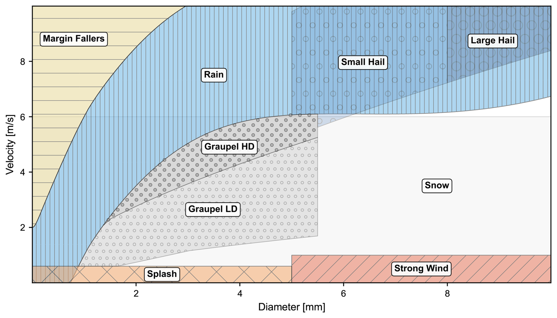
Figure 4 Schematic illustration of particle size–velocity spectrum partitioning, inspired by Friedrich et al. (2013) and derived from theoretical fall velocity–particle size relationships (see Appendix B). The hydrometeor masks are automatically adjusted according to the station altitude.

Graupel is assumed to have diameters between 1 and 5 mm, while hail particles exceed 5 mm. Snow is identified as particles with estimated fall velocities up to 6.5 m s⁻¹. Artefacts such as drop splashing and margin fallers are also explicitly recognized: splashing generates small particles with unrealistically low fall velocities, whereas margin fallers show abnormally high fall velocities relative to their underestimated diameters. Additionally, strong winds (>20 m s⁻¹) combined with intense rainfall can produce large but slow-falling particles (D>5 mm, v<1 m s⁻¹), as reported by Friedrich et al. (2013).

From these masks applied to the raw particle size-velocity spectrum, the HC algorithm computes particle counts, relative fractions, and occupied bins for each hydrometeor type, then applies a set of physically based decision rules to assign a preliminary hydrometeor label. This logic distinguishes drizzle, rain, snow, and other frozen hydrometeors such as graupel, hail, and ice pellets, while also identifying non-hydrometeor particles and artefacts related to drop splashing, margin fallers and strong winds (Friedrich et al., 2013). When temperature data are available, the classification is refined: thresholds near ±5 °C adjust the liquid-solid boundary, improving the separation between drizzle and snow grains (ice crystals and prisms) and between graupel (T>0 °C) and ice pellets or sleet (T<0 °C). In addition to hydrometeor and precipitation-type classification, the HC module also outputs several quality-control flags, along with the total particle count and class-specific counts. All variables produced by the HC module are listed in Table 2.

(Friedrich et al., 2013)

Table 2 Hydrometeor classification, precipitation phase, flags, and particle count variables produced by the disdrodb classification module.

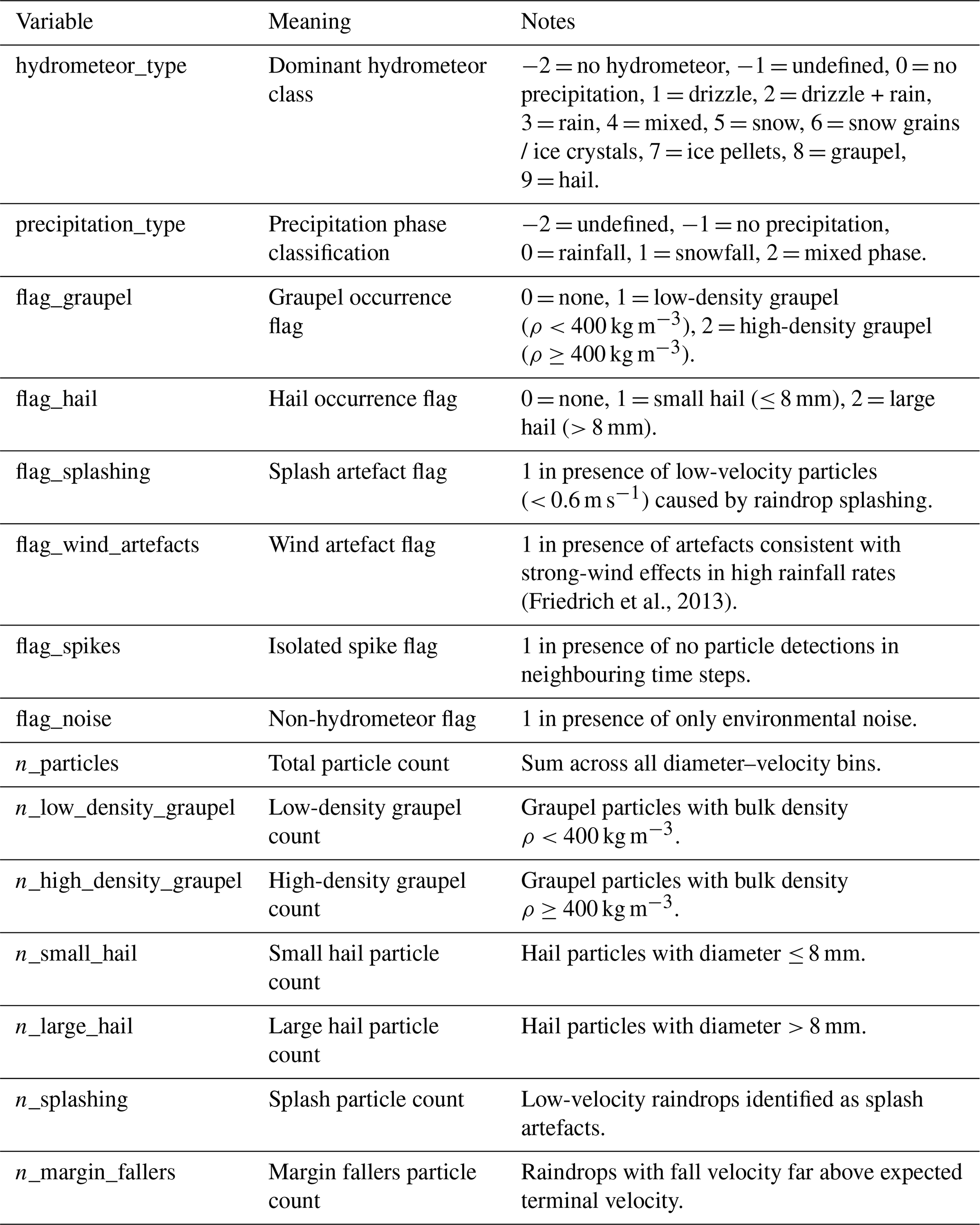
Figure 5 illustrates the time-accumulated raw diameter-velocity particle number spectra n(D,V) for three selected events, each characterized predominantly by a different precipitation type: liquid, mixed, and solid. The temporal evolution of the raw particle number concentration N(D) during these events, together with the precipitation type inferred by the HC module, is presented through quicklook visualizations. The disdrometer station shown in the figure was not used during algorithm development, illustrating the ability of the HC algorithm to generalize to unseen data.

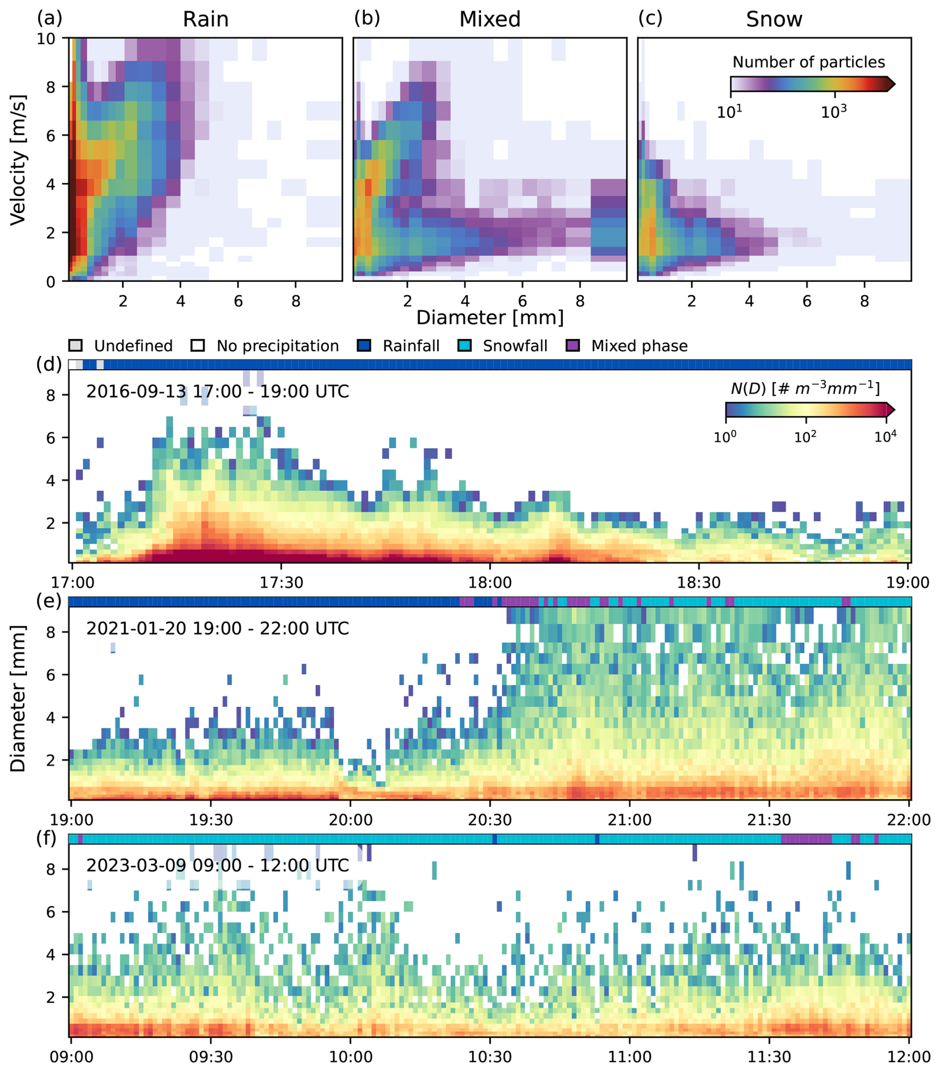
Figure 5 Particle size distributions for liquid, mixed and solid precipitation during three selected events observed by a Thies LPM disdrometer installed at the Whitworth Meteorological Observatory, University of Manchester, United Kingdom. (a–c) Time-accumulated raw diameter-velocity particle number spectra n(D,V) for events predominantly characterized by (a) rain, (b) mixed-phase precipitation, and (c) snow. Colors indicate the total number of detected particles per diameter-velocity bin during the event. (d–f) Temporal evolution of the raw particle number concentration N(D) for the same events. The colored bar at the top of each panel indicates the precipitation type inferred by the HC module. The disdrodb functions plot_spectrum and plot_dsd_quicklook allow easy reproduction of these figures with every DISDRODB product.

To the best of our knowledge, disdrodb provides the first open-source disdrometer-based hydrometeor classification algorithm capable of detailed partitioning of hydrometeor classes and precipitation phases. In contrast to sensor firmware-specific, undisclosed, proprietary algorithms, it accounts for the effect of altitude-dependent air density on particle fall velocity, and applies a transparent, consistent classification scheme across all DISDRODB stations.

Comparisons with weather codes reported by the instrument's internal software show very good agreement. Although the current results are promising, ongoing work aims to further refine the HC module and evaluate its performance against independent ground-based instruments, with particular focus on the identification of frozen particles. Planned developments include extending the classification to generate standard World Meteorological Organization (WMO) SYNOP, METAR/SPECI, and NWS weather codes (WMO, 2019).

6 DISDRODB L2 products

In the L2 processing chains, disdrodb allows users to retrieve integral parameters and polarimetric radar variables from empirical (L2E) or modelled (L2M) particle size distributions. For rainfall, the relevant physical relationships are sufficiently well constrained that its microphysical and bulk properties can be reliably estimated. Raindrops can be reasonably approximated as spheroids of nearly constant density and known size-dependent axis ratio, with fall velocity primarily governed by their equivolume spherical drop diameter. This enables the derivation of drop size distribution (DSD) parameters from the particle sizes measured by disdrometers, as well as the simulation of polarimetric radar observables through T-matrix scattering models under the spheroidal particle assumption.

In contrast, the characterization of snow particles is far more uncertain. Snowflakes exhibit substantial variability in shape, density, and fall behavior, depending on their growth habit (e.g., dendritic, columnar, or aggregate structures) and degree of riming (Locatelli and Hobbs, 1974; Mitchell et al., 1990; Mitchell, 1996; Barthazy and Schefold, 2006; Brandes et al., 2008; Kikuchi et al., 2013; Grazioli et al., 2022; Vázquez-Martín et al., 2021a, b). Converting the horizontally projected particle size measured by disdrometers, which is itself uncertain due to internal air pockets and the different optical properties of ice relative to liquid water, into physically meaningful quantities such as maximum dimension, bulk density, mass, or fall velocity requires strong, case-dependent assumptions (Battaglia et al., 2010). Estimating radar polarimetric signatures of snow and mixed-phase precipitation is equally challenging, as they depend on particle orientation, aspect ratio, internal structure, degree of riming or melting and the air-ice mixture within the scattering volume (Liu, 2008; Hong, 2007; Leinonen et al., 2012; Liao and Meneghini, 2013; Kneifel et al., 2018, 2020; Ori et al., 2021).

Because of these fundamental uncertainties, the current L2 processing chains in disdrodb focus on rainfall, for which particle microphysics and electromagnetic scattering properties are relatively well constrained. However, the software has been designed to facilitate future extensions, toward solid and mixed-phase precipitation quantification, once robust parameterizations and suitable validation datasets become available.

6.1 DISDRODB L2E products

The DISDRODB L2E (empirical) processing chain computes drop size distribution (DSD) integral parameters and simulates polarimetric radar observables using T-matrix scattering calculations. The following paragraphs describe the general workflow, while Appendices C and E detail the computation of DSD bulk (integrated) quantities (see Table 3) and the simulation of polarimetric variables, respectively (see Table 6).

Table 3 Summary of DSD spectral (size-resolved) and bulk (integrated) quantities included in the current version of DISDRODB L2E and L2M products, together with their units and equation references. Users can extend the set of variables by modifying the open-source disdrodb software. Radar variables included in both DISDRODB L2E and L2M products are listed separately in Table 6.

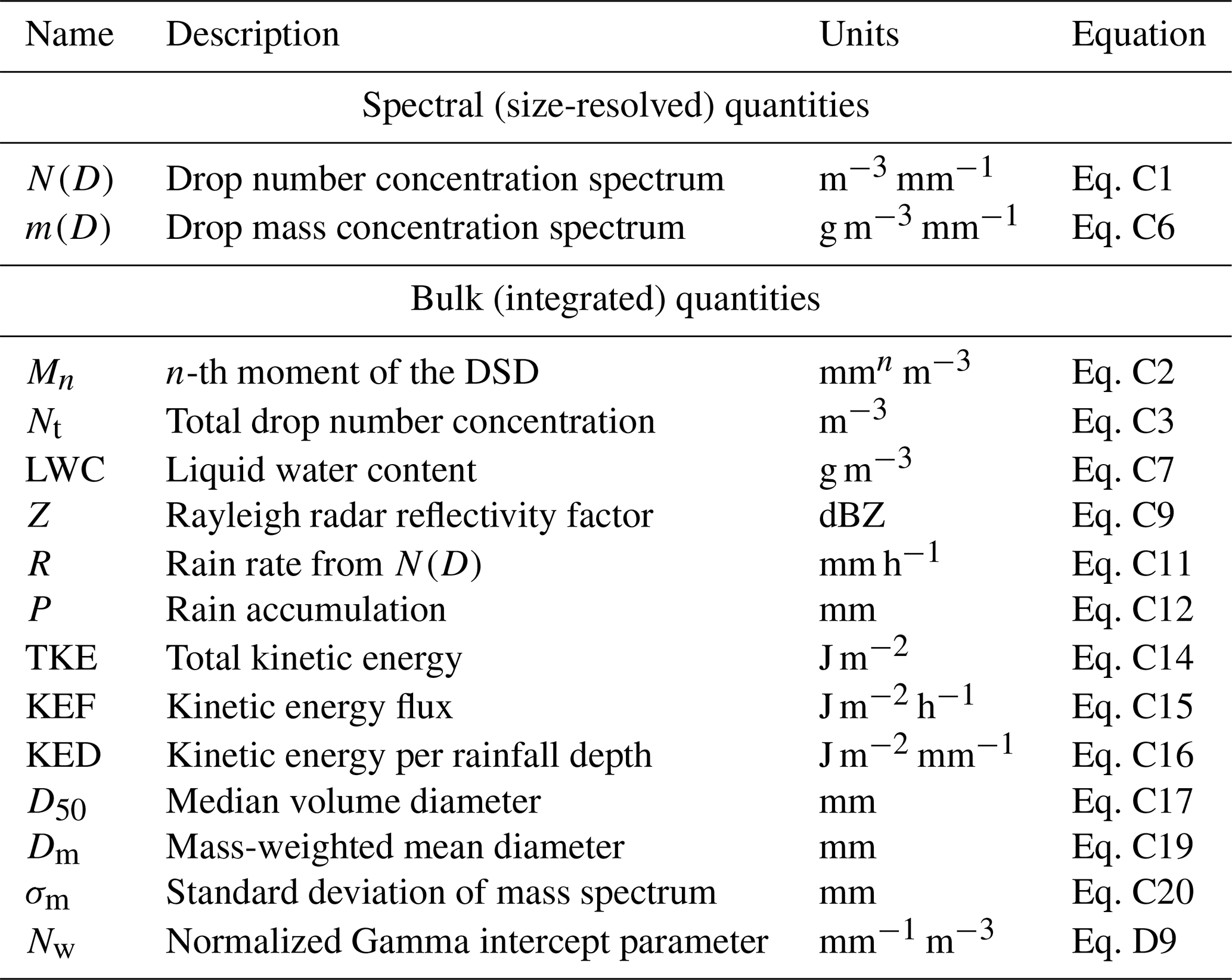
The chain takes as input an L1 dataset containing the raw particle number spectrum and first selects time steps classified as liquid precipitation, based on the precipitation_type variable when available. Then, it filters the two-dimensional spectrum to retain only physically consistent raindrop bins, applying user-defined limits on diameter and fall velocity. By default, drops smaller than 0.25 mm or larger than 10 mm are excluded. Although the smallest bins contribute negligibly to rainfall rate and mass-weighted moments, they can introduce significant noise in lower-order moments such as the total drop number concentration (N_t) (see Eq. C3).

When the full diameter-velocity particle number spectrum n(D,V) is available (i.e., for optical disdrometers other than ODM470), the algorithm filters the spectrum based on the theoretical terminal fall velocity of raindrops, combined with user-defined filtering criteria. Only particles whose measured velocities lie within a specified percentage or absolute tolerance around the expected terminal velocity are retained. This velocity-based filtering step removes spurious detections such as splashing or margin fallers and enforces physical consistency between particle size and velocity. Typical thresholds used in the literature range between V−3 m s⁻¹ and V+4 m s⁻¹, or between 25 %–75 % below/above the theoretical terminal fall velocity (Raupach and Berne, 2015; Friedrich et al., 2013; Jaffrain and Berne, 2011; Tokay et al., 2001). These thresholds must consider sensor uncertainty and the natural occurrence of drops falling at sub- or super-terminal velocities due to microphysical processes or turbulence (Montero‐Martínez et al., 2009; Larsen et al., 2014; Montero‐Martínez and García‐García, 2016). Under strong horizontal winds, changes in the orientation of large raindrops modify the aerodynamic drag acting on them, thereby altering their terminal fall speed. Preliminary analyses of DISDRODB stations also show that instruments mounted on roofs report, on average, lower fall velocities than expected and broader velocity distributions, likely caused by turbulence and vertical wind. To avoid inadvertently removing valid particles and underestimating parameters such as rain rate, thresholds must therefore be chosen with care.

For optical disdrometers that report the full diameter-velocity particle number spectrum n(D,V), the drop number concentration N(D) is computed in two ways: (1) using the measured fall velocity and (2) using the theoretical terminal fall velocity estimated from the specified drop fall-velocity model. For impact disdrometers and ODM470, which record only the one-dimensional spectrum n(D), N(D) is estimated solely from the theoretical terminal fall velocity.

From N(D), the L2E processing chain derives a comprehensive set of DSD bulk (integrated) quantities, drop-size and bin statistics, and polarimetric radar variables simulated through T-matrix scattering (see Sect. 6.3). When n(D,V) is available, additional quantities such as kinetic energy variables and rainfall rate are directly computed from the filtered spectrum n(D,V) using the instrument-measured fall velocity. This allows for direct comparison between quantities derived from N(D) and those calculated from the measured spectrum. The processing chain is fully customizable, and optional thresholds can be applied to exclude time steps with insufficient data quality – such as those containing too few drops, too few populated bins, or rain rates below a configurable minimum (see Fig. 3).

All variables generated by the L2E processing chain are summarized in Table 3; the simulated radar polarimetric variables are presented separately in Table 6. Together, these variables provide the foundation for a comprehensive analysis of statistical relationships among DSD bulk quantities and radar observables, supporting the development and evaluation of radar retrieval algorithms and microphysical parameterization schemes. Figure 6 illustrates the relationships among key DSD parameters, while Fig. 7 presents the power-law dependencies between rainfall rate and simulated radar variables. These types of diagnostic figures are automatically generated by disdrodb as part of the station summary product.

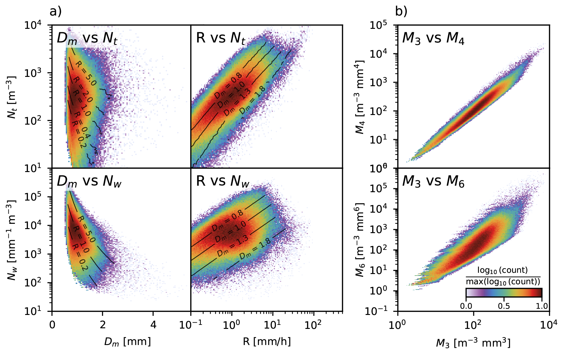
Figure 6 Two-dimensional histograms illustrating the relationships among DSD bulk quantities derived from 15 years of measurements collected by a Thies LPM disdrometer installed at the Whitworth Meteorological Observatory, Manchester University, United Kingdom. Colors represent the normalized logarithmic frequency of occurrence. (a) Relationships among D_m, N_t, N_w and R. Black contour lines indicate median iso-R values in the left column and median iso-D_m values in the right column. A decreasing trend of N_w with increasing D_m is observed, while R generally increases with both D_m and N_t. No clear relationship is evident between D_m and N_t, nor between N_w and R. (b) Relationships between the third moment M₃ and higher-order moments M₄ (top) and M₆ (bottom), commonly used in double-moment DSD normalization approaches (see Appendix D). Similar diagnostic plots exploring additional DSD bulk relationships are automatically generated by disdrodb as part of the station summary figures.

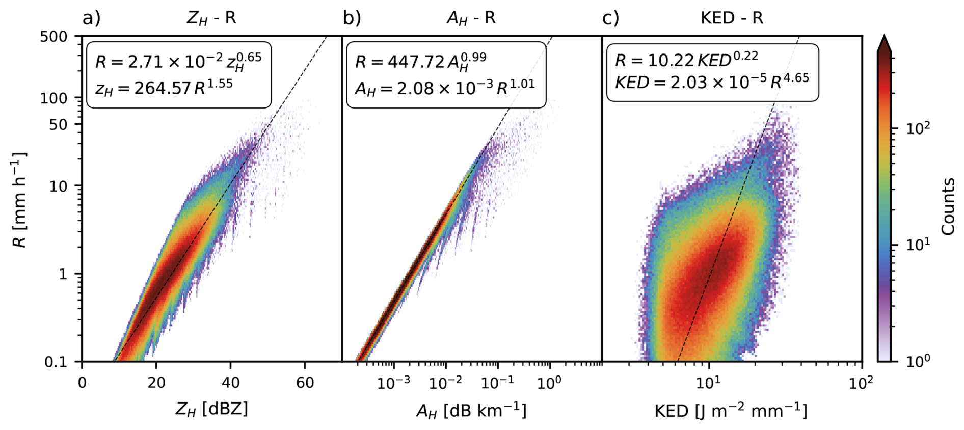
Figure 7 Two-dimensional histograms illustrating power-law relationships between rainfall rate R and selected radar and microphysical variables derived from 15 years of disdrometer measurements at Whitworth Meteorological Observatory. Colors indicate the frequency of occurrence (counts), while black dashed lines represent the fitted power-law relationships shown in each panel. Power-law relationships are fitted by default using the robust RANSAC algorithm (Fischler and Bolles, 1981) applied to the median values within each bin; weighted nonlinear least squares is also available as an alternative. Inverse power-law relationships are obtained by algebraic inversion of the fitted models. (a) C-band horizontal reflectivity factor Z_{H, C} versus R. The z_H in the power-law expressions denotes reflectivity in linear units, and the regression is performed on z_H. (b) C-band horizontal specific attenuation A_{H, C} versus R. (c) Kinetic energy density (KED) versus R. Similar diagnostic plots, including additional radar variables at multiple frequency bands and kinetic energy relationships, are automatically generated by disdrodb as part of the station summary figures.

6.2 DISDRODB L2M products

The DISDRODB L2M (modelling) processing chain allows users to fit parametric DSD models to the observed empirical DSD. It then computes integral DSD parameters and polarimetric radar variables from the modelled distribution. The following paragraphs describe the general workflow and applications of L2M products. Appendix D provides the mathematical definition of the parametric DSD models.

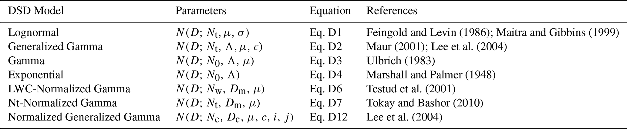
The L2M chain takes as input an L2E dataset containing the observed drop number concentration N(D). For each time step, the software estimates the parameters of the selected statistical models. The software implements six widely used parametric DSD models: lognormal, exponential, gamma, normalized gamma, generalized gamma, and normalized generalized gamma. Table 4 summarizes these models and their parameters.

Feingold and Levin (1986); Maitra and Gibbins (1999)Maur (2001); Lee et al. (2004)Ulbrich (1983)Marshall and Palmer (1948)Testud et al. (2001)Tokay and Bashor (2010)Lee et al. (2004)

Table 4 Summary of DSD parametric models implemented in disdrodb.

Several fitting methods are available, from brute-force grid search (GS) to unconstrained or constrained maximum likelihood (ML) and the method of moments (MOM). The models to be fitted are defined in the DISDRODB product configuration files, and users can adjust the optimization settings, as well as specify optional thresholds restricting the time steps on which to fit the statistical models. For microphysical DSD studies, we recommend estimating the model parameters by minimizing errors in N(D). For the development or validation of radar and satellite retrievals, the fitting procedure should take care to also minimize errors in integral parameters such as LWC, R or Z. The GS routine provides the flexibility to minimize multiple objectives through a weighted loss function and custom variable transformations.

An evaluation of fitting procedures (not shown here) indicates that the method of moments produces inaccurate parameters even when the observed DSD follows the assumed parametric model functional form. Maximum-likelihood estimators may also converge to biased parameters because of local minima in the loss function. Therefore, although slightly more computationally demanding, we recommend estimating model parameters using a grid search that minimizes the sum of squared errors of N(D) as the primary objective, optionally complemented by the mean absolute or squared error of a bulk DSD quantity such as LWC or Z.

Once the model parameters are estimated, integral DSD parameters and polarimetric radar variables are computed from the modelled drop number concentration N_MODEL(D;θ). A set of goodness-of-fit (GOF) statistics is computed to assess the accuracy of each fitted model; the metrics are summarized in Table 5. Users may also compute additional error metrics, for example by comparing rain rate or radar variables derived from the L2E product with those obtained from the modelled N_MODEL(D;θ) in the L2M product.

Table 5 Goodness-of-fit metrics computed between observed and L2M predicted DSDs. For a diameter bin D_i with width ΔD_i, the probability mass is defined as $p\left(D_i\right)={\displaystyle \frac{N\left(D_i\right)\mathrm{\Delta }{D}_i}{N_{\mathrm{t}}}}$. The cumulative distribution function is defined as $F\left(D_i\right)={\sum }_{i\le n}p\left(D_i\right)$.

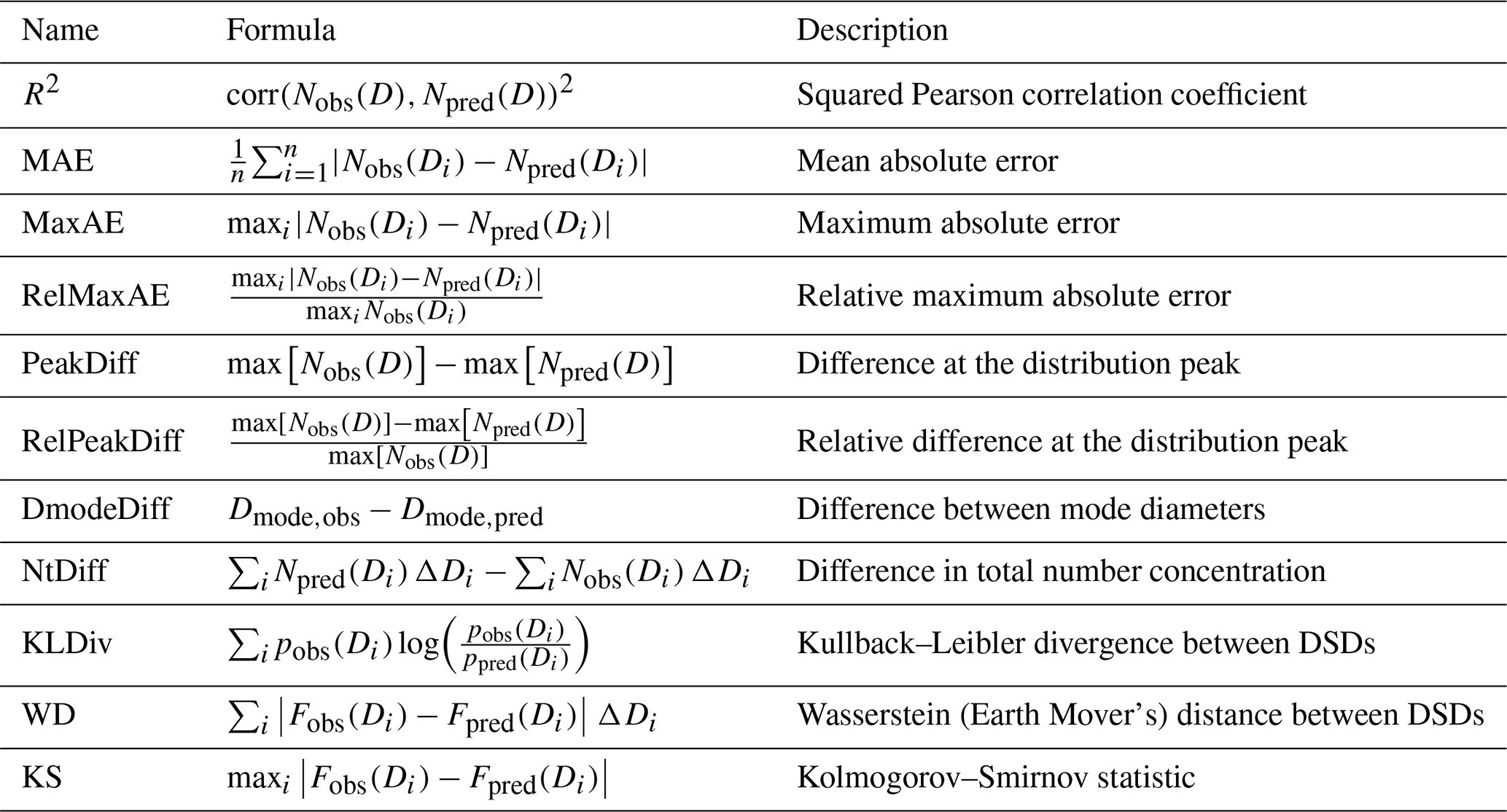
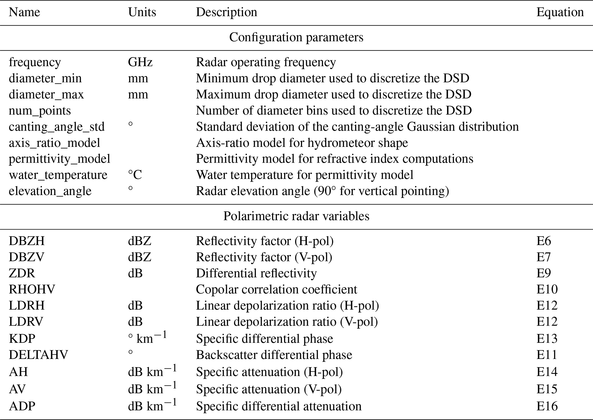
Table 6 List of the T-matrix configuration parameters and the radar variables calculated for both DISDRODB L2E and L2M products.

Among the GOF metrics, the Kullback-Leibler divergence (KLDiv) is commonly used to quantify how much a parametric DSD model differs from the observations and to identify the statistical model that best fits the observed distributions (Adirosi et al., 2016; Cugerone and Michele, 2015; Gatidis et al., 2020). Figure 8a evaluates the adequacy of the DSD parametric models implemented in disdrodb for representing observed DSDs at 1 min temporal resolution. Models with a larger number of free parameters (see Table 4) provide increased structural flexibility and are thus better suited to capture the shape variability of the observed DSDs, but they also increase the risk of overfitting.

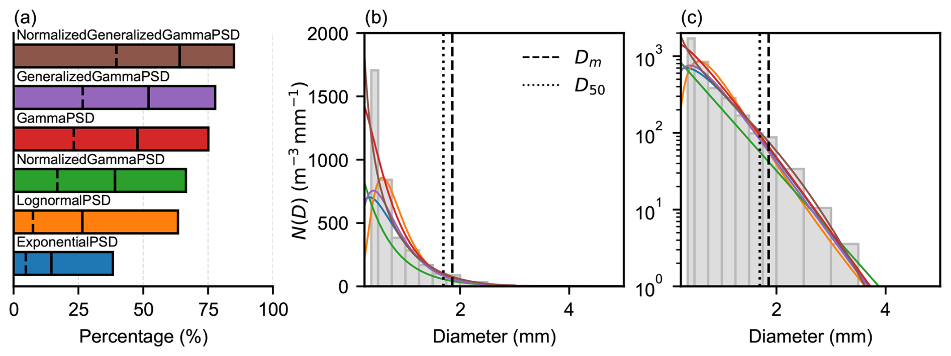
Figure 8 Illustration of the adequacy of DSD parametric models in reproducing DSDs observed during 15 years of disdrometer measurements at the Whitworth Meteorological Observatory. (a) Percentage of total observations well fitted by each DSD parametric model. Model parameters are estimated using a grid-search procedure minimizing the sum of squared errors (SSE) of log ₁₀(N(D)) together with the absolute error in Z. Model performance is evaluated using the Kullback-Leibler divergence (KLDiv); vertical markers indicate the percentage of cases with KLDiv below 0.025, 0.05, and 0.1. (b–c) Example of an observed DSD at a given time step fitted with the various parametric models, shown on (b) linear and (c) logarithmic y-axis scales. Vertical lines indicate the mass-weighted mean diameter (D_m, dashed) and the median volume diameter (D₅₀, dotted). Drops with diameters larger than D₅₀ contribute half of the liquid water content within the sampled air volume.

However, for real applications, the number of free parameters of N_MODEL(D;θ) is constrained by the amount of independent information available. Dual-frequency and polarimetric radar DSD retrieval algorithms therefore typically adopt an N_MODEL(D;θ) with two free parameters (Zhang et al., 2001; Liao et al., 2014; Gatidis et al., 2022; Lee et al., 2023; Ladino-Rincon et al., 2025).

The double-moment normalization framework (Lee et al., 2004), combined with long-term DSD observations, enables the identification and fitting of a parametric model, assumed to be invariant in space and time, that expresses the DSD as a function of only two moments (see Appendix D3). These moments and their corresponding general characteristic diameter (D_c; Eq. D10) and intercept (N_c; Eq. D11) can then be retrieved from the radar observables either through empirical relationships or machine learning algorithms, and subsequently used to reconstruct the DSD (Raupach and Berne, 2017; Raupach et al., 2019; Shin et al., 2024). Figure 9 illustrates the observed double-moment normalized DSDs, corresponding fitted normalized parametric models, and the relationships between the D_c and N_c parameters and radar reflectivities at Ku and Ka bands.

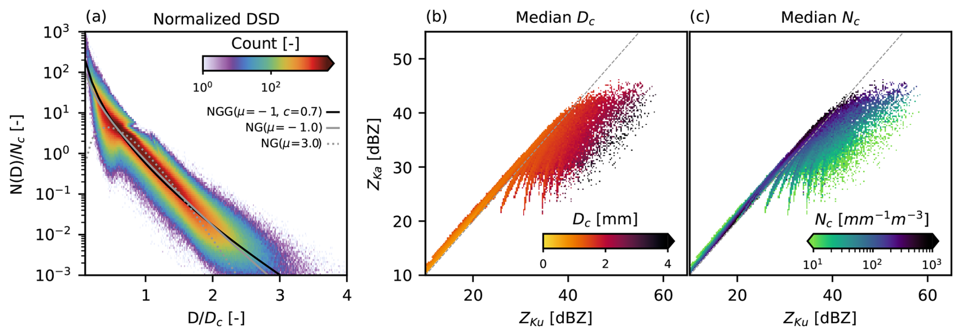
Figure 9 Double-moment normalization analysis and radar relationships derived from 15 years of disdrometer measurements at Whitworth Meteorological Observatory. (a) Observed double-moment normalized DSDs expressed as $N\left(D\right)/N_{\mathrm{c}}$ versus $D/D_{\mathrm{c}}$, using moments i=3 and j=4. Colors indicate the frequency of occurrence (counts). The solid gray and black curves show fitted normalized gamma (NG) and normalized generalized gamma (NGG) models, while the gray dashed line shows the NG parametric model with μ=3 currently adopted in GPM DPR retrievals. (b) Relationship between Ku-band reflectivity Z_Ku and Ka-band reflectivity Z_Ka, with color shading indicating the observed median general characteristic diameter D_c. D_c grows monotonically with increasing reflectivities. (c) Relationship between Ku-band reflectivity Z_Ku and Ka-band reflectivity Z_Ka, with color shading indicating the observed median general characteristic intercept parameter N_c. Retrieval of N_c becomes particularly challenging for Z_Ku < 30 dBZ, where large variations in N_c produce only small changes in Z_Ka. This region is associated with negative dual-frequency ratio (DFR) values and corresponds to the area above the 1:1 dashed gray line.

6.3 Radar simulations with T-matrix

Rainfall polarimetric radar variables in DISDRODB are simulated using electromagnetic scattering calculations based on the T-matrix method, which numerically solves Maxwell's equations for scattering by non-spherical raindrops (Mishchenko et al., 1996). The simulations can be based either on the empirical drop number concentration available in the L2E products or on the parametric DSD models estimated in the L2M products. The disdrodb wrapper around PyTMatrix (Leinonen, 2014) enables vectorized and parallelized computations, provides flexible configuration of the radar settings and microphysical assumptions, and manages caching of the corresponding scatterer objects to avoid redundant T-matrix simulations. It also allows users to easily explore the sensitivity of the simulated radar variables to different parameter choices (Fig. E2). Table 6 summarizes the user-configurable parameters and the simulated radar variables, while Appendix E provides additional mathematical details on the T-matrix method and the definitions of the simulated radar quantities.

Radar variables are computed in two steps. First, the scattering amplitude matrices obtained from T-matrix calculations are evaluated in backward-scattering geometry, which corresponds to the radar-receiving direction and is required to compute horizontal and vertical polarization reflectivities (DBZH and DBZV), as well as polarimetric variables such as differential reflectivity (ZDR), linear depolarization ratios (LDR), backscatter differential phase (DELTAHV) and the co-polar correlation coefficients (RHOHV). Second, the same scattering quantities are evaluated in forward-scattering geometry, which governs how the radar signal propagates through the medium and is therefore used to compute the propagation-related variables such as the specific differential phase (KDP), specific attenuation at horizontal and vertical polarizations (AH and AV), and the differential attenuation (ADP).

The radar frequency and elevation angle determine the scattering regime and the viewing geometry used in the T-matrix calculations. The minimum and maximum drop diameter (diameter_min and diameter_max), along with the number of diameter bins (num_points), control the numerical discretization of the DSD and particles sizes used in the T-matrix calculations. The chosen axis-ratio model specifies how drop oblateness increases with diameter, while the canting-angle Gaussian distribution sets the spread of drop orientations around the vertical; this orientation variability directly affects polarimetric variables such as ZDR, LDR, and RHOHV by modulating the effective asymmetry and depolarization of the scattering (Fig. E2b). The water permittivity model and water temperature, together with the radar frequency, determine the complex refractive index of water and the corresponding radar dielectric factor (Fig. E2c). disdrodb includes the formulations of Liebe et al. (1991), Ellison (2007) and Turner et al. (2016). These dielectric properties, which are significantly affected by the temperature of the hydrometeors, primarily influence the magnitude of scattering and absorption and therefore directly affect reflectivity and attenuation-related variables (DBZH, DBZV, ZDR, AH, AV, ADP) as well as phase-based quantities such as KDP and PHIDP.

The modular design of disdrodb further allows the integration of alternative electromagnetic scattering models (e.g., Mie theory, or scattering databases based on Discrete Dipole Approximation (DDA) or Rayleigh-Gans approximations), enabling radar-variable simulations for a broader range of hydrometeor types. The simulation of Doppler spectra is not currently implemented but may be incorporated in future developments. Within the current implementation, the disdrodb pytmatrix wrapper allows users to easily explore how simulation settings influence radar observables and assess their sensitivity to different parameters. As an example of the sensitivity of radar observables to simulation settings, Fig. E2 illustrates the impact of water temperature, canting angle spread, and radar viewing geometry on DBZH and ZDR at C band.

7 Conclusions

This article presents DISDRODB and the open-source Python package disdrodb, a community framework designed to improve the accessibility, standardization, and reproducibility of disdrometer data analysis. The work addresses three persistent limitations in disdrometer-based research: the scarcity of easily usable public datasets, the heterogeneity of raw data formats and instrument-specific outputs, and the lack of transparent, maintainable processing workflows that can be consistently applied across stations and sensor types.

DISDRODB combines a centralized metadata archive with a decentralized data-sharing model, allowing institutions to retain control and authorship of their raw data while making datasets globally discoverable and straightforward to access and download through a common interface. This architecture lowers the barrier to contribution, respects institutional data-governance constraints, and provides a scalable foundation for long-term community growth.

The disdrodb software implements a modular three-level processing chain that converts heterogeneous raw disdrometer measurements into harmonized, analysis-ready products. The L0 processing chain standardizes raw records into netCDF4 files. The L1 processing chain performs temporal resampling, quality control, and hydrometeor/precipitation-type classification based on raw size–velocity spectra. In contrast to proprietary firmware-based algorithms, the hydrometeor-classification approach implemented in disdrodb is transparent, altitude-aware, and reproducible; it can be applied consistently across stations and sensor types, and can be inspected, tested, and improved by the community. The L2 processing chains derive PSD integral parameters, fit parametric PSD models, and simulate radar variables through T-matrix scattering calculations, which substantially expands the value of disdrometer observations for radar and remote-sensing applications. Summary figures and tables can be automatically generated after L2 processing to support rapid exploratory analysis and station-level problem identification.

By providing a transparent and reproducible workflow from raw data to derived products, the software removes much of the time researchers currently spend on data wrangling, format harmonization, and re-implementing instrument-specific processing steps, allowing them to focus on scientific analysis and on identifying methodological improvements. The software also supports flexible execution modes (single-process, parallel, and distributed), enabling efficient processing of large numbers of stations and long time series, on both small computing environments and large clusters. Finally, its modular architecture facilitates future extensions, including ingestion of new sensors, processing methods, quality-control procedures, and derived products contributed by the community.

At the same time, DISDRODB does not remove the intrinsic limitations of disdrometer measurements. Instrument-specific biases, wind effects, sampling uncertainty, proprietary undisclosed on-board particle filtering, and uncertainties in the characterization of frozen and mixed-phase hydrometeors remain important challenges. However, DISDRODB provides a common framework to document, compare, and analyze them systematically across sensors and sites. This is an essential step toward improved disdrometer intercomparison, uncertainty characterization, and evidence-based instrument development.

The current L2 processing chains focus on rainfall, where particle microphysics and electromagnetic scattering assumptions are comparatively well constrained. Future developments could target improved treatment of frozen and mixed-phase precipitation, further refinement and validation of the hydrometeor-classification module against independent observations, and expansion of derived products and radar retrieval-oriented tools. The software design also supports the integration of additional sensors, processing methods, and scattering models as the field evolves.

We look forward to the participation of new institutions in the DISDRODB initiative, both through the contribution of new disdrometer stations and through community-driven development of the open-source software. The progressive consolidation of a public, global, and homogeneous database of disdrometer measurements will advance our understanding of rainfall characteristics and variability across climates and regions, and will foster new applications in precipitation microphysics, remote sensing, and related fields.

Appendix A: Drop axis ratio models

The deformation of falling raindrops from a perfect sphere into an oblate shape under aerodynamic forces is commonly characterized by the axis ratio $a_{\mathrm{r}}=\frac{B}{A}$, where A and B denote the full major (horizontal) and minor (vertical) axes (Szakáll et al., 2010; Beard et al., 2010). The drop size is expressed through the equivolumetric spherical diameter D (also commonly denoted D_eq), defined as the diameter of a sphere having the same volume as the oblate spheroid. The spheroid volume is defined as $V=\frac{\mathrm{4}}{\mathrm{3}}\mathit{\pi }{\left(\frac{A}{\mathrm{2}}\right)}^{\mathrm{2}}\left(\frac{B}{\mathrm{2}}\right)=\frac{\mathrm{4}}{\mathrm{3}}\mathit{\pi }{\left(\frac{D}{\mathrm{2}}\right)}^{\mathrm{3}}$. From this relationship, it follows that $D=A{a}_{\mathrm{r}}^{\mathrm{1}/\mathrm{3}}=B{a}_{\mathrm{r}}^{-\mathrm{2}/\mathrm{3}}$.

Values of a_r=1 correspond to spherical drops, a_r<1 to oblate drops, and a_r>1 to prolate drops. This parameterization enables the use of an equivalent oblate spheroid in radar scattering simulations, where drop nonsphericity strongly influences electromagnetic scattering and wave propagation, particularly the differential reflectivity (ZDR) and the specific differential phase (KDP).

Table A1 summarizes the axis-ratio parameterizations implemented in disdrodb, and Fig. A1 illustrates drop axis-ratio values as a function of the equivolumetric spherical diameter D. For PARSIVEL and PARSIVEL2 disdrometers, which report D after assuming the PARSIVEL axis-ratio model a_r, P (Battaglia et al., 2010), the horizontal drop axis A can be reconstructed as $A=\frac{D}{a_{\mathrm{r},\mathrm{P}}(D{)}^{\mathrm{1}/\mathrm{3}}}$. Given the measured horizontal drop size A and an assumed axis-ratio model, the corresponding equivolumetric spherical diameter D is obtained by solving $D=\arg {min}_{D^{\prime }>\mathrm{0}}\left|A{a}_{\mathrm{r}}(D^{\prime }{)}^{\mathrm{1}/\mathrm{3}}-D^{\prime }\right|=\arg {min}_{D^{\prime }>\mathrm{0}}\left|\frac{D^{\prime }}{a_{\mathrm{r}}(D^{\prime }{)}^{\mathrm{1}/\mathrm{3}}}-A\right|$.

Sensitivity analyses indicate that using any of the available axis-ratio models results in relative rainfall-rate differences of less than 2 %. However, the choice of axis-ratio model can have a pronounced effect on polarimetric radar variables such as differential reflectivity (see Fig. E2b).

Because the internal processing algorithms of most disdrometers included in disdrodb are not fully documented, with the partial exception of PARSIVEL sensors, disdrodb currently assumes that the measured and reported particle size corresponds to the equivolumetric spherical drop diameter D, rather than to the horizontal particle size A. If this assumption is violated, all bulk DSD quantities and simulated radar variables tend to be systematically overestimated. This arises from a size overestimation for larger drops (since A>D) caused by their increasing departure from sphericity (see Fig. A1). A bias analysis showed that the resulting overestimation leads to a positive bias in rainfall rate that grows with intensity, exceeding 15  % for rates above 50 mm h⁻¹.

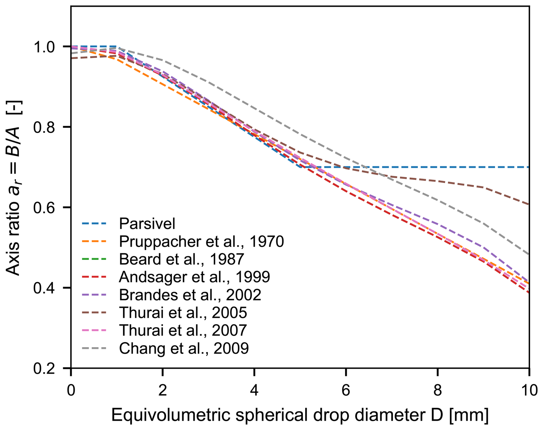
Figure A1 Comparison of the drop axis ratio as a function of drop diameter for parameterizations implemented in disdrodb.

Pruppacher and Pitter (1971)Beard and Chuang (1987)Andsager et al. (1999)Brandes et al. (2002)Thurai and Bringi (2005)Thurai et al. (2007)Chang et al. (2009)Battaglia et al. (2010)

Table A1 Summary of axis–ratio relationships for raindrops. Equivolumetric spherical drop diameter (D) is in mm.

Appendix B: Terminal fall-velocity models

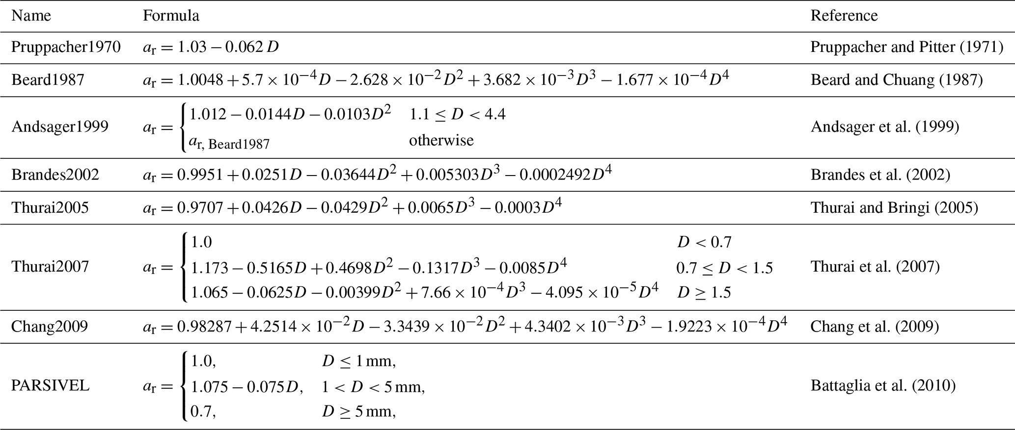
The terminal fall velocity is defined as the velocity attained by a particle falling through still air when the drag and buoyancy forces balance gravity. In this appendix we describe rainfall, graupel, and hail fall-velocity models implemented in the disdrodb software. The modular structure of the software also allows new models to be incorporated readily as improved or revised parameterizations become available.

B1 Raindrop terminal fall velocity

Raindrop fall velocities can be estimated using empirical relationships derived from field and laboratory measurements. Table B1 summarizes the relationships included in disdrodb, while Fig. B1 illustrates the dependence of raindrop terminal fall velocity on drop diameter and air density. Terminal velocity increases primarily with drop diameter, but tends to level off at diameters near 5 mm. For a given diameter, it increases with decreasing air density, and is therefore greater at higher altitudes and under warmer atmospheric conditions.

To account for changes in air density with altitude, disdrodb applies the correction proposed by Beard (1985):

$$\begin{array}{}\text{(B1)}& v_{\mathrm{h}}\left(D\right)=v_{\mathrm{0}}\left(D\right){\left({\displaystyle \frac{{\mathit{\rho }}_{\mathrm{0}}}{{\mathit{\rho }}_{\mathrm{h}}}}\right)}^{(\mathrm{0.375}+\mathrm{0.025}D)}\end{array}$$

where D is the drop diameter in millimeters, v₀(D) is the terminal fall velocity at sea-level pressure, and ρ₀ and ρ_h are the air densities at sea level and at height h, respectively. ρ₀ is set to 1.225 kg m⁻³ assuming the International Standard Atmosphere. The air density ρ_h is computed following Brutsaert (1982):

$$\begin{array}{}\text{(B2)}& {\mathit{\rho }}_{\mathrm{h}}={\displaystyle \frac{p}{R_{\mathrm{d}}T}}\left(\mathrm{1}-\mathrm{0.378}{\displaystyle \frac{e}{p}}\right)\end{array}$$

where T is the air temperature (K), p is the air pressure (Pa), e is the actual vapor pressure (Pa), and R_d is the gas constant for dry air with a default value of 287.04 J kg⁻¹ K⁻¹. The actual vapor pressure is calculated as $e=\mathrm{RH}\times e_{\mathrm{sat}}\left(T\right)$, where RH is the relative humidity (0–1) and e_sat(T) is the saturation vapor pressure (in Pascals) at temperature T, obtained using the formulation of Flatau et al. (1992).

Beard terminal fall-velocity model

The model of Beard (1976) provides a physically based description of raindrop terminal fall velocity by accounting for the effects of drop shape, drag, and air properties across a wide range of drop sizes. The terminal fall velocity is expressed in terms of the Reynolds number by rearranging its definition:

$$\begin{array}{}\text{(B3)}& v\left(D\right)={\displaystyle \frac{{\mathit{\eta }}_{\mathrm{a}}\mathrm{Re}\left(D\right)}{{\mathit{\rho }}_{\mathrm{a}}D}}\end{array}$$

where η_a is the dynamic viscosity of air (kg m⁻¹ s⁻¹), ρ_a is the air density (kg m⁻³), and Re(D) is the Reynolds number of the drop.

The Reynolds number is defined piecewise, with separate formulations for small and large drops:

$$\begin{array}{}\text{(B4)}& \mathrm{Re}\left(D\right)=\left\{\begin{array}{ll}{\mathrm{Re}}_{\mathrm{small}}\left(D\right),& D<\mathrm{1.07}\mathrm{mm}\\ {\mathrm{Re}}_{\mathrm{large}}\left(D\right),& D\ge \mathrm{1.07}\mathrm{mm}\end{array}\right.\end{array}$$

For small drops (D<1.07 mm), the Davies number is computed as $\mathrm{Da}=\frac{\mathrm{4}{\mathit{\rho }}_{\mathrm{a}}({\mathit{\rho }}_{\mathrm{w}}-{\mathit{\rho }}_{\mathrm{a}})g{D}^{\mathrm{3}}}{\mathrm{3}{\mathit{\eta }}_{\mathrm{a}}^{\mathrm{2}}}$, where ρ_w is the water density (kg m⁻³) and g is the gravitational acceleration (m s⁻²). The corresponding Reynolds number is obtained from an exponential of a sixth-order polynomial with x=ln (Da):

$$\begin{array}{}\text{(B5)}& {\mathrm{Re}}_{\mathrm{small}}\left(D\right)=\exp \left(\sum _{i=\mathrm{0}}^{\mathrm{6}}{b}_i{x}^i\right)\end{array}$$

For large drops (D≥1.07 mm), the Bond number $\mathrm{Bo}=\frac{\mathrm{4}({\mathit{\rho }}_{\mathrm{w}}-{\mathit{\rho }}_{\mathrm{a}})g{D}^{\mathrm{2}}}{\mathrm{3}\mathit{\sigma }}$ and the property number $P=\frac{{\mathit{\sigma }}^{\mathrm{3}}{\mathit{\rho }}_{\mathrm{a}}^{\mathrm{2}}}{{\mathit{\eta }}_{\mathrm{a}}^{\mathrm{4}}({\mathit{\rho }}_{\mathrm{w}}-{\mathit{\rho }}_{\mathrm{a}})g}$ are first computed. The surface tension of pure water σ (N m⁻¹) is derived following the parameterization of Pruppacher and Klett (1978):

$$\begin{array}{}\text{(B6)}& \mathit{\sigma }\left(T\right)=\mathrm{0.0761}-\mathrm{0.000155}T\mathrm{with}T\mathrm{in}\mathit{°}\mathrm{C}\end{array}$$

With $x=\ln \left(\mathrm{Bo}\right)+\frac{\ln \left(P\right)}{\mathrm{6}}$, the Reynolds number for large drops is then estimated as an exponential of a fifth-order polynomial:

$$\begin{array}{}\text{(B7)}& {\mathrm{Re}}_{\mathrm{large}}\left(D\right)=\exp \left({\displaystyle \frac{\ln \left(P\right)}{\mathrm{6}}}+\sum _{i=\mathrm{0}}^{\mathrm{5}}{c}_i{x}^i\right)\end{array}$$

The dynamic viscosity of air, required in the above expressions, is computed using the formulation of Beard (1976):

$$\begin{array}{}\text{(B8)}& \begin{array}{rl}{\mathit{\eta }}_{\mathrm{a}}\left(T\right)& =\left\{\begin{array}{ll}{\displaystyle \frac{\mathrm{1.721}+\mathrm{0.00487}T}{{\mathrm{10}}^{\mathrm{5}}}},& T>\mathrm{0},\\ {\displaystyle \frac{\mathrm{1.718}+\mathrm{0.0049}T-\mathrm{0.000012}{T}^{\mathrm{2}}}{{\mathrm{10}}^{\mathrm{5}}}},& T\le \mathrm{0},\end{array}\right.\\ & \text{with}T\mathrm{in}\mathit{°}\mathrm{C}.\end{array}\end{array}$$

The coefficients used in the above polynomial expressions are listed in Table B2.

Atlas et al. (1973)Beard (1976)Uplinger (1981)Lhermitte (1988)Brandes et al. (2002)van Dijk et al. (2002)Locatelli and Hobbs (1974)Locatelli and Hobbs (1974)Locatelli and Hobbs (1974)Heymsfield et al. (2014)Lee et al. (2015)Heymsfield et al. (2018, 2020)Laurie (1960)Knight (1983)Knight (1983)Heymsfield et al. (2014)Heymsfield et al. (2018, 2020)Fehlmann et al. (2020)

Table B1 Summary of fall-velocity models for rain, graupel, and hail implemented in disdrodb. Diameter D in mm; for rain, D denotes the equivolume diameter, whereas for graupel and hail, D refers to the maximum particle size.

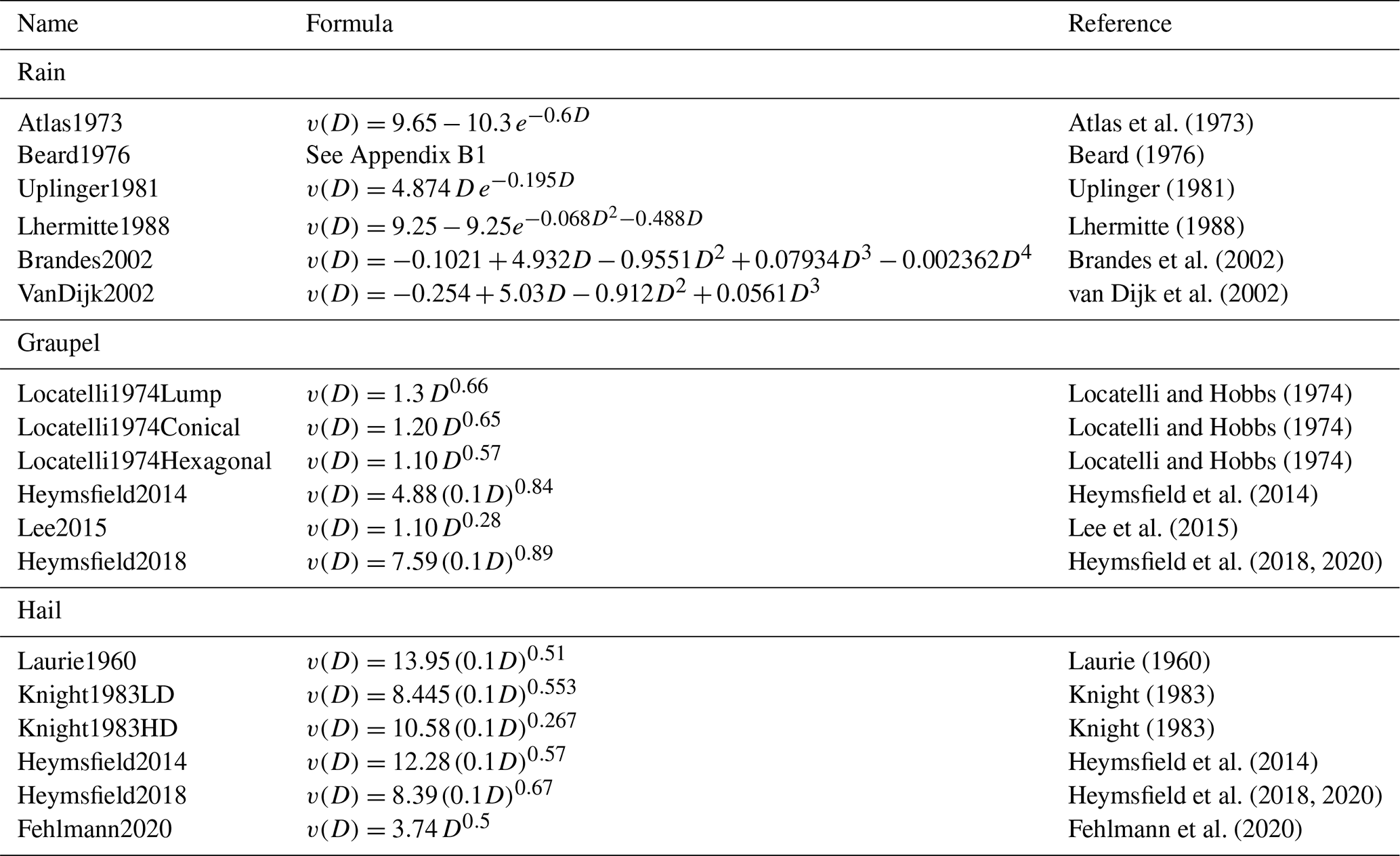
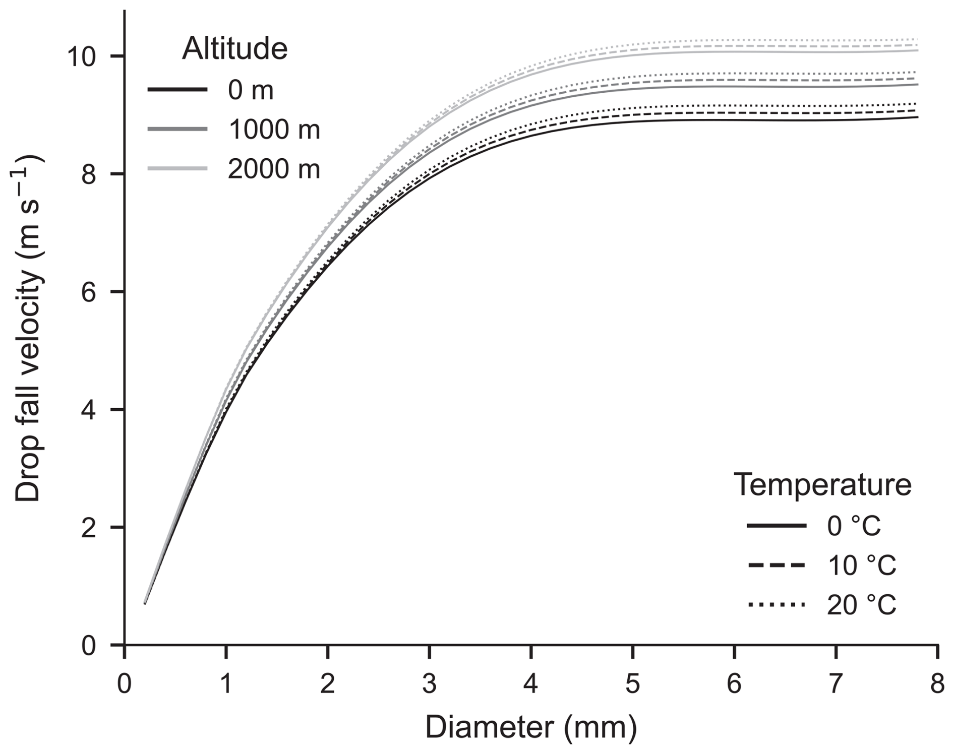
Figure B1 Raindrop fall velocity as a function of drop diameter, altitude, and temperature estimated using the Beard terminal fall-velocity model.

Table B2 Polynomial coefficients for the Reynolds number parameterizations of Beard (1976). Coefficients b_i and c_i apply to small drops (D<1.07 mm) and large drops (D≥1.07 mm), respectively.

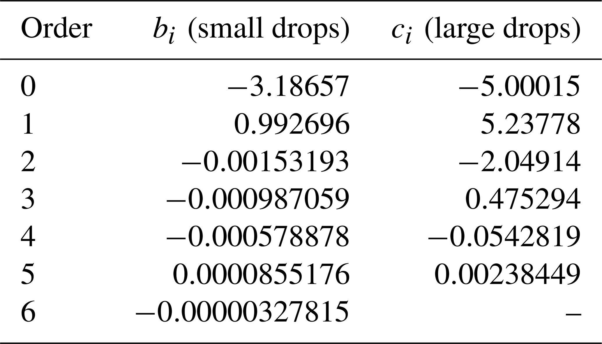
B2 Graupel terminal fall-velocity models

Graupel fall velocities can be estimated using empirical relationships derived from field and laboratory measurements. Table B1 summarizes the graupel parameterizations included in disdrodb. To account for the decrease in air density with altitude, disdrodb applies the correction proposed by Heymsfield and Wright (2014):

$$\begin{array}{}\text{(B9)}& v_{\mathrm{h}}\left(D\right)=v_{\mathrm{0}}\left(D\right){\left({\displaystyle \frac{p_{\mathrm{0}}}{p_{\mathrm{h}}}}\right)}^{\mathrm{0.545}}\end{array}$$

where D is the particle maximum diameter in millimeters, v₀(D) is the terminal fall velocity at sea-level pressure, and p₀ and p_h are the air pressures at sea level and at height h above sea level, respectively. p₀ is set to 101325 Pa, consistent with the International Standard Atmosphere.

disdrodb also includes the graupel fall velocity model described in Heymsfield and Wright (2014), which provides empirical relationships for estimating the particle Reynolds number from its size (D), its bulk density (ρ_b), air density (ρ_a), and the dynamic viscosity of air (η_a), thereby enabling the computation of the terminal fall velocity (see Eq. B3). The Reynolds number is defined piecewise for two regimes:

$$\begin{array}{}\text{(B10)}& \mathrm{Re}=\left\{\begin{array}{ll}\mathrm{0.106}{X}^{\mathrm{0.693}},& X<\mathrm{6.77}\times {\mathrm{10}}^{\mathrm{4}}\\ \mathrm{0.55}{X}^{\mathrm{0.545}},& X\ge \mathrm{6.77}\times {\mathrm{10}}^{\mathrm{4}}\end{array}\right.\end{array}$$

with the Best number X defined as $X=\frac{\mathrm{4}}{\mathrm{3}}{D}^{\mathrm{3}}{\mathit{\rho }}_{\mathrm{b}}g{\mathit{\rho }}_{\mathrm{a}}/{\mathit{\eta }}_{\mathrm{a}}^{\mathrm{2}}$.

B3 Hail terminal fall-velocity models

Hail fall velocities are parameterized using the equations summarized in Table B1. The same correction factor as for graupel particles (see Eq. B9) is applied to account for the air density decrease with altitude.

Appendix C: DSD integral parameters

The drop size distribution (DSD) is fully described by the drop number concentration N(D), which specifies the number of drops per unit volume and per unit diameter interval. In practice, disdrometers estimate N(D) from the observed drop count n(D) in each diameter bin. This conversion requires knowledge of drop fall velocity v(D) (in m s⁻¹), the instrument's sampling area A (in m²), the diameter bin width ΔD (in mm), and the sampling interval Δt (in s):

$$\begin{array}{}\text{(C1)}& N\left(D\right)={\displaystyle \frac{n\left(D\right)}{v\left(D\right)A\mathrm{\Delta }D\mathrm{\Delta }t}}\left[{\mathrm{m}}^{-\mathrm{3}}{\mathrm{mm}}^{-\mathrm{1}}\right]\end{array}$$

For optical extinction-based disdrometers that exclude drops falling near the beam margins (such as the PARSIVEL and PARSIVEL2), the sampling area must be adapted to account for dropout at the beam edges. This effective area is defined as the region in which a drop is fully detected, and therefore counted, using $A\left(D\right)=L(W-D)$, where L and W denote the sensor length and width, respectively. Neglecting this correction (or incorrectly using $W-D/\mathrm{2}$ instead of W−D) leads to an underestimation of N(D) and derived bulk quantities, including rainfall rate.

For disdrometers measuring fall velocity directly, N(D) can be computed using either theoretical terminal velocities or the measured fall velocities. The DISDRODB L2E product provides both N(D) definitions, stored along the velocity_method dimension.

Bulk DSD parameters are obtained from the moments of N(D). In the following equations, D is assumed to be in millimeters. The n-th moment M_n of the DSD is defined as:

$$\begin{array}{}\text{(C2)}& M_n=\underset{\mathrm{0}}{\overset{\mathrm{\infty }}{\int }}N\left(D\right)D^n\mathrm{d}D\left[{\mathrm{mm}}^n{\mathrm{m}}^{-\mathrm{3}}\right]\end{array}$$

The n-th moment M_n weights each diameter by Dⁿ, emphasizing different physical properties: the zeroth moment corresponds to drop concentration, the third to mass, and the sixth to radar reflectivity (in the Rayleigh scattering regime). Integrating N(D) over all diameters yields the total drop number concentration N_t, underscoring that N(D) is not a probability distribution because its integral is not equal to one:

$$\begin{array}{}\text{(C3)}& N_{\mathrm{t}}=\underset{\mathrm{0}}{\overset{\mathrm{\infty }}{\int }}N\left(D\right)\mathrm{d}D=M_{\mathrm{0}}\left[{\text{m}}^{-\mathrm{3}}\right]\end{array}$$

The volume and mass of a spherical drop scale with D³, allowing the drop mass distribution m(D) to be expressed directly in terms of N(D):

$$\begin{array}{}\text{(C4)}& {\displaystyle }{V}_{\mathrm{drop}}\left(D\right)={\displaystyle \frac{\mathrm{4}}{\mathrm{3}}}\mathit{\pi }{\left({\displaystyle \frac{D/\mathrm{1000}}{\mathrm{2}}}\right)}^{\mathrm{3}}={\displaystyle \frac{\mathit{\pi }}{\mathrm{6}\cdot {\mathrm{10}}^{\mathrm{9}}}}{D}^{\mathrm{3}}\left[{\text{m}}^{\mathrm{3}}\right]\text{(C5)}& {\displaystyle }{M}_{\mathrm{drop}}\left(D\right)={\mathit{\rho }}_{\mathrm{w}}{V}_{\mathrm{drop}}={\displaystyle \frac{\mathit{\pi }{\mathit{\rho }}_{\mathrm{w}}}{\mathrm{6}\cdot {\mathrm{10}}^{\mathrm{9}}}}{D}^{\mathrm{3}}\left[\mathrm{g}\right]\text{(C6)}& {\displaystyle }\begin{array}{rl}m\left(D\right)& =N\left(D\right)M_{\mathrm{drop}}\left(D\right)\\ & ={\displaystyle \frac{\mathit{\pi }{\mathit{\rho }}_{\mathrm{w}}}{\mathrm{6}\cdot {\mathrm{10}}^{\mathrm{9}}}}N\left(D\right)D^{\mathrm{3}}\left[{\text{g\hspace{0.17em}m}}^{-\mathrm{3}}{\text{mm}}^{-\mathrm{1}}\right]\end{array}\end{array}$$

where ρ_w is the density of liquid water, typically taken as ρ_w=10⁶ g m⁻³.

Integrating m(D) over all diameters yields the liquid water content (LWC), which represents the mass of liquid water per unit volume of air:

$$\begin{array}{}\text{(C7)}& \begin{array}{rl}\mathrm{LWC}& =\underset{\mathrm{0}}{\overset{\mathrm{\infty }}{\int }}m\left(D\right)\mathrm{d}D={\displaystyle \frac{\mathit{\pi }{\mathit{\rho }}_{\mathrm{w}}}{\mathrm{6}\cdot {\mathrm{10}}^{\mathrm{9}}}}\underset{\mathrm{0}}{\overset{\mathrm{\infty }}{\int }}N\left(D\right)D^{\mathrm{3}}\mathrm{d}D\\ & ={\displaystyle \frac{\mathit{\pi }{\mathit{\rho }}_{\mathrm{w}}}{\mathrm{6}\cdot {\mathrm{10}}^{\mathrm{9}}}}{M}_{\mathrm{3}}\left[{\text{g\hspace{0.17em}m}}^{-\mathrm{3}}\right]\end{array}\end{array}$$

Under Rayleigh scattering conditions, when particles are much smaller than the radar wavelength λ, the radar reflectivity factor z reduces to the sixth moment of the DSD. The corresponding logarithmic reflectivity factor Z is the standard variable reported by weather radars:

$$\begin{array}{}\text{(C8)}& {\displaystyle }\begin{array}{rl}z& ={\displaystyle \frac{{\mathit{\lambda }}^{\mathrm{4}}}{{\mathit{\pi }}^{\mathrm{5}}|K_{\mathrm{w}}{|}^{\mathrm{2}}}}\underset{\mathrm{0}}{\overset{\mathrm{\infty }}{\int }}N\left(D\right){\mathit{\sigma }}_b\left(D\right)\mathrm{d}D\\ & \approx \underset{\mathrm{0}}{\overset{\mathrm{\infty }}{\int }}N\left(D\right)D^{\mathrm{6}}\mathrm{d}D=M_{\mathrm{6}}\left[{\text{mm}}^{\mathrm{6}}{\mathrm{m}}^{-\mathrm{3}}\right]\end{array}\text{(C9)}& {\displaystyle }Z=\mathrm{10}{\log }_{\mathrm{10}}\left(z\right)\left[\mathrm{dBZ}\right]\end{array}$$

The definitions of the backscattering cross-section (σ_b(D)) and the squared dielectric factor $|K_{\mathrm{w}}{|}^{\mathrm{2}}$ are given in Eqs. E3 and E8 of Appendix E, respectively.

Rainfall rate can be derived either from the measured drop counts n(D) or from the estimated number concentration N(D):

$$\begin{array}{}\text{(C10)}& {\displaystyle }\begin{array}{rl}{R}_{\mathrm{m}}& ={\displaystyle \frac{\mathit{\pi }}{\mathrm{6}}}(\mathrm{3600}\times \mathrm{1000})\\ & \sum _{i}n\left(D_i\right){\displaystyle \frac{(D_i/\mathrm{1000}{)}^{\mathrm{3}}}{A\mathrm{\Delta }t}}\left[{\text{mm\hspace{0.17em}h}}^{-\mathrm{1}}\right]\end{array}\text{(C11)}& {\displaystyle }\begin{array}{rl}R& ={\displaystyle \frac{\mathit{\pi }}{\mathrm{6}}}(\mathrm{3600}\times \mathrm{1000})\\ & \int N\left(D\right)v\left(D\right)(D/\mathrm{1000}{)}^{\mathrm{3}}\mathrm{d}D[{\text{mm\hspace{0.17em}h}}^{-\mathrm{1}}]\end{array}\end{array}$$

where the factor (3600 × 1000) converts the rain rate from (m s⁻¹) to (mm h⁻¹). Note that the formulation based on n(D) does not rely on assumptions about fall velocity. The corresponding rain accumulation P over the measurement interval Δt is given by:

$$\begin{array}{}\text{(C12)}& P={\displaystyle \frac{R\mathrm{\Delta }t}{\mathrm{3600}}}\left[\mathrm{mm}\right]\end{array}$$

Rainfall kinetic energy descriptors can also be derived using either n(D) or N(D). When measured velocities are available, they can be used directly in the n(D) formulation; otherwise, a terminal fall velocity parameterization is necessary. The kinetic energy of a single raindrop is defined as:

$$\begin{array}{}\text{(C13)}& {\mathrm{KE}}_{\mathrm{drop}}\left(D\right)={\displaystyle \frac{\mathrm{1}}{\mathrm{2}}}{\displaystyle \frac{M_{\mathrm{drop}}\left(D\right)}{{\mathrm{10}}^{\mathrm{3}}}}{v}^{\mathrm{2}}={\displaystyle \frac{\mathit{\pi }{\mathit{\rho }}_{\mathrm{w}}}{\mathrm{12}\cdot {\mathrm{10}}^{\mathrm{12}}}}{D}^{\mathrm{3}}{v}^{\mathrm{2}}\left[\mathrm{J}\right]\end{array}$$

where the factor 10³ converts M_drop(D) from grams to kilograms, so that KE_drop(D) is expressed in joules (kg m² s⁻²).

The total kinetic energy (TKE) accumulated over the sampling period Δt can be obtained with:

$$\begin{array}{}\text{(C14)}& \begin{array}{rl}\mathrm{TKE}& =\sum _i{\displaystyle \frac{n\left(D_i\right){\mathrm{KE}}_{\mathrm{drop}}\left(D_i\right)}{A}}\\ & =\underset{\mathrm{0}}{\overset{\mathrm{\infty }}{\int }}N\left(D\right){\mathrm{KE}}_{\mathrm{drop}}\left(D\right)v\left(D\right)\mathrm{\Delta }t\mathrm{d}D\\ & ={\displaystyle \frac{\mathit{\pi }{\mathit{\rho }}_{\mathrm{w}}}{\mathrm{12}\cdot {\mathrm{10}}^{\mathrm{9}}}}\underset{\mathrm{0}}{\overset{\mathrm{\infty }}{\int }}N\left(D\right)D^{\mathrm{3}}v\left(D{)}^{\mathrm{3}}\mathrm{\Delta }t\mathrm{d}D\right[{\text{J\hspace{0.17em}m}}^{-\mathrm{2}}]\end{array}\end{array}$$

The kinetic energy flux (KEF) represents the rate at which kinetic energy is delivered to the surface. It is obtained by normalizing TKE by the sampling interval and converting to hourly units:

$$\begin{array}{}\text{(C15)}& \mathrm{KEF}={\displaystyle \frac{\mathrm{TKE}}{\mathrm{\Delta }t}}\mathrm{3600}\left[{\text{J\hspace{0.17em}m}}^{-\mathrm{2}}{\text{h}}^{-\mathrm{1}}\right]\end{array}$$

Finally, the kinetic energy per rainfall depth (KED) normalizes the energy flux by the corresponding rain rate R:

$$\begin{array}{}\text{(C16)}& \mathrm{KED}={\displaystyle \frac{\mathrm{KEF}}{R}}\left[{\text{J\hspace{0.17em}m}}^{-\mathrm{2}}{\text{mm}}^{-\mathrm{1}}\right]\end{array}$$

These three variables are widely used to characterize rainfall erosivity (Petan et al., 2010; Angulo-Martínez et al., 2016; Tilg et al., 2020; Serio et al., 2019; Johannsen et al., 2020).

Beyond integrated quantities, several parameters describe the breadth or shape of the DSD. The median volume diameter, D₅₀ (also commonly denoted D₀), is defined as the diameter at which half the LWC is contained in smaller drops:

$$\begin{array}{}\text{(C17)}& \begin{array}{rl}{\displaystyle \frac{\mathit{\pi }}{\mathrm{6}\cdot {\mathrm{10}}^{\mathrm{9}}}}& {\mathit{\rho }}_{\mathrm{w}}\underset{\mathrm{0}}{\overset{D_{\mathrm{50}}}{\int }}N\left(D\right)D^{\mathrm{3}}\mathrm{d}D\\ & =\underset{\mathrm{0}}{\overset{D_{\mathrm{50}}}{\int }}m\left(D\right)\mathrm{d}D={\displaystyle \frac{\mathrm{1}}{\mathrm{2}}}\mathrm{LWC}\end{array}\end{array}$$

More generally, the percentile volume diameter D_p partitions the LWC into a fraction $p/\mathrm{100}$ below and above that diameter:

$$\begin{array}{}\text{(C18)}& \begin{array}{rl}{\displaystyle \frac{\mathit{\pi }}{\mathrm{6}\cdot {\mathrm{10}}^{\mathrm{9}}}}& {\mathit{\rho }}_{\mathrm{w}}\underset{\mathrm{0}}{\overset{D_p}{\int }}N\left(D\right)D^{\mathrm{3}}\mathrm{d}D\\ & =\underset{\mathrm{0}}{\overset{D_p}{\int }}m\left(D\right)\mathrm{d}D={\displaystyle \frac{p}{\mathrm{100}}}\mathrm{LWC}\end{array}\end{array}$$

Although conceptually intuitive, these percentile diameters require solving implicit integral equations. For computational efficiency and easier theoretical calculations, the mass-weighted mean diameter (D_m) is often used as an approximate explicit surrogate for D₅₀. D_m is defined as the first moment of the mass distribution m(D) normalized by the total mass LWC.

$$\begin{array}{}\text{(C19)}& \begin{array}{rl}{D}_{\mathrm{m}}& =\mathbb{E}\left[{\displaystyle \frac{m\left(D\right)}{\mathrm{LWC}}}\right]\\ & ={\displaystyle \frac{\mathbb{E}\left[m\right(D\left)\right]}{\mathrm{LWC}}}={\displaystyle \frac{{\int }_{\mathrm{0}}^{\mathrm{\infty }}m\left(D\right)D\mathrm{d}D}{{\int }_{\mathrm{0}}^{\mathrm{\infty }}m\left(D\right)\mathrm{d}D}}\\ & ={\displaystyle \frac{{\int }_{\mathrm{0}}^{\mathrm{\infty }}N\left(D\right)D^{\mathrm{4}}\mathrm{d}D}{{\int }_{\mathrm{0}}^{\mathrm{\infty }}N\left(D\right)D^{\mathrm{3}}\mathrm{d}D}}=M_{\mathrm{4}}/M_{\mathrm{3}}\end{array}\end{array}$$

The width of the mass spectrum is characterized by the variance of $\frac{m\left(D\right)}{\mathrm{LWC}}$, which quantifies the spread of mass around D_m:

$$\begin{array}{}\text{(C20)}& \begin{array}{rl}{\mathit{\sigma }}_{\mathrm{m}}^{\mathrm{2}}& =\mathrm{Var}\left[{\displaystyle \frac{m\left(D\right)}{\mathrm{LWC}}}\right]\\ & =\underset{\mathrm{0}}{\overset{\mathrm{\infty }}{\int }}{\left(D-\mathbb{E}\left[{\displaystyle \frac{m\left(D\right)}{\mathrm{LWC}}}\right]\right)}^{\mathrm{2}}{\displaystyle \frac{m\left(D\right)}{\mathrm{LWC}}}\mathrm{d}D\\ & ={\displaystyle \frac{\underset{\mathrm{0}}{\overset{\mathrm{\infty }}{\int }}(D-D_{\mathrm{m}}{)}^{\mathrm{2}}m(D)\mathrm{d}D}{\mathrm{LWC}}}\\ & ={\displaystyle \frac{\underset{\mathrm{0}}{\overset{\mathrm{\infty }}{\int }}(D-D_{\mathrm{m}}{)}^{\mathrm{2}}N(D)D^{\mathrm{3}}\mathrm{d}D}{\underset{\mathrm{0}}{\overset{\mathrm{\infty }}{\int }}N\left(D\right)D^{\mathrm{3}}\mathrm{d}D}}\\ & ={\displaystyle \frac{M_{\mathrm{3}}{M}_{\mathrm{5}}-M_{\mathrm{4}}^{\mathrm{2}}}{M_{\mathrm{3}}^{\mathrm{2}}}}\end{array}\end{array}$$

The mass spectrum standard deviation σ_m and D_m are frequently used to characterize the shape of the DSD (Ulbrich, 1983; Smith et al., 2019; Williams et al., 2014; Zhang, 2015). Additional shape parameters can be obtained by fitting parametric DSD models, as described in Appendix D.

Appendix D: DSD parametric models

DSD parametric models aim to represent the functional shape of the drop size distribution N(D) using analytical expressions. In general, N(D) can be written as $N\left(D\right)=N_{\mathrm{t}}\cdot \mathrm{pdf}(D;\mathit{\theta })$, where N_t controls the overall scaling, while the parameters θ determine the shape of the DSD through a chosen probability density function (pdf). The following subsections describe the models implemented in disdrodb.

D1 Unnormalized DSD models

The Lognormal DSD model (Feingold and Levin, 1986; Maitra and Gibbins, 1999) is defined as:

$$\begin{array}{}\text{(D1)}& N(D;N_{\mathrm{t}},\mathit{\mu },\mathit{\sigma })={\displaystyle \frac{N_{\mathrm{t}}}{\sqrt{\mathrm{2}\mathit{\pi }}\mathit{\sigma }D}}\exp \left[-{\displaystyle \frac{(\ln D-\mathit{\mu }{)}^{\mathrm{2}}}{\mathrm{2}{\mathit{\sigma }}^{\mathrm{2}}}}\right]\end{array}$$

The Generalized Gamma DSD model (Stacy, 1962; Maur, 2001; Lee et al., 2004) is given by:

$$\begin{array}{}\text{(D2)}& \begin{array}{rl}N(D;N_{\mathrm{t}},\mathrm{\Lambda },\mathit{\mu },c)& =N_{\mathrm{t}}{\displaystyle \frac{c\mathrm{\Lambda }}{\mathrm{\Gamma }(\mathit{\mu }+\mathrm{1})}}\\ & (\mathrm{\Lambda }D{)}^{c(\mathit{\mu }+\mathrm{1})-\mathrm{1}}\exp \left[-(\mathrm{\Lambda }D{)}^c\right],\\ & \text{with}\mathit{\mu }>-\mathrm{1};c>\mathrm{0};\mathrm{\Lambda }>\mathrm{0}.\end{array}\end{array}$$

Setting c=1 yields the classical three-parameter Gamma DSD model (Ulbrich, 1983):

$$\begin{array}{}\text{(D3)}& \begin{array}{rl}N(D;N_{\mathrm{0}},\mathrm{\Lambda },\mathit{\mu })& =N_{\mathrm{t}}{\displaystyle \frac{{\mathrm{\Lambda }}^{\mathit{\mu }+\mathrm{1}}}{\mathrm{\Gamma }(\mathit{\mu }+\mathrm{1})}}{D}^{\mathit{\mu }}{e}^{-\mathrm{\Lambda }D}\\ & =N_{\mathrm{0}}{D}^{\mathit{\mu }}{e}^{-\mathrm{\Lambda }D},\\ & \text{with}{N}_{\mathrm{0}}={\displaystyle \frac{N_{\mathrm{t}}{\mathrm{\Lambda }}^{\mathit{\mu }+\mathrm{1}}}{\mathrm{\Gamma }(\mathit{\mu }+\mathrm{1})}}\end{array}\end{array}$$

Parameters N₀ (with units mm${}^{-(\mathrm{\mu }+\mathrm{1})}$ m⁻³), Λ (mm⁻¹), and μ (dimensionless) are commonly referred to as the scale, slope, and shape parameters, respectively. However, the classical formulation of the Gamma DSD has two drawbacks: the units of N₀ depend on the value of μ, which can introduce ambiguities in interpretation, and N₀ itself depends on μ, Λ, and N_t, which can lead to spurious parameter correlations. For this reason, an alternative parameterization of the Gamma DSD (e.g., based on N_t) is adopted in disdrodb, and N₀ is calculated a posteriori. Constrained Gamma models, in which μ and Λ are linked through an empirical μ–Λ relation, reduce the number of free parameters from three to two (Zhang et al., 2001, 2003; Cao and Zhang, 2009; Williams et al., 2014; Gatidis et al., 2022, 2024).

Setting c=1 and μ =0 gives the two-parameter Exponential DSD model (Marshall and Palmer, 1948):

$$\begin{array}{}\text{(D4)}& \begin{array}{rl}N(D;N_{\mathrm{0}},\mathrm{\Lambda })& =N_{\mathrm{t}}\mathrm{\Lambda }{e}^{-\mathrm{\Lambda }D}\\ & =N_{\mathrm{0}}{e}^{-\mathrm{\Lambda }D},\\ & \text{with}{N}_{\mathrm{0}}=N_{\mathrm{t}}\mathrm{\Lambda }\end{array}\end{array}$$

where N₀ has units mm⁻¹ m⁻³ and Λ has units mm⁻¹.

D2 Normalized DSD models

In these traditional unnormalized DSD formulations, model parameters are not independent and do not correspond directly to physical quantities. For example, in the Gamma DSD model, the parameters μ and N₀ are strongly correlated, leading to physical inconsistencies and unstable parameter estimates. To address these issues, Willis (1984); Testud et al. (2001); Illingworth and Blackman (2002) introduced Normalized Gamma (NG) DSD models. These formulations replace the scale (N₀) and slope (Λ) with physically meaningful bulk quantities such as D_m and either LWC or N_t. In normalized DSD formulations, the intrinsic shape of the distribution is determined solely by the shape parameter μ, while the remaining free parameters relate to measurable physical quantities:

$$\begin{array}{}\text{(D5)}& {\displaystyle }\begin{array}{rl}N(D;N_{\mathrm{w}},D_{\mathrm{50}},\mathit{\mu })& =N_{\mathrm{w}}f\left(\mathit{\mu }\right){\left({\displaystyle \frac{D}{D_{\mathrm{50}}}}\right)}^{\mathit{\mu }}\\ & \exp \left(-(\mathit{\mu }+\mathrm{3.67}){\displaystyle \frac{D}{D_{\mathrm{50}}}}\right),\\ & f\left(\mathit{\mu }\right)={\displaystyle \frac{\mathrm{\Gamma }\left(\mathrm{4}\right)}{{\mathrm{3.67}}^{\mathrm{4}}}}{\displaystyle \frac{(\mathit{\mu }+\mathrm{3.67}{)}^{\mathit{\mu }+\mathrm{4}}}{\mathrm{\Gamma }(\mathit{\mu }+\mathrm{4})}}\end{array}\text{(D6)}& {\displaystyle }\begin{array}{rl}N(D;N_{\mathrm{w}},D_{\mathrm{m}},\mathit{\mu })& =N_{\mathrm{w}}{f}_{\mathrm{1}}\left(\mathit{\mu }\right){\left({\displaystyle \frac{D}{D_{\mathrm{m}}}}\right)}^{\mathit{\mu }}\\ & \exp \left(-(\mathit{\mu }+\mathrm{4}){\displaystyle \frac{D}{D_{\mathrm{m}}}}\right),\\ & f_{\mathrm{1}}\left(\mathit{\mu }\right)={\displaystyle \frac{\mathrm{\Gamma }\left(\mathrm{4}\right)}{{\mathrm{4}}^{\mathrm{4}}}}{\displaystyle \frac{(\mathit{\mu }+\mathrm{4}{)}^{\mathit{\mu }+\mathrm{4}}}{\mathrm{\Gamma }(\mathit{\mu }+\mathrm{4})}}.\end{array}\text{(D7)}& {\displaystyle }\begin{array}{rl}N(D;N_{\mathrm{t}},D_{\mathrm{m}},\mathit{\mu })& ={\displaystyle \frac{N_{\mathrm{t}}}{D_{\mathrm{m}}}}{f}_{\mathrm{2}}\left(\mathit{\mu }\right){\left({\displaystyle \frac{D}{D_{\mathrm{m}}}}\right)}^{\mathit{\mu }}\\ & \exp \left(-(\mathit{\mu }+\mathrm{4}){\displaystyle \frac{D}{D_{\mathrm{m}}}}\right),\\ & f_{\mathrm{2}}\left(\mathit{\mu }\right)={\displaystyle \frac{(\mathit{\mu }+\mathrm{4}{)}^{\mathit{\mu }+\mathrm{1}}}{\mathrm{\Gamma }(\mathit{\mu }+\mathrm{1})}}\end{array}\end{array}$$

We note here that slight variations of these formulations have been proposed by Gorgucci et al. (2002) by replacing D_m with D₅₀, using the approximate relationship between the two characteristic diameters (Ulbrich, 1983):

$$\begin{array}{}\text{(D8)}& D_{\mathrm{m}}={\displaystyle \frac{\mathit{\mu }+\mathrm{4}}{\mathit{\mu }+\mathrm{3.67}}}{D}_{\mathrm{50}}\end{array}$$

The normalized intercept parameter N_w depends on LWC and D_m:

$$\begin{array}{}\text{(D9)}& \begin{array}{rl}{N}_{\mathrm{w}}& ={\displaystyle \frac{{\mathrm{4}}^{\mathrm{4}}}{\mathit{\pi }{\mathit{\rho }}_{\mathrm{w}}}}{\displaystyle \frac{\mathrm{LWC}}{D_{\mathrm{m}}^{\mathrm{4}}}}\\ & ={\displaystyle \frac{{\mathrm{4}}^{\mathrm{4}}}{\mathrm{6}}}{\displaystyle \frac{M_{\mathrm{3}}^{\mathrm{5}}}{M_{\mathrm{4}}^{\mathrm{4}}}}\mathrm{\text{with units}}\left[{\text{mm}}^{-\mathrm{1}}{\text{m}}^{-\mathrm{3}}\right]\end{array}\end{array}$$

For μ=0, N_w equals the intercept parameter N₀ of the traditional Exponential DSD model.

D3 Double-moment normalization

Seeking a more flexible analytical form capable of representing diverse intrinsic DSD shapes, Lee et al. (2004) introduced the double-moment normalization approach. In this formulation, $N\left(D\right)=N_{\mathrm{c}}\cdot \mathrm{pdf}(\frac{D}{D_{\mathrm{c}}};\mathit{\theta })$, where D_c denotes the general characteristic diameter, N_c the general characteristic intercept, and θ the parameters of the pdf.

These quantities can be defined using two arbitrary moments, M_i and M_j, of the DSD:

$$\begin{array}{}\text{(D10)}& {\displaystyle }{D}_{\mathrm{c}}=M_i^{\frac{-\mathrm{1}}{j-i}}{M}_j^{\frac{\mathrm{1}}{j-i}}={\left({\displaystyle \frac{M_j}{M_i}}\right)}^{\frac{\mathrm{1}}{j-i}}\mathrm{\text{with units\hspace{0.17em} [mm]}}\text{(D11)}& {\displaystyle }{N}_{\mathrm{c}}=M_i^{\frac{j+\mathrm{1}}{j-i}}{M}_j^{\frac{i+\mathrm{1}}{i-j}}\mathrm{\text{with units}}\left[{\text{mm}}^{-\mathrm{1}}{\text{m}}^{-\mathrm{3}}\right]\end{array}$$

The double-moment normalization approach does not prescribe any specific pdf to represent the intrinsic DSD shape. When a Generalized Gamma pdf is adopted, the resulting Normalized Generalized Gamma (NGG) DSD model becomes:

$$\begin{array}{}\text{(D12)}& \begin{array}{rl}N(D;N_{\mathrm{c}},D_{\mathrm{c}},\mathit{\mu },c,i,j)& =N_{\mathrm{c}}c{\mathrm{\Gamma }}_i^{\frac{j+c(\mathit{\mu }+\mathrm{1})}{i-j}}\\ & {\mathrm{\Gamma }}_j^{\frac{-i-c(\mathit{\mu }+\mathrm{1})}{i-j}}{\left({\displaystyle \frac{D}{D_{\mathrm{c}}}}\right)}^{c(\mathit{\mu }+\mathrm{1})-\mathrm{1}}\\ & \exp \left[-{\left({\displaystyle \frac{{\mathrm{\Gamma }}_i}{{\mathrm{\Gamma }}_j}}\right)}^{\frac{c}{i-j}}{\left({\displaystyle \frac{D}{D_{\mathrm{c}}}}\right)}^c\right]\end{array}\end{array}$$

where ${\mathrm{\Gamma }}_i=\mathrm{\Gamma }(\mathit{\mu }+\mathrm{1}+\frac{i}{c})$ and ${\mathrm{\Gamma }}_j=\mathrm{\Gamma }(\mathit{\mu }+\mathrm{1}+\frac{j}{c})$, with N_c and D_c depending on the chosen moments M_i and M_j of the DSD. Setting c=1, i=3 and j=4 in the NGG model yields an expression essentially equivalent to the NG model described in Eq. D6. The NGG DSD model is often constrained to two free parameters by selecting values of i, j, c, and μ that best represent the normalized DSD shape. The remaining two free parameters N_c and D_c depend solely on the chosen moments M_i and M_j. Figure 9a illustrates the shape of NG and NGG models fitted to observed double-moment-normalized DSD data with i=3 and j=4.

Appendix E: Simulation of radar variables

The T-matrix method (Mishchenko et al., 1996; Mishchenko and Travis, 1998; Mishchenko, 2000; Mishchenko et al., 2000) is a high-performance numerical approach for computing electromagnetic scattering by nonspherical particles. It provides accurate results across a broad range of particle sizes and shapes, including in the resonance (Mie) regime, where particle dimensions are comparable to the radar wavelength and scattering involves internal resonances, diffraction, and higher-order multipole interactions. The method has been widely applied at precipitation-radar frequencies (S, C, X, Ku, K, and Ka bands) (Ryzhkov et al., 2011; Kalina et al., 2014; Raupach and Berne, 2017; Wolfensberger and Berne, 2018; Teng et al., 2018; van Leth et al., 2020) and also at higher microwave and millimeter-wave bands (Aydin and Lure, 1991; Ekelund et al., 2020; Tsikoudi et al., 2025; Myagkov et al., 2025). Figure E1 illustrates radar frequencies, wavelengths, and the transition from Rayleigh to Mie scattering regime as a function of drop diameter.

Raindrops are modeled as oblate spheroids that fall with a preferred orientation, represented by a Gaussian canting-angle distribution centered at zero degrees. The standard deviation of this distribution determines the spread of the drop symmetry axis around the vertical, and is reported to increase in the presence of turbulence and strong winds (Huang et al., 2008; Bolek and Testik, 2022; Zheng et al., 2024).

For a given frequency, scattering geometry (radar viewing angle), particle size, complex refractive index, and orientation distribution, the T-matrix method enables the computation of the complex 2×2 scattering amplitude matrix S for each particle orientation within the specified orientation distribution. S is defined as

$$\begin{array}{}\text{(E1)}& \mathbf{S}=\left[\begin{array}{cc}{s}_{\mathrm{HH}}& s_{\mathrm{HV}}\\ s_{\mathrm{VH}}& s_{\mathrm{VV}}\end{array}\right]\end{array}$$

whose elements are complex quantities with units of millimeters (Bringi and Chandrasekar, 2001; Doviak and Zrnic, 1993). The labels H and V refer to horizontal and vertical linear polarizations, respectively. When two polarization subscripts are used, the first letter denotes the transmitted polarization and the second the received polarization. The S matrix relates the incident and scattered (or reflected) electric fields through:

$$\begin{array}{}\text{(E2)}& \left[\begin{array}{c}{E}_{\mathrm{H}}^{\mathrm{sca}}\\ E_{\mathrm{V}}^{\mathrm{sca}}\end{array}\right]={\displaystyle \frac{e^{-i{k}_{\mathrm{0}}r}}{r}}\mathbf{S}\left[\begin{array}{c}{E}_{\mathrm{H}}^{\mathrm{inc}}\\ E_{\mathrm{V}}^{\mathrm{inc}}\end{array}\right]\end{array}$$

where $k_{\mathrm{0}}=\frac{\mathrm{2}\mathit{\pi }}{\mathit{\lambda }}$ is the angular wavenumber in free space (rad, m⁻¹), and r is the distance (in meters) between the scatterer and the observation point in the far field. The amplitude matrix S can be written in the forward-scattering alignment (FSA) convention, equivalent to the Jones matrix (Jones, 1941), or in the back-scattering alignment (BSA) convention used in monostatic radar. In this appendix, superscripts f and b indicate forward and backward-scattering amplitude coefficients, respectively. Single-particle scattering quantities follow directly from the amplitude-matrix coefficients. The backscattering cross sections for horizontal and vertical polarization (${\mathit{\sigma }}_{\mathrm{H}}^{\mathrm{b}}$ and ${\mathit{\sigma }}_{\mathrm{V}}^{\mathrm{b}}$, with units mm²) describe the amount of power reradiated back toward the radar by an individual particle:

$$\begin{array}{}\text{(E3)}& \left[\begin{array}{c}{\mathit{\sigma }}_{\mathrm{H}}^{\mathrm{b}}\\ {\mathit{\sigma }}_{\mathrm{V}}^{\mathrm{b}}\end{array}\right]=\mathrm{4}\mathit{\pi }\left[\begin{array}{c}|s_{\mathrm{HH}}^{\mathrm{b}}{|}^{\mathrm{2}}\\ |s_{\mathrm{VV}}^{\mathrm{b}}{|}^{\mathrm{2}}\end{array}\right]=\mathrm{4}\mathit{\pi }\left[\begin{array}{c}{s}_{\mathrm{HH}}^{\mathrm{b}}{\left(s_{\mathrm{HH}}^{\mathrm{b}}\right)}^{\ast }\\ s_{\mathrm{VV}}^{\mathrm{b}}{\left(s_{\mathrm{VV}}^{\mathrm{b}}\right)}^{\ast }\end{array}\right]\end{array}$$

Similarly, the extinction cross section (σ^ext, with units mm²), which quantifies the total removal of energy from the incident wave by scattering and absorption, is obtained from the forward-scattering amplitude coefficients.

$$\begin{array}{}\text{(E4)}& \left[\begin{array}{c}{\mathit{\sigma }}_{\mathrm{H}}^{\mathrm{ext}}\\ {\mathit{\sigma }}_{\mathrm{V}}^{\mathrm{ext}}\end{array}\right]={\displaystyle \frac{\mathrm{4}\mathit{\pi }}{k_{\mathrm{0}}}}\left[\begin{array}{c}\mathrm{Im}\left(s_{\mathrm{HH}}^{\mathrm{f}}\right)\\ \mathrm{Im}\left(s_{\mathrm{VV}}^{\mathrm{f}}\right)\end{array}\right]=\mathrm{2}\mathit{\lambda }\left[\begin{array}{c}\mathrm{Im}\left(s_{\mathrm{HH}}^{\mathrm{f}}\right)\\ \mathrm{Im}\left(s_{\mathrm{VV}}^{\mathrm{f}}\right)\end{array}\right].\end{array}$$

When particles of a given size have random orientations, their scattering properties must be averaged over the orientation distribution. For a single particle orientation, scattering is described by the complex amplitude scattering matrix S. Because its elements contain phase information that varies with orientation, the amplitudes themselves cannot be averaged directly: contributions from different orientations may partially cancel even when all particles scatter significant power. Radar observables are instead related to scattered power and polarization, which depend on quadratic products of the scattering amplitudes and their complex conjugates (e.g., $s_{\mathrm{HH}}{s}_{\mathrm{HH}}^{*}$, $s_{\mathrm{VV}}{s}_{\mathrm{VV}}^{*}$, or $s_{\mathrm{HH}}{s}_{\mathrm{VV}}^{*}$). Unlike the complex amplitudes themselves, these quantities remain directly related to the average intensity and polarization of the scattered wave after averaging over the orientation distribution, and are conveniently represented by the Mueller matrix Z, which relates the incident and scattered Stokes vectors I as:

$$\begin{array}{}\text{(E5)}& {\mathit{I}}_{\mathrm{sca}}={\displaystyle \frac{\mathrm{1}}{r^{\mathrm{2}}}}\mathbf{Z}{\mathit{I}}_{\mathrm{inc}}\end{array}$$

In disdrodb, the scattering amplitude matrix S and Mueller matrix Z are first computed for each particle orientation and then averaged over the prescribed orientation distribution. The resulting orientation-averaged matrices are precomputed for all particle diameters (defined by the diameter_min, diameter_max, and num_points options) and cached to disk so that they can be efficiently reused when computing the radar variables. Radar observables that depend on backscattered power are derived from the orientation-averaged Mueller matrix Z. In contrast, forward-scattering quantities are computed from the orientation-averaged amplitude matrix S, since they depend directly on the complex forward-scattering amplitudes rather than on power-based quantities.

For simplicity, the formulas used in the next section to derive backward-scattering radar variables are written assuming fixed particle orientation. Under this assumption, the expressions can be written directly in terms of the scattering amplitude coefficients, avoiding the more involved quadratic combinations that arise in the full Mueller-matrix formulation. Interested readers are referred to Mishchenko et al. (2000), Bringi and Chandrasekar (2001) and Ekelund et al. (2020) for more details.

E1 Backward scattering radar variables

The variables a radar would observe at the receiver are derived from the computed backscattering amplitude coefficients evaluated at the monostatic angle (θ_s=180°).

E1.1 Reflectivity

Radar reflectivity represents the backscattered power from the PSD within the sampling volume. The reflectivity factor in linear units (z, expressed in mm⁶ m⁻³) or in decibels (Z, in dBZ) at horizontal and vertical polarization are given by:

$$\begin{array}{}\text{(E6)}& {\displaystyle }\begin{array}{rl}{z}_{\mathrm{H}}& ={\displaystyle \frac{{\mathit{\lambda }}^{\mathrm{4}}}{{\mathit{\pi }}^{\mathrm{5}}|K_{\mathrm{w}}{|}^{\mathrm{2}}}}\underset{D_{min}}{\overset{D_{max}}{\int }}{\mathit{\sigma }}_{\mathrm{H}}^{\mathrm{b}}\left(D\right)N\left(D\right)\mathrm{d}D\\ & \text{ and }{Z}_{\mathrm{H}}=\mathrm{10}{\log }_{\mathrm{10}}\left(z_{\mathrm{H}}\right)\end{array}\text{(E7)}& {\displaystyle }\begin{array}{rl}{z}_{\mathrm{V}}& ={\displaystyle \frac{{\mathit{\lambda }}^{\mathrm{4}}}{{\mathit{\pi }}^{\mathrm{5}}|K_{\mathrm{w}}{|}^{\mathrm{2}}}}\underset{D_{min}}{\overset{D_{max}}{\int }}{\mathit{\sigma }}_{\mathrm{V}}^{\mathrm{b}}\left(D\right)N\left(D\right)\mathrm{d}D\\ & \text{ and }{Z}_{\mathrm{V}}=\mathrm{10}{\log }_{\mathrm{10}}\left(z_{\mathrm{V}}\right)\end{array}\end{array}$$

with the radar wavelength λ in mm. The squared dielectric factor $|K_{\mathrm{w}}{|}^{\mathrm{2}}$ of the hydrometeors is defined as

$$\begin{array}{}\text{(E8)}& |K_{\mathrm{w}}{|}^{\mathrm{2}}={\left|{\displaystyle \frac{m_{\mathrm{w}}^{\mathrm{2}}-\mathrm{1}}{m_{\mathrm{w}}^{\mathrm{2}}+\mathrm{2}}}\right|}^{\mathrm{2}}={\left|{\displaystyle \frac{{\mathit{ϵ}}_{\mathrm{w}}-\mathrm{1}}{{\mathit{ϵ}}_{\mathrm{w}}+\mathrm{2}}}\right|}^{\mathrm{2}}\end{array}$$

where m_w and ϵ_w are, respectively, the complex refractive index and the relative permittivity of water with respect to air, computed using any of the following models implemented in disdrodb: the single-Debye model (Liebe et al., 1991), the double-Debye model (Liebe et al., 1991), the Ellison model (Ellison, 2007), and the Turner-Kneifel-Cadeddu (TKC) model for supercooled liquid water (Turner et al., 2016). Figure E2c illustrates how $|K_{\mathrm{w}}{|}^{\mathrm{2}}$ varies as a function of frequency and water temperature.

While Z_H is mainly influenced by the drop size distribution (DSD), it decreases slightly with increasing radar elevation angle as the beam becomes more aligned with the symmetry axis of oblate hydrometeors, reducing their horizontally projected cross section. Increasing canting angle spread (e.g., in turbulent conditions) can also slightly reduce Z_H because more random particle orientations decrease the effective horizontally projected area contributing to horizontally polarized backscatter (see Fig. E2a).

E1.2 Differential reflectivity

Differential reflectivity (Z_DR) quantifies the ratio between horizontally and vertically polarized reflectivities and provides information about particle shape and orientation:

$$\begin{array}{}\text{(E9)}& Z_{\mathrm{DR}}=\mathrm{10}{\log }_{\mathrm{10}}\left({\displaystyle \frac{z_{\mathrm{H}}}{z_{\mathrm{V}}}}\right)=Z_{\mathrm{H}}-Z_{\mathrm{V}}\left[\mathrm{dB}\right]\end{array}$$

In rainfall, large Z_DR values indicate the presence of large, oblate raindrops, which backscatter more power at horizontal than at vertical polarization. Z_DR also depends strongly on the orientation of raindrops. When particles are well aligned (i.e., the canting angle distribution has a small spread), the pronounced contrast between horizontal and vertical reflectivity produces high Z_DR. In turbulent environments, where particle orientations become more random, the horizontal and vertical backscatter become more similar, leading to lower Z_DR (see also Fig. E2b).

E1.3 Copolar cross-correlation coefficient

The copolar cross-correlation coefficient ρ_HV represents the correlation between all backscattered echoes at H and V polarizations (Bringi and Chandrasekar, 2001):

$$\begin{array}{}\text{(E10)}& {\mathit{\rho }}_{\mathrm{HV}}={\displaystyle \frac{\left|{\int }_{D_{min}}^{D_{max}}{s}_{\mathrm{HH}}^{\mathrm{b}}\left(D\right)s_{\mathrm{VV}}^{\mathrm{b}}\left(D{)}^{\ast }N\right(D)\mathrm{d}D\right|}{\sqrt{{\int }_{D_{min}}^{D_{max}}\left|s_{\mathrm{HH}}^{\mathrm{b}}{|}^{\mathrm{2}}N\right(D\left)\mathrm{d}D{\int }_{D_{min}}^{D_{max}}\right|s_{\mathrm{VV}}^{\mathrm{b}}{|}^{\mathrm{2}}N\left(D\right)\mathrm{d}D}}}[-]\end{array}$$

where * denotes the complex conjugate operator.

ρ_HV is highly sensitive to inhomogeneities in the hydrometeor population. It is typically high (>0.95) in stratiform rain and in ice clouds with relatively uniform particle populations, but decreases in convective precipitation, mixed-phase regions, and areas dominated by aggregates (Matrosov et al., 2007). ρ_HV decreases with increasing Z_DR and σ_m (Thurai et al., 2008).

E1.4 Backscatter differential phase

The backscatter differential phase δ_HV, similarly to ρ_HV, is derived from the complex cross-covariance between the horizontally and vertically polarized backscattered fields. While ρ_HV quantifies the magnitude of the normalized correlation, δ_HV represents the phase of the same cross-covariance.

$$\begin{array}{}\text{(E11)}& {\mathit{\delta }}_{\mathrm{HV}}={\displaystyle \frac{\mathrm{180}}{\mathit{\pi }}}\arg \left[\underset{D_{min}}{\overset{D_{max}}{\int }}{s}_{\mathrm{HH}}^{\mathrm{b}}\left(D\right)s_{\mathrm{VV}}^{\mathrm{b}}\left(D{)}^{\ast }N\right(D)\mathrm{d}D\right]\left[\mathit{°}\right]\end{array}$$

The backscatter differential phase becomes significant when non-spherical hydrometeors are large enough relative to the radar wavelength for scattering to enter the Mie regime (Trömel et al., 2013).

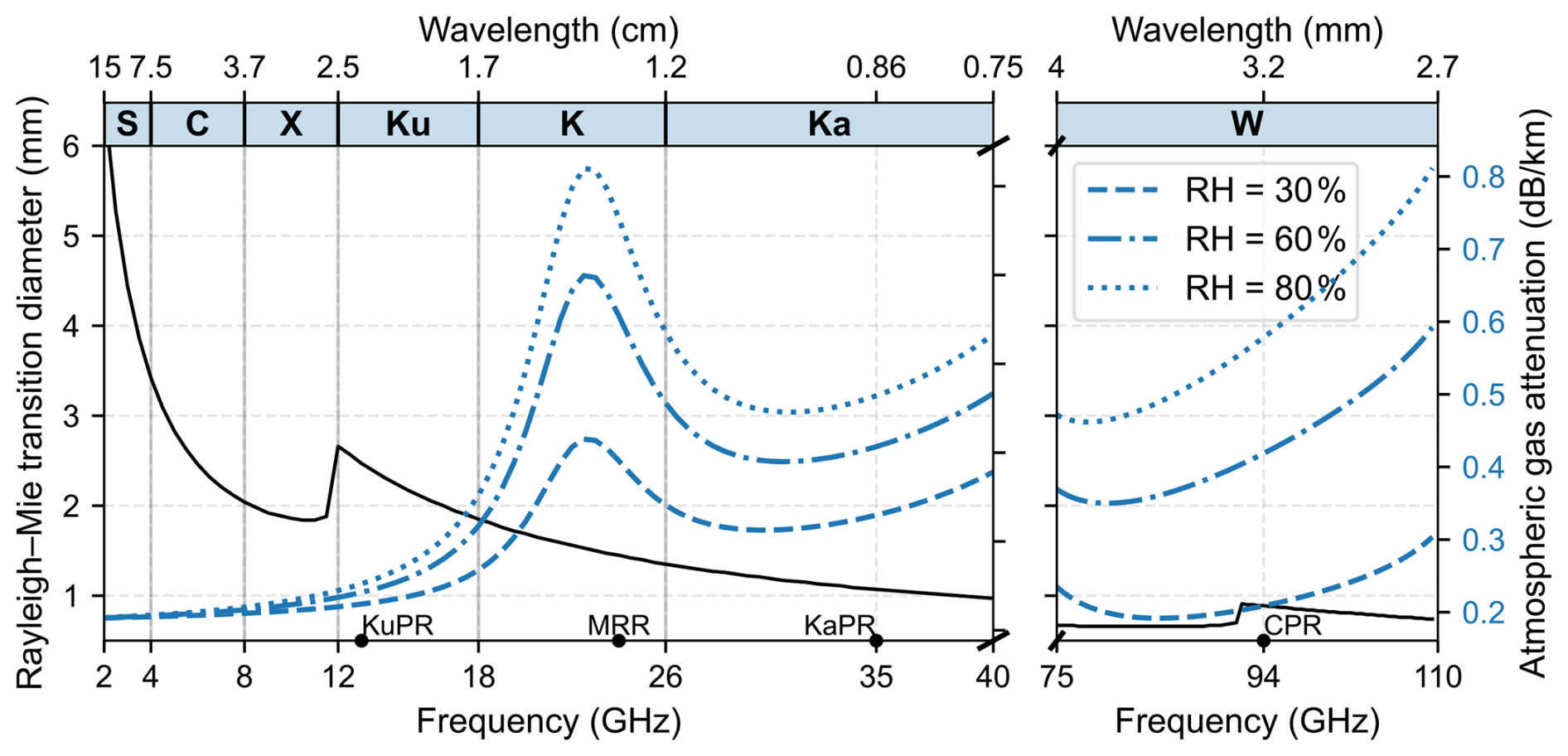
Figure E1 Frequency dependence of the Rayleigh–Mie transition diameter and atmospheric gas attenuation (oxygen and water vapor) across microwave radar bands. The bottom x-axis shows frequency (GHz) and the top axes show the corresponding wavelengths (cm and mm), with S, C, X, Ku, K, Ka, and W bands indicated. The operating frequencies of TRMM and GPM KuPR, MRR, GPM KaPR, and CloudSat and EarthCARE CPR radars are annotated. The black solid curve (left y-axis) represents the drop diameter at which scattering transitions from the Rayleigh to the Mie regime. The transition is defined as the diameter at which the pytmatrix-simulated normalized radar backscattering cross section $\frac{{\mathit{\sigma }}_{\mathrm{H}}^{\mathrm{b}}\left(D\right)}{\mathit{\pi }(D/\mathrm{2}{)}^{\mathrm{2}}}$ deviates by more than 10 % from the Rayleigh approximation. The blue dashed, dash-dotted, and dotted curves (right y-axis) show atmospheric gas attenuation (dB km⁻¹) for relative humidity (RH) levels of 30 %, 60 %, and 80 %, respectively. Gaseous attenuation increases with both frequency and humidity, exhibits a pronounced peak near the 22–24 GHz water vapor absorption band, and becomes very strong in the oxygen absorption region within the V band (40–75 GHz; not shown). Strong gaseous attenuation also occurs at W band frequencies.

E1.5 Linear depolarization ratio

The linear depolarization ratio LDR measures the power returned in the cross-polar channel relative to the copolar channel, providing insight into deviations from spherical symmetry and fluctuations in particle orientation:

$$\begin{array}{}\text{(E12)}& \begin{array}{rl}\mathrm{LDR}& =\mathrm{10}{\log }_{\mathrm{10}}\left({\displaystyle \frac{{\int }_{D_{min}}^{D_{max}}\left|s_{\mathrm{VH}}^{\mathrm{b}}\right(D\left){|}^{\mathrm{2}}N\right(D)\mathrm{d}D}{{\int }_{D_{min}}^{D_{max}}\left|s_{\mathrm{HH}}^{\mathrm{b}}\right(D\left){|}^{\mathrm{2}}N\right(D)\mathrm{d}D}}\right)\\ & =\mathrm{10}{\log }_{\mathrm{10}}\left({\displaystyle \frac{{\int }_{D_{min}}^{D_{max}}{\mathit{\sigma }}_{\mathrm{VH}}^{\mathrm{b}}\left(D\right)N\left(D\right)\mathrm{d}D}{{\int }_{D_{min}}^{D_{max}}{\mathit{\sigma }}_{\mathrm{HH}}^{\mathrm{b}}\left(D\right)N\left(D\right)\mathrm{d}D}}\right)\left[\mathrm{dB}\right]\end{array}\end{array}$$

E2 Forward scattering radar variables

Propagation-related quantities are derived from the forward-scattering amplitude coefficients evaluated at the forward direction (θ_s=0°).

E2.1 Specific propagation differential phase

The specific propagation differential phase K_DP is the rate of change in phase between horizontal and vertical transmitted pulses, caused primarily by oriented, non-spherical hydrometeors:

$$\begin{array}{}\text{(E13)}& \begin{array}{rl}{K}_{\mathrm{DP}}& ={\displaystyle \frac{\mathrm{180}}{\mathit{\pi }}}{\mathrm{10}}^{-\mathrm{3}}\mathit{\lambda }\underset{D_{min}}{\overset{D_{max}}{\int }}Re\left[s_{\mathrm{HH}}^{\mathrm{f}}\right(D)\\ & -s_{\mathrm{VV}}^{\mathrm{f}}\left(D\right)\left]N\right(D\left)\mathrm{d}D\right[\mathit{°}{\text{km}}^{-\mathrm{1}}]\end{array}\end{array}$$

with the factor 10⁻³ used to convert mm² m⁻³ to km⁻¹. K_DP is highly valuable for rainfall estimation because it is immune to radar calibration errors and partial beam blockage, and has a nearly linear relationship with the rain rate and specific attenuation in moderate to heavy rainfall. Similarly to Z_DR, K_DP also decreases with increasing canting angle spread because greater orientation randomness reduces the anisotropy of forward scattering between horizontally and vertically polarized waves.

E2.2 Specific attenuation

Specific attenuation quantifies the rate at which the radar signal is weakened by extinction (scattering and absorption) as it propagates through the hydrometeor population:

$$\begin{array}{}\text{(E14)}& {\displaystyle }{A}_{\mathrm{H}}=\mathrm{4.343}{\mathrm{10}}^{-\mathrm{3}}\underset{D_{min}}{\overset{D_{max}}{\int }}{\mathit{\sigma }}_{\mathrm{H}}^{\mathrm{ext}}N\left(D\right)\mathrm{d}D\left[{\text{dB\hspace{0.17em}km}}^{-\mathrm{1}}\right]\text{(E15)}& {\displaystyle }{A}_{\mathrm{V}}=\mathrm{4.343}{\mathrm{10}}^{-\mathrm{3}}\underset{D_{min}}{\overset{D_{max}}{\int }}{\mathit{\sigma }}_{\mathrm{V}}^{\mathrm{ext}}N\left(D\right)\mathrm{d}D\left[{\text{dB\hspace{0.17em}km}}^{-\mathrm{1}}\right]\end{array}$$

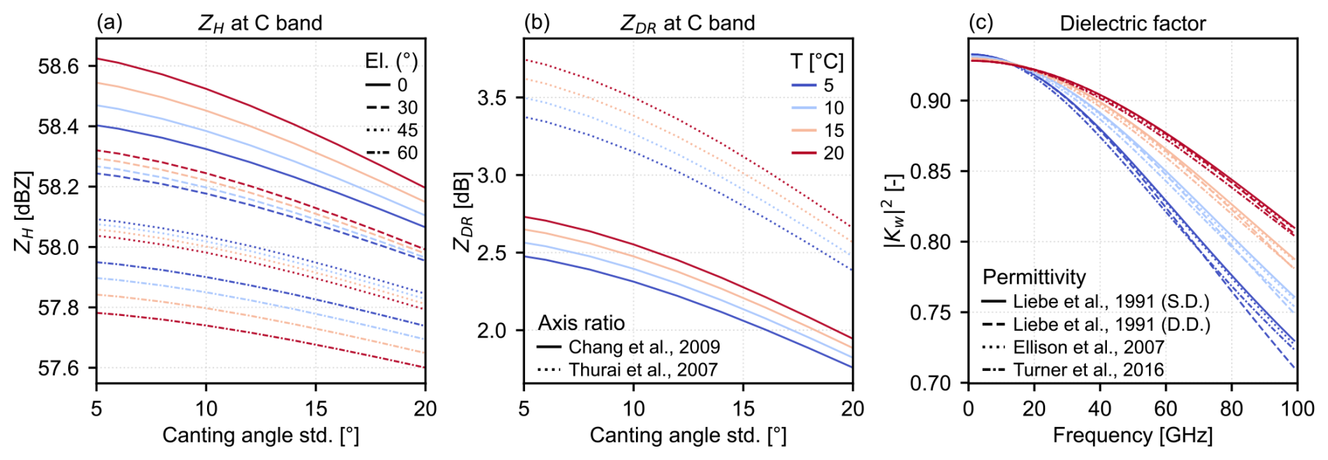
Figure E2 Sensitivity of polarimetric radar variables to particle orientation variability, drop water temperature, and radar scanning geometry, and variability of the dielectric factor with frequency and temperature. The DSD shown in Fig. 8b, c is used for this sensitivity experiment. (a) Simulated horizontal reflectivity Z_H at C band as a function of the standard deviation of a Gaussian canting angle distribution (zero mean), for drop temperatures of 5–20 °C and radar elevation angles of 0, 30, 45, and 60°. Z_H slightly decreases with increasing canting angle spread and elevation angle. In the Rayleigh regime (e.g., S band), the effect of drop temperature on Z is negligible. In the Mie regime (e.g., C band for large drops and X band), temperature-dependent changes in the complex dielectric constant modify the drop backscattering cross section and thus Z, potentially producing nonlinear or non-monotonic behavior. (b) Corresponding differential reflectivity Z_DR at C band and 0° elevation as a function of canting angle spread for temperatures of 5–20 °C, using axis-ratio models from Chang et al. (2009) and Thurai et al. (2007). Z_DR decreases with increasing canting angle variability because greater orientation randomness reduces the difference between horizontally and vertically polarized backscatter. Z_DR also decreases with increasing radar elevation angle (not shown) as the viewing geometry becomes less sensitive to the horizontal oblateness of raindrops. (c) Magnitude of the dielectric factor $|K_{\mathrm{w}}{|}^{\mathrm{2}}$ for liquid water as a function of frequency (0–100 GHz) and temperature, computed using permittivity models from Liebe et al. (1991) (single- and double-Debye), Ellison (2007), and Turner et al. (2016).

The factor 4.343 (10 log ₁₀(e)) arises from converting the natural-logarithmic form of extinction in the Beer–Lambert law to the decibel scale (Bringi and Chandrasekar, 2001).

E2.3 Differential attenuation

Differential attenuation quantifies the difference in specific attenuation between horizontal and vertical polarizations:

$$\begin{array}{}\text{(E16)}& A_{\mathrm{DP}}=A_{\mathrm{H}}-A_{\mathrm{V}}\left[{\text{dB\hspace{0.17em}km}}^{-\mathrm{1}}\right]\end{array}$$

In rainfall, A_DP increases with drop size and oblateness, as larger raindrops attenuate the horizontally polarized wave more strongly than the vertically polarized one.