Towards a remote sensing solution to quantify nitrous oxide emissions by integrating shortwave and thermal infrared bands

Nitrous oxide (N₂O) is a potent greenhouse gas whose emissions are dominated by natural and agricultural soils and are highly heterogeneous and episodic, yet existing observational techniques lack the spatial coverage and near-surface sensitivity needed to resolve this variability. In this study, we evaluate a remote sensing framework that integrates shortwave infrared (SWIR) and thermal infrared (TIR) spectral bands to enhance the detectability of column-integrated N₂O mixing ratio ($X_{{\mathrm{N}}_{\mathrm{2}}\mathrm{O}}$). To implement this, we expand the capacity of Smithsonian PLanetary ATmosphere–Vector Linearized Discrete Ordinate Radiative Transfer (SPLAT–VLIDORT) model to jointly simulate both spectral regions and apply linear sensitivity analysis to quantify the $X_{{\mathrm{N}}_{\mathrm{2}}\mathrm{O}}$ measurement error and vertical sensitivity under realistic environmental conditions and instrumental designs. This framework is applied to both airborne and spaceborne instruments to evaluate the influence of platform characteristics on retrieval performance. The joint SWIR–TIR setting improves near-surface sensitivity relative to the TIR band alone while maintaining the low $X_{{\mathrm{N}}_{\mathrm{2}}\mathrm{O}}$ measurement error. It achieves single-sounding measurement error of approximately 3.2 ppb for an airborne instrument with a ground footprint size of 20 m and 1.1 ppb for spaceborne instrument with a footprint size of 0.7 km, while retaining sensitivity to the near-surface layers. Assuming $X_{{\mathrm{N}}_{\mathrm{2}}\mathrm{O}}$ variability is observable at twice the precision, natural $X_{{\mathrm{N}}_{\mathrm{2}}\mathrm{O}}$ variability inferred from in situ aircraft N₂O observations in the US Midwest becomes observable beyond spatial aggregation scales of ∼2.5 km for airborne and ∼22 km for spaceborne instruments, subject to significant $X_{{\mathrm{N}}_{\mathrm{2}}\mathrm{O}}$ variation between flights. An independent, emission-based detectability analysis indicates that $X_{{\mathrm{N}}_{\mathrm{2}}\mathrm{O}}$ variability induced by uniform emissions of 5 nmol m⁻² s⁻¹ becomes observable beyond spatial averaging of about 2.1 km for airborne and 8.4 km for spaceborne instruments. Together, these results constitute a quantitative basis for N₂O detectability using a joint SWIR–TIR setting, with a focus on diffuse soil emissions that are more difficult to detect yet dominate the global N₂O budget, and they provide practical guidance for future N₂O dedicated missions.

1 Introduction

Nitrous oxide (N₂O) is the third most important anthropogenic greenhouse gas after carbon dioxide (CO₂) and methane (CH₄) (Weber et al., 2024; Feng and Li, 2023), currently accounting for approximately 7 % of the net anthropogenic radiative forcing (3.22 W m⁻²) of the Earth's climate system (Feng and Li, 2023; IPCC, 2021). It has a global warming potential of roughly 273 times greater than CO₂ over a 100-year timescale (Weber et al., 2024) and an atmospheric lifetime of 116 ± 9 years (Prather et al., 2015), primarily due to its slow removal via photolysis in the stratosphere (Tian et al., 2020). Anthropogenic activities including fuel combustion, agriculture, and industrial processes have substantially increased the N₂O emissions (Smith, 2017; Jovani-Sancho et al., 2023), with nitrogen-based fertilizers used in agriculture being the major contributor (Thompson et al., 2019; Tian et al., 2020). In the global N₂O budget at about 19 Tg N yr⁻¹, natural soil emissions dominate the N₂O sources at about 6–7 Tg N yr⁻¹, followed by agricultural emissions ranging from 4.3 to 5.8 Tg N yr⁻¹ (Syakila and Kroeze, 2011). Atmospheric N₂O concentrations have already exceeded those projected under the most pessimistic scenario of the Shared Socioeconomic Pathway (SSP5-8.5), suggesting that current emission trajectories surpass both policy expectations and model projections (Tian et al., 2024). This is further reinforced by Microwave Limb Sounder (MLS) observations from 2005–2021, which reveal a growing stratospheric sink for N₂O, implying that actual emissions may be higher than those inferred from concentration data alone (Prather et al., 2023).

A variety of observational techniques have been used to quantify N₂O emissions and characterize their spatiotemporal variability. Chambers are widely employed for agricultural field-scale studies (Zhang et al., 2024; Kong et al., 2025; Zimbron et al., 2025), offering high precision at fine temporal resolution, but they are effectively point measurements and are not representative of broader heterogeneous landscapes. Ground-based Eddy Covariance (EC) systems provide continuous flux measurements over larger footprints (∼1 km² scale), capturing ecosystem-scale dynamics, but their fixed-point nature limits spatial coverage (Murphy et al., 2022; Pan et al., 2022; Rana et al., 2025; Tikkasalo et al., 2025). Airborne EC campaigns overcome this limitation by measuring fluxes over tens to hundreds of kilometers and have been particularly effective in agricultural regions, although their deployment remains logistically complex and resource-intensive (Wilkerson et al., 2019; Waldmann et al., 2026). Similarly, airborne or tall tower-based in situ measurements combined with atmospheric transport and inversion models provide valuable top-down estimates of regional emissions, offering a complement to inventory-based approaches (Dacic et al., 2024; Gvakharia et al., 2020; Xiang et al., 2013; Griffis et al., 2019; Haszpra et al., 2018; Kort et al., 2011; Chen et al., 2016b). Despite these advances, accurately capturing soil N₂O emissions, complicated by their episodic and spatially heterogeneous nature (Molodovskaya et al., 2012; Ackett et al., 2025; Zhang et al., 2024; Zhou et al., 2022; Shrestha and Wang, 2018), remains a major challenge, underscoring the need for scalable observational strategies with improved spatial resolution.

Remote sensing of greenhouse gases on spaceborne or airborne platforms offers a powerful alternative to overcome these spatiotemporal limitations, by providing coverage up to the global scale and allowing the detection of long-term trends and multiscale emission patterns (Jacob et al., 2016). Remote sensing instruments typically observe the dry air column-integrated mixing ratio of greenhouse gases, conventionally denoted as “X” followed by the molecule name, e.g., $X_{{\mathrm{N}}_{\mathrm{2}}\mathrm{O}}$ for N₂O. These column amounts are insensitive to the vertical distributions of trace species and thus more closely related to emissions than point-based volume mixing ratios (Chen et al., 2016a). Over the recent decade, missions such as the Orbiting Carbon Observatories (OCO-2 & OCO-3) (Crisp, 2015; Crisp et al., 2017; Eldering et al., 2019; Taylor et al., 2023), TROPOspheric Monitoring Instrument (TROPOMI) (Lorente et al., 2021), Greenhouse Gases Observing Satellite (GOSAT) series (Butz et al., 2011; Suto et al., 2021), and MethaneSAT (South, 2024) deliver high-precision $X_{{\mathrm{CO}}_{\mathrm{2}}}$ and $X_{{\mathrm{CH}}_{\mathrm{4}}}$ retrievals and have demonstrated the ability to detect and quantify emissions from global to sub-kilometer scales. Airborne platforms provide complementary capabilities by targeting high-resolution observations at finer spatial scales. For example, MethaneAIR, an airborne precursor to MethaneSAT, provides a fine spatial resolution of 20 × 20 m² with overall $X_{{\mathrm{CH}}_{\mathrm{4}}}$ retrieval accuracy within ∼ 1 % when validated against ground-based spectrometers (Chan Miller et al., 2024; Chulakadabba et al., 2023).

In contrast, there exists no dedicated remote sensing mission for N₂O (Ricaud et al., 2021). In the shortwave infrared (SWIR) spectral region, where CO₂ and CH₄ instruments have achieved remarkable success, the most detectable N₂O band near 2.3 µm is weak and subject to significant interference from CH₄ bands. Stronger N₂O features are found in the thermal infrared (TIR) near 4.4 or 7.8 µm, but TIR observations have limited sensitivity to near-surface layers, which matter the most for emission detection. In addition, the relative emission-induced enhancements to the N₂O column are generally lower than those of CH₄ and CO₂, and in this regard, N₂O has been proposed as a light-path proxy for CH₄ and CO₂ retrievals (Frankenberg et al., 2025). For example, the peak-to-peak variability of N₂O volume mixing ratio observed in the planetary boundary layer (PBL) over a source region is only a few ppb (Dacic et al., 2024), which translates to an $X_{{\mathrm{N}}_{\mathrm{2}}\mathrm{O}}$ variability of about 1 ppb, or 0.3 % of the $X_{{\mathrm{N}}_{\mathrm{2}}\mathrm{O}}$ background. This makes N₂O sources more difficult to detect than CO₂ or CH₄ even given comparable instrument sensitivity. As secondary products, N₂O abundance has been retrieved from existing satellite-observed spectra in both SWIR and TIR bands. The SCanning Imaging Absorption SpectroMeter for Atmospheric CHartographY (SCIAMACHY) offered one of the first N₂O detection capabilities in SWIR region. With a target precision of approximately 10 % in the retrieved N₂O column amount, the SCIAMACHY N₂O product is insufficient for detecting localized enhancements (Dils et al., 2006). Infrared sounders primarily designed for numerical weather prediction, such as the Atmospheric Infrared Sounder (AIRS) and the Infrared Atmospheric Sounding Interferometer (IASI), have improved upon SCIAMACHY with typical N₂O precision close to 1 % (Xiong et al., 2014; Vandenbussche et al., 2022). However, their coarse spatial resolution and limited near-surface sensitivity make them poorly suited for detecting localized N₂O emission sources. For the first time, the GOSAT-2 satellite covers both SWIR and TIR N₂O bands with the same instrument, but its coarse footprint diameter of ∼10 km and sparse sampling geometry limit its ability to resolve localized and spatially heterogeneous N₂O enhancements (Suto et al., 2021). Using only the SWIR N₂O band of GOSAT-2, Noël et al. (2022) provided the first $X_{{\mathrm{N}}_{\mathrm{2}}\mathrm{O}}$ product from GOSAT-2 with single-sounding precisions of about 4–9 ppb. Still, current spaceborne N₂O instrumentation cannot be used to study agricultural emissions, which triggers attempts to use other high-resolution nitrogen species as a proxy (Adams et al., 2026).

Leveraging the heritages of existing greenhouse gas instruments, especially MethaneAIR and MethaneSAT, this study presents a dual SWIR–TIR band concept applicable for both airborne and spaceborne N₂O remote sensing instruments. Similar to MethaneAIR and MethaneSAT, this concept employs high spatial resolution (footprint sizes of about 20 m for airborne and 0.7 km for spaceborne instruments), wide swath imaging grating spectrometer designs for the ability to detect both emission hot spots (Warren et al., 2025) and dispersed sources (MacKay et al., 2026). The coverage of the SWIR N₂O band at 2.3 µm offers near-uniform vertical sensitivity desirable for emission quantification. The TIR N₂O band at 7.8 µm is selected to provide crucial observational constraints to $X_{{\mathrm{N}}_{\mathrm{2}}\mathrm{O}}$, additional to the weak SWIR band. Although N₂O exhibits much stronger absorption features near 4.4 µm, the 7.8 µm region was selected to avoid mixed solar–thermal radiance contributions and potential non-Local Thermodynamic Equilibrium (non-LTE) effects (Barnet et al., 2023). For the first time, we enhance the Smithsonian PLanetary ATmosphere–Vector Linearized Discrete Ordinate Radiative Transfer (SPLAT–VLIDORT), the radiative transfer model underpinning the MethaneAIR and MethaneSAT retrieval algorithms (Chan Miller et al., 2024), to enable a joint SWIR–TIR retrieval. Linear sensitivity analysis based on this enhanced radiative transfer framework demonstrates that the integration of SWIR and TIR bands yields significantly improved N₂O precision and PBL sensitivity relative to the limiting single-band case, an advantage similarly seen in the multispectral CO retrieval in the Measurements of Pollution in the Troposphere (MOPITT) instrument (Worden et al., 2010).

To assess the N₂O detectability by the proposed instruments under realistic conditions, we approximate real-world $X_{{\mathrm{N}}_{\mathrm{2}}\mathrm{O}}$ variability in two complementary ways. The first is to assume $X_{{\mathrm{N}}_{\mathrm{2}}\mathrm{O}}$ covaries with PBL N₂O mixing ratio, which was extensively sampled by an aircraft during the Measurement of Agriculture Illuminating farm-Zone Emissions of N₂O (MAIZE) campaign over the US Midwest. The second is to transform a range of hypothetical N₂O emissions that are informed by autochamber flux data to $X_{{\mathrm{N}}_{\mathrm{2}}\mathrm{O}}$ enhancements at various spatial scales. These $X_{{\mathrm{N}}_{\mathrm{2}}\mathrm{O}}$ variabilities are then compared with $X_{{\mathrm{N}}_{\mathrm{2}}\mathrm{O}}$ measurement error at common spatial scales to infer detectability. Together, these results establish the scientific basis for N₂O remote sensing missions dedicated to detect and quantify agricultural soil N₂O emissions at spatial scales relevant to emissions monitoring and management, providing practical guidance for instrument design aimed at closing existing gaps in N₂O monitoring. By treating agricultural N₂O emissions as the primary design case, the proposed instrument capable of resolving the most challenging sources will also be well suited for other stronger emission sectors such as industrial.

2 Data

This section presents the three observational datasets used in this study. First, satellite-retrieved atmospheric state data from the Cross-track Infrared Sounder (CrIS) provide surface temperature, profiles of key absorbers (N₂O, CH₄, and H₂O) and temperature, along with the surface emissivity used for the TIR band simulations. For SWIR, a representative grass albedo from the Terra Advanced Spaceborne Thermal Emission and Reflection Radiometer (ASTER) climatology is assumed, with values ranging from 0.146 to 0.171 over the selected SWIR spectral window. These quantities define the atmospheric and surface conditions for forward radiative transfer modeling (Sect. 3.1.4) in the SWIR and TIR spectral regions and allow estimation of prior error structures (Sect. 3.1.2). In combination with the instrument noise characteristics (Sect. 3.1.3), these lead to the $X_{{\mathrm{N}}_{\mathrm{2}}\mathrm{O}}$ measurement error estimation for the proposed instruments. Second, airborne in-situ measurements from the MAIZE campaign (Sect. 2.2) capture high-resolution N₂O variability within the PBL over a major agricultural region, shedding light on the $X_{{\mathrm{N}}_{\mathrm{2}}\mathrm{O}}$ spatial heterogeneity using semivariograms (Sect. 3.2). Although the CrIS and MAIZE datasets are not colocated in time and space, both are representative of summertime agricultural conditions over the US Midwest dominated primarily by corn and soybean croplands. These datasets are used as complementary constraints for realistic environmental variability rather than for direct scene-by-scene comparison. Third, hourly N₂O flux measurements by autochambers distributed in a commercial farm in Illinois (Sect. 2.3) provide realistic spatiotemporal variability of soil N₂O emissions, putting the detectability of N₂O emissions into a real-world context (Sect. 3.3).

2.1 Realistic geophysical quantities from CrIS Level 2 product

Level 2 data from the CrIS instrument onboard NOAA's JPSS satellites are used to construct realistic profiles of trace gases (N₂O, CH₄, H₂O) and temperature as well as surface temperature and emissivity useful for the TIR radiative transfer modeling. This study leverages 100 CrIS soundings over the US Midwest acquired on 23 August 2023. The selected date provides a large number of clear-sky soundings spanning a wide range of thermal contrast (2–12 K), providing a representative sample of US Midwest summertime conditions for evaluating retrieval sensitivity. Figure 1 shows the spatial distribution of the selected CrIS pixels, color-coded by thermal contrast, which is defined as the difference between retrieved surface temperature and that of the lowest atmospheric layer. The selected region in Fig.1 is dominated by agricultural land cover, primarily corn and soybean croplands. Thermal contrast is most important for the TIR band, as it governs the strength of the upwelling signal and thus influences vertical sensitivity. The prior error matrices for H₂O and temperature profiles available in the CrIS Level 2 data are used to set a priori constraints in the linear sensitivity study (see Sect. 3.1.2).

Figure 1 Spatial distribution of 100 CrIS soundings over the US Midwest on 23 August 2023, color-coded by thermal contrast. These pixels span a wide range of thermal contrast from 2–12 K.

2.2 MAIZE aircraft campaign in situ measurements

Airborne in-situ measurements of N₂O were conducted over the state of Iowa, located within the corn belt of United States (41 to 43.5° N and 92 to 95° W), in 2022 as part of the MAIZE campaign. A total of eight research flights took place between 18 and 30 May 2022 using a Mooney aircraft operated by Scientific Aviation, Inc. Flights were conducted during growing season under fair weather conditions, avoiding active precipitation, low visibility events, and on days with steady winds. This period, characterized by recent fertilizer application and warm and moist conditions was conducive to elevated N₂O emissions from cropland soils. Each flight lasted around 5–6 h and was conducted between 11:00 and 18:00 local time to ensure sampling within a well-developed PBL. The aircraft flew at an average altitude of ∼ 475 m above ground level (a.g.l.), with transects oriented perpendicular to the prevailing wind direction to enhance sensitivity to surface fluxes. Two vertical profiles were captured during each flight to characterize the PBL structure. The primary target species, N₂O, was measured using a Los Gatos Research (LGR) N₂O/CO Analyzer (model 916‐0015), which also recorded H₂O and CO. In addition, CH₄ and CO₂ were measured using a Picarro G2401–m analyzer (Dacic et al., 2024). The N₂O in situ measurements are used to approximate column-integrated mixing ratio of N₂O and analyze its spatial variability. Figure 2a shows the area coverage for each flight and Fig. 2b indicates the corresponding in situ N₂O mixing ratios measured during each flight. Figure 2b has two vertical axes, with the left and right axes showing in situ N₂O mixing ratio in ppb for alternating flights to improve readability. In both panels, faint lines indicate vertical profile segments and bold lines mark the horizontal PBL transects used to quantify $X_{{\mathrm{N}}_{\mathrm{2}}\mathrm{O}}$ variability for the semivariogram-based detectability analysis.

Figure 2 (a) Flight tracks during the MAIZE campaign over the state of Iowa in May 2022. (b) Corresponding time series of in situ N₂O mixing ratios. Both vertical axes represent the in situ N₂O mixing ratio in ppb. The left and right axes are used for alternating flight days to reduce overlap and improve readability. In both panels, faint lines represent vertical profile segments, while bold lines highlight horizontal flight path within the PBL used to calculate $X_{{\mathrm{N}}_{\mathrm{2}}\mathrm{O}}$ variability for detectability analysis. Colors distinguish individual flight days and are consistent between panels.

2.3 Autochamber flux data

Hourly N₂O fluxes were measured from May 2022 to April 2023 in a conventionally-tilled maize field near Villa Grove, Illinois, using 16 automated chambers. To capture spatial and temporal variability of emissions, the chambers were distributed across four sampling nodes within ∼ 5 ha area, with nodes spaced 50–100 m apart (Fig. 3a inset). Each node contained four chambers radially positioned 12 m from a central N₂O gas analyzer (LI-7820, LI-COR Biosciences), which sequentially sampled the fluxes using an automated multiplexer (LI-8250). Chamber collars (20 cm diameter) were permanently installed adjacent to crop rows, ensuring that no vegetation was present within the chamber footprint and that chambers remained fully open between measurements in order to avoid shading or disturbance. Figure 3a shows the spatiotemporal variation of measured N₂O flux across four nodes, where chambers in the same node are averaged and then aggregated to 6 h intervals to enhance visualization. Data are missing for approximately three weeks in October–November 2022 due to instrument maintenance and crop harvest (Stuchiner et al., 2025). Figure 3b zooms in over a high emission event of 21–25 May 2022 to highlight the hourly variability of N₂O emissions. The node-wise average time series are shown as solid lines, while the maximum and minimum chamber values within each node are shown as dashed lines. The thick grey line represents the overall hourly flux averaged over all nodes which remain mostly above 5 nmol m⁻² s⁻¹ and occasionally exceed 10 nmol m⁻² s⁻¹ in this period.

Figure 3 Time series of soil N₂O flux (nmol m⁻² s⁻¹) measured from May 2022 to April 2023 using automated chambers deployed at four nodes in a conventionally tilled maize field near Villa Grove, Illinois. (a) Node-averaged fluxes at 6-hourly resolution showing the temporal and spatial variability, with distinct emission pulses during the early growing season. The inset shows the spatial arrangement of nodes and chambers within an area of ∼ 5 ha. (b) Expanded view of 21–25 May 2022, highlighting the hourly flux variability. Solid lines represent node-averaged fluxes, dashed lines denote the minimum and maximum chamber values within each node, and the thick grey line represents the average across all nodes.

3 Measurement Methodology

This section combines theoretical analysis and empirical data to evaluate the capability of potential dual-band remote sensing instruments for detecting N₂O emissions on both airborne and spaceborne platforms. Section 3.1 introduces the linear sensitivity analysis framework, which takes a Bayesian approach to quantify $X_{{\mathrm{N}}_{\mathrm{2}}\mathrm{O}}$ measurement error and vertical sensitivity based on instrument design parameters, a priori constraints, and radiative transfer simulations. Section 3.2 leverages in situ airborne N₂O measurements from the MAIZE campaign to approximate spatial variability of $X_{{\mathrm{N}}_{\mathrm{2}}\mathrm{O}}$ and characterize how this variability compares with measurement error at different spatial scales. Finally, Sect. 3.3 compares emission-driven column enhancement against measurement error. Both Sect. 3.2 and 3.3 aim to provide a quantitative basis for the detectability of N₂O emissions by the proposed instruments.

3.1 Linear sensitivity analysis

3.1.1 Theory

As articulated in Rodgers (2000), the linear sensitivity analysis framework assumes that the perturbations to a vector of observations y are linear relative to the perturbations of a state vector x. In other words, the Jacobian

$$\begin{array}{}\text{(1)}& \mathbf{K}={\displaystyle \frac{\partial \mathit{y}}{\partial \mathit{x}}}\end{array}$$

is approximately constant within the error range of x. Here, y is the expected values of a spectrum observed by a remote sensing instrument with Gaussian spectral error covariance matrix S_o, and the state vector consists of the volume mixing ratio profiles of N₂O, CH₄, and H₂O, atmospheric temperature profile, and the surface temperature. We assume a priori knowledge of x as a Gaussian distribution with mean value x_a and a covariance matrix of S_a. Within the Bayesian framework, S_a represents the prior uncertainty of the state vector. Practically, it also acts as a regularization whose strength can be controlled by multiplying S_a by a scaling factor, as implemented in Sect. 4.1. The a priori profiles are adopted from CrIS Level 2 products as mentioned in Sect. 2.1. The prior error matrices are constructed in a similar manner to those deployed in the MethaneAIR/GOSAT algorithms for N₂O and CH₄ profiles and extracted from CrIS Level 2 product for H₂O and atmospheric temperature profiles (see Sect. 3.1.2). The spectral error covariance matrix S_o is constructed based on the instrument specification given in Sect. 3.1.3. The Jacobian K is calculated using the radiative transfer model detailed in Sect. 3.1.4.

Applying the Bayes' theorem, the state vector can be retrieved from the observation and the prior:

$$\begin{array}{}\text{(2)}& \widehat{\mathit{x}}={\mathit{x}}_{\mathrm{a}}+\mathbf{G}(\mathit{y}-\mathbf{K}{\mathit{x}}_{\mathrm{a}}),\end{array}$$

where

$$\begin{array}{}\text{(3)}& \mathbf{G}={\displaystyle \frac{\partial \widehat{\mathit{x}}}{\partial \mathit{y}}}={\mathbf{S}}_{\mathrm{a}}{\mathbf{K}}^{\mathrm{T}}{\left({\mathbf{KS}}_{\mathrm{a}}{\mathbf{K}}^{\mathrm{T}}+{\mathbf{S}}_{\mathrm{o}}\right)}^{-\mathrm{1}}\end{array}$$

is the gain matrix. Here, T denotes matrix transpose. The measurement error is linearly propagated from the observation to the retrieved state vector:

$$\begin{array}{}\text{(4)}& {\mathbf{S}}_{\mathrm{m}}={\mathbf{GS}}_{\mathrm{o}}{\mathbf{G}}^{\mathrm{T}}.\end{array}$$

Our goal is to retrieve $X_{{\mathrm{N}}_{\mathrm{2}}\mathrm{O}}$, which can be written as a function of the retrieved state vector:

$$\begin{array}{}\text{(5)}& X_{{\mathrm{N}}_{\mathrm{2}}\mathrm{O}}={\mathit{h}}^{\mathrm{T}}\widehat{\mathit{x}}.\end{array}$$

Currently, we assume $X_{{\mathrm{N}}_{\mathrm{2}}\mathrm{O}}$ only depends on the retrieved N₂O mixing ratio profile, so the weighting vector h is the fractional dry air column at the corresponding layers of the N₂O profile and zero for all other elements of the state vector, such that only N₂O profile contributes to the calculation of $X_{{\mathrm{N}}_{\mathrm{2}}\mathrm{O}}$. The measurement error of $X_{{\mathrm{N}}_{\mathrm{2}}\mathrm{O}}$ is then linearly propagated from the state vector measurement error:

$$\begin{array}{}\text{(6)}& {\mathit{\sigma }}_{X_{{\mathrm{N}}_{\mathrm{2}}\mathrm{O}}}={\mathit{h}}^{\mathrm{T}}{\mathbf{S}}_{\mathrm{m}}\mathit{h}.\end{array}$$

This measurement error, or precision of $X_{{\mathrm{N}}_{\mathrm{2}}\mathrm{O}}$, is influenced by interference errors associated with the variabilities and sensitivities of the other retrieved state vector elements through the gain matrix (Connor et al., 2016). However, the interference errors from the non-N₂O state vector elements are at least one order of magnitude smaller than the N₂O measurement error, indicating that their contributions are minimal compared to the dominant N₂O measurement uncertainty. ${\mathit{\sigma }}_{X_{{\mathrm{N}}_{\mathrm{2}}\mathrm{O}}}$ is a fundamental design parameter for any N₂O instrument as it limits the observable variability of $X_{{\mathrm{N}}_{\mathrm{2}}\mathrm{O}}$ by instrument noise. However, ${\mathit{\sigma }}_{X_{{\mathrm{N}}_{\mathrm{2}}\mathrm{O}}}$ does not inform the different detectability at different part of the atmosphere. When the a priori is dominant, the retrieval precision mostly reflects the a priori uncertainty. As such, we will leverage the averaging kernel matrix, which represents the sensitivity of the retrieved state to the true atmosphere state and is given by

$$\begin{array}{}\text{(7)}& \mathbf{A}={\displaystyle \frac{\partial \widehat{\mathit{x}}}{\partial \mathit{x}}}=\mathbf{GK}.\end{array}$$

$X_{{\mathrm{N}}_{\mathrm{2}}\mathrm{O}}$ as a derived quantity from the retrieved state can then be evaluated using the column averaging kernel vector a. The element of the column averaging kernel for the lth N₂O layer is

$$\begin{array}{}\text{(8)}& {\mathit{a}}_l={\displaystyle \frac{\mathrm{1}}{{\mathit{h}}_l}}({\mathit{h}}^{\mathrm{T}}\mathbf{A}{)}_l,\end{array}$$

in which the subscript l only indexes the elements related to the N₂O profile. For a particular layer, a column averaging kernel value equaling 1 represents the ideal case, where the retrieved $X_{{\mathrm{N}}_{\mathrm{2}}\mathrm{O}}$ responds to changes in N₂O mixing ratio profile exactly as the true value of $X_{{\mathrm{N}}_{\mathrm{2}}\mathrm{O}}$. A column averaging kernel value smaller than 1 indicates that the retrieved $X_{{\mathrm{N}}_{\mathrm{2}}\mathrm{O}}$ is less sensitive to N₂O in that layer, and that the a priori N₂O profile element is a significant contributor. We use the mean column averaging kernel values of the bottom two layers (roughly the bottom 1 km) as the indicator of the retrieved $X_{{\mathrm{N}}_{\mathrm{2}}\mathrm{O}}$'s sensitivity to near-surface N₂O. A desirable instrument design should have a low $X_{{\mathrm{N}}_{\mathrm{2}}\mathrm{O}}$ measurement error and a near-surface column averaging kernel value close to 1.

3.1.2 A priori constraint

The prior error covariance matrix S_a is a crucial element in the regularization of the retrieval, as it balances the contributions from the observation and the prior. Since no mature operational N₂O covariance structure is currently available, we adopt the MethaneAIR CH₄ a priori error covariance matrix (Chan Miller et al., 2024), which originates from the GOSAT CH₄ algorithm developed by the University of Leicester (Parker et al., 2020), for both N₂O and CH₄ profiles. Similar to Chan Miller et al. (2024), we decompose the error covariance matrix into a standard deviation profile and an error correlation matrix. The N₂O standard deviation profile, shown in Fig. 4a, is scaled down from the original CH₄ standard deviation profile by a factor of 5.76 based on the ratio between typical atmospheric abundance of CH₄ (∼ 1900 ppb) and N₂O (∼ 330 ppb), reflecting the lower atmospheric abundance of N₂O. The purpose of adopting this scaled CH₄ prior covariance structure here is not to reproduce the exact climatological variability of atmospheric N₂O, which is expected to be smaller than the prior standard deviation shown in Fig. 4a. Instead, the intention was to provide a reasonable regularization for evaluating retrieval sensitivity to the a priori constraint. Using the realistic N₂O variability as prior error would strongly constrain the retrieval toward the prior state, substantially reducing averaging kernel sensitivity and limiting the information from observations. This also implies that resolving the relatively small N₂O atmospheric variability from spaceborne instrument would require observations with high signal-to-noise ratio (SNR). Section 4.1 further evaluates the tradeoff between the a priori constraint and observational information by continuously scaling the prior strength.

Figure 4 Prior error covariance matrices, decomposed to standard deviation profiles and error correlation matrices, for atmospheric profiles in the state vector. Panels (a), (c), and (e) show the error standard deviation profiles for N₂O, H₂O, and temperature, respectively. Panels (b), (d), and (f) present the corresponding error correlation matrices. The N₂O prior error is constructed by scaling down the CH₄ standard deviation from the MethanAIR and GOSAT algorithms while keeping the same correlation matrix. H₂O and temperature priors are adopted from the CrIS Level 2 product.

The error correlation matrix is the same for N₂O and CH₄ and is shown in Fig. 4b. This choice is justified by the fact that both N₂O and CH₄ are long-lived, well-mixed gases with similar vertical distribution patterns in the troposphere and stratosphere. For H₂O and temperature, the prior error covariance matrices are adopted from the CrIS Level 2 product (Sect. 2.1) and similarly decomposed into standard deviation profiles and error correlation matrices in Fig. 4c–f. The CrIS Level 2 algorithm operates in logarithmic space for trace gases, so the H₂O profile standard deviation is converted from relative error to absolute error, in mixing ratio unit, using the CrIS posterior H₂O profile. In addition to atmospheric profiles, the surface temperature is included in the state vector, along with a loose 10 % prior error.

3.1.3 Instrument design parameters and observational constraints

For potential airborne and spaceborne N₂O-observing instruments, we assume push-broom, imaging grating spectrometer designs similar to those in MethaneAIR and MethaneSAT (Staebell et al., 2021; Chan Miller et al., 2024). The instrument specifications are chosen from currently available technologies and detailed in Table 1. The instruments possess two separate spectrometers for the SWIR and TIR N₂O bands. The key instrument design parameters, including spectral coverage and spectral resolution, are selected through iterative assessment of N₂O absorption strength and instrument performance using linear sensitivity analysis in concert with the current technology and industry standards for both airborne and spaceborne instruments. A Gaussian instrument spectral response function (ISRF) is assumed with a full width at half maximum (FWHM) spanning three spectral sampling intervals (dλ). This corresponds to spectral resolutions of approximately 0.1725 nm (0.33 cm⁻¹) in the SWIR band for both airborne and spaceborne instruments. In the TIR band, the spectral resolutions are 0.90 nm (0.14 cm⁻¹) and 0.75 nm (0.12 cm⁻¹) for the airborne and spaceborne instruments, respectively. These spectral resolutions are within the range of existing and proposed trace-gas remote sensing instruments operating in the SWIR and TIR spectral regions (Bowman et al., 2006; Ricaud et al., 2021; Nakajima et al., 2012). In addition, a preliminary optical design assessment has been performed for the proposed TIR instrument, including the grating requirements and optical train. The grating is the component most strongly affected by the high spectral sampling, and a manufacturability assessment indicates high confidence that such a grating can be produced.

Table 1 Instrument design parameters for airborne and spaceborne instruments.

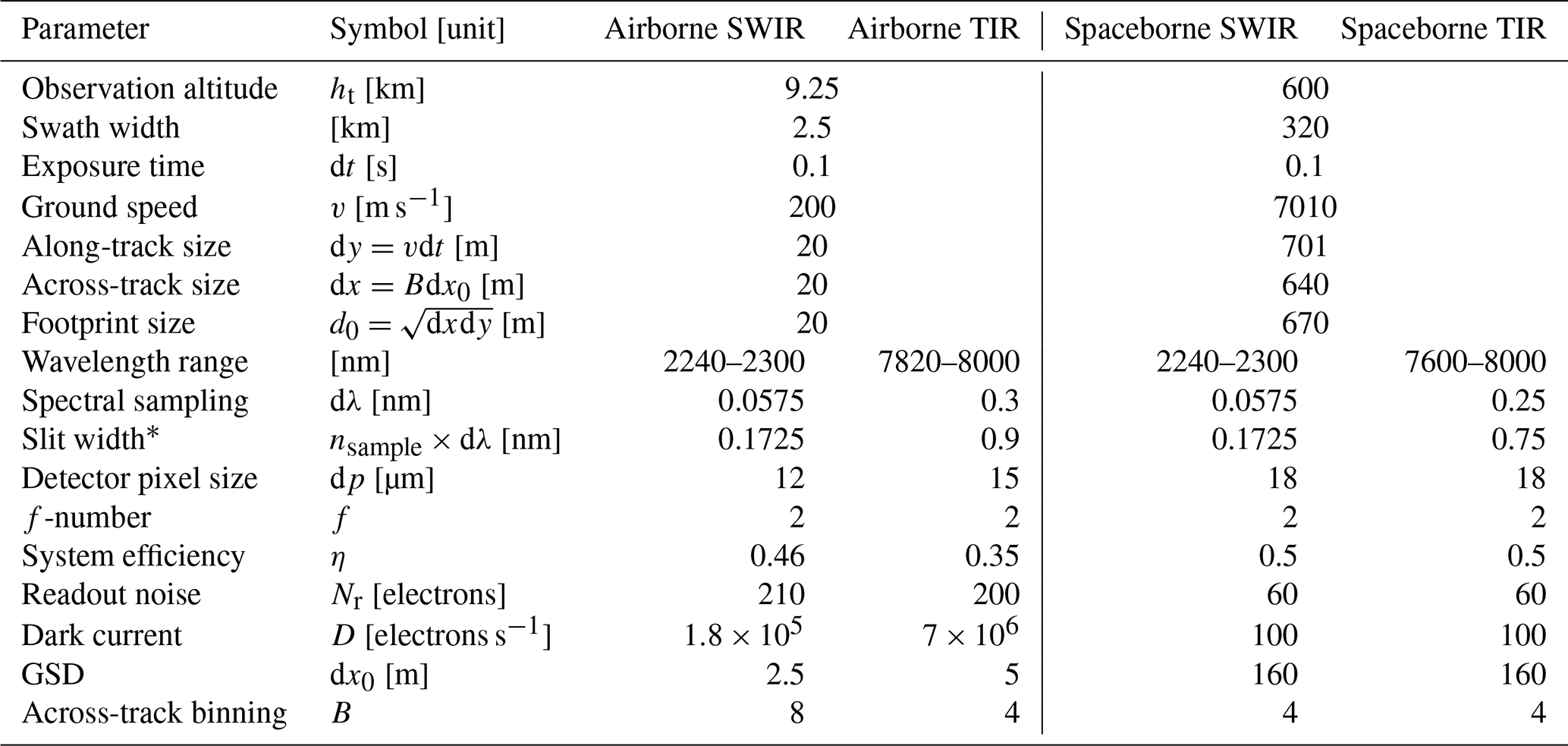
^∗ FWHM of Gaussian ISRF.

Due to limited space in the target aircraft, we choose smaller focal plane arrays (FPA) for the airborne instrument, which contain 1280×1024 pixels for the SWIR spectrometer and 640×512 pixels for the TIR spectrometer. The FPA dimension for the spaceborne instrument is 2048×2048 pixels for both bands. Due to the substantially smaller TIR focal plane array assumed for the airborne instrument relative to the spaceborne, a narrower TIR wavelength range is selected for the airborne case while maintaining the desired spectral performance. The along-track ground pixel size dy is determined by the ground speed of the platform v and the exposure time dt as dy=vdt. The swath width for the airborne instrument is about 2.5 km at a representative aircraft altitude of 9.25 km, and for the spaceborne instrument, about 320 km at an orbit height of 600 km. The native across-track ground pixel size, or ground sampling distance (GSD, denoted as dx₀), reflects how the swath is sampled by the spatial dimension of the FPA, which at maximum contains 1024 SWIR and 512 TIR pixels for the airborne instrument and 2048 pixels for the spaceborne instrument. To collocate the footprints of two bands and make them square-like, the native across-track pixels are binned by a factor B, such that the final across-track ground pixel size dx is

$$\begin{array}{}\text{(9)}& \mathrm{d}x=B\mathrm{d}{x}_{\mathrm{0}}.\end{array}$$

The combination of SWIR and TIR spectra associated with a common ground footprint with dimension dx×dy is referred to as a “sounding” of N₂O. For further analysis of the detectability of $X_{{\mathrm{N}}_{\mathrm{2}}\mathrm{O}}$ variability, it is helpful to define a footprint size d₀ for an N₂O sounding as the edge size of a square having the same area of the ground footprint:

$$\begin{array}{}\text{(10)}& d_{\mathrm{0}}=\sqrt{\mathrm{d}x\mathrm{d}y}.\end{array}$$

The spectral error covariance matrix (S_o) is assumed to be diagonal; in other words, the noise of individual detector pixels follows independent Gaussian distributions. The standard deviation of spectral error is calculated by multiplying each single-channel radiance r with SNR:

$$\begin{array}{}\text{(11)}& \mathrm{SNR}={\displaystyle \frac{S}{N}},\end{array}$$

where the signal S and noise N are measured by number of electrons. The signal is computed as

$$\begin{array}{}\text{(12)}& S={\displaystyle \frac{\mathit{\pi }}{\mathrm{4}}}\cdot r\cdot {\displaystyle \frac{\mathrm{d}{p}^{\mathrm{2}}}{f^{\mathrm{2}}}}\cdot n_{\mathrm{sample}}\cdot \mathrm{d}\mathit{\lambda }\cdot \mathrm{d}t\cdot \mathit{\eta },\end{array}$$

where r is the observed radiance at a specific wavelength (photons s⁻¹ cm⁻² nm⁻¹ sr⁻¹), dp is detector pixel size, f is f-number, n_sample is slit width measured as the ratio between the full width at half maximum of the instrument spectral response function (ISRF) and the spectral sampling interval, dλ, dt is exposure time, and η is system efficiency. All parameters except the radiance are listed in Table 1. The total noise per exposure is computed as the quadrature sum of readout noise (N_r) and shot noise, the latter having contributions from both the signal and the cumulative dark current (D) over the exposure time. Considering the across-track binning factor B, the noise for each sounding is

$$\begin{array}{}\text{(13)}& N=\sqrt{{\displaystyle \frac{S+D\mathrm{d}t+N_{\mathrm{r}}^{\mathrm{2}}}{B}}}.\end{array}$$

Figure 5 Top row shows simulated radiance spectra at the spectral ranges and resolutions of the spaceborne instrument, and bottom row shows corresponding signal-to-noise ratio (SNR). The left column shows the SWIR band (2240–2300 nm) with spectral resolution of 0.1725 nm, and the right column shows the TIR band (7600–8000 nm) with spectral resolution of 0.75 nm. In the top panels, the black curves represent simulated radiance with N₂O abundance set to zero, highlighting the absorption features attributable to N₂O. Radiance is expressed in units of photons s⁻¹ cm⁻² nm⁻¹ sr⁻¹. SWIR band shows weaker N₂O line strengths while the TIR band exhibits stronger absorption features and higher SNR due to strong signals.

Figure 5 (top row) shows the simulated radiance spectra of a daytime clear-sky summertime sounding selected from the CrIS ensemble over the US Midwest, at the spectral ranges and resolutions of the spaceborne instrument, with and without N₂O, using the radiative transfer model detailed in Sect. 3.1.4. The simulation assumes a solar zenith angle (SZA) of 30°, nadir viewing geometry, representative SWIR grass surface albedo of 0.159, TIR surface emissivity of 0.98, surface temperature of 307.3 K and thermal contrast of 4.6 K from the selected CrIS sounding. The spectral resolutions of the simulated spectra are 0.1725 nm for the SWIR band and 0.75 nm for the TIR band, corresponding to three times the spectral sampling intervals. In the SWIR band, differences with and without N₂O are small, owing to weak absorption lines, whereas the TIR N₂O features are much more prominent. The other spectral lines are mostly due to CH₄ and H₂O absorption with minor contributions from solar Fraunhofer lines for the SWIR. Figure 5 (bottom row) shows the corresponding SNR estimates calculated using Eq. (11) for the spaceborne instrument. The SNR for the SWIR band is significantly lower than that for the TIR due to lower radiance levels and finer spectral sampling. The SNR for the airborne instrument (not shown) appears similar but is slightly lower due to higher readout noise.

3.1.4 Radiative transfer simulation

For radiative transfer, this study leverages the VLIDORT radiative transfer model (Spurr, 2006), a discrete-ordinate multiple scattering code for a stratified multi-layer atmosphere. The great advantage for the present N₂O application is VLIDORT's ability to generate not only radiances (in scalar mode without polarization) or (for polarized light calculations) Stokes 3-vectors, but also any group of analytically-calculated Jacobians with respect to any atmospheric profile variable (temperature and trace gas mixing ratios) and any surface quantity (e.g., albedo, temperature, and emissivity).

The SPLAT environment compiles atmospheric meteorological and constituent profiles, along with reference datasets to generate the linearized inputs required by VLIDORT to simulate both radiance and analytically derived Jacobian with respect to atmospheric state variables. For gases, the input absorption cross sections are based on look-up tables derived from HITRAN 2020 (Gordon et al., 2022), while aerosol optical properties are represented using Mie and T-matrix calculation. For more on these setups and specific use on MethaneAIR retrieval, see Spurr and Christi (2014) and Chan Miller et al. (2024).

Although more widely used in radiative transfer of solar radiations (e.g., Liu et al., 2010; O'Dell et al., 2012), VLIDORT can operate in both solar and thermal regimes and has been used in joint ultraviolet-TIR ozone retrieval from separate instruments (Cuesta et al., 2013). In the thermal regime, VLIDORT's radiative transfer is driven by blackbody thermal emission, treated in the atmosphere as a piecewise-continuous linear function of layer optical thickness. VLIDORT ingests a set of Planck functions, specified for the atmosphere at all layer boundaries, and again at the surface. Thermal emission is unpolarized and is assumed isotropic. The Planck functions at layer boundaries are linearized in order to determine temperature-profile Jacobian contributions additional to those arising from the temperature dependencies in the optical thicknesses (Spurr and Christi, 2019). This study marks the first application of the SPLAT-VLIDORT framework on the joint solar and thermal radiative transfer of the same instrument. All radiative transfer simulations are performed on a 19-layer pressure grid extending from the surface to the top of atmosphere. The simulations use a solar zenith angle of 30°, viewing zenith angle of 0° and assume clear-sky conditions using the SPLAT–VLIDORT radiative transfer model and HITRAN2020 spectroscopy. Surface emissivity from CrIS L2 product is used for TIR band and representative grass surface albedo from ASTER is used for SWIR band. The state vector include profiles of N₂O, CH₄, H₂O, and temperature, along with surface temperature.

Figure 6 Jacobians with respect to N₂O, CH₄, H₂O, and temperature profiles for SWIR (a, c, e, g) and TIR (b, d, f, h) bands respectively. Each panel shows the sensitivity of observed radiance to a unit perturbation in the corresponding state variable as a function of pressure and wavelength. Only altitudes up until 100 hPa are shown to emphasize the troposphere and lower stratosphere, where most N₂O variability occurs. The distinct vertical sensitivity patterns between SWIR and TIR bands highlight their complementary roles in N₂O remote sensing.

Figure 6 shows the Jacobians of the SWIR (left column) and TIR bands (right column) with respect to atmospheric N₂O, CH₄, H₂O, and temperature profiles simulated by SPLAT-VLIDORT using profiles from a representative CrIS sounding and HITRAN2020 spectroscopy. The simulation conditions are same as described for Fig. 5 in Sect. 3.1.3. These Jacobians are calculated using the 19-layer atmospheric pressure grid, convolved with the ISRF and sampled at the spectral intervals of the spaceborne instrument specified in Table 1. Each panel represents a matrix, quantifying the change in observed radiance due to a unit perturbation in the state variable at given pressure level and wavelength. For N₂O (Fig. 6a–b), the SWIR band exhibits weak absorption but relatively uniform sensitivity throughout the column, while the TIR band provides stronger sensitivity in the mid- and upper troposphere, but less near-surface response. This complementary behavior reinforces the benefit of combining SWIR and TIR observations for improved N₂O retrievals.

3.2 Detectability of $X_{{\mathrm{N}}_{\mathrm{2}}\mathrm{O}}$ variability at different spatial scales

When spatially aggregating $X_{{\mathrm{N}}_{\mathrm{2}}\mathrm{O}}$ observations, the measurement error component propagated linearly from detector noise decreases with the target length scale d. This relationship assumes that the detector noise between individual soundings is independent and uncorrelated.

$$\begin{array}{}\text{(14)}& {\mathit{\sigma }}_{X_{{\mathrm{N}}_{\mathrm{2}}\mathrm{O}}}\left(d\right)={\mathit{\sigma }}_{X_{{\mathrm{N}}_{\mathrm{2}}\mathrm{O}}}\left(d_{\mathrm{0}}\right){\displaystyle \frac{d_{\mathrm{0}}}{d}},\end{array}$$

where ${\mathit{\sigma }}_{X_{{\mathrm{N}}_{\mathrm{2}}\mathrm{O}}}\left(d_{\mathrm{0}}\right)$ is the native measurement error at sounding footprint size d₀, obtained from the linear sensitivity analysis (Sect. 3.1). At a length scale d≥d₀, it is meaningful to compare the aggregated measurement error ${\mathit{\sigma }}_{X_{{\mathrm{N}}_{\mathrm{2}}\mathrm{O}}}\left(d\right)$ with the real-world $X_{{\mathrm{N}}_{\mathrm{2}}\mathrm{O}}$ variability ${\mathit{\delta }}_{X_{{\mathrm{N}}_{\mathrm{2}}\mathrm{O}}}\left(d\right)$. With a known $X_{{\mathrm{N}}_{\mathrm{2}}\mathrm{O}}$ spatial distribution, its spatial variability can be quantified through a semivariogram (Metheron, 1963; Souri et al., 2022):

$$\begin{array}{}\text{(15)}& {\mathit{\delta }}_{X_{{\mathrm{N}}_{\mathrm{2}}\mathrm{O}}}\left(d\right)=\sqrt{{\displaystyle \frac{\mathrm{1}}{\mathrm{2}}}〈({\mathrm{\Delta }}_d{X}_{{\mathrm{N}}_{\mathrm{2}}\mathrm{O}}{)}^{\mathrm{2}}〉},\end{array}$$

where ${\mathit{\delta }}_{X_{{\mathrm{N}}_{\mathrm{2}}\mathrm{O}}}\left(d\right)$ is the standard deviation that represents variability at length scale d. Δ_d is an operator that differentiates all $X_{{\mathrm{N}}_{\mathrm{2}}\mathrm{O}}$ values separated by distances in a range of d±ε, where ε controls the granularity of the distance binning. The angular brackets 〈〉 average all point pairs within the specified bin.

In reality, spatially distributed $X_{{\mathrm{N}}_{\mathrm{2}}\mathrm{O}}$ measurements that can support semivariogram calculation are very rare. Nonetheless, we can approximate the semivariogram of $X_{{\mathrm{N}}_{\mathrm{2}}\mathrm{O}}$ using the semivariogram of in situ measured N₂O mixing ratio in the PBL:

$$\begin{array}{}\text{(16)}& {\mathrm{\Delta }}_d{X}_{{\mathrm{N}}_{\mathrm{2}}\mathrm{O}}={\displaystyle \frac{\mathrm{1}-\exp (-h_{\mathrm{b}}/H)}{\mathrm{1}-\exp (-h_{\mathrm{t}}/H)}}{\mathrm{\Delta }}_d{\mathit{\mu }}_{{\mathrm{N}}_{\mathrm{2}}\mathrm{O}},\end{array}$$

where h_b is PBL height, h_t is observation altitude determined by the instrument design parameters listed in Table 1 and H=7.5 km is the assumed atmospheric scale height. ${\mathrm{\Delta }}_d{\mathit{\mu }}_{{\mathrm{N}}_{\mathrm{2}}\mathrm{O}}$ is the spatial differentiation of PBL N₂O mixing ratio between observation pairs separated by distance d, where ${\mathit{\mu }}_{{\mathrm{N}}_{\mathrm{2}}\mathrm{O}}$ represents the in situ measurements collected along horizontal flight legs within the well-mixed PBL. Because h_t is significantly larger than h_b, the variability of $X_{{\mathrm{N}}_{\mathrm{2}}\mathrm{O}}$ is smaller than that of ${\mathit{\mu }}_{{\mathrm{N}}_{\mathrm{2}}\mathrm{O}}$. Equation (16) holds when the variability of $X_{{\mathrm{N}}_{\mathrm{2}}\mathrm{O}}$ is dominantly driven by the variability in the PBL, and the PBL N₂O mixing ratio is approximately uniform in the vertical direction. Combining Eqs. (15) and (16), we obtain:

$$\begin{array}{}\text{(17)}& {\mathit{\delta }}_{X_{{\mathrm{N}}_{\mathrm{2}}\mathrm{O}}}\left(d\right)={\displaystyle \frac{\mathrm{1}-\exp (-h_{\mathrm{b}}/H)}{\mathrm{1}-\exp (-h_{\mathrm{t}}/H)}}\sqrt{{\displaystyle \frac{\mathrm{1}}{\mathrm{2}}}〈({\mathrm{\Delta }}_d{\mathit{\mu }}_{{\mathrm{N}}_{\mathrm{2}}\mathrm{O}}{)}^{\mathrm{2}}〉}.\end{array}$$

Here, the semivariogram is directly calculated from extensively measured N₂O mixing ratios (${\mathit{\mu }}_{{\mathrm{N}}_{\mathrm{2}}\mathrm{O}}$) along horizontal flight legs within the well-mixed PBL during the MAIZE campaign, and the PBL height is inferred from collocated spiral profiles by identifying the sharp vertical transition of trace gases, temperature, and relative humidity between the well-mixed boundary layer and the free troposphere (Zhang et al., 2020). The $X_{{\mathrm{N}}_{\mathrm{2}}\mathrm{O}}$ variabilities calculated using Eq. (17) differ between the airborne and spaceborne instruments because they sample different portions of the atmospheric column due to their different observational height (h_t). The semivariograms are calculated for each flight from 0 to 50 km with 0.25 km bin width.

Since $X_{{\mathrm{N}}_{\mathrm{2}}\mathrm{O}}$ measurement error decreases with d (Eq. 14), and $X_{{\mathrm{N}}_{\mathrm{2}}\mathrm{O}}$ variability typically increases with d (Eq. 17), a critical spatial scale for variability can be numerically solved from the following equation:

$$\begin{array}{}\text{(18)}& q\times {\mathit{\sigma }}_{X_{{\mathrm{N}}_{\mathrm{2}}\mathrm{O}}}\left(d^{\ast }\right)={\mathit{\delta }}_{X_{{\mathrm{N}}_{\mathrm{2}}\mathrm{O}}}\left(d^{\ast }\right),\end{array}$$

where q is a positive scalar. The solution d^∗(q) is the aggregated spatial scale beyond which $X_{{\mathrm{N}}_{\mathrm{2}}\mathrm{O}}$ variability exceeds q times the measurement error. q=1 means the variability equals the measurement error, and q=2 means the variability is twice the measurement error, which is typically assumed as the threshold of detectability (Jacob et al., 2016).

3.3 Detectability of N₂O emissions at different spatial scales

A complementary way of understanding N₂O detectability is to characterize the critical spatial scales of detectable N₂O emission sources. Here, we adopt the approach from Jacob et al. (2016) for CH₄ detectability. Similar to Sect. 3.2, we aim to determine a critical spatial scale for emission, $d^{+}(q,E)$, beyond which the $X_{{\mathrm{N}}_{\mathrm{2}}\mathrm{O}}$ enhancement due to emissions at value E is q times the measurement error.

Assuming a uniform emission flux E and wind speed U, the enhancement of N₂O column amount due to emission at aggregated spatial scale d is

$$\begin{array}{}\text{(19)}& \mathrm{\Delta }\mathrm{\Omega }={\displaystyle \frac{Ed}{U}}.\end{array}$$

The N₂O enhancement increases with emission intensity and accumulating distance and decreases with wind speed. We assume U=5 km h⁻¹ following Jacob et al. (2016). At the same length scale d, the measurement error of the observable column amount, σ_Ω, can be derived from Eq. (14) by converting $X_{{\mathrm{N}}_{\mathrm{2}}\mathrm{O}}$ to a column amount:

$$\begin{array}{}\text{(20)}& {\mathit{\sigma }}_{\mathrm{\Omega }}={\mathit{\sigma }}_{X_{{\mathrm{N}}_{\mathrm{2}}\mathrm{O}}}{\displaystyle \frac{p_{\mathrm{s}}\left(\mathrm{1}-\exp (-h_{\mathrm{t}}/H)\right)}{Mg}}{\displaystyle \frac{d_{\mathrm{0}}}{d}},\end{array}$$

where p_s is surface pressure assumed to be 1000 hPa, M is air molar weight, and g is gravity and H is the assumed atmospheric scale height. The single-sounding measurement error ${\mathit{\sigma }}_{X_{{\mathrm{N}}_{\mathrm{2}}\mathrm{O}}}$ (at d₀, notation dropped for simplicity), sounding footprint size d₀, and observation altitude h_t are inherent properties of the instrument. h_t is the only vertical parameter in this formulation and is used to determine the vertical extent of the atmospheric column observed by the instrument. Other parameters in Eqs. (19) and (20) can be held constant except emission E and aggregation length scale d. Then, the detectability metric q can be calculated by dividing Eqs. (19) and (20):

$$\begin{array}{}\text{(21)}& q(E,d)={\displaystyle \frac{\mathrm{\Delta }\mathrm{\Omega }}{{\mathit{\sigma }}_{\mathrm{\Omega }}}}={\displaystyle \frac{E{d}^{\mathrm{2}}Mg}{U{\mathit{\sigma }}_{X_{{\mathrm{N}}_{\mathrm{2}}\mathrm{O}}}{d}_{\mathrm{0}}{p}_{\mathrm{s}}\left(\mathrm{1}-\exp (-h_{\mathrm{t}}/H)\right)}}.\end{array}$$

Equation (21) indicates that q increases linearly with emission, E, and quadratically with length scale, d, consistent with the intuition that more intensive and expansive emission sources are easier to detect. Alternatively, we can fix q to a certain value, e.g., 1 or 2, and solve for the critical length scale for emission level E:

$$\begin{array}{}\text{(22)}& d^{+}(q,E)=\sqrt{{\displaystyle \frac{qU{\mathit{\sigma }}_{X_{{\mathrm{N}}_{\mathrm{2}}\mathrm{O}}}{d}_{\mathrm{0}}{p}_{\mathrm{s}}\left(\mathrm{1}-\exp (-h_{\mathrm{t}}/H)\right)}{EMg}}}.\end{array}$$

4 Results

This section presents the outcomes of the linear sensitivity analysis and detectability methods introduced in the Sect. 3. Section 4.1 presents the dependence of $X_{{\mathrm{N}}_{\mathrm{2}}\mathrm{O}}$ measurement error and vertical sensitivity on spectral bands, observing platform properties, and a priori constraint strength. Section 4.2 uses semivariogram-based analysis to quantify the critical spatial scales at which natural $X_{{\mathrm{N}}_{\mathrm{2}}\mathrm{O}}$ variability becomes distinguishable from random measurement error. Section 4.3 relates emission strength, $X_{{\mathrm{N}}_{\mathrm{2}}\mathrm{O}}$ measurement error, and $X_{{\mathrm{N}}_{\mathrm{2}}\mathrm{O}}$ enhancement, providing a quantitative assessment of the critical spatial scales at which surface N₂O emissions can be resolved by the proposed instruments.

4.1 $X_{{\mathrm{N}}_{\mathrm{2}}\mathrm{O}}$ measurement error and vertical sensitivity by airborne and spaceborne instruments

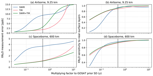
We evaluate the effectiveness of airborne and spaceborne instruments in retrieving $X_{{\mathrm{N}}_{\mathrm{2}}\mathrm{O}}$ by analyzing their measurement error and vertical sensitivity. The measurement error is calculated using Eq. (6) and vertical sensitivity is calculated using Eq. (8). Both metrics reflect the combined effect of observational constraint imposed by the instrument design and a priori constraint, as detailed in Sect. 3.1. Figure 7 illustrates the dependence of $X_{{\mathrm{N}}_{\mathrm{2}}\mathrm{O}}$ measurement error and near-surface sensitivity on the strength of a priori constraint for airborne and spaceborne instruments specified in Table 1 and compare results of three spectral settings; SWIR-only, TIR-only and joint SWIR–TIR setting. The near-surface sensitivity here is defined as the mean averaging kernel value of the lowest two atmospheric layers, representing the lowest ∼ 1 km of the atmosphere (corresponding pressure values are 962 and 901 hPa). In Fig. 7 the a priori constraint is adjusted by scaling the GOSAT/MethaneSAT-based N₂O prior standard deviation profile (see Fig. 4a) by a factor γ.

Figure 7 $X_{{\mathrm{N}}_{\mathrm{2}}\mathrm{O}}$ measurement error (left panels) and near-surface sensitivity quantified by the PBL mean of column averaging kernel (right panels) as a function of the a priori constraint strength (γ) applied to the N₂O prior standard deviation shown in Fig. 4a. Panels (a)–(b) correspond to the performance of the airborne instrument and panels (c)–(d) represent the performance of the spaceborne instrument. Each panel compares three spectral settings: SWIR-only (blue), TIR-only (pink), and combined SWIR–TIR (green) bands. Results are averaged over 100 CrIS soundings. The dual-band case achieves an optimal trade-off between near-surface sensitivity and $X_{{\mathrm{N}}_{\mathrm{2}}\mathrm{O}}$ measurement error at moderate strength of γ=0.5 by balancing the observational and a priori constraint for both remote sensing platforms.

The sensitivity analysis is performed using logarithmically spaced γ values between 0.03 and 10, spanning retrieval regimes from strong domination by the prior regularization (small γ) to those controlled primarily by the observation constraint (large γ). The applied γ only modulates N₂O a priori covariance matrix and does not affect the a priori covariance matrices of all other state vector elements. The results presented in Fig. 7 are the mean values calculated separately using the environmental conditions at 100 CrIS sounding locations shown in Fig. 1. These results correspond to single-shot observations at native instrument footprint size (d₀=20 m for airborne and d₀=0.7 km for spaceborne). Across the 100 selected CrIS soundings, the surface temperature ranges from 302.8 to 318.8 K (mean: 308.8 K), while the thermal contrast ranges from 2.8 to 12.3 K (mean: 6.6 K). Consistent across instruments and spectral settings, $X_{{\mathrm{N}}_{\mathrm{2}}\mathrm{O}}$ precision generally improves with tighter a priori constraint at small γ at the expense of degrading near-surface sensitivity.

For the airborne instrument (Fig. 7a–b), the $X_{{\mathrm{N}}_{\mathrm{2}}\mathrm{O}}$ measurement error shown in panel (a) reveals three distinct regimes. In the rightmost side with large γ, the retrieval is largely dependent on the amount of information provided by observations, with random detector noise dominating the error. In this regime, SWIR–TIR joint setting delivers the lowest measurement error as it combines information from two bands which increase the effective observational constraint. In contrast, the SWIR and TIR bands alone have fewer spectrum data points and thus provide weaker observation constraints than the joint band case, leading to larger errors. In a transition regime where γ is roughly 2–5, dual-band case briefly exhibit higher measurement errors than those from the SWIR or TIR bands alone, because the retrieval is less stabilized by the a priori constraint as compared to the single-band cases. In other words, SWIR-only and TIR-only cases begin to “feel” the a priori constraint earlier due to weaker observational constraints. As γ continues decreasing, all three cases become increasingly controlled by the a priori constraint, so the errors converge and the dual-band case falls between the SWIR-only and TIR-only cases. For the SWIR-only case, this transition to a prior-dominated regime is particularly abrupt, resulting in a rapid reduction in the $X_{{\mathrm{N}}_{\mathrm{2}}\mathrm{O}}$ measurement error that is synchronized with the simultaneous decrease in near-surface sensitivity. This behavior is also consistent with prior covariance tuning behavior reported for SWIR CH₄ retrievals in Chan Miller et al. (2024) and likely reflects the inherent differences between shortwave and longwave radiative transfer, including both the strength and vertical distribution of the N₂O Jacobians.

Figure 7b highlights the trade-off value of γ between measurement error and near-surface sensitivity. At a very large γ (rightmost side) the retrieval is primarily observation dominated, resulting in relatively strong TIR near-surface sensitivity due to the stronger TIR observational constraint. Under this regime, the SWIR-only retrieval exhibits the weakest near-surface sensitivity, while the joint SWIR–TIR retrieval benefits from complementary information from both bands and therefore shows the highest sensitivity. A very strong prior (leftmost side, small γ) suppresses the SWIR near-surface information which increases rapidly as the prior is relaxed and then reaches a plateau. A value of γ=0.5 (vertical black line) provides a balanced operating point because it sits on this plateau and SWIR near-surface sensitivity at this point is nearly saturated without entering the weak-prior regime where its value degrades quickly. This choice also keeps the dual-band case sensitive to observations in both bands, resulting in low measurement error while retaining sensitivity to the near-surface layers.

For the spaceborne instrument (Fig. 7c–d), the same qualitative order holds but the curves are less structured. $X_{{\mathrm{N}}_{\mathrm{2}}\mathrm{O}}$ measurement error (Fig. 7c) is overall lower than that from the airborne instrument largely due to the significantly wider TIR spectral range enabled by the spaceborne detector. The SWIR produces the largest measurement errors across all prior strengths. Both TIR-only and joint SWIR–TIR settings achieve comparable errors, but the integrated approach improves near-surface sensitivity relative to the TIR band alone (Fig. 7d). This added sensitivity is particularly beneficial given the inherently reduced surface sensitivity in satellite observations due to greater path lengths. We choose the same value of γ=0.5 for the spaceborne instrument because it provides a balanced operating point between observational and a priori constraint with retaining sensitivity to near-surface layers along with achieving low $X_{{\mathrm{N}}_{\mathrm{2}}\mathrm{O}}$ measurement error. At this selected operating point γ, single sounding $X_{{\mathrm{N}}_{\mathrm{2}}\mathrm{O}}$ measurement error for the joint SWIR–TIR retrieval spans the interval 2.8–3.8 ppb (mean: 3.2 ppb) for the airborne instrument at a footprint size of d₀=20 m, whereas that for the spaceborne instrument ranges 0.6–1.8 ppb (mean: 1.1 ppb) at d₀ of 0.7 km.

Figure 8 Column averaging kernels for N₂O retrievals using the SWIR-only (a, d), TIR-only (b, e), and joint SWIR–TIR (c, f) setting as a function of the a priori constraint strength (γ) applied to N₂O prior standard deviation shown in Fig. 4a. Panels (a)–(c) show results for the airborne instrument at 9.25 km observational altitude, and panels (d)–(f) show results for the spaceborne instrument at 600 km.

Figure 8 shows the vertical structure of the N₂O column averaging kernel for three spectral settings under different a priori strengths, illustrating how measurement information is spread throughout the observed atmospheric column. For the airborne instrument (Fig. 8a–c), the SWIR-only exhibits stronger sensitivity to the column with a discontinuity at the observation altitude of 9.25 km . This behavior follows the solar-backscattered nature of the viewing geometry where the incident sunlight samples the atmosphere only once above the aircraft, whereas the photons traverse the air mass twice (downward to the surface and then upward to the sensor) below the aircraft. In contrast, the TIR-only relies on thermal emissions and therefore show no sensitivity above the aircraft altitude, with its response confined to layers below 9.25 km. Within this region, TIR band shows an enhanced sensitivity in the layers just below the aircraft, which is plausibly related to the vertical weighting function in the retrieval. The joint SWIR–TIR setting alleviates this localized amplification and distributes the information more evenly by integrating complementary strengths of both bands.

For the spaceborne instrument (Fig. 8d–f), the overall vertical patterns are similar but smoother, because satellite geometry at orbital altitude avoids the discontinuity that appears in the case of airborne instrument. SWIR-only setting maintains strong column-wide sensitivity approaching near-unity kernel values for sufficiently relaxed a priori constraints. The TIR-only and the joint SWIR–TIR settings exhibit similar vertical response structures broadly, owing to the dominant contribution from the TIR band. Nevertheless, the inclusion of the SWIR band provides a visible improvement over the TIR-only case, particularly in enhancing sensitivity in the PBL, thereby highlighting the advantage of SWIR and TIR synergy for $X_{{\mathrm{N}}_{\mathrm{2}}\mathrm{O}}$ retrievals. For both instruments and all spectral settings, as the a priori constraint is relaxed (increasing γ), the averaging kernels start incorporating information from the observational constraint and shift from prior-dominated to measurement-informed.

4.2 Spatial scales of detectable $X_{{\mathrm{N}}_{\mathrm{2}}\mathrm{O}}$ variability

We determine the critical spatial scales for the airborne and spaceborne instruments at which $X_{{\mathrm{N}}_{\mathrm{2}}\mathrm{O}}$ variability becomes distinguishable from measurement error. Here, the observed spatial structure of $X_{{\mathrm{N}}_{\mathrm{2}}\mathrm{O}}$ variability is inferred from in situ PBL N₂O observations, and the instrument-specific $X_{{\mathrm{N}}_{\mathrm{2}}\mathrm{O}}$ measurement errors are estimated from the linear sensitivity analysis (see Sect. 3.2).

Figure 9 Semivariograms of PBL N₂O mixing ratios measured during the MAIZE campaign flights in 2022. Each colored line corresponds to a different flight date. The individual semivariograms reveal significant day-to-day variations likely due to heterogenetic nature of N₂O sources and localized meteorological conditions. The black line denotes the average semivariogram of all the flights, used as a representative model for quantifying critical spatial scales of detectable $X_{{\mathrm{N}}_{\mathrm{2}}\mathrm{O}}$ variability.

Figure 9 presents the semivariograms of PBL N₂O mixing ratios derived from eight MAIZE flights (i.e., $\frac{\mathrm{1}}{\mathrm{2}}\langle ({\mathrm{\Delta }}_d{\mathit{\mu }}_{{\mathrm{N}}_{\mathrm{2}}\mathrm{O}}{)}^{\mathrm{2}}\rangle$ in Eq. 17) along with their ensemble mean. Although the semivariance for all days generally increases with the separation distance, substantial variability is evident across individual flights. Several flights exhibit abrupt changes, which align with spatial intermittency in the PBL N₂O due to patchy sources and evolving boundary-layer conditions. The semivariogram sill, i.e., the maximum variance, also shows significant variation across flights, reflecting substantial differences in the overall intensity of heterogeneity. The extent of variability can also be attributed to meteorological conditions such as wind speed. Flights with stronger winds (e.g. 20220520, 20220521, 20220529, 20220530) show reduced semivariance as enhanced horizontal mixing diminishes spatial gradients, whereas flights with weaker winds (e.g. 20220518, 20220527) allow localized emission contrasts to persist, leading to higher semivariance. The ensemble-mean semivariogram, shown as the black line in Fig. 9, exhibits a smooth, steady rise and is utilized as a representative model of typical N₂O PBL variability for the subsequent detectability analysis.

Figure 10 $X_{{\mathrm{N}}_{\mathrm{2}}\mathrm{O}}$ variability and $X_{{\mathrm{N}}_{\mathrm{2}}\mathrm{O}}$ precision for airborne (blue) and spaceborne (black) instruments. Solid lines with circular markers show $X_{{\mathrm{N}}_{\mathrm{2}}\mathrm{O}}$ variability derived from the MAIZE flights, where the circular markers indicate the semivariogram distance bins separated by 0.25 km. Solid and dashed straight lines represent aggregated $X_{{\mathrm{N}}_{\mathrm{2}}\mathrm{O}}$ precision multiplied by detectability thresholds of q=1 and q=2 respectively. The critical spatial scales d^∗(q), where the atmospheric variability become q times the precision, are indicated by red stars in the figure.

Built on the MAIZE semivariograms, the observed PBL N₂O variability translates to expected $X_{{\mathrm{N}}_{\mathrm{2}}\mathrm{O}}$ variability through Eq. (17) and is then compared with $X_{{\mathrm{N}}_{\mathrm{2}}\mathrm{O}}$ measurement error for airborne and spaceborne instruments. Measurement error here refers to the single-sounding uncertainty at the native footprint size d₀, whereas the uncertainty after averaging independent soundings to the spatial aggregation scale d is referred to as $X_{{\mathrm{N}}_{\mathrm{2}}\mathrm{O}}$ precision. Figure 10 shows the trends of $X_{{\mathrm{N}}_{\mathrm{2}}\mathrm{O}}$ variability and $X_{{\mathrm{N}}_{\mathrm{2}}\mathrm{O}}$ precision as functions of the spatial aggregation scale (d). The two solid lines with circular markers in Fig. 10 represent the inferred $X_{{\mathrm{N}}_{\mathrm{2}}\mathrm{O}}$ variability for airborne (blue) and spaceborne (black) instruments, respectively. The circular markers represent the distance bins used in the semivariogram calculation. Although the same semivariogram is used in calculating the $X_{{\mathrm{N}}_{\mathrm{2}}\mathrm{O}}$ variability for both instruments, the results differ, as this variability depends on the observational altitude (h_t) of the instrument (see Eq. 17) and thus the relative weight of PBL variability in the observed atmospheric column. The higher h_t for the spaceborne instrument dilutes the boundary-layer heterogeneity more, yielding smaller $X_{{\mathrm{N}}_{\mathrm{2}}\mathrm{O}}$ variability as compared to that for airborne instrument at a given horizontal distance. The blue solid line in Fig. 10 corresponds to the aggregated precision ${\mathit{\sigma }}_{X_{{\mathrm{N}}_{\mathrm{2}}\mathrm{O}}}\left(d\right)$ of airborne instrument, and black solid line corresponds to that of spaceborne instrument, computed from single-sounding $X_{{\mathrm{N}}_{\mathrm{2}}\mathrm{O}}$ measurement error (${\mathit{\sigma }}_{X_{{\mathrm{N}}_{\mathrm{2}}\mathrm{O}}}\left(d_{\mathrm{0}}\right)=\mathrm{3.2}$ ppb for the airborne instrument and ${\mathit{\sigma }}_{X_{{\mathrm{N}}_{\mathrm{2}}\mathrm{O}}}\left(d_{\mathrm{0}}\right)=\mathrm{1.1}$ ppb for the spaceborne instrument) obtained in Sect. 4.1, using Eq. (14). Airborne and spaceborne precision lines do not overlap because ${\mathit{\sigma }}_{X_{{\mathrm{N}}_{\mathrm{2}}\mathrm{O}}}\left(d_{\mathrm{0}}\right)$ for airborne is larger (3.2 ppb) as compared to that for the spaceborne (1.1 ppb), and this quantity decreases quickly for the airborne instrument with the spatial averaging due to much smaller footprint size (d₀=20 m for airborne and d₀=0.7 km for spaceborne, see Table 1). As formulated in Eq. (14), the $X_{{\mathrm{N}}_{\mathrm{2}}\mathrm{O}}$ precision decreases log-linearly with d due to averaging of independent soundings, while the $X_{{\mathrm{N}}_{\mathrm{2}}\mathrm{O}}$ variability increases with d following the behavior shown in Fig. 9. The intersection points of these two quantities (marked with red stars in Fig. 10) define the critical spatial scale d^∗(q), at which atmospheric variability is q times the measurement error, as defined in Eq. (18). The dashed lines represent a more conservative detectability requirement by plotting $q\times {\mathit{\sigma }}_{X_{{\mathrm{N}}_{\mathrm{2}}\mathrm{O}}}\left(d\right)$ with a commonly used criterion of q=2. The corresponding intersection points locate the spatial scales where $X_{{\mathrm{N}}_{\mathrm{2}}\mathrm{O}}$ variability is twice the $X_{{\mathrm{N}}_{\mathrm{2}}\mathrm{O}}$ precision. For q=2, the critical spatial scale ($d^{\ast }(q=\mathrm{2})$) is approximately 2.5 km for the airborne and 22 km for the spaceborne instrument. This reflects how $X_{{\mathrm{N}}_{\mathrm{2}}\mathrm{O}}$ variability can be resolved from measurement noise under typical conditions observed during MAIZE.

4.3 Spatial scales of detectable N₂O emissions

In Sect. 4.2, the critical spatial scales for variability are inferred by comparing $X_{{\mathrm{N}}_{\mathrm{2}}\mathrm{O}}$ precision against $X_{{\mathrm{N}}_{\mathrm{2}}\mathrm{O}}$ variability that implicitly reflects the influence of surface emissions, but this variability does not provide a quantitative mapping between N₂O emission strength and $X_{{\mathrm{N}}_{\mathrm{2}}\mathrm{O}}$ enhancements. Here, we make that connection explicit by modeling expected $X_{{\mathrm{N}}_{\mathrm{2}}\mathrm{O}}$ enhancement resulting from a uniform emission strength E and comparing it to the corresponding $X_{{\mathrm{N}}_{\mathrm{2}}\mathrm{O}}$ precision at matching spatial scales. We then quantify the emissions detectability using the q(E,d) metric, introduced in Sect. 3.3. Here q(E,d) is a continuous variable, defined as the ratio of emission-induced enhancement in $X_{{\mathrm{N}}_{\mathrm{2}}\mathrm{O}}$ to the aggregated measurement error at spatial aggregation scale d (Eq. 21). Figure 11 shows q(E,d) as a function of emission strength (E) and spatial aggregation scale (d) as in Eq. (21) for the airborne (panel a) and spaceborne (panel b) instruments. Consistent across the instruments, detectability increases linearly with E and quadratically with d, implying that stronger sources can be detected at much finer scales while weaker emissions require substantial spatial aggregation to achieve the same level of confidence q.

Figure 11 Detectability metric q(E,d) as a function of emission strength (E) and spatial aggregation scale (d) for the (a) airborne and (b) spaceborne instruments. White regions indicate values below the minimum detectability threshold displayed in the plot ($q<{\mathrm{2}}^{-\mathrm{8}}$). Solid black contours indicate q=1 and q=2, where the $X_{{\mathrm{N}}_{\mathrm{2}}\mathrm{O}}$ enhancements due to emission E are equal to and twice the aggregated measurement error at d, respectively. Instrument-specific measurement errors at d₀ are taken from linear sensitivity analysis. Stronger emissions can be resolved from noise at lower spatial scales while weaker emissions require more spatial aggregation.

White regions in Fig. 11 correspond to the detectability values below the minimum plotted contour level ($q<{\mathrm{2}}^{-\mathrm{8}}$). The black contour lines in Fig. 11 indicate the solutions of Eq. (21) for q=1 and q=2; these provide a convenient way to read off the level of spatial aggregation needed to achieve a chosen detectability for a given emission strength. Here, q=1 means that an emission-induced enhancement is equal to the aggregated precision and q=2 indicates $X_{{\mathrm{N}}_{\mathrm{2}}\mathrm{O}}$ enhancement becomes twice the aggregated precision at a given spatial aggregation scale d. Using a representative uniform emissions of 5 nmol m⁻² s⁻¹, consistent with the mean value of all nodes from 21–24 May in Fig. 3b, Fig. 11 implies critical spatial scale d⁺ is ∼2.1 km for the airborne instrument at q=1 and ∼2.9 km at q=2. For the spaceborne instrument, the corresponding values are substantially larger with d⁺ ∼8.4 km at q=1 and ∼12 km at q=2. For a higher uniform emissions of 10 nmol m⁻² s⁻¹, the d⁺ reduces to 1.5 km at q=1 and 2.1 km at q=2 for the airborne instrument, and the corresponding values decreases to 5.9 km (q=1) and 8.5 km (q=2) for the spaceborne instrument. d⁺ values are different for airborne and spaceborne instruments as it is dependent on instrument properties such as footprint size (d₀), observational altitude (h_t) and single-sounding measurement error (${\mathit{\sigma }}_{X_{{\mathrm{N}}_{\mathrm{2}}\mathrm{O}}}\left(d_{\mathrm{0}}\right)$). Overall, weaker emissions require larger-scale spatial aggregation to achieve a certain detectability level for both instruments.

4.4 Critical spatial scales of N₂O detection estimated using different approaches

This section provides a combined view of critical spatial scales reported as d^∗ and d⁺ in Sect. 4.2 and 4.3, respectively. Table 2 summarizes these scales for the airborne and spaceborne instruments at two detectability levels, q=1 and q=2, illustrating how the required aggregation scale depends on detectability threshold and the approaches to estimate $X_{{\mathrm{N}}_{\mathrm{2}}\mathrm{O}}$ variability. In all cases, the airborne instrument consistently achieves smaller critical spatial scales as compared to spaceborne instrument. Although the airborne single-sounding error is larger, its much finer footprint size d₀ of 20 m allows more rapid reduction of random error with aggregation length scale d and detectability is achieved quickly under favorable conditions. In contrast, the spaceborne instrument with footprint size d₀ of 0.7 km, generally requires aggregation over several kilometers to reach the same detectability threshold, emphasizing that its strength lies in detecting broader regional patterns rather than localized enhancements.

Table 2 Critical spatial scales at which $X_{{\mathrm{N}}_{\mathrm{2}}\mathrm{O}}$ signals become q times the aggregated measurement error for airborne and spaceborne instruments. Value are reported for q=1 and q=2.

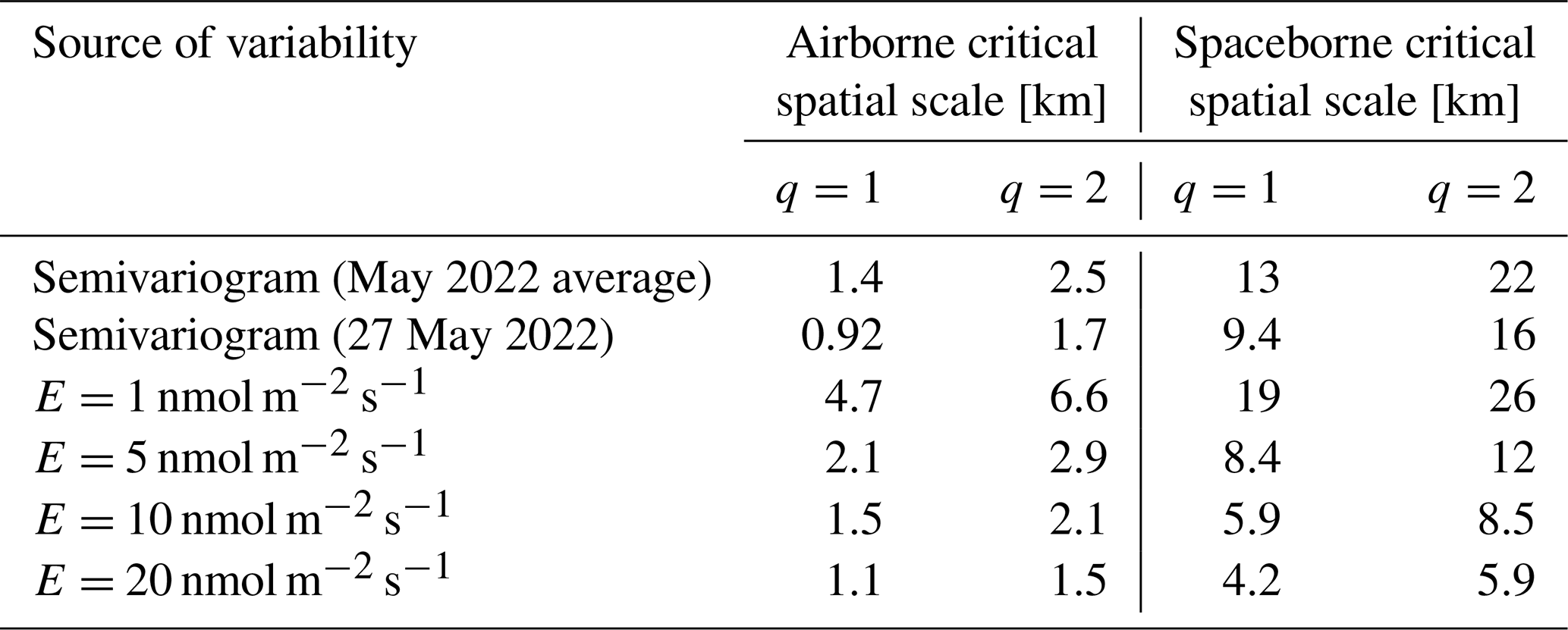
For the variability-driven estimates, the choice of semivariogram primarily controls the inferred critical spatial scales. Using the mean semivariogram of all 8 flights conducted in May 2022 yields more conservative critical spatial scales than using the semivariogram of highest-variability flight (27 May 2022), which represents a more favorable scenario associated with relatively weak wind and reduced atmospheric mixing conditions. When the $X_{{\mathrm{N}}_{\mathrm{2}}\mathrm{O}}$ variability is twice the $X_{{\mathrm{N}}_{\mathrm{2}}\mathrm{O}}$ precision, d^∗ reduces from 2.5 to 1.7 km for the airborne instrument and from 22 to 16 km for the spaceborne instrument when switching from the mean semivariogram to the high-variability semivariogram. For the emission-driven cases, the critical spatial scales d⁺ are reported for uniform emissions of E=1, 5, 10 and 20 nmol m⁻² s⁻¹ in Table 2. As anticipated, d⁺ decreases systematically with increasing uniform emission strength. For instance, increasing E from 1 to 20 nmol m⁻² s⁻¹, reduces the $d^{+}(\mathrm{2},E)$ from 6.6 to about 1.5 km for the airborne, and from 26 to around 5.9 km for the spaceborne instrument. Together, the variability- and emission-driven results bracket the spatial scales over which $X_{{\mathrm{N}}_{\mathrm{2}}\mathrm{O}}$ signals are expected to become detectable under typical MAIZE-like boundary-layer variability and plausible agricultural emissions.

5 Summary and Conclusions

This study develops a practical and physically grounded framework to evaluate the capability of remote sensing instruments to detect atmospheric N₂O variability and column enhancements. To achieve this purpose, we expand the capacity of the SPLAT-VLIDORT radiative transfer model to jointly simulate solar-reflected (SWIR) and thermal-emitted (TIR) spectra within a unified framework. This framework provides a quantitative basis for assessing the combined observation from the SWIR and TIR bands under a priori regularization, with a particular emphasis on the trade-off between random measurement error and sensitivity to near-surface variability. A central consideration here is the use of $X_{{\mathrm{N}}_{\mathrm{2}}\mathrm{O}}$ measurement error, which is derived by linear propagation of Gaussian instrument noise. Although this represents only one component of the total error budget, it provides a lower bound on the achievable single-sounding error and therefore a first-order constraint for any N₂O-focused mission. Also, in the error budget, measurement error is the only component that decreases predictably with spatial averaging of independent soundings, with the error scaling approximately as $\mathrm{1}/\sqrt{N}$, where N is the number of independent soundings being aggregated. This relationship provides a direct link between single-sounding error and spatial aggregation scales required for resolving $X_{{\mathrm{N}}_{\mathrm{2}}\mathrm{O}}$ enhancements above the noise.

The linear sensitivity analysis further shows that the a priori constraint plays a decisive role in balancing observational and a priori contributions to the vertical distribution of information. A key methodological direction for future refinement is to move beyond a scaled prior covariance toward an ensemble covariance that will allow the regularization to be informed by physically plausible variability rather than an assumed scaling. Within the current setup, the joint SWIR–TIR setting balances the observational and a priori information contributions at a moderate prior strength by scaling N₂O prior standand deviation by 0.5. At this prior strength, dual-band case yields single-sounding measurement error of 3.2 ppb for the airborne instrument with 20 m footprint size and 1.1 ppb for the spaceborne instrument with 0.7 km footprint size, while preserving sensitivity to the near-surface layers.

An additional factor that could influence the performance is the presence of atmospheric aerosols. Aerosol scattering in the SWIR band modifies the photon path length and if not handled properly can introduce biases in the retrieved $X_{{\mathrm{N}}_{\mathrm{2}}\mathrm{O}}$. Although, SPLAT–VLIDORT framework can incorporate aerosol optical properties, the scope of this study is limited to clear-sky condition. Future work should incorporate the influence of aerosol properties on $X_{{\mathrm{N}}_{\mathrm{2}}\mathrm{O}}$ accuracy, and how the SWIR and TIR bands can be synergized to account for aerosol influences.

The instrument precision alone does not fix the detectability; rather, it is determined by how the instrument precision interacts with real-world $X_{{\mathrm{N}}_{\mathrm{2}}\mathrm{O}}$ variability. We therefore estimate the critical spatial scales of detection using two data-informed approaches that address different aspects of this problem and rely on distinct simplifying assumptions. First, the semivariogram-based analysis provides an empirical constraint on how $X_{{\mathrm{N}}_{\mathrm{2}}\mathrm{O}}$ variability grows with separation distance under realistic agricultural conditions sampled during the MAIZE campaign. Its main assumption is that $X_{{\mathrm{N}}_{\mathrm{2}}\mathrm{O}}$ variability is dominated by PBL variability and the PBL N₂O mixing ratio is approximately uniform in the vertical direction (Eqs. 16–17). Second, the emission-based detectability metric q(E,d) links emission strength and spatial aggregation scales to expected $X_{{\mathrm{N}}_{\mathrm{2}}\mathrm{O}}$ enhancements using an assumed wind speed of 5 km h⁻¹. The emission strengths considered are informed by the autochamber data shown in Fig. 3. These approaches are intended to provide first-order constraints rather than universal thresholds, and the inferred critical spatial scales should be interpreted as conditional on variability, emission strength, meteorology, and the chosen aggregation strategy.

Under MAIZE-like conditions, semivariogram-based analysis indicates that natural $X_{{\mathrm{N}}_{\mathrm{2}}\mathrm{O}}$ variability exceeds instrument precision at critical spatial scales of approximately 1–3 km for airborne and 10–23 km for spaceborne observations. Episodic agricultural emissions of 5 nmol m⁻² s⁻¹ require aggregation of measurement error to spatial scales of roughly 2–3 km for airborne and ≈ 8–12 km for spaceborne instrument to achieve required level of detection confidence. Together these results emphasize the complementary roles of airborne and spaceborne observing platforms. Airborne instruments are best suited for resolving fine-scale heterogeneity associated with episodic emissions, whereas spaceborne observations can detect subtle column enhancements through spatial averaging while maintaining regional coverage. Overall, the combined SWIR–TIR band concept for N₂O remote sensing introduced in this study addresses the longstanding limitations of SWIR and TIR bands alone, laying a foundation for future N₂O-focused missions by offering practical guidance for instrument design.