Experimental determination of the lidar ratio for cirrus and polar stratospheric clouds at Dome C, Antarctica, using a Young inversion

We present 3 years (2022–2024) of polarisation lidar observations of polar stratospheric clouds (PSCs) and tropospheric cirrus above Concordia Station (Dome C, Antarctica). Layer-mean lidar ratios (LR) at 532 nm are retrieved using the Young inversion method applied to an elastic backscatter and depolarisation (Rayleigh) lidar. The measurements are classified in the $(\mathrm{1}-\mathrm{1}/R,{\mathit{\delta }}_{\mathrm{T}})$ phase space, allowing us to separate supercooled ternary solution (STS), nitric-acid trihydrate (NAT) and ice PSC, as well as upper-tropospheric cirrus.

To quantify the impact of the Young assumptions, we analyse both the full set of cloud detections and a Young-optimized subset of clouds that satisfy stricter homogeneity conditions above and below the cloud layer. The comparison between these two datasets allows us to separate the effective climatological variability of lidar ratio values from those retrieved under idealised conditions that strictly satisfy the Young inversion assumptions. For PSCs, the full dataset yields optically weighted median LR values (25–75 percentiles) of 38 (31–52) sr for STS, 49 (37–67) sr for NAT, and 52 (41–66) sr for ice PSC. For cirrus, the median LR is 50 (33–52) sr. These values are consistent with microphysical expectations and with previous ground-based and spaceborne lidar studies.

The Young-optimized subset yields 38 (31–59) sr for STS, 59 (38–74) sr for NAT, 38 (32–38) sr for the few remaining ice PSC, and 40 (32–40) sr for cirrus although for this latter case the number of observations is not statistically significant. The subset thus provides a conservative methodological benchmark for conditions that most closely satisfy the Young inversion assumptions, while the full dataset captures the broader range of cloud variability.

The comparison between the full dataset and the Young-optimized subset shows that the retrieved LR statistics are not controlled only by particle type, but also by cloud structural complexity and mixing. In particular, ice PSC and some cirrus layers frequently violate the vertical homogeneity assumptions of the Young method, so that their layer-mean LR should be interpreted as an effective value representative of mixed or vertically structured clouds rather than as a pure microphysical signature.

These values provide a physically consistent reference for PSC and cirrus retrievals over Dome C and can be used in radiative-transfer modelling and satellite-lidar validation.

1 Introduction

Cirrus clouds in the troposphere and polar stratospheric clouds (PSCs) in Antarctica play a central role in the radiative budget, transport and dehydration processes, and, in the case of PSCs, the heterogeneous chemistry responsible for polar ozone depletion (Solomon, 1999; Peter and Grooß, 2012). Elastic backscatter lidar with polarization capability provides continuous vertical profiling of cloud backscatter and depolarization, allowing discrimination between ice, supercooled ternary solutions (STS), and nitric acid trihydrate (NAT) particles (Pitts et al., 2018; Hostetler et al., 2006). A key parameter controlling the conversion of attenuated backscatter into extinction is the lidar ratio (LR), which directly links the optical and microphysical properties of cloud particles. Accurate LR values are essential for retrieving cloud optical depth, quantifying radiative effects, and constraining particle phase and habit (Reichardt et al., 2004; Ansmann et al., 1992).

Ground-based and satellite Rayleigh lidar measurements do not provide independent constraints on backscattering and extinction simultaneously; consequently, such studies have often relied on fixed or aerosol- and cloud-type-dependent LR values. For PSCs, early modelling analyses suggested LR₅₃₂ in the range 40–70 sr at 532 nm, with lower values associated with liquid/STS layers and higher values for NAT- and ice-dominated clouds (Gobbi, 1995). In practice, several long-term PSC data sets have adopted constant LR of 40–50 sr for all PSC types or for specific categories: for example, Córdoba-Jabonero et al. (2013) used LR₅₃₂=40 sr in Arctic micropulse-lidar observations, while CALIPSO operational products assume fixed LR of order 50 sr for all PSC classes (Kim et al., 2018), while refined PSC-type based choices have also been implemented (Pitts et al., 2018). More recent case studies exploiting Raman or Rotational–Raman channels have started to retrieve LR directly, reporting values of LR₃₅₅=20–25 and LR₅₃₂=55–60 sr for spherical PSC observed over the European Arctic (Böckmann and Ritter, 2023), and confirming that ice and NAT PSC can reach LR well above 60 sr in mountain-wave events (Reichardt et al., 2004). Noel et al. (2009) reported low-to-medium lidar-ratio values, with LR₅₃₂=20–50 sr, consistent with type II PSCs.

A further complication is that background stratospheric aerosol itself can have LR comparable to that of PSC. Raman-lidar measurements at Antarctic and Arctic sites indicate LR₅₃₂ of ∼50–60 sr for volcanically enhanced sulfate aerosol (David et al., 2012; Achtert et al., 2013).

For cirrus, a similarly broad range of lidar ratio values has been reported. Ground-based and spaceborne retrieval algorithms often assume fixed LR₅₃₂ values of 25–30 sr (Josset et al., 2012; Kim et al., 2018), while direct measurements show site-dependent mean values ranging from ∼30 sr at mid-latitudes (Chen et al., 2002; Yorks et al., 2011) up to ∼40–45 sr in polar regions, with median cirrus LR₅₃₂ of 42±10 sr reported over Nyålesund (Nakoudi et al., 2021). Long-term lidar observations have further shown that such variability in cirrus optical properties has direct implications for radiative forcing estimates, with constrained lidar-ratio ranges commonly adopted to ensure physically consistent extinction retrievals (Lolli et al., 2026).

This spread reflects changes in particle shape, size and habit related to temperature, ventilation and water vapour availability, and, in the case of PSC, temperature-dependent transitions between STS, NAT and ice (Luo et al., 2003; Höpfner et al., 2006).

Such variability introduces uncertainty in extinction retrievals and hence in the interpretation of PSC and cirrus optical, microphysical and radiative properties when a single lidar ratio value is assumed to be representative of all cloud conditions. This uncertainty is further enhanced in mixed-phase polar stratospheric clouds, where the coexistence of STS, NAT and ice particles with different shapes and size distributions leads to complex and non-linear optical scattering behaviour (Cairo et al., 2023). A physically constrained alternative is the Young inversion method (Young, 1995; Young and Vaughan, 2009), which estimates an effective layer-mean LR directly from the measured elastic-lidar profile by imposing top-bottom consistency of the particle backscatter ratio after correction for cloud extinction. While this approach is routinely used in CALIPSO/CALIOP processing (Vaughan et al., 2004; Kim et al., 2018), long-term applications to ground-based polar lidar observations remain relatively limited, and the range of LR values obtained under strictly controlled Young conditions has not yet been fully characterised for PSCs and cirrus at Dome C. While previous Dome C studies have documented PSC occurrence and optical classification in the backscatter-depolarization phase space (Snels et al., 2021; Di Liberto et al., 2024), a multi-year, ground-based determination of layer-mean LR for the main PSC microphysical classes and tropospheric cirrus using a uniform Young-inversion framework has not yet been reported.

Dome C, on the East Antarctic Plateau, provides particularly favourable conditions for this analysis because its extremely low winter temperatures, stable meteorological conditions, and long polar night allow extended and continuous observations of PSCs and upper-tropospheric cirrus.

In this work we present a comprehensive determination of the lidar ratio for cirrus and for all PSC classes observed at Dome C using an implementation of the Young inversion applied to multi-year (2022–2024) 532 nm polarization lidar profiles. The processing chain includes crosstalk correction, molecular and aerosol extinction removal, cloud detection, and iterative cloud LR retrieval. A dedicated statistical module aggregates all retrieved cloud points and produces optically weighted distributions in backscatter–depolarization space, enabling the robust separation of STS, NAT, ice PSCs and cirrus. In this framework, the distinction between PSCs and cirrus clouds is performed using the altitude of the climatological tropopause as a reference: cloud points above this level are classified as PSCs, whereas those below are identified as cirrus. The resulting dataset represents the first unified ground-based LR climatology for polar clouds at Dome C, providing new observational constraints for lidar data processing, cloud radiative studies and for the evaluation of microphysical and chemical models in Antarctic conditions.

From a methodological perspective, this study explicitly distinguishes between lidar-ratio statistics derived from the full population of detected cloud layers and those obtained from a subset satisfying stricter Young homogeneity conditions. The former captures the full microphysical and dynamical variability of polar clouds, while the latter provides a physically conservative benchmark representative of vertically uniform layers for which the Young inversion assumptions are most closely fulfilled.

2 Site and instrumentation

2.1 Concordia Station (Dome C)

The observations analysed in this study were collected at Concordia Station (Dome C, 75°06^′ S, 123°23^′ E; 3233 m a.s.l.) on the East Antarctic plateau. The site is characterized by extremely low temperatures, particularly during the austral winter, stable meteorological conditions, and long polar night, with frequent occurrence of PSCs between June and September. The high altitude and the radiative cooling of the ice sheet strongly reduce tropospheric aerosol loadings, providing exceptionally clean background conditions for polarization lidar measurements. These conditions, combined with the long polar night, enable continuous operation of the instrument and extended time series suitable for cloud optical characterisation (Snels et al., 2021; Di Liberto et al., 2024). Over the June–October period, the dataset used here comprises 144 measurement days in 2022, 90 in 2023, and 112 in 2024.

2.2 Lidar system

The lidar system used in this work is a ground-based, single-wavelength, polarization-sensitive lidar operating at 532 nm. The lidar transmitter emits linearly polarised pulses at a repetition rate of 10 Hz. The receiver unit includes a Schmidt–Cassegrain telescope coupled to a two-channel polarization separation module, detecting the parallel and cross-polarized components (P_∥ and P_⟂) of the backscattered light. The effective vertical resolution of the processed profiles is 30–60 m, depending on the acquisition configuration. The basic acquisition time is 2 min; in the standard processing used for this study, 16 consecutive recordings are averaged, yielding an effective temporal resolution of 32 min. The lidar sounding can extend up to about 50 km under suitable signal-to-noise conditions. In the present analysis, however, the processed profiles are restricted to altitudes below 30 km, which fully covers the altitude range of the cirrus and PSC layers investigated in this study.

Raw signals are stored as photon-counting profiles, together with auxiliary molecular backscatter coefficients β_mol computed from co-located radiosonde measurements or standard atmospheric models. The lidar is routinely used for the detection and classification of cirrus clouds and PSCs at Dome C, and has been employed in previous coordinated studies with CALIPSO/CALIOP validations (Snels et al., 2021).

From the height-resolved measurements of parallel and cross-polarized backscatter signals, the volume backscatter coefficients β_∥(z) and β_⟂(z) can be retrieved, which contain contributions from both molecules and particles. Hence, volume depolarization ratios, and backscatter ratios, can be assessed. The volume depolarization ratio δ is defined as

$$\begin{array}{}\text{(1)}& \mathit{\delta }\left(z\right)={\displaystyle \frac{{\mathit{\beta }}_{⟂}\left(z\right)}{{\mathit{\beta }}_{\parallel }\left(z\right)}}={\displaystyle \frac{{\mathit{\beta }}_{⟂}^{\mathrm{mol}}\left(z\right)+{\mathit{\beta }}_{⟂}^{\mathrm{aer}}\left(z\right)}{{\mathit{\beta }}_{\parallel }^{\mathrm{mol}}\left(z\right)+{\mathit{\beta }}_{\parallel }^{\mathrm{aer}}\left(z\right)}}.\end{array}$$

The backscatter ratio is

$$\begin{array}{}\text{(2)}& R\left(z\right)={\displaystyle \frac{{\mathit{\beta }}_{\parallel }\left(z\right)+{\mathit{\beta }}_{⟂}\left(z\right)}{{\mathit{\beta }}_{\parallel }^{\mathrm{mol}}\left(z\right)+{\mathit{\beta }}_{⟂}^{\mathrm{mol}}\left(z\right)}}=\mathrm{1}+{\displaystyle \frac{{\mathit{\beta }}_{\mathrm{aer}}\left(z\right)}{{\mathit{\beta }}_{\mathrm{mol}}\left(z\right)}},\end{array}$$

where

$$\begin{array}{}\text{(3)}& {\mathit{\beta }}_{\mathrm{aer}}={\mathit{\beta }}_{\parallel }^{\mathrm{aer}}+{\mathit{\beta }}_{⟂}^{\mathrm{aer}},{\mathit{\beta }}_{\mathrm{mol}}={\mathit{\beta }}_{\parallel }^{\mathrm{mol}}+{\mathit{\beta }}_{⟂}^{\mathrm{mol}}.\end{array}$$

The aerosol (particle) and molecular depolarization ratios are defined as:

$$\begin{array}{}\text{(4)}& {\mathit{\delta }}_{\mathrm{A}}\left(z\right)={\displaystyle \frac{{\mathit{\beta }}_{⟂}^{\mathrm{aer}}\left(z\right)}{{\mathit{\beta }}_{\parallel }^{\mathrm{aer}}\left(z\right)}},{\mathit{\delta }}_{\mathrm{mol}}={\displaystyle \frac{{\mathit{\beta }}_{⟂}^{\mathrm{mol}}\left(z\right)}{{\mathit{\beta }}_{\parallel }^{\mathrm{mol}}\left(z\right)}}.\end{array}$$

Following Adachi et al. (2001) and Gimmestad (2008), we analyse the measurements in terms of the Total Particle Depolarization Ratio (δ_TA) and the Total Depolarization Ratio (δ_T). Gimmestad (2008) showed that adopting the δ_T definition provides a more coherent framework that harmonizes lidar depolarization analysis with radiative transfer theory, particle-scattering theory, and standard polarization measurement techniques.

The total volume depolarization ratio (Cairo et al., 1999) is

$$\begin{array}{}\text{(5)}& {\mathit{\delta }}_T\left(z\right)={\displaystyle \frac{{\mathit{\beta }}_{⟂}\left(z\right)}{{\mathit{\beta }}_{⟂}\left(z\right)+{\mathit{\beta }}_{\parallel }\left(z\right)}}={\displaystyle \frac{\mathit{\delta }\left(z\right)}{\mathit{\delta }\left(z\right)+\mathrm{1}}}.\end{array}$$

Similarly, the total particle depolarization is

$$\begin{array}{}\text{(6)}& {\mathit{\delta }}_{\mathrm{TA}}\left(z\right)={\displaystyle \frac{{\mathit{\beta }}_{⟂}^{\mathrm{aer}}\left(z\right)}{{\mathit{\beta }}_{\parallel }^{\mathrm{aer}}\left(z\right)}}={\displaystyle \frac{{\mathit{\delta }}_{\mathrm{mol}}+\left(R\right(z)-\mathrm{1}){\mathit{\delta }}_{\mathrm{A}}\left(z\right)}{R\left(z\right)}}.\end{array}$$

These quantities enable the retrieval of aerosol and cloud backscatter and the identification of microphysical regimes (STS, NAT, ice PSCs, cirrus) through combined analysis of backscatter enhancement and depolarization signatures. The subsequent processing described in Sects. 3 and 4 explains how these primary observations are retrieved

3 Data processing and methodology

The processing chain consists of a sequence of preprocessing, calibration, cloud-detection, inversion, and statistical-analysis steps. Because two distinct iterative procedures are used – one for cloud-boundary detection and one for the Young inversion itself – we summarize the full workflow below before describing each component in detail.

1. dark-count subtraction and range correction;

2. merging of tropospheric and stratospheric channels;

3. molecular normalization and depolarization calibration;

4. provisional extinction correction using LR =30 sr;

5. iterative cloud-boundary detection on R_fixed;

6. removal of the provisional correction;

7. Young inversion on the original attenuated profile;

8. selection of the Young-optimized subset using external homogeneity criteria;

9. optical weighting and statistical aggregation by cloud class.

Steps 1–3 correspond to lidar preprocessing and calibration. Steps 4–6 are used only to identify stable cloud boundaries and do not provide the final cloud optical properties. Step 7 is the Young inversion proper, while steps 8–9 are used for quality selection and statistical analysis. The individual components are described in the following subsections.

3.1 Lidar preprocessing and calibration

The raw lidar data consist of photon-counting profiles from the parallel (P_∥) and cross-polarized (P_⟂) channels acquired simultaneously by two partially overlapping acquisition chains at 60 m vertical resolution, a high-dynamic-range “tropospheric” channel and a more sensitive “stratospheric” channel each with its own telescope. Prior to inversion, the two channels are merged into a single continuous profile and processed through a sequence of calibration, crosstalk correction, molecular and aerosol extinction removal, cloud detection, and Young-type lidar ratio retrieval, as described below.

Dark counts are obtained from the uppermost part of the profile and subtracted from the raw photon counts. Profiles are optionally smoothed with a short moving-average filter over a 300 m window to suppress noise while preserving cloud boundaries. Statistical uncertainties are computed assuming Poisson counting statistics. The resulting uncertainty profiles are smoothed with a 300 m vertical moving-average window to reduce bin-to-bin noise and are stored as part of the final data product. The tropospheric channel provides a better linearity at low levels at the expense of a reduced signal-to-noise ratio, whereas the stratospheric channel ensures higher sensitivity in the upper atmosphere. The two channels are first background subtracted and range-corrected and normalized to their respective dynamic ranges. An altitude-dependent weighting function is applied over the overlap region between 8 and 12 km to produce a smooth transition between the tropospheric and stratospheric channels and to ensure continuity of the merged profile. A final consistency check compares the mean molecular signals in the overlap range. The resulting merged profiles serve as the base input for all subsequent steps.

Auxiliary molecular backscatter coefficients β_mol(z) are computed from co-located radiosonde measurements and, when unavailable, from standard atmospheric models. These are used to calculate the attenuated total backscatter and the corresponding attenuated backscatter ratio R_att. In addition, the ratio D of the cross- to parallel-channel signals ($P_{⟂}/P_{\parallel }$), proportional to the volume depolarization, is examined to identify altitude regions free of aerosol together with R_att.

A calibration interval is required to normalize the backscatter ratio and depolarization to their molecular reference values. A two-step automatic search scans the profile for candidate molecular regions where R_att≲1 and D≈δ_mol. Among these candidates, the segment minimizing the variance of both quantities is selected as the calibration interval. If no sufficiently stable region is found, a fixed calibration range is retrieved from a precompiled lookup table. This approach ensures robust and repeatable normalization across the multi-year dataset.

Accurate depolarization calibration is essential because the separation of STS, NAT, and ice PSCs relies directly on the measured polarization state of the backscattered signal. In the notation adopted here, consistently with the Concordia lidar calibration described by Di Liberto et al. (2024), $G=g_{\parallel }/g_{⟂}$ denotes the gain ratio between the parallel and cross-polarized detection channels, whereas CT denotes the cross-talk coefficient accounting for leakage from the parallel into the cross-polarized channel. The measured signals are corrected for optical and electronic cross-talk and for the gain ratio G, where $P_{\parallel ,⟂}\sim g_{\parallel ,⟂}{\mathit{\beta }}_{\parallel ,⟂}$. Following the molecular-consistency approach originally proposed in Di Liberto et al. (2024), the calibration relies on the fact that in purely molecular layers the ratio of the gain-normalized and cross-talk-corrected cross-polarized to the parallel backscatter must equal the known molecular depolarization δ_mol, which in our case is expected to be 0.007 (Behrendt and Nakamura, 2002).

In principle, both G and CT can be obtained through independent laboratory or on-site calibration procedures. When these measurements remain stable, the molecular-consistency requirement acts purely as a diagnostic check: any residual particulate depolarisation retrieved in the molecular reference region indicates imperfect calibration.

In practice, however, both parameters may undergo slow drifts due to detector ageing, thermal effects or optical realignment or change in the optical channels transmission and cross contamination. Because these drifts do not necessarily affect G and CT on the same timescale, it is often the case that one parameter (typically G) remains better constrained than the other. The inversion framework therefore offers a second operating mode: the more reliable parameter can be fixed, and the remaining one is adjusted so as to satisfy the molecular-consistency condition. This procedure does not “force’’ the cloud retrievals, but instead ensures that the instrument remains self-consistent in conditions where the true molecular depolarisation is known a priori.

After applying the selected correction scheme, the parallel and cross–polar signals are renormalised to obtain crosstalk-free profiles of attenuated backscatter ratio R_att and depolarisation δ, which form the basis for the subsequent Young inversion. The attenuated backscatter ratio is corrected for Rayleigh extinction using a molecular lidar ratio of 8.4 sr.

3.2 Cloud detection and boundary definition

To perform the Young inversion, cloud boundaries must be accurately identified, since the method requires a well-defined altitude interval over which particle extinction is retrieved. Direct detection of cloud base and cloud top from the attenuated backscatter ratio after molecular normalization but before particle-extinction correction R_att , can be unreliable because cloud extinction progressively attenuates the lidar signal and can distort the apparent vertical structure of (R_att). For this reason, an intermediate boundary-detection step is introduced.

First, a provisional particle-extinction retrieval is applied by assuming a fixed lidar ratio of 30 sr. This choice is not meant to reflect the true cloud optical properties. It is used only to partially compensate for the signal attenuation produced by cloud extinction, which can distort the vertical shape of R_att and obscure the gradients associated with cloud base and cloud top. The resulting provisionally corrected backscatter ratio is hereafter denoted as R_fixed. This is a provisional backscatter ratio obtained after applying the fixed LR of 30 sr and only used for cloud-boundary detection.

Cloud boundaries are then detected on R_fixed. The procedure is iterative: the boundaries obtained after the first pass are used to refine the provisional extinction retrieval, which further improves the localisation of cloud base and cloud top. The process is repeated until the cloud interval converges. Clouds are identified as contiguous altitude intervals where (R_fixed>1.15) and the geometrical thickness exceeds the minimum threshold adopted in the detection algorithm. Multiple fragments separated by fewer than 300 m are merged.

The resulting cloud intervals define the altitude regions where the Young inversion is applied. Once cloud base and cloud top are determined, the provisional correction based on LR =30 sr is discarded, and the Young inversion is applied to the original attenuated backscatter profile. A separate correction for background aerosol extinction is then applied outside cloud layers using a fixed aerosol LR of 70 sr, whereas inside cloud layers the LR is retrieved directly through the Young inversion.

3.3 Young inversion principle and implementation

The Young inversion is an elastic-lidar method used to estimate the layer-mean lidar ratio of a cloud when an independent Raman extinction measurement is not available. The input quantities are the attenuated backscatter ratio profile R_att, the molecular backscatter and extinction profiles, and the cloud base and top heights. The unknown quantity is the cloud lidar ratio, LR $={\mathit{\alpha }}_{\mathrm{p}}/{\mathit{\beta }}_{\mathrm{p}}$, which is assumed to be constant within the detected cloud layer.

The method relies on a top-bottom consistency condition. If the cloud is vertically homogeneous and is embedded in a horizontally and vertically uniform background, then the particle backscatter ratio immediately below and above the cloud should be the same after the attenuation produced by the cloud has been removed. For a trial value of LR, the particle extinction inside the cloud is estimated from the backscatter profile and used to correct R_att. This produces a corrected backscatter ratio, here denoted as R_cor. The optimal LR is then defined as the value that minimizes the absolute difference between the mean R_cor values in two cloud-free reference windows located below and above the cloud. In this study, the reference windows are 240 m thick and are offset by 180 m from the cloud boundaries. The offset and window thickness were chosen as a compromise between locality and statistical stability. The 180 m offset avoids the range bins immediately adjacent to the detected cloud boundaries, where uncertainties in cloud-edge location, smoothing, residual attenuation effects, or gradual cloud-background transitions may affect the signal. The 240 m window thickness provides enough vertical samples to compute a stable mean R_cor, while remaining close enough to the cloud to represent the local background conditions above and below the layer.

The retrieval is performed iteratively. For each trial LR, R_cor is first estimated inside the cloud, the corresponding particle-extinction correction is recomputed, and the top-bottom mismatch is evaluated again. This internal iteration is repeated until the corrected profile is self-consistent for that trial LR. The procedure is then repeated over the range of trial LR values, and the LR giving the smallest top-bottom mismatch is retained. The final retrieved quantity is therefore a single layer-mean LR for each detected cloud. It should be interpreted as an effective optical property of the whole cloud layer, rather than as a vertically resolved lidar-ratio profile.

3.4 Selection of clouds best suitable for unbiased Young inversion

The lidar ratio retrieved by the Young inversion relies on the assumption that the backscatter ratio R is identical immediately above and below a homogeneous cloud layer (Del Guasta, 1998). In real atmospheric conditions this requirement may be violated, especially for clouds exhibiting strong vertical gradients, embedded sub-layers, mixed-phase transitions or residual background aerosol. For this reason, we analyse the lidar ratio using two complementary approaches: (i) the full measurement set, providing the broadest and most complete representation of the observed variability, and (ii) a Young–optimised subset of clouds that satisfy stringent conditions and for which the inversion could be more physically robust.

The rationale for including the full data set is that it preserves the complete range of cloud structures encountered in real atmospheric conditions. Individual retrievals may be affected by local violations of the Young assumptions, but the resulting distribution provides an effective climatological description of the LR values that would be obtained in operational elastic-lidar analyses. The Young-optimized subset is then used as a complementary benchmark to evaluate how the statistics change when the assumptions of the method are more closely satisfied. Under this working hypothesis, the mean or median LR computed over the entire population would still yield a realistic representation of the climatological LR range for each cloud category, even if individual retrievals were affected by local errors. This approach preserves the full diversity of cloud structures observed above Dome C, including mesoscale temperature variation inducing ice PSCs, NAT/ice transitions, and multi-layer cirrus.

To obtain a complementary set of likely unbiased retrievals we constructed a Young–optimised subset by applying a sequence of more stringent homogeneity criteria designed to isolate clouds embedded in quasi-molecular conditions above and below. Each cloud is flanked by two control windows: one below the base and one above the top, each offset from the cloud boundaries by 180 m and extending for 600 m. Within each window we evaluate:

• a symmetry condition $S=\left|\frac{\langle R_{\mathrm{up}}\rangle -\langle R_{\mathrm{down}}\rangle }{\langle R_{\mathrm{up}}\rangle +\langle R_{\mathrm{down}}\rangle }\right|<\mathrm{0.10},$

• a homogeneity requirement $\mathrm{var}\left(R\right)/\mathrm{mean}\left(R\right)<\mathrm{0.10}$ in both windows,

• a smoothness criterion $|R_{i+\mathrm{1}}-R_i|<\mathrm{0.10}$ for all adjacent bins,

• a relative depolarisation constraint $d_{\mathrm{rel}}=\frac{|\langle {\mathit{\delta }}_{\mathrm{up}}\rangle -\langle {\mathit{\delta }}_{\mathrm{down}}\rangle |}{(\langle {\mathit{\delta }}_{\mathrm{up}}\rangle +\langle {\mathit{\delta }}_{\mathrm{down}}\rangle )/\mathrm{2}}<\mathrm{0.10}.$

Only clouds satisfying all tests are retained. The subset therefore consists of layers surrounded by aerosol-free, vertically uniform air, for which the Young inversion is expected to provide unbiased estimates of the lidar ratio. Presenting results from both data sets is thus essential: the full set captures the climatological LR variability across all microphysical regimes, whereas the Young–optimised subset provides a physically conservative benchmark of conditions for which the Young inversion is deemed more reliable.

The purpose of these criteria is not to optimise the retrieved lidar ratio toward specific numerical values, but to isolate cloud layers for which the Young inversion is expected to be most internally consistent. Although the numerical thresholds adopted here are necessarily empirical, their role is only to identify cloud layers for which the Young assumptions are more closely fulfilled. Moderate variations of these limits do not change the main effect of the filtering: the preferential retention of vertically simple layers and the exclusion of clouds embedded in highly variable backgrounds or characterized by strong internal inhomogeneity, for which a single layer-mean LR would not provide a fully self-consistent extinction correction.

Relaxing the Young-compatibility criteria would increase the number of retained layers, but at the cost of admitting cases with more variable background conditions or stronger internal cloud inhomogeneity. We therefore retained the stricter criteria in the final analysis. This choice favours methodological robustness over statistical representativeness for the Young-optimized subset, particularly for structurally complex classes such as ice PSC and some cirrus layers. The subset should therefore be interpreted as a conservative benchmark rather than as a statistically complete representation of each cloud class.

4 Statistical analysis

The dataset spans 144 measurement days in 2022, 90 in 2023, and 112 in 2024. However, the statistical analyses presented in this work are based on individual cloud layers identified within each measurement, rather than on the number of measurement days. Here, a cloud layer is defined as a contiguous altitude interval classified as cloudy within one lidar profile after the cloud-boundary detection procedure. Each detected cloud layer is assigned a single layer-mean LR by the Young inversion and therefore represents one independent LR retrieval. The larger number of points displayed in the two-dimensional phase-space figures corresponds instead to range-time samples within these cloud layers, weighted according to their aerosol backscatter contribution. These samples are used to describe the optical distribution of the cloud population in the ($\mathrm{1}-\mathrm{1}/R,{\mathit{\delta }}_T$) space, but they should not be interpreted as independent LR retrievals. Samples belonging to the same cloud layer are therefore temporally and vertically correlated and share the same retrieved layer-mean LR. They do not increase the effective number of independent observations, which remains the number of cloud layers reported in Table 1.

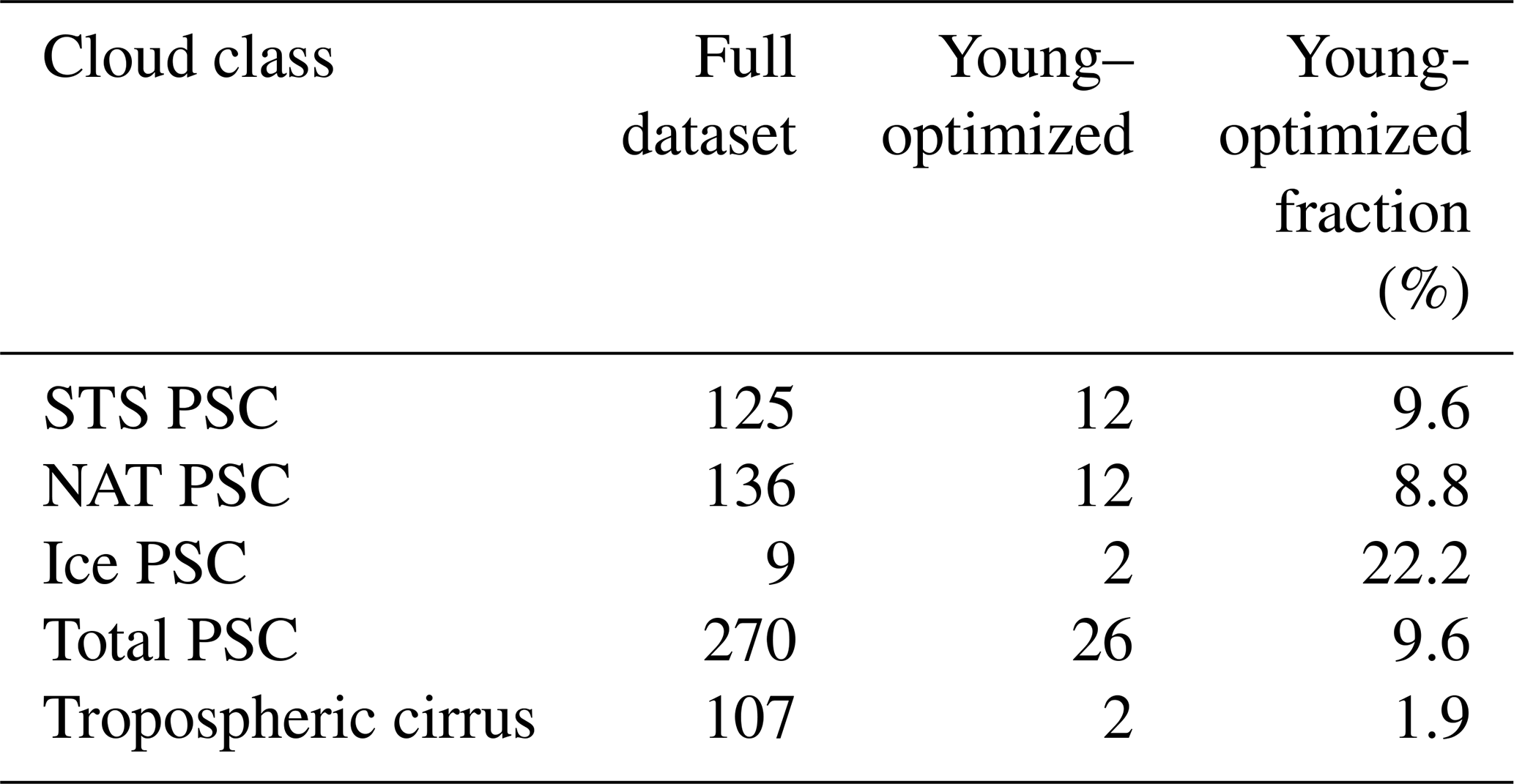
Table 1 Number of independent cloud layers contributing to each microphysical class in the full dataset and in the Young-optimized subset, together with the fraction retained by the Young-optimized criteria. A cloud layer is defined as one contiguous cloudy altitude interval detected in a single lidar profile. Each layer is assigned one layer-mean LR by the Young inversion. The number of cloud layers reported here should therefore not be confused with the larger number of range-time samples displayed in the two-dimensional phase-space figures. The Young-optimized fraction is an operational measure of compatibility with the Young inversion assumptions and should not be interpreted as a direct estimate of the fraction of internally homogeneous clouds.

The final Young-inverted products consist of vertically resolved profiles of lidar ratio (LR), backscatter ratio R_def, volume depolarization δ, particle depolarisation δ_A, aerosol backscatter coefficient β_aer in 60 m altitude bins, together with uncertainties, and diagnostic flags. For the statistical analysis we distinguish two cloud populations based on altitude: (i) tropospheric cirrus, defined as layers located below the climatological tropopause (12 km) (Snels et al., 2021) and (ii) polar stratospheric clouds (PSCs) located above this level. A sensitivity analysis was performed by varying the tropopause height by ± 2 km, which did not produce significant changes in the resulting LR statistics or in the classification of cloud types. The fixed 12 km tropopause is therefore used here as a reproducible operational separator between tropospheric cirrus and PSCs over the full 3-year dataset. Profile-by-profile tropopause estimates from radiosondes or model fields were not used for the main classification in order to avoid introducing an additional dependence on the temporal sampling and vertical resolution of the ancillary meteorological data. Nevertheless, the temperature profiles used to compute the molecular atmosphere provide important physical context for interpreting the retrieved LR values. For each cloud layer, temperature was therefore used diagnostically to relate the LR statistics to the expected thermodynamic regimes of STS, NAT, ice PSC and cirrus formation.

To separate the main PSC microphysical regimes we adopt simple, physically-based thresholds in R_def and δ_A. These criteria are chosen to isolate the “core” regions of each class while minimising overlap in transitional areas. The classification of PSC microphysical classes is based on physically motivated thresholds in backscatter ratio and depolarisation, consistent with previous analyses at Dome C and long-term lidar observations (Snels et al., 2021; Di Liberto et al., 2026; Serva et al., 2026).

• STS. $\mathrm{1.2}\le R_{\mathrm{def}}\le \mathrm{3}$ and δ_TA<0.05 occurring above the tropopause. This region corresponds to nearly spherical ternary-solution droplets, characterised by very low depolarisation and moderate backscatter enhancement.

• NAT. $\mathrm{1.2}\le R_{\mathrm{def}}\le \mathrm{3}$ and δ_TA>0.10 occurring above the tropopause. NAT particles produce intermediate depolarisation (∼ 0.1–0.3), typically with modest backscatter ratios compared to ice PSC.

• Ice PSC. R_def≥3 and δ_TA>0.15 occurring above the tropopause. These thresholds identify highly aspherical crystalline ice with strong depolarisation and large backscatter enhancement, often associated with mesoscale temperature perturbations or deep synoptic excursions.

• Tropospheric cirrus. R_def≥3 and δ_TA>0.15, but occurring below the tropopause. This criterion isolates well-developed ice clouds in the upper troposphere, with optical signatures that overlap those of ice PSC but are distinguished by their altitude and thermodynamic environment.

These classification masks are deliberately conservative: they retain only the central, least ambiguous regions of each microphysical class and leave transitional cases unclassified. This approach is well suited for lidar-ratio climatology because the LR variability may be largest in mixed-phase or transitional regimes, which would broaden the statistical distributions without improving their physical interpretability.

Optical weighting of the layer-mean lidar ratio

For each detected cloud, the Young inversion provides a single lidar ratio value LR representative of the entire layer, which is therefore assigned identically to every 60 m vertical sample belonging to that cloud. However, different portions of the cloud do not contribute equally to its optical depth. The cloud core, where β_aer is largest, dominates the total extinction, whereas tenuous peripherical regions contribute comparatively little.

To reflect this internal structure when compiling LR statistics over many measurements, we assign an optical weight to each 60 m vertical sample within a cloud, w(z)∝β_aer(z) with the weights normalised so that ${\sum }_{z\in \mathrm{cloud}}w\left(z\right)=\mathrm{1}$. These weights do not modify the LR assigned to the cloud: the Young inversion always yields a single LR per cloud. Instead, the weights are used exclusively in the statistical analysis to regulate how each part of the cloud contributes to the LR distributions. In practice, this means that every cloud contributes equally to the overall climatology (because the normalised weights always sum to unity), but the portions of each cloud that carry the largest share of its optical thickness contribute proportionally more to the statistical aggregates. Thin boundary segments have smaller weights and therefore exert a correspondingly smaller influence on the LR histograms, PDFs and two-dimensional distributions. This approach ensures that the climatological LR statistics are governed primarily by the optically dominant regions of the cloud population while retaining the single-layer LR definition imposed by the Young inversion.

Because the optical weighting is normalised within each cloud layer, the statistical robustness of the results primarily depends on the number of analysed cloud layers rather than on the number of individual range bins or profiles.

The dependence of LR on microphysical state is investigated using two-dimensional histograms. The variables $\mathrm{1}-\mathrm{1}/R$ and δ_T provide a compact description of the optical regime, as in this transformed space, clouds characterized by the same intrinsic aerosol depolarization align along straight lines, and δ_TA is found on the far-right side of the plot, where the molecular contribution becomes negligible and the observed signal reflects only the aerosol scattering properties. This greatly facilitates the interpretation of the lidar signal separating spherical STS particles, moderately depolarizing NAT mixtures, and highly aspherical ice crystals. For each $\mathrm{1}-\mathrm{1}/R,{\mathit{\delta }}_{\mathrm{T}}$ bin, we compute the average of the optically weighted LR:

$$\begin{array}{}\text{(7)}& {\mathrm{LR}}_{\mathrm{w}}(\mathrm{1}-\mathrm{1}/R,{\mathit{\delta }}_{\mathrm{T}})={\displaystyle \frac{\sum w_{i}L{R}_i}{\sum w_i}},\end{array}$$

In the two-dimensional maps, bins are retained when they contain at least one optically weighted range-time sample, while empty bins are left blank. This criterion is used only for visualization and does not alter the statistical definition of the dataset: the independent retrieval unit remains the detected cloud layer. This produces a microphysically interpretable map of LR in the $\mathrm{1}-\mathrm{1}/R$ and δ_T space for both cirrus and PSCs.

Optically weighted probability density functions (PDFs) of LR are computed separately for cirrus, STS, NAT and ice PSCs, using the microphysical thresholds defined in Sect. 4. The resulting PDFs provide robust mean LR values and spread for each class, suitable for comparison with climatological values reported in the literature.

LR distributions computed using the full dataset and the Young-optimized are evaluated. The comparison between full and filtered datasets provides a quantitative estimate of the systematic bias introduced when possible aerosol asymmetries above or below clouds are present.

Table 1 summarises the number of cloud layers contributing to each microphysical class for the full dataset and for the Young-optimized subset. The additional Young-optimized fraction reported there provides an operational estimate of the fraction of layers satisfying the symmetry, smoothness and external-window homogeneity criteria used in this study. This quantity should not be interpreted as a universal homogeneous-cloud fraction, because the criteria are applied outside the cloud layer and depend on the adopted thresholds, the signal-to-noise ratio, the accuracy of cloud-boundary detection and the uniformity of the atmosphere immediately above and below the cloud. Rather, it quantifies how often each class satisfies the combined cloud-background conditions required for a robust Young inversion.

5 Results

In this section we present the LR statistics obtained from the Young inversion applied to 3 years of polarization lidar measurements at Concordia Station. The analysis is structured by cloud type (PSCs and tropospheric cirrus) and, for each category, we compare the results obtained from the full dataset with those from the subset of profiles fulfilling the Young-optimized criteria.

For both PSC and cirrus, we analyse: (i) the distribution of measurements in the $(\mathrm{1}-\mathrm{1}/R,{\mathit{\delta }}_{\mathrm{T}})$ phase space, (ii) the optically–weighted LR in the same space, and (iii) the one–dimensional PDF of LR.

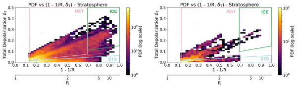
Figure 1 Point–density probability distribution of PSC measurements in the $(\mathrm{1}-\mathrm{1}/R),{\mathit{\delta }}_{\mathrm{T}}$ optical phase space. Left: full dataset including all Young-inverted cloud layers. Right: Young-optimized subset (Sect. 3.4). The full dataset cleanly separates STS, NAT and ice PSC clusters, while the Young-optimized subset suppresses most ice PSC occurrences. Regions identified as STS, NAT and ice PSCs are indicated by areas bounded by light-blue, pink and green contours, respectively.

5.1 Polar Stratospheric Clouds

Figure 1 shows the dataset point–density distribution in the $(\mathrm{1}-\mathrm{1}/R,{\mathit{\delta }}_{\mathrm{T}})$ phase space for the full dataset (left) and for the Young-optimized subset (right). The full dataset exhibits the expected tripartition of PSC microphysical types. Using the classification thresholds introduced in Sect. 4 – STS for $\mathrm{1.2}\le R\le \mathrm{3}$ and δ_TA<0.05, NAT for $\mathrm{1.2}\le R\le \mathrm{3}$ and δ_TA>0.10, and ice PSC for R≥3 and δ_TA>0.15 – the three regimes appear as well–separated clusters.

In the full dataset, the distribution shows points in the lower–left region $(\mathrm{1}-\mathrm{1}/R<\mathrm{0.8},{\mathit{\delta }}_{\mathrm{TA}}<\mathrm{0.05})$, corresponding to STS layers. This dense accumulation reflects the high frequency of STS conditions in the polar vortex and the fact that STS droplets produce only modest enhancements in backscatter and minimal depolarisation.

In the $(\mathrm{1}-\mathrm{1}/R,{\mathit{\delta }}_{\mathrm{T}})$ space, straight lines extending from the origin points towards a given value of δ_T=δ_TA for R=∞, and represent data from clouds with approximately constant microphysical morphology and increasing optical thickness (Adachi et al., 2001). The elongated diagonal cluster that occupies the intermediate depolarisation range (δ_TA≈0.05–0.15) and spans $\mathrm{1}-\mathrm{1}/R\approx \mathrm{0.2}$–0.6 can therefore be interpreted as coming from a sequence of NAT with similar particle habits but progressively larger optical depth, whose nonspherical particles increase both backscatter ratio and total depolarisation in a correlated manner, producing the observed tilted distribution.

A third, more diffuse lobe extends toward high values of both axes $(\mathrm{1}-\mathrm{1}/R>\mathrm{0.6},{\mathit{\delta }}_{\mathrm{T}}>\mathrm{0.15})$, marking ice PSC. The broad spread in this region reflects the wide variability of optical thickness, ice crystal habits and sizes, particularly under mesoscale cooling or in strongly supersaturated conditions. The patchier appearance of this region is a consequence of the relative rarity and intrinsic inhomogeneity of ice PSC, which often feature sharp vertical gradients and sublayering in externally mixed clouds.

In the Young-optimized subset, the distribution collapses into the lower portion of the diagram, with almost all ice PSC occurrences removed. The subset retains mainly STS and NAT layers, and even within the NAT regime the distribution becomes more compact. This reduction is a direct consequence of the Young homogeneity criteria: ice PSC commonly exhibit strong vertical gradients, multilayer structures, and abrupt transitions in both R and δ_T, which violate the symmetry, homogeneity, and smoothness conditions described in Sect. 3.4. The subset therefore isolates the most vertically uniform PSC – chiefly extensive STS and NAT layers embedded in homogeneous, aerosol–free background air.

We attribute this near-disappearance of ice PSC in the Young-optimized subset to the difficulty to identifying an ice PSC as an isolated layer, since these clouds tend to appear embedded within more complex PSC systems that include different cloud types. This is consistent with long-term lidar observations at other Antarctic sites. For example, the McMurdo PSC climatology of Adriani et al. (2004) documents that ice PSC exhibit a high degree of spatial and vertical variability, often appearing as thin, rapidly evolving layers embedded within or adjacent to other PSC types. These clouds frequently show sharp gradients in backscatter and depolarisation and are commonly associated with strong mesoscale temperature fluctuations. As a result, the atmospheric layers immediately above and below the cloud rarely satisfy the smooth, quasi-molecular conditions required by the Young optimization criteria.

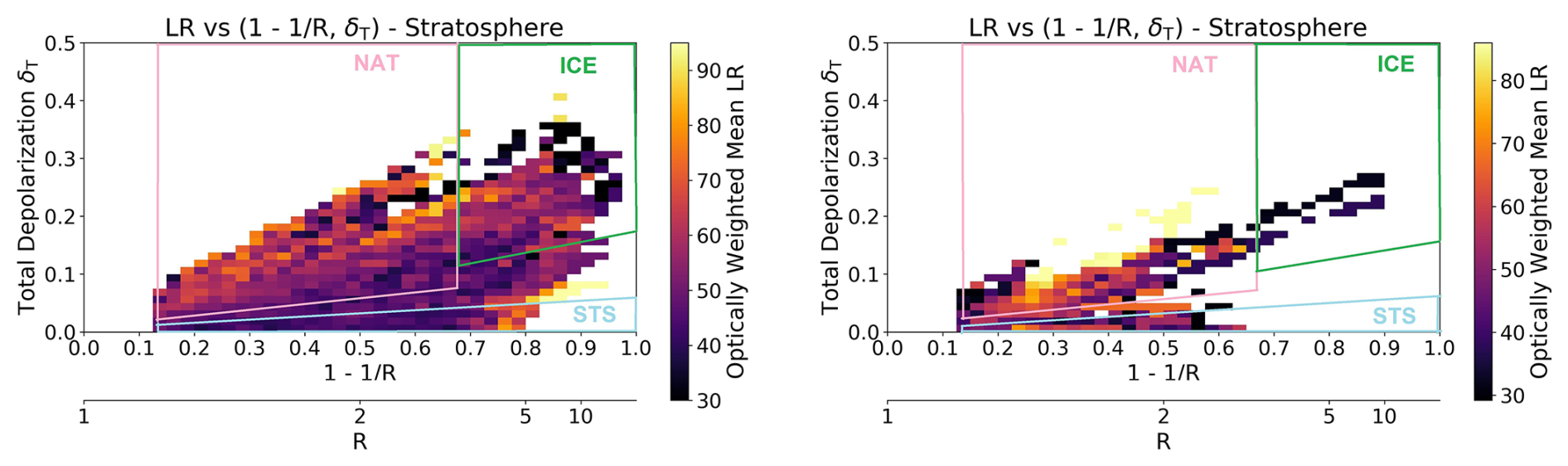
Figure 2 Optically weighted mean lidar ratio (LR) in the ($\mathrm{1}-\mathrm{1}/R,{\mathit{\delta }}_T$) phase space for PSC. Left: full dataset. Right: Young-optimized subset. Higher LR values are more frequently found in portions of the phase space associated with stronger backscatter enhancement and depolarization, although the relationship is not monotonic and shows substantial variability. In the Young-optimized subset most high-LR ice PSC disappear, likely because these layers do not satisfy the Young-optimization conditions.

In contrast, STS and NAT layers tend to be more vertically uniform and display more gradual transitions to the background aerosol, making them far more likely to fulfil the symmetry, smoothness and homogeneity constraints (Sect. 3.4). Thus, the Young-optimized subset naturally favours optically and dynamically simple layers, while filtering out the structurally complex and highly variable ice PSC identified in previous Antarctic climatologies (Santacesaria et al., 2001; Adriani et al., 2004).

To explore the dependence of the LR on backscatter and depolarization, we show in Fig. 2 the optically–weighted LR in the $(\mathrm{1}-\mathrm{1}/R,{\mathit{\delta }}_{\mathrm{T}})$ phase space. In this figure and similarly in Fig. 6 the term “weighted number of events” refers to a statistical representation in which each detected cloud layer contributes a single lidar ratio (LR), distributed over its vertical extent with optical weights proportional to the aerosol backscatter coefficient. The weights are normalized within each cloud so that all clouds contribute equally to the statistics, while optically dominant regions within each cloud exert a larger influence than optically thin boundaries. For the full dataset, LR tends to be larger in portions of the phase space associated with stronger depolarisation and larger backscatter ratios. However, this dependence is not monotonic and exhibits substantial scatter, reflecting both intrinsic microphysical variability and the occurrence of mixed or vertically structured PSC layers. Typical values range from ∼30–50 sr for STS to ∼40–70 sr for NAT and ice PSC.

Figure 3 One-dimensional probability density functions (PDFs) of the lidar ratio (LR) for the three PSC microphysical classes: STS, NAT, and ice. Left: full dataset. Right: Young-optimized subset. The full dataset shows broad and partially overlapping distributions, especially for ice PSC, due to their intrinsic microphysical variability and frequent embedding within mixed-phase structures. The Young-compatible subset yields narrower distributions for STS and NAT and retains only a few marginal ice PSC cases, illustrating the selective nature of the Young-compatible criteria. Dashed vertical lines indicate the optically weighted median LR for each class. The values reported in the legend give the median and the 25th–75th percentile range.

Figure 3 illustrates the LR probability distributions for the three PSC microphysical classes, comparing the full dataset (left) with the Young-optimized subset (right). In the full dataset, the three classes exhibit broad and partially overlapping distributions, reflecting both intrinsic microphysical variability and likely the frequent coexistence of multiple PSC types within the same vertical structure. STS show a relatively compact distribution centred around 38 sr (31–52 sr). NAT exhibits a wider spread, with a median of 49 sr (37–67 sr) and an extended high-LR tail. Ice PSC display the largest variability, ranging from ∼20 sr to very large values. This wide spread likely reflects not only the strong variability of crystal habits and growth conditions, but also the difficulty of isolating pure ice layers when they are embedded in mixed-phase structures; in such cases the retrieved LR represents an optical average over multiple particle populations, which tends to broaden the distribution and shift the median toward intermediate values.

In the Young-optimized subset, the LR distributions become markedly narrower for STS and NAT, while ice PSC nearly disappear because their edges typically show strong vertical inhomogeneities in both backscatter and depolarisation, causing them to fail the Young homogeneity and symmetry constraints. STS retain values around 38 sr (31–59 sr), but their distribution shows a weak apparent bimodality. A first accumulation appears near 35 sr, which is consistent with classical supercooled ternary solution droplets composed of aqueous sulfuric acid, nitric acid and water (Peter and Grooß, 2012; Carslaw et al., 1995).

A second, smaller accumulation occurs around 60 sr. This higher-LR feature may reflect layers in which STS droplets coexist with a minor fraction of nascent NAT particles, enhanced droplet growth under very cold conditions, or more generally mixed-phase PSC conditions, for which optical scattering can differ from that of pure single-component particle populations (Cairo et al., 2023). However, given the limited number of Young-optimized layers and the selectivity of the filtering criteria, this secondary accumulation should be interpreted cautiously.

NAT also shows an apparent multimodal structure, with one accumulation around 40 sr and another around 65–75 sr. Such a structure could be consistent with different NAT particle populations, for example smaller weakly depolarising particles and larger or more aspherical particles forming under colder conditions. However, the available sample does not allow us to demonstrate that these accumulations represent distinct and robust microphysical regimes. They may also be influenced by the Young selection criteria, residual vertical inhomogeneity, or limited sampling. We therefore interpret the multimodal behaviour as a suggestive feature of the Young-optimized subset, rather than as a definitive climatological result.

The ice PSC distribution in the Young subset is extremely compressed (32–38 sr), indicating that only marginal cases survive the selection, as their strong vertical gradients and likely external mixing with other PSC classes make them generally incompatible with the Young inversion constraints. Overall, the main robust result of the Young-optimized subset is therefore not the exact position of individual modes, but the narrowing of the LR distributions for the more homogeneous STS and NAT layers and the strong reduction of structurally complex ice PSC cases.

It is important to stress that the low median LR retrieved for ice PSC in the Young-optimized subset should not be interpreted as representative of typical ice PSC conditions. Rather, it reflects the strong selection against vertically inhomogeneous and multi-layer ice clouds inherent to the Young filtering, which preferentially retains only marginal, optically simple cases.

Overall, the comparison between the two datasets reveals that: (i) the full dataset captures the complete diversity of PSC optical behaviour, including mixed-phase and multi-layer structures; (ii) the Young-optimized subset isolates the most homogeneous and vertically uniform PSC layers, yielding tighter LR distributions and exposing microphysical substructures – such as the apparent bimodality in both STS and NAT – that are not easily discernible in the full dataset.

It is important to stress that the lidar-ratio values obtained from the Young-optimized subset should not be interpreted as a replacement for the full climatological distributions. Instead, the two datasets provide complementary information: the full dataset comprehends the effective lidar-ratio variability encountered in real atmospheric conditions, including mixed-phase and multilayer clouds, whereas the Young-optimized subset offers a lower-bound, physically conservative estimate applicable to idealised, vertically homogeneous layers.

Given the very limited number of cloud layers retained in the Young-optimized subset, no statistically meaningful analysis of their temporal distribution or of their association with specific dynamical or climatological conditions can be performed. The subset should therefore be interpreted strictly as a methodological benchmark, highlighting the behaviour of the Young inversion under near-ideal conditions, rather than as a representative sample of particular atmospheric states.

Figure 4 shows the vertical evolution of the median lidar ratio (LR) and its interquartile range for the three PSC classes. Only the full data set is discussed in terms of vertical variability, since the number of Young-optimized cases becomes too small at several altitudes to support a statistically representative profile.

Figure 4 Vertical profiles of the optically–weighted median lidar ratio (thick lines) and interquartile range (shaded bars) for PSC classes (STS, NAT, ice). Only the full dataset is displayed. STS show weak vertical dependence, NAT exhibit a progressive increase in LR toward colder upper–stratospheric levels, and ice PSC display the largest variability.

In the full data set, STS layers exhibit relatively low LR values (typically 35–45 sr) throughout the stratosphere, with a weak dependence on altitude up to about 22 km and a tendency toward slightly larger values at higher levels. This vertical stability reflects the microphysical nature of STS droplets, whose composition and size distribution evolve smoothly with temperature, yielding nearly constant optical properties over the probed altitude range.

NAT clouds display a broader LR distribution and a positive gradient with altitude, with median values increasing from ∼40 sr near 10–12 km to ∼55–60 sr above 20 km. This behaviour is consistent with the increase in NAT particle growth efficiency at lower temperatures in the upper stratosphere, favouring larger and more aspherical particles with enhanced extinction-to-backscatter ratios. The relatively coherent vertical progression also reflects the dominant occurrence of NAT over a wide altitude range.

Ice PSC show the largest variability and no simple monotonic trend. Median LR values span from about 45 sr to more than 70 sr, with substantial scatter at all altitudes. Such variability is expected, as ice PSC often form in dynamically complex environments influenced by rapid mesoscale temperature fluctuations, and multi-layer embedded structures. As frequently reported in PSC climatologies, ice layers may coexist with NAT or STS in vertically interleaved configurations, making the isolation of pure ice layers difficult. The broad LR distribution therefore reflects not only the intrinsic variability of ice crystal habits and growth histories, but also possible contamination from adjacent mixed-phase structures, which can bias LR toward intermediate values.

Figure 5 Normalized point–density PDF of tropospheric clouds in the $(\mathrm{1}-\mathrm{1}/R),{\mathit{\delta }}_{\mathrm{T}}$ phase space. Left: full dataset. Right: Young-optimized subset. Cirrus follow a continuous branch with increasing depolarization and backscatter enhancement, bounded by particle-depolarization isolines. The area bounded by green lines selects the well-developed ice clouds in the upper troposphere for further analysis. The reduced number of Young-optimized profiles mainly reflects the lower signal-to-noise ratio of the tropospheric channel rather than a microphysical selection.

5.2 Tropospheric Cirrus

The cirrus classification uses the same optical thresholds as ice PSC (R_def≥3 and δ_T>0.15), but restricted to altitudes below the climatological tropopause (12 km).

Figure 5 compares the point–density distribution in the $(\mathrm{1}-\mathrm{1}/R,{\mathit{\delta }}_{\mathrm{T}})$ phase space for tropospheric clouds, shown for the full dataset (left panel) and the Young-optimized subset (right panel).

The full dataset exhibits the expected continuous distribution of tropospheric cirrus in the ($\mathrm{1}-\mathrm{1}/R,{\mathit{\delta }}_T$) phase space. In this representation, the oblique directions are related to approximately constant particle depolarization: moving outward along such a direction mainly corresponds to increasing backscatter ratio R, while the intrinsic depolarizing character of the particles remains broadly similar. Thus, the main branch observed in Fig. 5 can be interpreted as a sequence of cirrus observations with comparable particle depolarization and progressively increasing optical contrast. The cirrus population does not separate into distinct clusters, but rather occupies a continuous domain extending toward larger values of both $\mathrm{1}-\mathrm{1}/R$ and δ_T.

In the Young-optimized subset (left panel), the number of available cases is significantly reduced. This reduction is expected and is primarily driven by the comparatively low signal-to-noise ratio of our tropospheric channels: the Young inversion requires well-defined cloud boundaries and smooth, extinction-corrected profiles both above and below the cloud, conditions that are often not met due to noisiness in our dataset. As a consequence, only the most structurally homogeneous, noise-free cirrus layers survive the Young criteria.

Despite the smaller sample, the locus of points retained by the Young selection remains consistent with the morphology of the full dataset: the same positive correlation between δ_T and $\mathrm{1}-\mathrm{1}/R$ is observed, and the high-density region corresponds to the same domain characteristic of mid-latitude cirrus. Overall, the comparison shows that: (i) the Young method does not introduce a systematic bias in the microphysical phase space of tropospheric clouds, and (ii) the reduced population mainly reflects $S/N$ limitations rather than a physical filtering of specific cirrus types.

Figure 6 shows the distribution of tropospheric measurements coloured by the optically weighted mean lidar ratio (LR). The left panel corresponds to the full dataset, while the right panel shows only those cloud layers that satisfy all Young inversion constraints. Across this full range, LR values span approximately 20–80 sr, consistent with climatological cirrus studies (e.g. Chen et al., 2002; Yorks et al., 2011; Giannakaki et al., 2007). A weak increase of LR toward higher depolarisation is also visible, perhaps reflecting the tendency of larger and more complex ice crystals to exhibit higher extinction-to-backscatter ratios. The clustering of data at $(\mathrm{1}-\mathrm{1}/R)\simeq \mathrm{0.8}$–0.9, i.e. R≃5–10, corresponds to the optically thickest cirrus layers in our sample and is associated with LR values ≃50.

Figure 6 Optically–weighted mean lidar ratio (LR) for tropospheric clouds in the $(\mathrm{1}-\mathrm{1}/R),{\mathit{\delta }}_{\mathrm{T}}$ optical phase space. Left: full dataset. Right: Young-optimized subset. The full dataset spans LR ∼20–80 sr with a modal region near 35–55 sr. The Young subset collapses into a narrower region (LR ∼30–40 sr), reflecting the removal of clouds with noisy boundaries or strong vertical gradients while preserving the central microphysical structure of the full population.

The Young-optimised subset (left panel) occupies a narrower region of the same phase space, forming a well-defined ridge of points aligned toward δ_TA≃0.30 and a few other scattered points, with low to intermediate values of $\mathrm{1}-\mathrm{1}/R$. This contraction is expected, since the Young inversion filters out layers with insufficient signal-to-noise ratio – conditions at the boundaries of the cloud, that are common in the tropospheric channel. Despite the reduced sampling, the LR distribution in the Young subset remains fully consistent with that of the full dataset. The retrieved values cluster tightly around 31–42 sr, not far from the modal LR range seen in the unfiltered population. High-LR outliers (>60 sr) visible in the full dataset are absent. Overall, the comparison demonstrates that the Young-optimized subset is preserving the central microphysical signal of the full dataset. The modal LR is unchanged, and the phase-space structure (in particular the organisation along oblique lines of constant particle depolarisation) is maintained.

Figure 7 shows the probability density function (PDF) of the lidar ratio (LR) for tropospheric cirrus, respectively for the Young-optimized subset (right) and for the full tropospheric data set (left).

Figure 7 One-dimensional probability density functions (PDFs) of the lidar ratio (LR) for tropospheric cirrus. Left: full dataset. Right: Young-optimized subset. The full dataset shows the broader LR variability of the observed cirrus population, whereas the Young-compatible subset retains only a very small number of layers satisfying the stricter homogeneity criteria. Dashed vertical lines indicate the optically weighted median LR of each distribution. The values reported in the legend give the median and the 25th–75th percentile range.The Young-compatible cirrus distribution should therefore be interpreted only as a methodological benchmark and not as a representative cirrus climatology.

In the Young-optimized subset, the LR distribution is extremely compact, with a median value of ∼ 40 sr and an interquartile range confined to ∼ 32–40 sr The narrowness of the distribution reflects the paucity of the dataset induced by the stringent homogeneity requirements of the Young inversion and is likely not representative of the whole variability of the LR. The full data set displays a much broader LR distribution, with a median of ∼ 50 sr and an extended upper tail reaching 80 sr. This broader range is consistent with previous Raman-lidar climatologies, which report LR values of 20–40 sr for thin cirrus and 40–70 sr (or higher) for vertically extended or multi-layer structures. The larger LR values in the full population may likely correspond to clouds with strong internal variability or large, complex ice habits such as bullet rosettes or aggregates, which increase the extinction-tobackscatter ratio, although biases induced by the Young inversion procedure cannot be excluded. The vertical profile of cirrus LR shown in Fig. 8 is relatively stable with altitude when the interquartile variability is taken into account. Median values remain within the range reported by previous visible-wavelength cirrus lidar studies, and no strong monotonic dependence on height is evident. This is consistent with the results of Giannakaki et al. (2007), who found no clear dependence of cirrus LR on cloud temperature and thickness, and with Voudouri et al. (2020), who reported that cirrus LR is generally quite constant with temperature, although with substantial variability. A weak decrease of LR at the highest altitudes may be present, which would not be inconsistent with Chen et al. (2002), who reported lower LR values for cirrus above about 15 km. However, in the present dataset this feature should be interpreted cautiously because of the limited sampling in some altitude bins and the broad variability of cirrus optical properties.

Figure 8 Vertical profile of optically weighted median lidar ratio (LR) for tropospheric cirrus. Only the full dataset is displayed. The median LR profile is relatively stable with altitude within the observed variability; any weak decrease at the highest altitudes should be interpreted cautiously.

6 Discussion

The Young inversion relies on the assumption that the particle backscatter ratio is identical immediately above and below a homogeneous cloud layer. This condition is often met for vertically homogeneous layers (e.g. extended STS or NAT PSC, or thick homogeneous cirrus), but it can be severely violated in the presence of sharp vertical gradients and multiple sublayers, such as for ice PSC or dynamically perturbed cirrus. The comparison between the full data set and the Young-optimized subset therefore is aimed at providing a direct, observation-based quantification of how real polar clouds depart from these ideal assumptions, and how such departures bias the retrieved lidar ratio. Unfortunately, for tropospheric ice clouds, the Young-optimized dataset is probably too sparse to be statistically significant.

Temperature provides an additional physical coordinate for interpreting these results. Altitude alone should not be interpreted as the controlling variable for LR; rather, altitude acts as a proxy for the thermodynamic regime sampled by the cloud. For PSCs, the relevant temperature thresholds are those controlling STS growth, NAT formation and ice nucleation. Ice PSC are expected near or below the frost-point temperature, whereas NAT and STS can occur at warmer temperatures within the PSC stability range. This is important for the interpretation of the LR distributions: layers sampled close to the NAT/ice transition may contain externally mixed or vertically interleaved particle populations, so that the retrieved layer-mean LR represents an effective value rather than a pure ice or pure NAT optical signature. Similarly, the increase of NAT LR with altitude is interpreted here primarily as a temperature-related effect, reflecting colder conditions that favour larger or more aspherical NAT particles, rather than as a direct dependence of LR on geometric height.

For the cloud particles considered in this study, an increase in the lidar ratio generally reflects a shift toward larger or more aspherical particles. Since the extinction coefficient scales approximately with particle cross-section while the relative backscatter efficiency decreases for larger or more complex particles, the ratio $\mathit{\alpha }/\mathit{\beta }$ increases as particle size grows. This behaviour is well established in modelling studies for STS (Luo et al., 2003), NAT (Höpfner et al., 2006), and ice PSC (Reichardt et al., 2004), where higher LR values correspond to particles with larger effective radii, broader size distributions, or more aspherical shapes. This interpretation is intended for PSC and cirrus cloud particles and should not be generalized to all atmospheric aerosol types, for which absorption, composition and internal mixing may alter the relationship between particle properties and LR. Therefore, the observed increase of LR with altitude for NAT, and the large LR variability of ice PSC, are consistent with the presence of progressively larger or more complex particles under colder stratospheric conditions.

The PSC populations are cleanly separated in the $(\mathrm{1}-\mathrm{1}/R,{\mathit{\delta }}_{\mathrm{T}})$ phase space, with STS at low depolarisation, NAT at intermediate values, and ice PSC at high depolarisation and larger variability. The optically weighted lidar ratios obtained from the full data set cluster around

$$\begin{array}{}\text{(8)}& {\mathrm{LR}}_{\mathrm{STS}}\approx \mathrm{38}\mathrm{sr},{\mathrm{LR}}_{\mathrm{NAT}}\approx \mathrm{49}\mathrm{sr},{\mathrm{LR}}_{\mathrm{ice}}\approx \mathrm{52}\mathrm{sr},\end{array}$$

with ice PSC spanning a broad range extending up to ∼70 sr. These values fall squarely within the microphysically expected regimes: Mie calculations predict STS droplets to exhibit LR in the 30–40 sr range with weak sensitivity to size and composition (Luo et al., 2003; Peter and Grooß, 2012), while irregular NAT particles generally yield LR between 40 and 60 sr (Reichardt et al., 2004; Höpfner et al., 2006). Ice PSC show the largest variability due to the strong dependence of crystal habit and size on cooling history, sedimentation and mesoscale temperature variability (Reichardt et al., 2004; Tritscher et al., 2021).

The Young-optimized subset selectively removes layers where the Young inversion is more likely to fail. Its effect differs among PSC classes. For STS and NAT, the filtering mainly narrows the LR distributions and shifts the median values to:

$$\begin{array}{}\text{(9)}& {\text{LR}}_{\mathrm{STS}}\approx \mathrm{41}\mathrm{sr};{\text{LR}}_{\mathrm{NAT}}\approx \mathrm{59}\mathrm{sr}\end{array}$$

For ice PSC, however, the number of retained layers becomes too small to define a representative lidar-ratio statistic. The apparent decrease of the ice-PSC median LR in the Young-optimized subset should therefore not be interpreted as a robust microphysical result. It more likely reflects the preferential exclusion of vertically structured and mixed-phase ice PSC layers, leaving only a few optically simple or marginal cases. This limitation is particularly important because only 2 ice PSC layers are retained in the Young-optimized subset, compared with 9 in the full dataset, so that the apparent median value is highly uncertain and should not be treated as statistically representative.

The apparent multimodal structure observed in the Young-optimized STS and NAT distributions should also be interpreted cautiously. These modes may reflect real microphysical variability, such as different particle sizes, degrees of asphericity, or mixed STS/NAT conditions. However, they may also be affected by the limited number of retained layers and by the selectivity of the Young-optimized criteria. We therefore do not interpret the modes as conclusive evidence for distinct microphysical regimes, but rather as suggestive features that would require larger samples or independent microphysical constraints to be confirmed.

Although the Young-optimized criteria are applied to regions outside the cloud, they are sensitive to any departure from the ideal conditions required by the Young inversion. If the cloud is a single, vertically homogeneous layer embedded in a uniform background, the extinction correction based on a trial LR modifies the attenuated signal in a smooth and self-consistent manner, yielding nearly identical values of the corrected backscatter ratio above and below the cloud. In contrast, if the cloud contains internal sublayers with different extinction-to-backscatter ratios, no single LR can adequately describe the entire layer. The inversion may then overcorrect one part of the cloud and undercorrect another, with these errors propagating into the extinction-corrected signal outside the cloud (Ansmann et al., 1990). As a result, the corrected backscatter ratio may become asymmetric above and below the cloud and may exhibit enhanced variance or gradients in the external control windows.

However, a failure of the Young-optimized criteria cannot be attributed uniquely to internal cloud inhomogeneity. Similar signatures may also be produced by residual aerosol or thin undetected layers in the external reference windows, vertical gradients in the background atmosphere, uncertainties in cloud-boundary detection, or reduced signal-to-noise ratio. For this reason, the Young-optimized fraction reported in Table 1 should be interpreted operationally: it quantifies the fraction of cloud layers for which the combined cloud-background system satisfies the symmetry, smoothness and homogeneity conditions required for a robust Young inversion. It should not be interpreted as a direct or universal estimate of the fraction of internally homogeneous clouds. This interpretation is consistent with previous PSC studies showing that polar stratospheric clouds often display substantial structural and compositional variability. Ground-based and spaceborne lidar observations have shown that PSC fields may contain externally mixed or vertically layered STS, NAT and ice particle populations, and that ice PSC in particular are often associated with sharp gradients, mesoscale temperature perturbations and complex vertical structure (Pitts et al., 2018; Snels et al., 2021; Di Liberto et al., 2024). To our knowledge, however, directly comparable Young-optimized fractions based on the same top-bottom consistency and external-window homogeneity criteria have not been reported previously. The fractions reported here should therefore be regarded as dataset- and method-specific indicators of compatibility with the Young inversion assumptions. The apparently larger Young-optimized fraction for ice PSC should not be overinterpreted, because it is based on only nine ice PSC layers in the full dataset. The more robust information is the very small absolute number of retained ice PSC cases, which confirms that the Young-optimized ice PSC subset is not statistically representative.

The LR values retrieved in this work are consistent with previous lidar studies. Early ground-based Raman and depolarisation lidar measurements reported 30–40 sr for STS and 40–60 sr for NAT or mixed-phase PSC (Reichardt et al., 2004, 2002), with ice PSC occasionally exceeding 60 sr during intense mountain-wave events. CALIOP climatologies similarly employ type-dependent LR values of 30 sr (STS), 50 sr (NAT) and 25–60 sr (ice), depending on layer structure (Pitts et al., 2009, 2018). At Concordia, previous PSC studies primarily characterised the backscatter–depolarisation phase space (Snels et al., 2021; Di Liberto et al., 2024), and the present analysis extends this framework by adding quantitative LR retrievals, confirming the internal consistency between microphysical typing and optical properties.

Tropospheric cirrus above Dome C exhibit a median LR value of LR_cirrus ≈ 50 sr in the full dataset, with a tail extending to lower values. These values are consistent with Raman lidar studies reporting typical visible-wavelength LR of 20–40 sr for thin cirrus and 40–50 sr for vertically extended or multi-layer clouds (Ansmann et al., 1992; Immler and Schrems, 2002; Haarig et al., 2016; Wang et al., 2020).

Under Young-optimized conditions, the median LR decreases to LR_cirrus≈40 sr and the distribution narrows. The lower-bound value of ∼30 sr is physically consistent with homogeneous, optically simple cirrus and agrees with Raman-lidar observations at other high-latitude sites, although the scarcity of data for the Young-optimized dataset suggest to pose some caution on the representativeness of such results.

An interesting outcome is the difference between the LR of ice PSC and cirrus, despite both being composed of crystalline ice. Ice PSC observed above Dome C typically span 40–60 sr with excursions beyond 70 sr, while cirrus peak around 45–50 sr and rarely approach PSC-like values.

This contrast is consistent with their different microphysical pathways and with the effective optical complexity sampled by lidar observations. Ice PSC form at extremely low temperatures (T<188 K) through heterogeneous nucleation on pre-existing STS or NAT particles. As a consequence, ice PSC crystals are generally smaller than cirrus crystals but are expected to be highly aspherical and poorly constrained in habit. Their optical response is further complicated by frequent coexistence with NAT or STS layers and by strong vertical inhomogeneities, which can enhance the effective lidar ratio retrieved for the layer.

Conversely, cirrus clouds form either in situ or by convective detrainment in a warmer and moister environment, allowing the growth of larger ice crystals with well-developed habits (columns, plates, bullet rosettes, aggregates). Despite their larger size, cirrus layers are often optically more homogeneous, leading to more stable LR values and fewer extreme excursions.

Thus, the observed differences between PSC and cirrus LR can be physically explained by the combined effects of particle habit, mixing state, and vertical homogeneity, rather than by crystal size alone.

The present analysis does not include a direct satellite-based validation of the retrieved LR values. Such a comparison would require strict temporal and spatial collocation, consistent cloud-boundary definitions, and a careful treatment of the different retrieval assumptions used by ground-based elastic lidar and spaceborne lidar products. In the case of ATLID/EarthCARE, an additional complication is the wavelength difference between the 532 nm measurements analysed here and the 355 nm ATLID observations. However, the statistical consistency between the Dome C ground-based lidar record and CALIOP PSC observations has already been assessed. Snels et al. (2021) compared the statistical occurrence and composition of PSCs observed at Dome C with CALIOP observations over the same Antarctic sector, showing that the ground-based record is broadly consistent with the spaceborne PSC climatology in terms of occurrence and microphysical classification. A similar comparison was carried out for the PSC observed at McMurdo Station (77°50^′ S, 166°40^′ E; 183 m a.s.l.; Snels et al., 2019). The LR climatology presented here therefore builds on an observational framework whose statistical representativeness has already been documented, while extending it by providing layer-mean LR estimates from the ground-based Young inversion. These values may serve as a ground-based statistical reference for future dedicated collocation studies with CALIOP legacy products and EarthCARE/ATLID observations.

7 Conclusions

We presented a 3-year dataset (2022–2024) of ground-based polar stratospheric cloud (PSC) and cirrus observations performed at Dome C using an elastic backscatter lidar with depolarization capability. For the first time at this site, lidar ratios (LR) were retrieved systematically using the Young inversion method. The resulting dataset provides a physically consistent characterisation of PSC and cirrus optical properties and establishes a reference framework for future studies in Antarctica.

The retrieved LR distributions for the full PSC population peak around ∼38 sr for STS, ∼49 sr for NAT, and ∼52 sr for ice PSC, with percentiles spanning the ranges (31–52), (37–67), and (41–66) sr, respectively. These values are consistent with expectations from optical modelling and with previous Raman and depolarisation lidar studies. Importantly, the broad LR distribution of ice PSC is likely not only a signature of intrinsic microphysical variability, but also a consequence of their frequent coexistence with STS and NAT within mixed-phase structures. Under such conditions, retrieving a single, layer-integrated LR inevitably leads to values that represent an aggregate of multiple particle types rather than a pure ice signature.

Tropospheric cirrus exhibit a median lidar ratio of ∼ 50 sr (33–52 sr), while the Young-optimized subset converges toward lower values around ∼ 40 sr.

Joint analysis in the $(\mathrm{1}-\mathrm{1}/R,{\mathit{\delta }}_{\mathrm{T}})$ space confirms the clear separation of PSC regimes and the tight clustering of cirrus. The observed distributions agree with theoretical phase-space structures: lines of constant particle depolarisation correspond to families of optically thickening clouds, while the elongation of the NAT cluster reflects increasing optical depth at nearly constant morphology.

Overall, this work provides a long-term, internally consistent statistic of PSC and cirrus lidar ratios at Dome C and a quantitative assessment of how real clouds retrievals deviate from the assumptions underlying the Young method. An important implication of this analysis is that lidar-ratio statistic cannot be uniquely defined without reference to the validity of the underlying inversion assumptions. By explicitly distinguishing between full and Young-optimized datasets, this work provides both a realistic representation of the variability encountered in operational conditions and a conservative benchmark applicable to idealized homogeneous cloud layers.

The dataset and methods developed here may support ongoing efforts to evaluate PSC microphysical transitions, diagnose stratospheric temperature anomalies, and improve spaceborne lidar retrievals in polar regions.

A key outcome of this work is therefore not a single set of lidar-ratio values, but a quantitative framework that links lidar-ratio statistics to the validity of the underlying inversion assumptions. This framework enables a transparent and physically consistent use of ground-based lidar observations in both climatological and methodological contexts.

The LR statistics presented here also provide a useful ground-based statistical reference for the interpretation of spaceborne lidar observations. This is particularly relevant in view of the CALIOP legacy PSC record and of the current EarthCARE/ATLID mission. Previous statistical comparisons at Dome C have shown that the ground-based lidar record captures PSC occurrence and composition features broadly consistent with CALIOP-based Antarctic climatologies. The present study extends this framework by adding observational constraints on layer-mean LR.