Radar data smoothing using the Discrete Cosine Transform: a fast spectral domain algorithm

This study introduces a computationally efficient and methodologically robust approach for smoothing radar data using the Discrete Cosine Transform (DCT). Traditional spatial convolution methods for noise reduction in polar coordinates suffer from geometric inconsistencies and prohibitive computational costs, particularly when implementing range-dependent dynamic kernels to maintain physical scale. We propose a spectral-domain alternative that utilizes the convolution theorem to perform equivalent smoothing operations. By deriving analytical transfer functions for various kernels – including Boxcar, Gaussian, and Savitzky–Golay – we demonstrate that the DCT method achieves identical performance to spatial convolution while effectively handling boundary conditions. Performance benchmarks on real C-band weather radar data reveal that the DCT-based approach offers speedup factors exceeding 800 times for large kernel sizes. Furthermore, for large-scale datasets (180 million pixels), equivalent processing time is reduced from over 1 h to under 18 s. The proposed method ensures physically consistent smoothing across ranges, preserving small-scale meteorological features while enabling real-time data quality improvement.

1 Introduction

Weather radar observations often show large spatial variability, which is typically exacerbated by various sources of noise and observational artifacts. Some gradients are related to the nature of precipitation, others result from oversampling, and non-meteorological features such as partial or complete beam blockage (Hubbert et al., 2009; Atlas, 1990), data gaps related to data filtering, non-uniform beam filling around cloud edges (Bringi and Chandrasekar, 2001), and range-dependent beam broadening (e.g. Torres and Zrnić, 2003; Ivić et al., 2003). While significant progress has been made in removing structured non-meteorological echoes (e.g., ground clutter filtering), high-frequency fluctuations in the signal remains a computational expensive process, particularly for improving data quality for visualization and automated analysis.

Traditional spatial domain smoothing techniques, such as the moving window average (boxcar filter; Smith, 1997), have been widely used to mitigate this “noise”. However, applying these filters in the native polar coordinate system of radar data presents geometric challenges. A constant window size in the range-angle domain corresponds to a physically varying spatial scale; a small window at close range covers a much smaller physical area than the same window at long range. This leads to inconsistent smoothing: data at long ranges may be undersmoothed while data at close ranges may be oversmoothed, or vice-versa. To visualize this issue, Fig. 1 illustrates how a constant angular window corresponds to drastically different physical areas at different ranges, highlighting the need for range-dependent kernel adaptation which is computationally expensive in the spatial domain.

Figure 1 Conceptual comparison of coordinate distortion for (a) a window of constant size in grid space (range-angle indices) that corresponds to (b) physically different areas in a physical space depending on the range. At close range, the physical area is small, whereas at far range, it expands significantly. This distortion necessitates dynamic kernel sizing to maintain a constant physical smoothing scale.

In this work, we propose a spectral-domain approach using the Discrete Cosine Transform (DCT; Ahmed et al., 1974) to perform radar data smoothing in the native polar coordinate space. This smoothing technique help us to filter out high-frequency oscillations in the signal that is treated as “noise”. We demonstrate that DCT-based convolution offers a computationally efficient and mathematically equivalent alternative to spatial convolution, with the added benefit of easily handling range-dependent kernel scaling and boundary conditions that mitigate artifacts like the Gibbs phenomenon. Specifically, the DCT method allows us to perform convolution in O(Nlog N) time, which is significantly faster than the O(N⋅W²) complexity of spatial convolution with large windows. This speed advantage allows for real-time processing of large radar volumes with physically correct range-variant smoothing, which was previously computationally prohibitive. DCT method requires a complete, continuous dataset. Unlike spatial convolution which can simply skip invalid pixels (NaNs) or adjust normalization, spectral transforms technically require defined values everywhere. Therefore, data gaps due to filtering or beam blockage must be filled (e.g., via interpolation) prior to applying the transform. This prefilling requirement is a known limitation of spectral methods; its consequences and the alternative strategies that address them are discussed in Sect. 3.

This paper is organized as follows. Section 2 establishes the theoretical framework, detailing the convolution theorem and its application in polar coordinates. Section 3 demonstrates the application of this method to real radar observations. Section 4 presents a performance benchmark comparing the proposed DCT method against traditional spatial algorithms. Finally, Sect. 5 discusses the implications and Sect. 6 concludes the study.

2 Theoretical Framework and Geometric Considerations

2.1 Convolution Theorem and Transfer Function

The fundamental mathematical principle underlying this work is the Convolution Theorem, which states that convolution in the spatial domain is equivalent to point-wise multiplication in the spectral domain (Oppenheim et al., 1999). For two discrete signals f[n] and g[n], their linear convolution (f×g)[n] corresponds to:

$$\begin{array}{}\text{(1)}& \mathcal{T}\mathit{\{}\mathit{f}\times \mathit{g}\mathit{\}}=\mathcal{T}\mathit{\left\{}f\mathit{\right\}}\cdot \mathcal{T}\mathit{\left\{}g\mathit{\right\}}\end{array}$$

where 𝒯 denotes a linear transform. While this is commonly associated with the Discrete Fourier Transform (DFT) under periodic boundary conditions (circular convolution), it also applies to the Discrete Cosine Transform (DCT) under the assumption of symmetric boundary conditions (Makhoul, 1980). We utilize the DCT-II, defined for a signal x[n] of length N as:

$$\begin{array}{}\text{(2)}& X\left[k\right]=\mathrm{2}\sum _{n=\mathrm{0}}^{N-\mathrm{1}}x\left[n\right]\cos \left({\displaystyle \frac{\mathit{\pi }k(\mathrm{2}n+\mathrm{1})}{\mathrm{2}N}}\right),\mathrm{0}\le k<N\end{array}$$

The DCT-II corresponds to a discretization of the Neumann boundary condition (zero derivative at the endpoints) in the continuum limit. In the discrete domain, this implies a half-sample symmetric extension of the data at the boundaries (Strang, 1999).

Ng et al. (1999) demonstrated that while the DFT diagonalizes circulant matrices (periodic convolution), the DCT-II diagonalizes (or approximately diagonalizes, depending on the kernel symmetry) matrices with Toeplitz-plus-Hankel structure. This structure mathematically represents the sum of a standard linear convolution (Toeplitz) and the convolution with the reflected data at the boundaries (Hankel). Therefore, point-wise multiplication in the DCT domain is equivalent to spatial convolution where data outside the domain is modeled as a symmetric reflection of the data inside, effectively mitigating the edge artifacts associated with periodic DFT assumptions.

For a symmetric filter h[n] of width M (where M is odd), centered at n=0, the coefficients are $\mathit{h}\left[n\right]=\mathrm{1}/M$ for $\left|n\right|\le (M-\mathrm{1})/\mathrm{2}$ and 0 otherwise. The frequency response (or transfer function) H[k] in the DCT domain corresponds to the DFT of the symmetric extension of the filter. Since h[n] is real and even, its frequency response is given by the sum of cosine terms:

$$\begin{array}{}\text{(3)}& \mathbf{H}\left[k\right]=\sum _{n=-(M-\mathrm{1})/\mathrm{2}}^{(M-\mathrm{1})/\mathrm{2}}h\left[n\right]\cos \left({\displaystyle \frac{\mathit{\pi }kn}{N}}\right)\end{array}$$

Substituting $h\left[n\right]=\mathrm{1}/M$:

$$\begin{array}{}\text{(4)}& \begin{array}{rl}{\displaystyle }\mathbf{H}\left[k\right]& {\displaystyle }={\displaystyle \frac{\mathrm{1}}{M}}\left(\cos \right(\mathrm{0})+{\sum }_{n=\mathrm{1}}^{(M-\mathrm{1})/\mathrm{2}}\cos \left({\displaystyle \frac{\mathit{\pi }kn}{N}}\right)\\ {\displaystyle }& {\displaystyle }+{\sum }_{n=-(M-\mathrm{1})/\mathrm{2}}^{-\mathrm{1}}\cos \left({\displaystyle \frac{\mathit{\pi }kn}{N}}\right))\end{array}\end{array}$$

Since $\cos (-x)=\cos \left(x\right)$, the negative indices sum is identical to the positive indices sum. Therefore, for a boxcar filter of width M in the DCT-II domain, the transfer function H[k] is given by:

$$\begin{array}{}\text{(5)}& \mathbf{H}\left[k\right]={\displaystyle \frac{\mathrm{1}}{M}}\left(\mathrm{1}+\mathrm{2}\sum _{j=\mathrm{1}}^{(M-\mathrm{1})/\mathrm{2}}\cos \left({\displaystyle \frac{j\mathit{\pi }k}{N}}\right)\right)\end{array}$$

To generalize this for continuous widths W (essential for polar coordinate smoothing where the effective kernel width varies continuously with range), we utilize the Dirichlet kernel identity (Levi, 1974). This extension effectively defines a continuous spectral filter that approximates a fractional-width moving average:

$$\begin{array}{}\text{(6)}& \mathrm{1}+\mathrm{2}\sum _{j=\mathrm{1}}^K\cos \left(j\mathit{\theta }\right)={\displaystyle \frac{\sin \left(\right(K+\mathrm{1}/\mathrm{2}\left)\mathit{\theta }\right)}{\sin (\mathit{\theta }/\mathrm{2})}}\end{array}$$

This is a standard result in Fourier analysis (Oppenheim et al., 1999). Substituting $K=(W-\mathrm{1})/\mathrm{2}$ and $\mathit{\theta }={\mathit{\omega }}_k=\left(\mathit{\pi }k\right)/N$, we obtain the analytical transfer function:

$$\begin{array}{}\text{(7)}& \mathbf{H}\left[k\right]={\displaystyle \frac{\mathrm{1}}{W}}{\displaystyle \frac{\sin (W{\mathit{\omega }}_k/\mathrm{2})}{\sin ({\mathit{\omega }}_k/\mathrm{2})}}\end{array}$$

Note that ${lim}_{{\mathit{\omega }}_k\to \mathrm{0}}\mathbf{H}\left[k\right]=\mathrm{1}$. This closed-form expression allows us to compute the smoothing operation efficiently for any real-valued width W, mitigating discretization errors associated with forcing integer kernel sizes. It is important to emphasize that while we refer to this as an “analytical boxcar convolution” due to its spatial equivalent, in the DCT domain it is strictly a spectral filter. This distinction allows us to bypass the constraints of discrete grid indices entirely, operating on the continuous frequency response of the underlying function rather than a pixelated approximation.

2.2 2D Convolution and Separability

The 2D spatial convolution of a matrix x[m,n] with a kernel h[m,n] is defined as:

$$\begin{array}{}\text{(8)}& \mathbf{y}[m,n]=(\mathbf{x}\times \mathbf{h})[m,n]=\sum _i\sum _{j}x[m-i,n-j]h[i,j]\end{array}$$

In our experiments, we use a boxcar filter of size M×M. A key property of this filter is its separability, meaning it can be decomposed into two 1D filters:

$$\begin{array}{}\text{(9)}& \mathbf{h}[m,n]=h_{\text{ang}}\left[m\right]\cdot h_{\text{range}}\left[n\right]\end{array}$$

where h_ang and h_range are 1D boxcar filters. Similarly, the 2D DCT is separable:

$$\begin{array}{}\text{(10)}& {\mathbf{X}}_{\text{2D}}[u,v]={\text{DCT}}_{\text{range}}\left({\text{DCT}}_{\text{ang}}\right(\mathbf{x}[m,n]\left)\right)\end{array}$$

For a standard separable convolution with a constant kernel, the 2D transfer function is simply the outer product of the 1D transfer functions: ${\mathbf{H}}_{\text{2D}}[u,v]=H_{\text{ang}}\left[u\right]\cdot H_{\text{range}}\left[v\right]$.

2.3 2D Convolution in Polar Coordinates

Radar observations are collected on a polar grid (r,θ) through scanning strategies such as the Plane Position Indicator (PPI) for horizontal surveys or the Range Height Indicator (RHI) for vertical cross-sections. While these datasets are frequently projected onto Cartesian coordinates for integration with numerical models, performing smoothing directly in the native polar domain avoids interpolation artifacts but introduces geometric complexities. To ensure physically consistent smoothing, the effective kernel size must dynamically adapt to the range-dependent expansion of the radar sampling volume, accounting for the linear increase in transverse resolution with distance from the sensor. Throughout this section, “angle” refers to the polar angular coordinate θ, which is the azimuth for PPI scans and the elevation for RHI scans; the analysis applies to either case.

We adopt three related kernel-width quantities to describe this range dependence. Let W_phys denote the physical smoothing width in units of length (e.g., meters or kilometers), which is held constant in the angle direction at every range. The equivalent width in pixels is $W=W_{\text{phys}}/\left(r\mathrm{\Delta }\mathit{\theta }\right)$, a continuous real-valued parameter identical to the W of Eq. (7). In the range dimension the resolution is constant, so a fixed kernel is used. In the angle dimension the arc length Δs=rΔθ grows with range, so the discrete kernel applied at each angle index is N_ang(r), the odd integer obtained by symmetrically rounding W to keep the kernel centered on the target cell:

$$\begin{array}{}\text{(11)}& N_{\text{ang}}\left(r\right)=\mathrm{2}⌊{\displaystyle \frac{W_{\text{phys}}}{\mathrm{2}r\mathrm{\Delta }\mathit{\theta }}}⌋+\mathrm{1}\end{array}$$

The factor $\mathrm{1}/r$ makes W decrease with range even though W_phys is constant, so N_ang(r) is small near the radar and grows toward long range.

In the spectral domain this range dependence implies that the operation cannot be expressed as a single global 2D transfer function. Instead we treat it as a sequence of separable operations: for each angle α, angle-direction smoothing uses a range-specific 1D filter h_ang[α], which in the 1D DCT along the angle direction corresponds to multiplying by a range-dependent transfer-function matrix H_ang[α,v]. Range smoothing uses a fixed filter, which in the 1D DCT along the range direction corresponds to multiplying by a constant transfer function H_range[u].

The separable form is exact for a kernel that is itself separable: a 2D boxcar $h[m,n]=h_{\text{ang}}\left[m\right]\cdot h_{\text{range}}\left[n\right]$ is mathematically identical to two sequential 1D boxcars, not an approximation of one. In polar geometry the resulting effective kernel is intentionally axis-aligned in (range, angle) to match the polar sampling volume (Bringi and Chandrasekar, 2001), so the anisotropy of the smoothing is the anisotropy of the radar geometry, not an artifact of the method.

The full 2D smoothing operation Y can be decomposed into a sequence of separable steps. First, we perform the angle-direction smoothing, whose transfer function depends on range:

$$\begin{array}{}\text{(12)}& {\displaystyle }{\stackrel{\mathrm{̃}}{\mathbf{X}}}_{\text{ang}}& {\displaystyle }={\text{DCT}}_{\text{ang}}\left(X\right)\text{(13)}& {\displaystyle }{\stackrel{\mathrm{̃}}{\mathbf{Y}}}_{\text{ang}}& {\displaystyle }={\stackrel{\mathrm{̃}}{\mathbf{X}}}_{\text{ang}}\circ {\mathbf{H}}_{\text{ang}}\text{(14)}& {\displaystyle }{\mathbf{Y}}_{\text{ang}}& {\displaystyle }={\text{IDCT}}_{\text{ang}}\left({\stackrel{\mathrm{̃}}{\mathbf{Y}}}_{\text{ang}}\right)\end{array}$$

where ∘ denotes the Hadamard (element-wise) product and H_ang is the matrix of range-dependent transfer functions. Next, we apply the constant smoothing along the range direction:

$$\begin{array}{}\text{(15)}& {\displaystyle }{\stackrel{\mathrm{̃}}{\mathbf{Y}}}_{\text{range}}& {\displaystyle }={\text{DCT}}_{\text{range}}\left({\mathbf{Y}}_{\text{ang}}\right)\text{(16)}& {\displaystyle }{\stackrel{\mathrm{̃}}{\mathbf{Y}}}_{\text{final}}& {\displaystyle }={\stackrel{\mathrm{̃}}{\mathbf{Y}}}_{\text{range}}\cdot {\mathbf{H}}_{\text{range}}\text{(17)}& {\displaystyle }\mathbf{Y}& {\displaystyle }={\text{IDCT}}_{\text{range}}\left({\stackrel{\mathrm{̃}}{\mathbf{Y}}}_{\text{final}}\right)\end{array}$$

This step-by-step formulation explicitly shows the intermediate return to the spatial domain (Y_ang) required to transition from the per-angle smoothing (where the transfer function varies along the range) to the per-range smoothing (where the transfer function is constant).

Figure 2 validates the equivalence between the spatial and spectral operations using a synthetic dataset with known geometry. Both, the DCT and dynamic kernel methods utilized a boxcar window of 15 pixels in the range direction (approx. 1.1 km for a 75 m range resolution). The detailed analysis in Fig. 2 shows the original ground truth (Fig. 2a) and the noisy signal (Fig. 2b) side-by-side with the denoised outputs (Fig. 2d and e). Crucially, the difference map (Fig. 2f) and error plots (Fig. 2g–i) confirm that the DCT method produces results that are nearly indistinguishable from the computationally expensive spatial convolution, solving the geometric smoothing problem without the performance penalty. The minor edge effects seen in the difference map are due to the difference in boundary conditions of the DCT (symmetric extension) versus the zero-padding or truncation often used in spatial implementations.

Figure 2 Comparison of synthetic ground truth, noisy observation, and smoothing performance. (a) Ground-truth synthetic Range-Height Indicator (RHI) radar image in polar coordinates. The field value mimics reflectivity (Z_e), but could be any dual-polarization variable. (b) Noisy observation (σ=2.00). (c) The added noise pattern. (d) DCT-based smoothed result. (e) Spatial Dynamic Kernel (DK) smoothed result. (f) Difference between DCT and DK results. (g) DCT error map. (h) DK error map. (i) Difference of absolute errors ($\left|{\text{Error}}_{\text{DCT}}\right|-\left|{\text{Error}}_{\text{DK}}\right|$), where positive values indicate the DCT method performed worse and negative values indicate the DK method performed worse. Performance metrics include Root Mean Square Error (RMSE) and Mean Absolute Error (MAE).

2.4 Alternative DCT Kernels: Gaussian, Savitzky–Golay, and Hanning

A key advantage of the spectral approach is the flexibility of the transfer function. We can instantly switch between different smoothing characteristics by changing the analytical transfer function H[k]:

For a Gaussian filter with standard deviation σ, the normalized transfer function is (Smith, 1997):

$$\begin{array}{}\text{(18)}& {\mathbf{H}}_{\text{Gaussian}}\left[k\right]={\mathrm{e}}^{-\frac{\mathrm{1}}{\mathrm{2}}({\mathit{\omega }}_k\mathit{\sigma }{)}^{\mathrm{2}}}\end{array}$$

where ${\mathit{\omega }}_k=\left(\mathit{\pi }k\right)/N$.

The Savitzky–Golay filter fits a polynomial of order p within a window W. It acts as a symmetric Finite Impulse Response (FIR) filter with coefficients c[n] (Savitzky and Golay, 1964). Its transfer function is:

$$\begin{array}{}\text{(19)}& {\mathbf{H}}_{\text{SG}}\left[k\right]=c\left[\mathrm{0}\right]+\mathrm{2}\sum _{j=\mathrm{1}}^{(W-\mathrm{1})/\mathrm{2}}c\left[j\right]\cos \left(j{\mathit{\omega }}_k\right)\end{array}$$

Similarly, for a Hanning window w[n] (Harris, 1978; Blackman and Tukey, 1959), calculation of the transfer function follows the general symmetric FIR case:

$$\begin{array}{}\text{(20)}& {\mathbf{H}}_{\text{Hann}}\left[k\right]=w\left[\mathrm{0}\right]+\mathrm{2}\sum _{j=\mathrm{1}}^{(W-\mathrm{1})/\mathrm{2}}w\left[j\right]\cos \left(j{\mathit{\omega }}_k\right)\end{array}$$

Figure 3 details the spectral characteristics of these kernels. Figure 3a corresponds to the discrete boxcar transfer function calculated using Eq. (4), while (b) displays the analytical continuous formulation from Eq. (7). Comparison of these two confirms the accuracy of the analytical model. Figure 3c shows the Gaussian kernel response (Eq. 18), where the width parameter was set to $\mathit{\sigma }=W/\sqrt{\mathrm{12}}$ to ensure variance consistency with the boxcar window. The Savitzky–Golay filter (Fig. 3d), implemented with polynomial order p=3 via Eq. (19), exhibits a broader passband but introduces evident spectral ringing. Finally, the Hanning window (Fig. 3e), computed using Eq. (20), demonstrates superior sidelobe suppression. These behavioral properties remain consistent across different window sizes (Fig. 3g–l). Practical guidance for selecting among these kernels is given in Sect. 5.

Figure 3 Spectral response of different kernels for two window sizes. Window 5: (a–e) 2D angle transfer functions, and (f) Range transfer function. Window 15: (g–k) Angle transfer functions, and (l) Range transfer function.

3 Application to Real Radar Observations

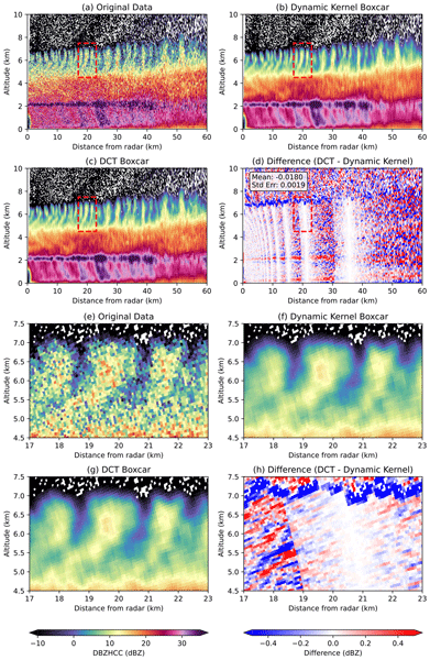
Real radar data typically suffers from issues such as beam blockage, attenuation, and removal of data points during quality control, leading to gaps in the observational field. Figure 4 demonstrates the application of the DCT method to C-band radar reflectivity data collected on 23 February 2022. The raw data (Fig. 4a) exhibits characteristic speckle noise. Even with a compact window size of 5 pixels, the method achieves substantial noise reduction while retaining feature definition. A notable implementation difference is that the spatial kernel (Fig. 4b) explicitly ignores NaN values, whereas the DCT method (Fig. 4c) requires a continuous field, handled here via linear interpolation. Despite this, the DCT approach, using a range-adaptive continuous boxcar window, effectively preserves mesoscale (1–2 km) features like cloud-top generating cells shown at cloud top in Fig. 4e–h, where sharp gradients are maintained against the noise floor, solving a common challenge where aggressive smoothing often washes out such fine structures.

Figure 4 Application to C-band radar observations on 23 February 2022 at 02:28 UTC. (a) Original observational field with noise and gaps. (b) Result of spatial dynamic kernel smoothing (window 5 pixels). (c) Result of DCT-based smoothing (analytical continuous boxcar, window 5 pixels). (d) Difference between spatial and spectral methods. The red dashed box indicates the zoom region shown in panels (e)–(h).

One caveat of the DCT method is that it requires a continuous data field without missing entries, and the present work fills gaps with linear interpolation prior to the DCT. Linear interpolation across a gap replaces the missing segment with a piecewise-linear bridge whose slope is unrelated to the underlying field, so two effects can bias the smoothed result. First, the bridge contributes a low-frequency trend across the gap; for gaps narrower than the local kernel width W this trend is small relative to the smoothing noise floor, but for wide gaps (large beam-blockage sectors, broad clutter removals) it can dominate the smoothed values within and near the gap. Second, the slope of the bridge generally differs from the local slope of the underlying field, producing a derivative discontinuity (a kink) at each gap boundary. The kink injects localized high-frequency content into the DCT spectrum; for W larger than the gap width this content is removed by the smoothing filter, but for narrow kernels residual kinks can survive as faint stripes parallel to the gap edge. The Astropy convolution-based interpolation (The Astropy Collaboration et al., 2022) is a robust drop-in upgrade that addresses both the low-frequency bias and the kink. More generally, support-normalized filtering (Knutsson and Westin, 1993; Westin et al., 1994; Pham et al., 2006), which avoids prefilling by treating missing entries as a separate certainty mask, has been developed by the authors as a methodological extension of the present framework (Valdivia-Prado et al., 2026).

The uniqueness of the DCT approach compared to other methods lies in its ability to leverage the separable convolution property even when the physical kernel size varies dynamically. In spatial domain methods, a range-dependent kernel requires recalculating window indices for every range bin, a process that breaks vectorization and incurs heavy branch prediction penalties inside nested loops. In contrast, the DCT method handles this complexity through simple element-wise matrix multiplication in the spectral domain, utilizing the analytical transfer function to represent the continuous variation of the kernel width. This separation of geometry (kernel definition) from computation (filtering) is the core advantage that distinguishes DCT from traditional spatial iterative methods, allowing it to scale entirely differently with problem size.

4 Performance Benchmarking and Efficiency Analysis

To evaluate the computational efficiency, we compared the DCT method against a typical spatial dynamic kernel implementation.

4.1 Experimental Setup

The benchmarks were conducted in two parts to isolate the effects of window size and total data volume:

• -

  Window Size Test. Performed using RHI radar observations with dimensions 474×1180 pixels (approx. 0.56 million pixels). Here, the window size was varied across $W\in \mathit{\{}\mathrm{5},\mathrm{9},\mathrm{15},\mathrm{31},\mathrm{51},\mathrm{101}\mathit{\}}$ pixels to capture the realistic overhead of handling jagged array edges and memory access patterns in operational data.

• -

  Data Size Test. Performed using a fixed window size of W=5 pixels across random noise arrays with dimensions representative of various operational scenarios:

  • -

    Small (100×500, 200×1000 pixels): Typical of single RHI scans or low-resolution grids.

  • -

    Medium (360×1500, 720×2500 pixels): Corresponding to standard PPI sweeps or single volume files.

  • -

    Large (7200×2500, 72 000× 2500 pixels): Representing aggregated datasets, such as a full volume scan or approximately 1 h of continuous volume data (up to 180 million pixels).

  This ensures a controlled environment to measure pure algorithmic scaling as a function of N.

4.2 Results

As shown in Fig. 5, the spatial convolution algorithm exhibits O(N⋅W²) complexity. Our benchmarks reveal that as the window size increases from 5–101 pixels, the execution time for the spatial dynamic kernel escalates drastically from 8.5 s to over 44 s. In sharp contrast, the DCT method's complexity is dominated by the O(Nlog N) transform step, making the smoothing operation effectively independent of window size. The analytical kernels (Gaussian and Analytical Boxcar) maintain a near-constant execution time of approximately 60 ms regardless of the filter width due to the analytical representation of the kernel (see Eqs. 7 and 18). This results in massive performance gains: for a large 101×101 pixels window, the Gaussian kernel achieves a speedup factor exceeding 800 times, and the Analytical Boxcar over 700 times. Even discrete DCT kernels like Savitzky–Golay and Hanning, which require iterative summation, outperform the spatial approach by factors of 60–100 times.

Figure 5 Computational benchmark results. (a) Execution time versus window size for a fixed data volume. (b) DCT speedup factors relative to the spatial dynamic kernel as a function of window size. (c) Execution time versus total number of pixels for a fixed window size. (d) DCT speedup factors as a function of total number of pixels.

The scalability analysis on dataset size further underscores the operational viability of the spectral approach. For a massive dataset representing approximately 1 h of volume data (180 million pixels), the spatial dynamic kernel required over 42 min (2518 s) to complete. The Gaussian DCT implementation processed the same volume in less than 12 s. This orders-of-magnitude improvement transforms computationally prohibitive geometric processing into a task feasible for real-time operational pipelines.

5 Discussion

Noise removal remains a critical challenge in scientific signal processing. In radar meteorology, noise manifests in diverse forms, ranging from ground clutter in the Doppler spectrum to thermal noise in $I/Q$ voltage data. This study specifically targets high-frequency fluctuations, or speckle, within moment data such as reflectivity. While we model this noise as randomly distributed and range-independent, the intrinsic polar geometry of radar data introduces a spatial dependency: data point density decreases inversely with range ($\mathrm{1}/r$). Consequently, scaling the smoothing window with range implies using fewer data points at longer distances, potentially compromising noise reduction efficacy. Given that the signal-to-noise ratio (SNR) typically degrades with range and beam broadening obscures fine-scale features, there is a theoretical basis for adaptive window scaling. Such an approach would need to balance noise suppression against the preservation of detectable spatial features. Within the present spectral framework, statistical adaptation is a natural direction: the analytical transfer function H[k] is an explicit object that can be modulated on a per-angle basis to widen or narrow the effective passband in regions of low or high local variance, respectively. Progress in this direction is already reported in the local-statistics extension of the present framework (Valdivia-Prado et al., 2026), which extends the present method to local statistics in polar coordinates through support-normalized filtering.

A common approach to denoising is to simply truncate high frequencies in the spectral domain, effectively applying an Ideal Low-Pass Filter. However, a hard cutoff in the frequency domain takes the shape of a boxcar function; by the convolution theorem, the inverse transform of this boxcar is a Sinc function ($\sin \left(x\right)/x$) in the spatial domain. The Sinc function is characterized by prominent oscillating tails, which manifest as spurious ringing artifacts near sharp signal transitions – a distinct error known as the Gibbs phenomenon (Gottlieb and Shu, 1997). Unlike the hard cutoff, the proposed DCT method multiplies the spectrum by a smooth shaping function (e.g., Gaussian or Hanning, as shown in Eq. 6), which decays gradually. This avoids the abrupt spectral discontinuity that causes the spatial ringing, effectively preserving the monotonicity of step-like features. Furthermore, the DCT's implicit even symmetry at boundaries significantly reduces edge artifacts compared to the DFT (FFT), which assumes periodic boundaries (Ahmed et al., 1974; Makhoul, 1980). This property is a primary reason why DCT is the standard for image compression algorithms like JPEG (ITU-T, 1992). To visualize the Gibbs phenomenon, Fig. 6 presents a comparison between an Ideal Low-Pass filter (which causes ringing) and the proposed DCT smoothing. The sharp cutoff in the frequency domain for the low-pass filter creates oscillations in the spatial domain near discontinuities. The DCT method, using a smooth Gaussian-like transfer function, avoids this issue entirely, preserving the monotonicity of the step function without artificial ringing.

Figure 6 Illustration of the Gibbs phenomenon. (a) Reconstructed signal comparison: an ideal low-pass filter (red line) produces ringing artifacts (Gibbs effect) near sharp transitions, whereas the DCT-based smoothing with a continuous Gaussian taper (blue line) provides a clean, physically consistent result compared to the reference signal (dashed black). (b) Corresponding DCT spectral domain visualization showing the hard cut vs. the smooth Gaussian weighting.

The Gibbs phenomenon will behave differently on different radar variables. While this study focused on reflectivity (Z_e), the DCT smoothing method is applicable to all radar moments, provided their physical characteristics are respected. Doppler velocity presents a unique challenge due to aliasing, where the velocity value wraps around the Nyquist interval (e.g., jumping from +V_max to −V_max), creating sharp, artificial discontinuities. Smoothing across these folded boundaries is problematic because it mathematically averages physically disparate velocities (e.g., averaging +15 and −15 to 0 m s⁻¹), and the extreme artificial gradients at the fold trigger severe Gibbs ringing if not handled correctly. Consequently, velocity unfolding (de-aliasing) is a strict prerequisite for spectral smoothing to ensure the underlying field is continuous and physically meaningful before the transform is applied. For differential reflectivity (Z_dr) and differential phase (ϕ_dp), the smoothing process is identical to that of reflectivity. Furthermore, this technique could be advantageous for estimating the specific differential phase (K_dp), which typically requires substantial smoothing to mitigate noise. However, for correlation coefficient (ρ_hv), care must be taken to ensure smoothed values remain within the valid [0, 1] interval, although a normalized convolution naturally preserves the convex hull of the data.

While the Fast Fourier Transform (FFT) is often the default choice for spectral convolution, the DCT offers distinct advantages for real-valued radar data. Since the DCT involves only real arithmetic, it avoids the storage and computation overhead of complex numbers inherent to the FFT. This results in faster execution and simpler implementation, as supported by the benchmarks (Sect. 4) and literature (Makhoul, 1980).

For general-purpose range-dependent smoothing of polar radar data we recommend the analytical continuous Gaussian kernel (Eq. 18) as the default: it provides the smoothest taper (no spectral sidelobes, no ringing), it allows the fractional pixel widths required by the $\mathrm{1}/r$ angular geometry, and its performance is superior. The analytical continuous boxcar (Eq. 7) is the appropriate choice when a hard cutoff kernel is desired, while the discrete boxcar (Eq. 4) should be reserved for cases that require an integer kernel width matching a spatial reference. The Savitzky–Golay kernel (Eq. 19) preserves low-order polynomial features such as the peak and area of reflectivity cores and is worth exploiting further in the present framework; its coefficients depend only on the window width W and the polynomial order p (not on the data values), are pre-computed once from the polynomial basis, and are applied as a fixed-weight FIR filter with the same O(W) per-pixel cost as any other kernel in this paper. Window families that are common in other application domains, such as the Hamming, Blackman, Tukey, Kaiser, and Welch windows (Blackman and Tukey, 1959; Harris, 1978; Kaiser, 1966; Welch, 1967), are not the focus of the present study.

6 Conclusions

We have presented a comprehensive method for smoothing polarimetric radar data using the Discrete Cosine Transform. By deriving the analytical transfer function for continuous kernels and formulating the 2D range-dependent convolution in the spectral domain, we achieved a method that is both physically consistent and computationally superior to spatial domain alternatives.

The primary contribution of this work is the resolution of the conflict between geometric accuracy and computational efficiency. Traditional spatial methods require O(N⋅W²) operations, meaning the computational cost explodes as the smoothing window W increases to match beam broadening at long ranges. In contrast, the DCT method operates in O(Nlog N) time, rendering the processing time effectively independent of the kernel size.

Our performance benchmarks demonstrate that this theoretical advantage translates into massive operational gains:

1. Kernel Scalability. For large smoothing windows (e.g., 101 pixels), the analytical DCT kernels (Gaussian and Boxcar) provided speedup factors exceeding 800 times compared to the spatial dynamic kernel.

2. Data Volume Scalability. For a dataset representing approximately 1 h of continuous volume scans (180 million pixels), the spatial algorithm required over 42 min (2518 s) to complete. The DCT implementation processed the same volume in less than 12 s.

This orders-of-magnitude improvement reduces hours of processing time to seconds. Complex geometric corrections that were previously computationally prohibitive can now be integrated into standard operational pipelines with negligible latency.

While the method requires a continuous data field, necessitating a preprocessing step to interpolate gaps (e.g., removed clutter or beam blockage), the resulting low-frequency bias and gap-edge kinks are bounded for gap widths smaller than the local kernel and can be eliminated by the support-normalized extension developed by the authors (Valdivia-Prado et al., 2026). The DCT approach avoids the Gibbs phenomenon associated with the Ideal Low-Pass Filter discussed in Sect. 5 and preserves the convex hull of the data, making it safe for variables such as correlation coefficient (ρ_hv). For Doppler velocity, de-aliasing is a strict prerequisite: the wrapped-velocity fold is an artificial discontinuity that the spectral transform will treat as a sharp physical edge and propagate as ringing. Overall, this spectral framework offers a robust, high-performance standard for modern weather radar analysis.