Importance of subpixel Earth surface reflectance and altitude for atmospheric trace gas retrievals from passive satellite instruments

Satellite retrievals of atmospheric greenhouse gas columns are used to obtain information about greenhouse gas sources and sinks by inverse modeling. Such an application requires high accuracy, as even small biases of the retrieved concentrations may result in large errors of the inferred rates of surface emissions (source) and deposition, surface uptake or removal in the atmosphere (sinks). For example, for the upcoming satellite mission dedicated to carbon dioxide monitoring (CO2M), co-funded by ESA and the European Commission for the Copernicus Programme, the accuracy of the column-averaged dry-air mole fraction of carbon dioxide (XCO₂) is required to be better than 0.5 ppm. Here we investigate a potentially important systematic error source, namely XCO₂ biases due to correlated sub-pixel variability of surface reflectance (abbreviated as albedo) and altitude. To minimize this error source we propose the use of an albedo-weighted surface altitude which better represents the satellite's spatial sample than the unweighted average by using a linearized theoretical analysis at one wavelength with many assumptions including a non-scattering atmosphere and neglecting the influences of different illumination of the detector pixel (the point spread function) and effects of the bidirectional reflectance distribution function. We use Copernicus Sentinel-2 data combined with Copernicus Digital Elevation Model (DEM) data and the Fast atmOspheric traCe gAs retrievaL (FOCAL) algorithm and create a variety of self-consistent experiments to test this theory. First, we conduct experiments with defined conditions and second, we apply the methodology to some real-world examples: the Bełchatów power plant in Poland, the Black Forest in Germany, the region around Mont Blanc in the European Alps and the whole country of Germany. In all these examples, we find that using the albedo-weighted average of the surface altitude reduces biases at locations with heterogeneous surface structure. In addition, we developed a possible post-processing equation to account for this process, because high-resolution albedo currently is not measured simultaneously with satellite instruments. We also find that filter parameters connected to the surface roughness might be relaxed when using the albedo-weighted surface altitude in the retrievals. Furthermore, we examine the dependence of the XCO₂ errors on the size of the spatial samples and find that the errors become larger with larger spatial samples, but are generally smaller by more than a factor of four when using the albedo-weighted instead of the unweighted average of the surface altitude. In conclusion, we show that the use of the albedo-weighted surface altitude in the retrieval process results in significant reduction of the XCO₂ bias in these self-consistent experiments compared to the use of the unweighted mean altitude, as currently used in most retrieval schemes.

1 Introduction

Accurate measurements of greenhouse gases (GHGs) are crucial to understand ongoing changes in the climate system due to human influence and to develop mitigation strategies (IPCC, 2023). Greenhouse gas column-averaged measurements retrieved from observations of spectrometers on orbiting satellite platforms complement the sparse but very accurate in situ and ground-based passive remote sensing measurements of GHGs such that the combined data yield potentially accurate and consistent global datasets. In order to estimate the large-scale natural occurring and human modified sources and sinks, upcoming satellite missions, such as the European Space Agency (ESA) and European Commission funded Copernicus mission for carbon dioxide monitoring (CO2M), have stringent requirements for accuracy and precision for retrievals of the column-averaged dry-air mole fraction of carbon dioxide (XCO₂). For instance, CO2M requires systematic errors to be smaller than 0.5 ppm and random errors to be smaller than 0.7 ppm for a given observation scenario (ESA, 2020).

Following on the pioneering development of the SCanning Imaging Absorption spectroMeter for Atmospheric CHartographY (SCIAMACHY), the retrieval of XCO₂ from the measurements of space-based passive remote sensing spectrometers observing in the near-infrared (NIR) and short-wave infrared (SWIR) have become a successful and common measurement strategy. Such instruments measure in near nadir geometry (looking downwards directly to Earth's surface). This enables the determination of GHG absorption along the electromagnetic solar radiation path through the atmosphere (called light path hereafter), which is reflected at the Earth's surface before upwelling to the satellite. Subsequently or simultaneously combining a knowledge of the light path, the XCO₂ is then estimated (Burrows et al., 1995; Bovensmann et al., 1999; Buchwitz et al., 2005; Kuze et al., 2009; Reuter et al., 2010; Schneising et al., 2011; Nakajima et al., 2012; Crisp, 2015; Liu et al., 2018; Taylor et al., 2020). Electromagnetic radiation upwelling to the top of the atmosphere comprises both surface scattering and scattering within the atmosphere by gases, aerosol and clouds. For cloud-free ground scenes, which are usually preferred for the determination and analysis of XCO₂, different algorithms use different approaches to account for and separate the impacts of these two sources of electromagnetic radiation measured by the satellite spectrometers, which have different XCO₂ values. Consequently, the exact knowledge of the length of the light path is crucial to meet the requirements for accuracy and precision (Hachmeister et al., 2022).

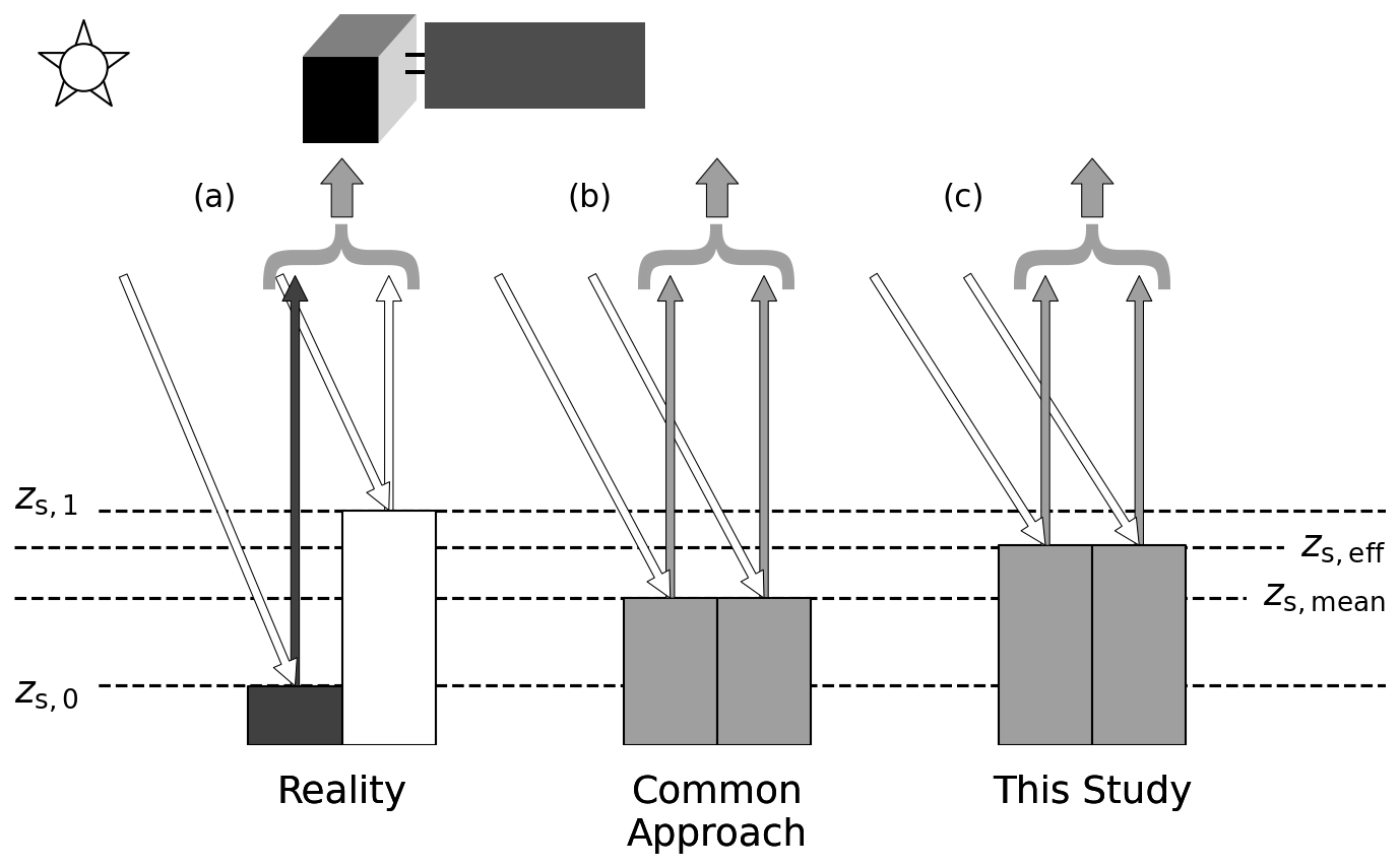
Figure 1 Theoretical example where (a) a spatial sample is split into two halves with an albedo of 0.25 and z_s,0 in one half and an albedo of one (perfect reflector) and a surface altitude $z_{\mathrm{s},\mathrm{1}}>z_{\mathrm{s},\mathrm{0}}$ in the other half and (b) the assumptions made in common greenhouse gas retrieval algorithms and (c) the corrected surface altitude suggested by this study. The surface altitude is used to compute the dry-air column from external data, which is in the denominator of XCO₂ and XCH₄.

XCO₂ is defined as the CO₂ column divided by the dry-air column. The dry-air column derived from the length of the light path neglecting atmospheric scattering effects depends on the atmospheric state, but especially also on the altitude of the scattering surface. If the surface altitude is assumed to be too low (see Fig. 1, panel b compared to panel c), the light path will be longer than the real light path and the dry-air column is overestimated. Therefore, the retrieved XCO₂ will be too low compared to the real XCO₂ and vice versa. Thus, errors in the surface altitude have direct impact on the XCO₂ error if the surface pressure is not a retrieved parameter. This is a potential systematic error source which should be avoided in trace gas retrievals.

Changes in XCO₂ should be proportional to the relative changes in the surface pressure because the dry-air column is proportional to the surface pressure, i.e. a 1 % change in surface pressure will lead to a 1 % error in XCO₂ when ignoring pressure broadening of the absorption lines. Around sea level, a pressure change of 1 hPa (which is about 0.1 % of the air column) corresponds roughly to a change in altitude of 10 m. Considering a background value of about XCO₂=419 ppm (global value of 2023, Copernicus Climate Change Service, 2024), this leads to an approximate dependence of 0.04 ppm m⁻¹.

Spatial samples of satellite instruments have a ground scene spatial resolution, e.g. 1.8 × 2.2 km² for CO2M (ESA, 2020). Thus, assumptions have to be made about the subpixel surface altitude and reflectance which are representative for the spatial sample of the satellite. A common assumption in trace gas retrievals is to use the average surface altitude (Degünther et al., 1998; Butz et al., 2011; Cogan et al., 2012; Reuter et al., 2017a; Noël et al., 2021; Schneising et al., 2023) or to use for instance the center altitude which is assumed to be representative for the spatial sample (e.g., Wang et al., 2008; Ohyama et al., 2012). This is a good assumption for homogeneous scenes where altitude variation is small and, accordingly, screening for surface roughness is one of the steps in greenhouse gas retrievals' pre- or post-processing (e.g., Cogan et al., 2012; Reuter et al., 2017a).

A theoretical example illustrating how correlated heterogeneity in surface reflectance (called albedo in the remaining part of this study) and altitude leads to errors when using the average surface altitude is shown in Fig. 1, where the spatial sample of a satellite is split into two halves, with an albedo of 0.25 in the first half and an albedo of one in the second half. In addition, there is an altitude change from lower altitude z_s,0 to a higher altitude z_s,1. The common approach to compute the surface altitude for the spatial sample is to use the unweighted average of the subpixel altitude values z_s,mean (Fig. 1b). On the other hand, in the ideal case without scattering, the major signal arriving at the satellite's detector comes from the bright half with altitude z_s,1. Therefore, the surface altitude which is representative for the two occurring light paths, denoted by z_s,eff, is close to z_s,1 (panel c) whereas the average is lower (panel b). In conclusion, this example shows that a more sophisticated approach including information of subpixel surface altitude and albedo is needed to compute the representative surface altitude for the light path in the satellite's spatial sample. Here, as in the remaining part of this study, we neglect effects due to the point spread function or the bidirectional reflectance distribution function.

While heterogeneity in subpixel surface reflectance and subpixel topography has been investigated in many studies separately (e.g., Shepherd and Dymond, 2003; Roupioz et al., 2014), the examination of the combined effect of both heterogeneous surface albedo and altitude is missing so far and is the subject of this study.

As a test case for this study, we use the future CO2M mission which is dedicated to CO₂ monitoring. It will be launched into a near-polar sun-synchronous orbit with an equator crossing time at 11:30 LT in a descending mode where the first of three satellites is expected to be launched in 2027 (Janssens-Maenhout et al., 2020; Sierk et al., 2021; Meijer et al., 2023). The CarbonSat concept is the basis for this mission with extended instrumentation (Bovensmann et al., 2010; Velazco et al., 2011; Buchwitz et al., 2013; Pillai et al., 2016; Broquet et al., 2018). A push-broom imaging spectrometer (CO2I) measuring solar radiances reflected at the Earth's surface and scattered in the atmosphere in three spectral bands is the primary instrument on CO2M, measuring in (1) the near infrared (NIR, 747–773 nm), used to retrieve information about scattering properties and the atmospheric dry-air column density, aerosols and solar-induced fluorescence (SIF); and (2) two bands in the short-wave infrared (SWIR1, 1590–1675 and SWIR2, 1990–2095 nm), used to derive information about atmospheric CO₂, CH₄, aerosols and water vapor. Accordingly, XCO₂ and XCH₄ can be determined from these measurements. The expected across-track 110 spatial samples of CO2M will have a spatial resolution of $\sim \mathrm{1.8}\times \mathrm{2.2}$ km² on the ground with a swath width of about 250 km. Additional instruments are a spectrometer measuring in the visible spectral range for NO₂ measurements (NO2I), a Multi-Angle Polarimeter (MAP) primarily for aerosols and a Cloud Imager (CLIM), see also Meijer et al. (2023) for an overview.

It should be noted that there are approaches to simultaneously retrieve the surface pressure using the NIR band of GHG satellites (e.g., Reuter et al., 2010; O'Dell et al., 2018; Jacobs et al., 2024) which will then account for part of the surface altitude change due to the albedo if the albedo behaves the same way in the SWIR CO₂ bands, which is not always the case.

As the trace gas concentrations are usually retrieved from measurements in multiple spectral windows (NIR, SWIR1 and SWIR2 in the case of CO₂), it is important to note that the surface reflectance (albedo) depends on the wavelength, i.e. the albedo is different for each spectral pixel of the detector, but especially between the wavelength bands. For example, it could happen that the bright part in Fig. 1a is in the other half for another spectral window so that the altitude to be used there should be close to z_s,0.

In this study, we introduce both (1) an approach for how to account for the effect of the albedo-weighted averaged surface altitude directly in the retrieval algorithms, which depends on the simultaneous measurements of the surface albedo, as discussed below, and (2) a possible post-processing correction for this effect if measurements of the subpixel albedo are not available simultaneously. We neglect the spectral dependence of the albedo within a given wavelength band in this study and account for the differences in albedo amongst different wavelength bands, only. We motivate in Sect. 2 with a theoretical derivation that the albedo-weighted average of the surface altitude is a result of a simplified radiative transfer scenario. We then describe the datasets and methods used to account for this effect with the retrieval algorithm FOCAL-CO2M in Sect. 3. We then apply this method to idealized test cases and real orography in Sect. 4, where we also derive a possible post-processing algorithm that can be used to apply a correction for XCO₂ after running the retrieval. We finish with concluding remarks in Sect. 5.

2 Albedo-weighted average of surface altitude

Satellite instruments using the Earth's surface as reflecting surface measure the average radiance at a given wavelength from a spatial sample on the Earth's surface of a given size (2.2×1.8 km² for CO2M). We assume in this study that the spatial sample has the exact size as given by the boundaries of the CO2M simulated orbits and that the detector pixel is illuminated homogeneously, which, in general, is not the case in reality (e.g., Sierk et al., 2021). In order to account for the subpixel heterogeneity, we divide this spatial sample into n fully homogeneous subpixels with known subpixel dry-air column d_i and subpixel surface albedo α_i. By assuming only gaseous absorption in a non-scattering isothermal atmosphere and neglecting the pressure dependence of the molecular cross section σ, gravity acceleration g and dry-air column-averaged mole fraction c of the absorbing species, this can be described by the Lambert-Beer law for an absorbing wavelength as follows:

$$\begin{array}{}\text{(1)}& I_{\mathrm{sub}}=I_{\mathrm{0}}{\displaystyle \frac{\mathrm{1}}{n}}\sum _{i=\mathrm{1}}^n{\mathit{\alpha }}_i\exp \left(-F_{\mathrm{air}}{d}_i\mathit{\sigma }c\right),\end{array}$$

where I₀ is the reflected radiance without absorption and an albedo of one (perfect reflector). The air mass factor F_air converts the measured slanted air column to a vertical air column and depends on the solar and satellite viewing angles (e.g., McGarragh et al., 2024) which can be assumed to be constant within the spatial sample. In nadir geometry and for a solar zenith angle of 0°, F_air=2 because the sunlight has to go through the atmosphere twice before it arrives at the detector. It is assumed that c is independent of the surface altitude within the single satellite spatial sample since the mole fraction does not depend on the air density.

We aim to determine the effective dry-air column which represents the light path in the spatial sample of the measurement, which can then be written according to the Lambert-Beer law with an effective surface albedo α_eff and an effective dry-air column d_eff:

$$\begin{array}{}\text{(2)}& I_{\mathrm{eff}}=I_{\mathrm{0}}{\mathit{\alpha }}_{\mathrm{eff}}\exp \left(-F_{\mathrm{air}}{d}_{\mathrm{eff}}\mathit{\sigma }c\right).\end{array}$$

The radiances I_sub and I_eff should be the same, therefore we set $I_{\mathrm{sub}}\stackrel{!}{=}{I}_{\mathrm{eff}}$:

$$\begin{array}{}\text{(3)}& I_{\mathrm{0}}{\mathit{\alpha }}_{\mathrm{eff}}\exp \left(-F_{\mathrm{air}}{d}_{\mathrm{eff}}\mathit{\sigma }c\right)=I_{\mathrm{0}}{\displaystyle \frac{\mathrm{1}}{n}}\sum _{i=\mathrm{1}}^n{\mathit{\alpha }}_i\exp \left(-F_{\mathrm{air}}{d}_i\mathit{\sigma }c\right).\end{array}$$

The goal is to derive an expression for d_eff depending on the known subpixel albedo and dry-air column values from this equation and then use the dependence of d_eff on the surface altitude to get an expression of the surface altitude in the end. In order to keep the validity of Eq. (3) for c=0 (no absorption) or σ=0 (no absorption at non-absorbing wavelength), the effective albedo α_eff is the average of the subpixel albedo values:

$$\begin{array}{}\text{(4)}& {\mathit{\alpha }}_{\mathrm{eff}}={\displaystyle \frac{{\sum }_{i=\mathrm{1}}^n{\mathit{\alpha }}_i}{n}}.\end{array}$$

Inserting Eq. (4) in Eq. (3) yields:

$$\begin{array}{}\text{(5)}& \begin{array}{rl}{I}_{\mathrm{0}}& {\displaystyle \frac{\mathrm{1}}{n}}\sum _{i=\mathrm{1}}^n{\mathit{\alpha }}_i\exp \left(-F_{\mathrm{air}}{d}_{\mathrm{eff}}\mathit{\sigma }c\right)\\ & =I_{\mathrm{0}}{\displaystyle \frac{\mathrm{1}}{n}}\sum _{i=\mathrm{1}}^n{\mathit{\alpha }}_i\exp \left(-F_{\mathrm{air}}{d}_i\mathit{\sigma }c\right).\end{array}\end{array}$$

Solving for d_eff yields:

$$\begin{array}{}\text{(6)}& d_{\mathrm{eff}}=-{\displaystyle \frac{\mathrm{1}}{F_{\mathrm{air}}\mathit{\sigma }c}}\ln \left[{\displaystyle \frac{{\sum }_{i=\mathrm{1}}^n{\mathit{\alpha }}_i\exp \left(-F_{\mathrm{air}}{d}_i\mathit{\sigma }c\right)}{{\sum }_{i=\mathrm{1}}^n{\mathit{\alpha }}_i}}\right].\end{array}$$

In general, the dry-air column d is the integral of the air density ρ from the surface altitude z_s to infinity (where the density is zero):

$$\begin{array}{}\text{(7)}& d={\displaystyle \frac{N_{\mathrm{A}}}{M_{\mathrm{air}}}}\underset{z_{\mathrm{s}}}{\overset{\mathrm{\infty }}{\int }}\mathit{\rho }\left(z\right)\mathrm{d}z\end{array}$$

with N_A the Avogadro constant and M_air the molar mass of dry air. In the isothermal atmosphere with temperature $\stackrel{\mathrm{‾}}{T}$, ρ(z) can be calculated with the hydrostatic approximation:

$$\begin{array}{}\text{(8)}& \mathit{\rho }\left(z\right)={\mathit{\rho }}_{\mathrm{0}}\exp \left(-{\displaystyle \frac{z}{H}}\right)\end{array}$$

with $H=R\stackrel{\mathrm{‾}}{T}/g$ and the specific gas constant of dry air R and the gravitational acceleration g. Inserting Eq. (8) in Eq. (7) yields:

$$\begin{array}{}\text{(9)}& d={\displaystyle \frac{{\mathit{\rho }}_{\mathrm{0}}{N}_{\mathrm{A}}}{M_{\mathrm{air}}}}\underset{{\mathrm{z}}_{\mathrm{s}}}{\overset{\mathrm{\infty }}{\int }}\exp \left(-{\displaystyle \frac{z}{H}}\right)\mathrm{d}z=d_{\mathrm{0}}\exp \left(-{\displaystyle \frac{z_{\mathrm{s}}}{H}}\right)\end{array}$$

with $d_{\mathrm{0}}=\frac{{\mathit{\rho }}_{\mathrm{0}}H{N}_{\mathrm{A}}}{M_{\mathrm{air}}}$. Thus, the dry-air column depends exponentially on the surface altitude. In the retrieval, it will be assumed that the spatial sample is homogeneous so that Eq. (9) is applicable to the effective dry-air column as well, providing the effective surface altitude z_s,eff, which is representative for light path in the satellite's spatial sample. Thus, inserting Eq. (9) in Eq. (6) yields

$$\begin{array}{}\text{(10)}& \begin{array}{rl}{d}_{\mathrm{0}}& \exp \left(-{\displaystyle \frac{z_{\mathrm{s},\mathrm{eff}}}{H}}\right)=\\ & -{\displaystyle \frac{\mathrm{1}}{F_{\mathrm{air}}\mathit{\sigma }c}}\ln \left[{\displaystyle \frac{{\sum }_{i=\mathrm{1}}^n{\mathit{\alpha }}_i\exp \left(-d_{\mathrm{0}}\exp \left(-z_{\mathrm{s},i}/H\right)F_{\mathrm{air}}\mathit{\sigma }c\right)}{{\sum }_{i=\mathrm{1}}^n{\mathit{\alpha }}_i}}\right].\end{array}\end{array}$$

Solving for the effective altitude z_s,eff and defining the constant τ₀≡F_aird₀σc, which is the optical thickness of the absorption by the species as if the surface altitude was 0 m, leads to the following equation:

$$\begin{array}{}\text{(11)}& \begin{array}{rl}{z}_{\mathrm{s},\mathrm{eff}}& \left({\mathit{z}}_{\mathrm{s}}\right)=\\ & -H\ln \left(-{\displaystyle \frac{\mathrm{1}}{{\mathit{\tau }}_{\mathrm{0}}}}\ln \left[{\displaystyle \frac{{\sum }_{i=\mathrm{1}}^n{\mathit{\alpha }}_i\exp \left(-{\mathit{\tau }}_{\mathrm{0}}\exp \left(-z_{\mathrm{s},i}/H\right)\right)}{{\sum }_{i=\mathrm{1}}^n{\mathit{\alpha }}_i}}\right]\right).\end{array}\end{array}$$

Here, ${\mathit{z}}_{\mathrm{s}}=(z_{\mathrm{s},\mathrm{1}},z_{\mathrm{s},\mathrm{2}},\mathrm{\dots },z_{\mathrm{s},n}{)}^T$ is an n-dimensional vector consisting of the subpixel surface altitudes. Hence, the effective surface altitude depends on the individual subpixel altitudes by the sum of two exponentials included in two logarithms. We further apply a n-dimensional Taylor expansion of first order to this function. The Taylor expansion uses the derivative of Eq. (11) for each z_s,i. It is based around the pixel average surface altitude z_s,mean which results in all subpixel altitudes z_s,i equal z_s,mean at the expansion point, denoted as ${\mathit{z}}_{\mathrm{s}}={\mathit{z}}_{\mathrm{s},\mathrm{mean}}=(z_{\mathrm{s},\mathrm{mean}},\mathrm{\dots },z_{\mathrm{s},\mathrm{mean}}{)}^T$ in the following. We use the average because the differences of the individual z_s,i values from the average is assumed to be small enough to apply a Taylor expansion of first order. The differences should then also be usable independent of the absolute value of the average altitude, see discussion later in this section. Note also that we do not apply any restrictions to z_s,mean, except that the difference to z_s,i is small enough, so that z_s,mean could also be any value of surface altitude that has been used in the retrieval. To simplify the notation, we define

$$\begin{array}{}\text{(12)}& {\displaystyle }L\left(z_{\mathrm{s},i}\right)\equiv \exp (-{\mathit{\tau }}_{\mathrm{0}}\exp (-z_{\mathrm{s},i}/H\left)\right),\text{(13)}& {\displaystyle }h\left({\mathit{z}}_{\mathrm{s}}\right)\equiv {\displaystyle \frac{{\sum }_{i=\mathrm{1}}^n{\mathit{\alpha }}_{i}L\left(z_{\mathrm{s},i}\right)}{{\sum }_{i=\mathrm{1}}^n{\mathit{\alpha }}_i}}\text{(14)}& {\displaystyle }w\left({\mathit{z}}_{\mathrm{s}}\right)\equiv -{\displaystyle \frac{\mathrm{1}}{{\mathit{\tau }}_{\mathrm{0}}}}\ln \left[h\left({\mathit{z}}_{\mathrm{s}}\right)\right]\text{(15)}& {\displaystyle }{z}_{\mathrm{s},\mathrm{eff}}\left({\mathit{z}}_{\mathrm{s}}\right)=-H\ln \left(w\left({\mathit{z}}_{\mathrm{s}}\right)\right),\end{array}$$

so that the derivative of z_s,eff with respect to one subpixel z_s,j can be written as:

$$\begin{array}{}\text{(16)}& {\displaystyle \frac{\partial z_{\mathrm{s},\mathrm{eff}}\left({\mathit{z}}_{\mathrm{s}}\right)}{\partial z_{\mathrm{s},j}}}={\displaystyle \frac{\partial z\left({\mathit{z}}_{\mathrm{s}}\right)}{\partial w\left({\mathit{z}}_{\mathrm{s}}\right)}}{\displaystyle \frac{\partial w\left({\mathit{z}}_{\mathrm{s}}\right)}{\partial h\left({\mathit{z}}_{\mathrm{s}}\right)}}{\displaystyle \frac{\partial h\left({\mathit{z}}_{\mathrm{s}}\right)}{\partial L\left(z_{\mathrm{s},j}\right)}}{\displaystyle \frac{\partial L\left(z_{\mathrm{s},j}\right)}{\partial z_{\mathrm{s},j}}}\end{array}$$

which is evaluated at ${\mathit{z}}_{\mathrm{s}}={\mathit{z}}_{\mathrm{s},\mathrm{mean}}$ for the Taylor expansion. We get

$$\begin{array}{}\text{(17)}& \begin{array}{rl}& {\left.{\displaystyle \frac{\partial z_{\mathrm{s},\mathrm{eff}}\left({\mathit{z}}_{\mathrm{s}}\right)}{\partial w\left({\mathit{z}}_{\mathrm{s}}\right)}}\right|}_{{\mathit{z}}_{\mathrm{s}}={\mathit{z}}_{\mathrm{s},\mathrm{mean}}}\\ & ={\left.-H{\displaystyle \frac{\mathrm{1}}{-\frac{\mathrm{1}}{{\mathit{\tau }}_{\mathrm{0}}}\ln \left[\frac{{\sum }_{i=\mathrm{1}}^n{\mathit{\alpha }}_i\exp (-{\mathit{\tau }}_{\mathrm{0}}\exp (-z_i/H\left)\right)}{{\sum }_{i=\mathrm{1}}^n{\mathit{\alpha }}_i}\right]}}\right|}_{{\mathit{z}}_{\mathrm{s}}={\mathit{z}}_{\mathrm{s},\mathrm{mean}}}\\ & =-H\exp \left(+{\displaystyle \frac{z_{\mathrm{s},\mathrm{mean}}}{H}}\right)\end{array}\end{array}$$

and

$$\begin{array}{}\text{(18)}& \begin{array}{rl}& {\left.{\displaystyle \frac{\partial w\left({\mathit{z}}_{\mathrm{s}}\right)}{\partial h\left({\mathit{z}}_{\mathrm{s}}\right)}}\right|}_{{\mathit{z}}_{\mathrm{s}}={\mathit{z}}_{\mathrm{s},\mathrm{mean}}}={\left.-{\displaystyle \frac{\mathrm{1}}{{\mathit{\tau }}_{\mathrm{0}}}}{\displaystyle \frac{{\sum }_{i=\mathrm{1}}^n{\mathit{\alpha }}_i}{{\sum }_{i=\mathrm{1}}^n{\mathit{\alpha }}_{i}L\left(z_i\right)}}\right|}_{{\mathit{z}}_{\mathrm{s}}={\mathit{z}}_{\mathrm{s},\mathrm{mean}}}\\ & =-{\displaystyle \frac{\mathrm{1}}{{\mathit{\tau }}_{\mathrm{0}}}}{\displaystyle \frac{\mathrm{1}}{L\left(z_{\mathrm{s},\mathrm{mean}}\right)}}\end{array}\end{array}$$

and

$$\begin{array}{}\text{(19)}& {\left.{\displaystyle \frac{\partial h\left({\mathit{z}}_{\mathrm{s}}\right)}{\partial L\left(z_{\mathrm{s},j}\right)}}\right|}_{{\mathit{z}}_{\mathrm{s}}={\mathit{z}}_{\mathrm{s},\mathrm{mean}}}={\displaystyle \frac{{\mathit{\alpha }}_j}{{\sum }_{i=\mathrm{1}}^n{\mathit{\alpha }}_i}}\end{array}$$

and

$$\begin{array}{}\text{(20)}& \begin{array}{rl}& {\left.{\displaystyle \frac{\partial L\left(z_{\mathrm{s},j}\right)}{\partial z_{\mathrm{s},j}}}\right|}_{{\mathit{z}}_{\mathrm{s}}={\mathit{z}}_{\mathrm{s},\mathrm{mean}}}\\ & ={\left.L\left(z_{\mathrm{s},j}\right)\cdot (-{\mathit{\tau }}_{\mathrm{0}})\cdot \exp (-z_{\mathrm{s},j}/H)\cdot (-{\displaystyle \frac{\mathrm{1}}{H}})\right|}_{{\mathit{z}}_{\mathrm{s}}={\mathit{z}}_{\mathrm{s},\mathrm{mean}}}\\ & =L\left(z_{\mathrm{s},\mathrm{mean}}\right)\cdot (-{\mathit{\tau }}_{\mathrm{0}})\cdot \exp (-z_{\mathrm{s},\mathrm{mean}}/H)\cdot (-{\displaystyle \frac{\mathrm{1}}{H}}).\end{array}\end{array}$$

As can be seen, all terms of Eq. (20) cancel with the results of Eqs. (17) and (18), so that Eq. (16) simplifies to:

$$\begin{array}{}\text{(21)}& {\left.{\displaystyle \frac{\partial z_{\mathrm{s},\mathrm{eff}}\left({\mathit{z}}_{\mathrm{s}}\right)}{\partial z_{\mathrm{s},j}}}\right|}_{{\mathit{z}}_{\mathrm{s}}={\mathit{z}}_{\mathrm{s},\mathrm{mean}}}={\displaystyle \frac{{\mathit{\alpha }}_j}{{\sum }_{i=\mathrm{1}}^n{\mathit{\alpha }}_i}}.\end{array}$$

The n-dimensional Taylor expansion in first order around z_s,mean can then be written as:

$$\begin{array}{}\text{(22)}& \begin{array}{rl}{z}_{\mathrm{s},\mathrm{eff}}& \left({\mathit{z}}_{\mathrm{s}}\right)\approx z_{\mathrm{s},\mathrm{eff},\mathrm{Taylor}}\left({\mathit{z}}_{\mathrm{s}}\right)=\\ & z_{\mathrm{s},\mathrm{mean}}+\sum _{j=\mathrm{1}}^n{\left.{\displaystyle \frac{\partial z\left({\mathit{z}}_{\mathrm{s}}\right)}{\partial z_{\mathrm{s},j}}}\right|}_{{\mathit{z}}_{\mathrm{s}}={\mathit{z}}_{\mathrm{s},\mathrm{mean}}}(z_{\mathrm{s},j}-z_{\mathrm{s},\mathrm{mean}})\end{array}\end{array}$$

which results in the albedo-weighted average of the surface altitude:

$$\begin{array}{}\text{(23)}& z_{\mathrm{s},\mathrm{eff},\mathrm{Taylor}}\left({\mathit{z}}_{\mathrm{s}}\right)={\displaystyle \frac{{\sum }_{i=\mathrm{1}}^n{\mathit{\alpha }}_i{z}_{\mathrm{s},i}}{{\sum }_{i=\mathrm{1}}^n{\mathit{\alpha }}_i}}\equiv z_{\mathrm{s},\mathrm{weighted}}\left({\mathit{z}}_{\mathrm{s}}\right).\end{array}$$

The question remains under which conditions this first-order Taylor approximation is valid. However, an evaluation using Eqs. (11) and (23) will not help in the real application because the derivation is based on a one-wavelength retrieval while real retrievals use many wavelengths of different wavelength bands to retrieve the greenhouse gas concentration. We analyzed the parameter τ₀ for all wavelengths used in the retrieval for CO2M, see Sect. 3.3, and found that it covers four orders of magnitude ranging from values between 0.008 and 25.6. This leads to errors due to this first-order approximation also differing by several orders of magnitude (not shown). As it cannot be evaluated in advance of the retrieval which will be the dominant error cause, this derivation is a demonstration that the albedo-weighted average of the surface altitude is a direct result of the assumptions made in this section, but its value for applications in actual retrievals is yet to be shown. This is why we start with examples with well-defined conditions increasing the complexity of the underlying data and finish with applications using real subpixel albedo and altitude data in the first part of the results section (Sect. 4).

The effective altitude that represents the light path and which is therefore to be used internally for trace gas retrievals has to account for the subpixel albedo, which will be further analyzed in various examples in the following sections. It should be noted that the albedo is dependent on the wavelength and it is expected that the effective altitudes for the retrieval will differ between wavelength bands if more than one band is used for the retrieval.

3 Datasets and methods

In this section, we briefly introduce the datasets used in this study: the Copernicus DEM (Sect. 3.1) and Copernicus Sentinel-2 data (Sect. 3.2). In addition, we describe the FOCAL retrieval algorithm with a focus on the changes for this study in Sect. 3.3. In Sect. 3.4, we describe our method to estimate the impact of using the albedo-weighted averaged altitude.

3.1 The Copernicus digital elevation model

In order to study the impact of subpixel altitudes on the spatial sample of the satellite instrument in nadir geometry, a precise surface altitude dataset with a spatial resolution better than that of the satellite's spatial samples is needed on a global scale, so that the number of subpixels n in Eq. (23) is large enough that effects at the edge of the spatial sample can be neglected (which simplifies computations). For this analysis, we selected the Copernicus DEM (CopDEM) which provides surface altitudes over land with a vertical accuracy usually better than 4 m and is derived from satellite measurements in the time range between 2011 and 2015 (Copernicus Programme, 2026). This dataset is now recognized as a consistent and harmonized dataset and many satellite data processing algorithms are switching to this as database of the land surface altitude (e.g., Franks and Rengarajan, 2023; Bielski et al., 2024; Jacobs et al., 2024). As a Digital Surface Model (DSM), it represents “the top-reflective surface of the Earth including buildings, infrastructure and vegetation” (Copernicus Programme, 2026). Note that a DEM usually represents the surface elevation without buildings and vegetation etc., but we still refer to this dataset as Copernicus DEM as done in many previous studies.

Three possible horizontal grid spacings are available: approx. 10 m over Europe as well as approx. 30 m and approx. 90 m globally. We use the 90 m-dataset, which is referred to as GLO-90, because the number of subpixels in the order of n≈480 for one CO2M spatial sample is sufficient for this study, and the data amount is acceptable for being handled in the retrievals. More details about the CopDEM can be found in the CopDEM Handbook (Copernicus Programme, 2026).

3.2 The MultiSpectral Instrument (MSI) on the Copernicus Sentinel-2 satellites

We intend to use Copernicus Sentinel-2 (S2) data in this study to get an estimate of the surface reflectance in the different wavelength bands of CO2M. Surface reflectance datasets from other satellites, such as the visible infrared imaging radiometer suite (VIIRS) or the Moderate Resolution Imaging Spectroradiometer (MODIS) exist but their spatial resolution is lower than that of Copernicus S2 and also coarser than the Copernicus DEM grid spacing.

The three Copernicus Sentinel-2 satellites were launched in 2015 (S-2A), 2017 (S-2B) and 2024 (S-2C) as a joint project of the European Commission and the ESA as part of the European Union Copernicus environmental monitoring program (Drusch et al., 2012). The satellites fly in a sun-synchronous orbit with an equator crossing time at 10:30 in the morning in a descending node with a revisit period of about five days (Claverie et al., 2018). The MultiSpectral Instrument (MSI) onboard both satellites is a pushbroom multi-spectral imaging sensor measuring in 13 wavelength bands from visible to short-wave infrared (Drusch et al., 2012). The spatial resolution depends on the wavelength band and varies between 10 and 60 m. Here, we use the S2 data from the Harmonized Landsat/Sentinel-2 surface reflectance product (HLS, Claverie et al., 2018), which is gridded to a common grid of 30 m and which assumes a Lambertian surface to calculate the surface reflectance (Vermote et al., 2016). The HLS dataset has been used in many surface-related applications all over the globe (e.g., Zhou et al., 2019; Bolton et al., 2020; Mourad et al., 2020; Chen et al., 2021; Gao et al., 2023; Zhou et al., 2025).

The HLS data are provided with a Fmask for quality assessment. In each downloaded S2 tile, the data contaminated with high aerosol load (Fmask>192), clouds (Fmask=2), adjacent to clouds (Fmask=4) or cloud shadows (Fmask=8) are removed. In addition, each tile is filtered for high surface reflectance (α>2.0) or reflectance lower than zero in any band. We deliberately keep the snow data, although they might have poor quality and would be filtered out, because it might be difficult to estimate in advance if a spatial sample is partly covered by snow and because there is no explicit filter for snow in the FOCAL-CO2M retrieval algorithm.

Table 1 Wavelengths of the CO2M and Sentinel-2 (S2) bands used in this study. Note that the actual central wavelengths and widths differ slightly between S-2A and S-2B. The values here are from the description by Drusch et al. (2012).

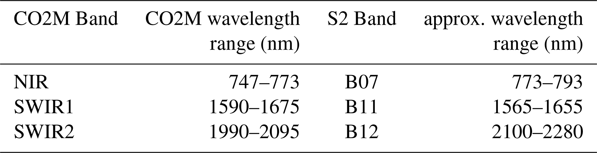
Although the spectral bands of the MSI do not exactly match with the bands measured by CO2M, they overlap sufficiently well to estimate the surface reflectance in the individual bands measured by CO2M. We use the bands B07 for NIR, B11 for SWIR1 and B12 for SWIR2, see Table 1, which have a surface reflectance precision in the order of 0.03 (Louis et al., 2019). Note that the time and viewing geometry are different between S2 and CO2M which is not relevant for the simulated data here, but could lead to errors in later applications, e.g. due to different shadows of the mountains at the time of measurement, if rain darkens part of the surface in the time between the two measurements, or if snow falls or melts in the meantime.

3.3 The FOCAL greenhouse gas retrieval algorithm

In this study, we use the Fast atmOspheric traCe gAs retrievaL (FOCAL) algorithm which approximates multiple scattering by one retrieved scattering layer (Reuter et al., 2017b). This makes FOCAL fast and efficient in retrieving trace gas information from hyperspectral instruments. FOCAL has been applied successfully to the measurements from many satellites like the Orbiting Carbon Observatory 2 (OCO-2, Reuter et al., 2017a), and the two Greenhouse gases Observing SATellites (GOSAT and GOSAT-2, Noël et al., 2021, 2022) and is one of the operational algorithms for the future CO2M mission which is used in this study (FOCAL-CO2M, Noël et al., 2024; Weimer et al., 2025).

The forward model of FOCAL-CO2M is used to generate a data base of simulated spectra which are used as a look-up table for the subpixel altitudes. Then, the subpixel radiances are averaged, similar to Eq. (1), resulting in the radiance for the spatial sample of the satellite, whereof XCO₂ is retrieved with FOCAL-CO2M using either the unweighted or the albedo-weighted surface altitude.

Table 2 State vector elements for FOCAL in this study with their a-priori values and usage in the fit windows.

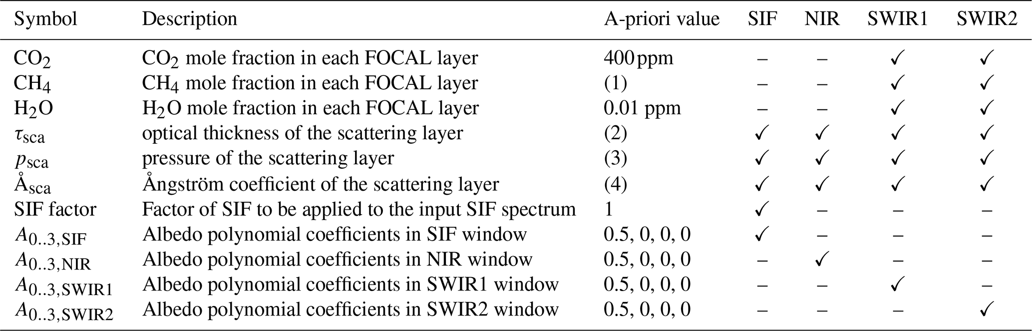
(1): Profile using the Simple cLImatological Model for atmospheric CH₄ (SLIMCH4, Noël et al., 2022) for the same grid cell over Berlin as the meteorological profiles. (2)–(4): depend on the scattering applied, see Appendix A: (2) 0.000, 0.019, 0.037; (3) 0.2000, 0.2635, 0.4880 in units of surface pressure; (4) 4.000, 3.575, 3.690.

The FOCAL forward model in this study generates spectra from the state vector elements listed in Table 2. They comprise the mole fractions of CO₂, CH₄ and H₂O, resolved in five layers with equal dry-air column, the properties of the scattering layer, a factor for the SIF signal and albedo polynomials in the fit windows. Note that further state vector elements are accounted for when applying FOCAL to real data, such as the shift and squeeze of the wavelengths (Reuter et al., 2017b).

The vertical meteorological profiles of pressure, temperature, dry-air column and geometric height are additional input for the forward model. For all cases analyzed in this study, the latter are taken from the ERA5 reanalysis (Hersbach et al., 2020) at a grid point over the capital of Germany, Berlin (latitude 52.51° N, longitude 13.4° E, surface elevation approx. 50 m) from 3 July 2015. The solar zenith angle is set to 50° in all cases. This ensures usage of realistic atmospheric conditions while keeping the basis of the meteorology constant to be able to study only the effect of surface altitude. In addition, consistency with the radiance database, described in the following section, is ensured with this so that the retrieved values are exactly the same for homogeneous scenes (not shown). The profiles are cut or extended to the actual DEM surface altitudes using the hydrostatic approximation. Then, they are resampled to the five FOCAL internal layers with equal dry-air sub-columns (see Reuter et al., 2017a). In the original version, they are the same for all wavelength bands, but here we are including a wavelength dependence, as discussed above. Therefore, we adapted FOCAL for this study to be able to use these meteorological profiles dependent on the wavelength bands, such that these variables get another dimension for the wavelength band and only the profiles for the specific wavelength band are used for fitting within this band. While using the same meteorological profiles from Berlin everywhere, they are cut off at or extended to the effective altitude for the specific fit window so that the profiles are different in each wavelength band. We provide these profiles either using the average surface altitude for all bands, or using the albedo-weighted altitude so that the profiles are different in the wavelength bands.

FOCAL-CO2M estimates the surface reflectance for each wavelength band (NIR, SWIR1, SWIR2) separately with a polynomial to account for non-linear effects, which are abbreviated as albedo polynomial coefficients in this study. As indicated in Sect. 2, the surface reflectance is wavelength-dependent, which makes the albedo-weighted averaged surface altitude dependent on the wavelength as well. Although, in principle, every single spectral measurement has a specific albedo, current satellite datasets, such as S2, provide information only for broader bands that are close to the fit windows used in FOCAL-CO2M.

The FOCAL algorithm uses optimal estimation to retrieve the state vector elements. All the state vector elements are set to the a-priori values of Table 2 and then iteratively calculated using the optimal estimation algorithm to retrieve XCO₂ and XCH₄, see e.g. Noël et al. (2024), and references therein. As can be seen, there is no direct connection of the NIR window to the XCO₂ concentration, only an indirect connection via the scattering parameters. We do not add noise to the radiances (but use a realistic uncertainty based on the signal-to-noise ratio). Then, we use the inversion of FOCAL to retrieve the state vector elements, one focus being XCO₂. We do not apply any post-processing but compare the directly retrieved XCO₂ between simulations with average and albedo-weighted averaged surface altitude. The experiments use average scattering parameters from the retrieval results by Weimer et al. (2025), see some further discussion of scattering in Appendix A

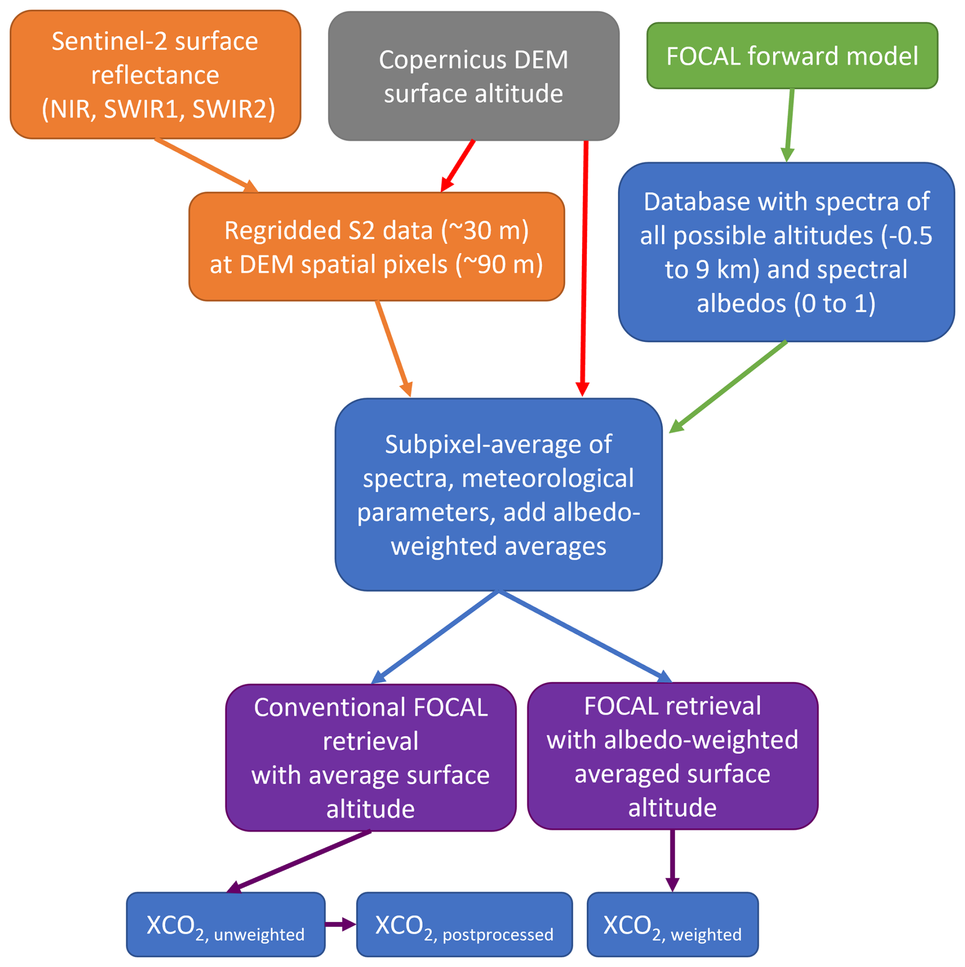
Figure 2 Flow chart illustrating the procedure starting from Copernicus DEM and S2 surface reflectance datasets to the XCO₂ retrievals with FOCAL.

3.4 Method to derive albedo-weighted average of surface altitude

In order to acquire the subpixel information about wavelength-dependent surface reflectance and surface altitude, the following procedure is applied (see Fig. 2):

First, we define the region of interest by using an S2 tile provided by the HLS dataset, average the S2 timeseries of cloud-free surface reflectance measurements using the data of the year 2019 for the 30 m pixels and additionally average the surface reflectances that fall into the Copernicus DEM spatial grid points with a side length of about 90 m. The year 2019 is used because it is the first full year of measurements of S2 with two satellites (better coverage) closest to the acquisition times in the CopDEM data. This results in surface reflectance measurements by S2 MSI at the same spatial sampling as the Copernicus DEM.

Secondly, we use the FOCAL forward model to generate a database of simulated radiance spectra for surface altitudes between −0.5 and 9 km with a vertical spacing of 4 m (i.e. CopDEM accuracy) and input surface reflectances for the three CO2M wavelength bands for values of $\mathit{\{}\mathrm{0.001},\mathrm{0.01},\mathrm{0.02},\mathrm{\dots },\mathrm{1.00}\mathit{\}}$. The input state vector elements for the FOCAL forward model are set to the a-priori values shown in Table 2. The input XCO₂ is set to a constant value of 400 parts per million (ppm), i.e. the CO₂ volume mixing ratio is set to this value in all internal FOCAL layers. The meteorological input parameters originate from the location of Berlin as mentioned above. Using the FOCAL forward model to generate the radiances has the advantage of self-consistency, i.e. in the homogeneous case, the radiance and therefore the retrieved XCO₂ will match exactly with the input. In other words, any deviation of the retrieved XCO₂ from 400 ppm is a direct result of errors in the surface altitude used in the retrieval. Therefore, it is representative to investigate the influence of this effect, although the effect of complex terrains is not explicitly accounted for as done in 3-dimensional radiative transfer algorithms (e.g., Shepherd and Dymond, 2003).

Thirdly, we take the CopDEM pixels that lie within one CO2M spatial sample and use the corresponding altitude and S2 reflectance data to obtain the simulated radiance measurement for each subpixel of the CO2M spatial sample. The number of subpixels n is on the order of 480 and is large enough to neglect that at the boundaries only parts of the CopDEM grid point are within the CO2M spatial sample. We then average the radiances across the CO2M spatial sample and interpolate the meteorological profiles to their corresponding average albedo and the average or albedo-weighted altitudes using a bilinear interpolation in the albedo-altitude space of the database of spectra.

Finally, we apply the FOCAL retrieval to the averaged spectra using both versions of the surface altitudes and compare their results for differences in the retrieved parameters, especially XCO₂. As the albedo is currently not measured simultaneously with the CO₂ measurements, we also explore the option to apply a post-processing to already retrieved XCO₂, which is indicated with the subscript “postpro” in this study (see Sect. 4.4 for further information).

4 Results

We start by applying this methodology to idealized conditions (Sect. 4.1) where we define the subpixel surface altitudes and albedos. The complexity of these experiment is increased incrementally to test whether the one-wavelength model of Sect. 2 is applicable to the actual multi-wavelength retrieval algorithm. Then, we apply the methodology to realistic scenes on Earth as examples, see Sect. 4.2. This is followed by examination of the question of whether the surface roughness thresholds in greenhouse gas retrievals can be relaxed when using the albedo-weighted average of the surface altitude in Sect. 4.3. Then, the possible application in greenhouse gas retrievals as post-processing (Sect.  4.4) and in comparison to the direct implementation in FOCAL is investigated (Sect. 4.5). Finally, we examine the dependence of the effect on different sizes of satellite spatial samples in Sect. 4.6.

4.1 Application to idealized conditions

In a first experiment, we separate an artificial satellite spatial sample into two parts, similar to the simple example of Fig. 1, but the fraction f of the dark and bright parts may vary between 0 and 100 %. One part of the spatial sample has a surface altitude of 0 m and albedo values in all wavelength bands of 0.001. The value 0.001 is used because a value of zero is unrealistic and leads to errors in the retrieval. The values in the other parts vary as described below. In the one-wavelength example of Eq. (1), this can be calculated explicitly. We are now interested in the difference of c, if we use the average altitude instead of the albedo-averaged altitude, while the measured radiance is the same:

$$\begin{array}{}\text{(24)}& {\displaystyle }{I}_{\mathrm{weighted}}=I_{\mathrm{0}}\mathit{\alpha }\exp \left[-d_{\mathrm{0}}\mathit{\sigma }{c}_{\mathrm{weighted}}\exp \left(-{\displaystyle \frac{z_{\mathrm{s},\mathrm{weighted}}}{H}}\right)\right]\text{(25)}& {\displaystyle }{I}_{\mathrm{mean}}=I_{\mathrm{0}}\mathit{\alpha }\exp \left[-d_{\mathrm{0}}\mathit{\sigma }{c}_{\mathrm{mean}}\exp \left(-{\displaystyle \frac{z_{\mathrm{s},\mathrm{mean}}}{H}}\right)\right]\text{(26)}& {\displaystyle }{I}_{\mathrm{weighted}}\stackrel{!}{=}{I}_{\mathrm{mean}}.\end{array}$$

The difference in XCO₂ can then be written as:

$$\begin{array}{}\text{(27)}& \begin{array}{rl}\mathrm{\Delta }c& =c_{\mathrm{weighted}}-c_{\mathrm{mean}}\\ & =c_{\mathrm{weighted}}\left[\mathrm{1}-\exp \left({\displaystyle \frac{z_{\mathrm{s},\mathrm{mean}}-z_{\mathrm{s},\mathrm{weighted}}}{H}}\right)\right]\end{array}\end{array}$$

with z_s,weighted and z_s,mean depending on the fraction f filled with α₂ as:

$$\begin{array}{}\text{(28)}& {\displaystyle }{z}_{\mathrm{s},\mathrm{weighted}}={\displaystyle \frac{(\mathrm{1}-f){\mathit{\alpha }}_{\mathrm{1}}{z}_{\mathrm{s},\mathrm{1}}+f{\mathit{\alpha }}_{\mathrm{2}}{z}_{\mathrm{s},\mathrm{2}}}{(\mathrm{1}-f){\mathit{\alpha }}_{\mathrm{1}}+f{\mathit{\alpha }}_{\mathrm{2}}}}\text{(29)}& {\displaystyle }{z}_{\mathrm{s},\mathrm{mean}}=(\mathrm{1}-f)z_{\mathrm{s},\mathrm{1}}+f{z}_{\mathrm{s},\mathrm{2}}.\end{array}$$

Note that we define ΔXCO₂ as a correction term to the retrieved XCO₂ throughout this study. Thus, the resulting ΔXCO₂ has to be added to the retrieved XCO₂ to get the XCO₂ corrected for the effect of albedo-weighted averaged surface altitude.

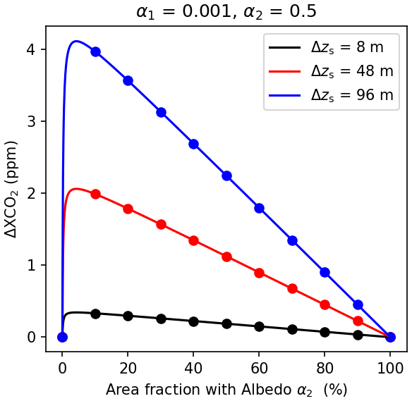
Figure 3 Differences of XCO₂ between averaged and albedo-weighted average of the surface altitude for a spatial sample split into two parts for fractions filled with albedo α₂ between 0 and 100 %, albedo values of the parts of α₁=0.001 and α₂=0.5. The simple one-wavelength model is used, resulting in Eq. (27), which is shown here. The three lines correspond to altitude changes with respect to the average surface altitude (Δz_s) of 8, 48 and 96 m. We added dots at the fractions that are used in the next two figures of this study for comparison. More examples of albedo pairs can be found in the Supplement this study (Fig. S1).

An example of this equation for α₁=0.001 and α₂=0.5 is shown in Fig. 3 for different subpixel surface altitude changes (8, 48 and 96 m, where 96 m corresponds to the maximum subpixel altitude changes of the Black Forest in Germany if CO2M-sized spatial samples are assumed to be split in two parts). Due to the non-linearity in f, the difference in XCO₂ depends on the fraction in a strongly non-linear and asymmetric way. We show some more examples of albedo pairs in the Supplement where it can be seen that this asymmetry is due to the small value of α₁=0.001. As expected, ΔXCO₂ increases with an increasing Δz_s, with values up to ΔXCO₂≈4 ppm for Δz_s=96 m.

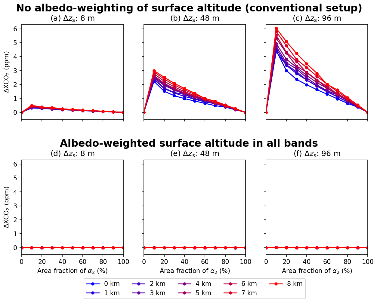
Figure 4 Dependence of ΔXCO₂ in a spatial sample split into two homogeneous parts retrieved with FOCAL on background altitude (line colors), altitude difference Δz_s (columns) and using the unweighted (top row) and albedo-weighted average (bottom row) of the surface altitude. The x-axis shows the fraction f (different lines) of the artificial satellite spatial sample, split into two parts. The albedos of the three wavelength bands of CO2M are set to α₁=0.001 and α₂=0.5, as in Fig. 3. Because some of the panels have values that are close to zero, we added the figures without shared y-axes in the Supplement of this study (Fig. S2).

We further extend this experiment and apply the FOCAL retrieval algorithm to this spatial sample with all wavelength bands and fit windows as in CO2M for the same albedo values in all three bands, see Fig. 4. This figure gives a first indication that the albedo-weighted average of the surface altitude should be used in nadir satellite retrievals because the differences in XCO₂ are by two orders of magnitude smaller using this approach compared to the average altitude. As expected from the theoretical example of Fig. 3, the largest differences occur for a fraction of 10 % and the order of magnitude of the changes is similar. The non-monotonous values within one fraction are a result of the retrievals that are not equal to the truth anymore so that other retrieved parameters get involved in the calculation.

Figure 4 also shows the dependence of ΔXCO₂ on the background surface altitude which varied between zero and 8000 m. The deviation of ΔXCO₂ from zero increases in all cases with increased background altitude. This cannot directly be explained by the simple theoretical model above, and has probably to do with using more than one wavelength for the cross sections and more than one trace gas to be retrieved which leads to larger complexity.

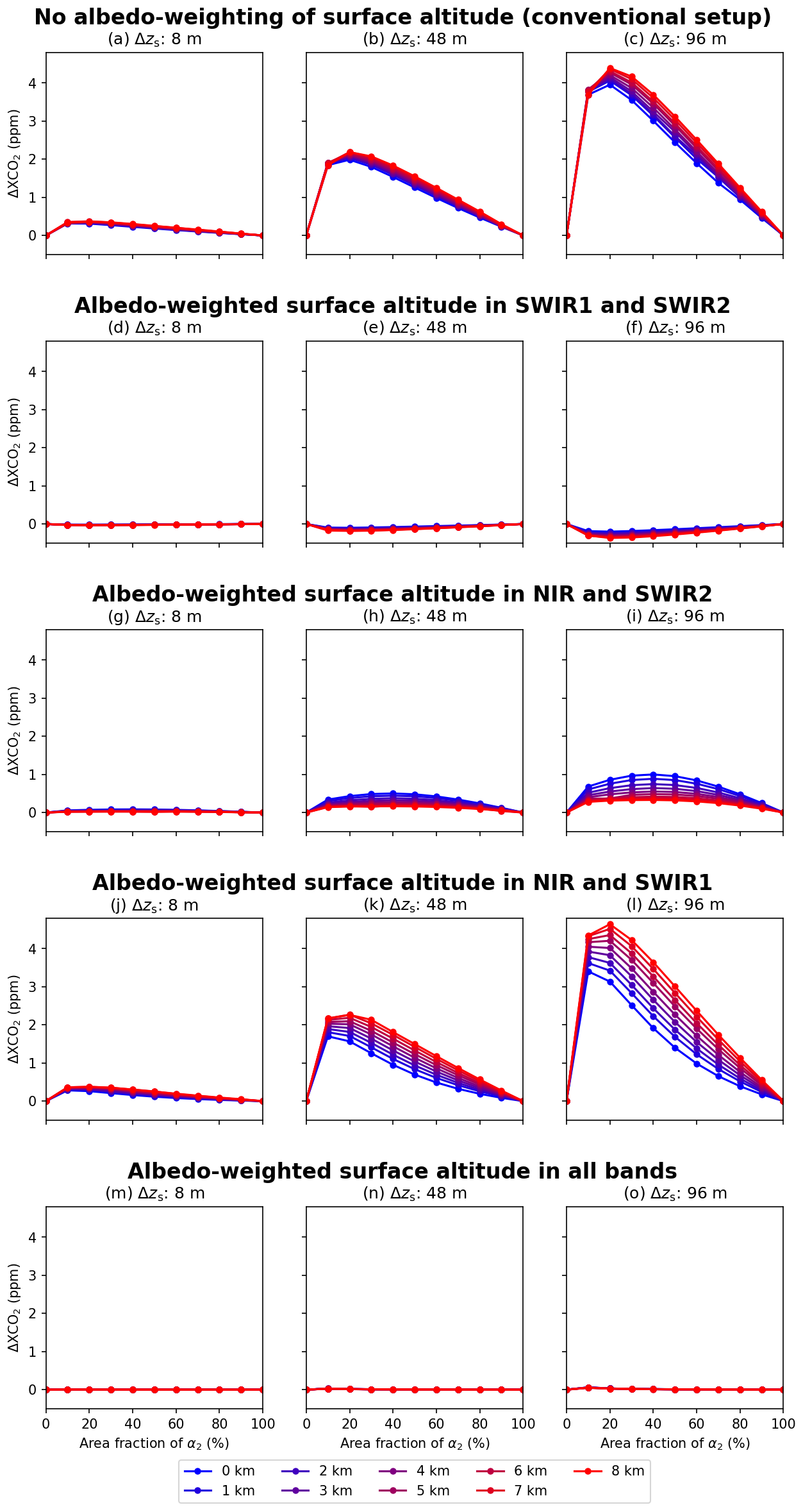
Figure 5 Similar to Fig. 4, but showing results with the VEG50 scenario in the second part of the spatial sample split into two, i.e. ${\mathit{\alpha }}_{\mathrm{NIR},\mathrm{2}}=\mathrm{0.2}$, ${\mathit{\alpha }}_{\mathrm{SWIR}\mathrm{1},\mathrm{2}}=\mathrm{0.1}$, ${\mathit{\alpha }}_{\mathrm{SWIR}\mathrm{2},\mathrm{2}}=\mathrm{0.05}$ (ESA, 2020). Additional experiments where the average surface altitude is taken in only one of the three bands are shown (second to fourth row). In the other bands, the albedo-weighted average of the surface altitude is used. As in some of the panels the values are close to zero, we added the figures without shared y-axes in the Supplement of this study (Fig. S3).

The previous examples showed cases where the albedo is the same in the three wavelength bands. As a next step, we set the albedos to the values of the VEG50 scenario described in ESA (2020), see Fig. 5. In general, ΔXCO₂ is smaller than with albedo 0.5 and the height dependence is smaller as well. Similar to the previous analysis, ΔXCO₂ is small for the case of an albedo-weighted average of the surface altitude with values of about ±0.15 ppm. In addition to the experiments shown in Fig. 4, we show experiments in Fig. 5 where the average surface altitude is used in the retrieval only in one wavelength band so that contributions of the different bands to the XCO₂ error can be estimated. As expected, the contributions of the SWIR bands are largest due to their sensitivity to the CO₂ concentration in the atmosphere. The largest contributions originate from the SWIR2 band. The ΔXCO₂ values due to the NIR band are smaller but not negligible for the VEG50 scenario. The largest XCO₂ changes occur for a fraction of the spatial sample of f=20 % as a result of the different albedo values compared to the previous analysis. Note that the ΔXCO₂ values due to the SWIR1 band (third row in Fig. 5) show the expected decrease with the background altitude so that it can be concluded that the increase seen in the unweighted average comes from the SWIR2 band. In addition, it can be seen that the error at 8 km is larger when applying the average only in the SWIR2 band compared to the average in all bands, which shows that the error in the first row is a linear combination of the error in all bands. As the SWIR2 band has the largest contribution, the order of the lines in the first row of Fig. 5 is similar to the experiment with average surface altitude only in the SWIR2 band.

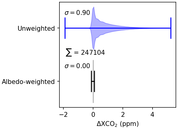
Figure 6 Differences of XCO₂ for all combinations of a spatial sample split into two parts, with one part $z_{\mathrm{s},\mathrm{1}}=\mathrm{0}\mathrm{m}$ and albedo of 0.001 in all fit windows, and the other part changing z_s,2 between $\left\{\mathrm{0},\mathrm{8},\mathrm{\dots },\mathrm{96}\mathrm{m}\right\}$, spectral band albedos between $\left\{\mathrm{0.001},\mathrm{0.05},\mathrm{0.1},\mathrm{0.2},\mathrm{\dots },\mathrm{1}\right\}$ and fractions between $\left\{\mathrm{0},\mathrm{0.1},\mathrm{\dots },\mathrm{1}\right\}$. The blue graph corresponds to the experiment with mean surface altitude and the black graph shows the experiment with albedo-weighted averaged surface altitude. The horizontal lines show minimum and maximum and the shaded ranges show the distribution of values. The total number of data points is 247 104 (12³ albedo, 13 altitude and 11 fraction values). The σ values correspond to the standard deviations of the XCO₂ values (in ppm).

We extended the analysis to not only one combination of albedos and z_s,2 values, but performed experiments with all combinations of Δz_s, α_NIR,2, α_SWIR1,2, α_SWIR2,2 and fractions f and compared the results of ΔXCO₂ between retrievals using mean and albedo-weighted surface altitude, see Fig. 6. While the experiment using the average surface altitude shows differences of up to 5 ppm, the variability of ΔXCO₂ in the experiment with albedo-weighted surface altitude is much smaller. This is also reflected in the standard deviations for both methods: With the unweighted average, the standard deviation is 0.9 ppm whereas it is 0.01 ppm when applying the albedo-weighted average of the surface altitude. The negative differences in Fig. 6 are a result of near-zero albedo values in the SWIR bands and a non-zero albedo in the NIR. There is some dependence on Δz_s for the experiment with albedo-weighted surface altitude which is a result of the approximations discussed in Sect. 2.

In summary, it was shown in this section starting from a theoretical example with constant conditions and ending with variable surface altitudes, albedos and fractions that the albedo-weighted averaged surface altitude is a good approximation for the surface altitude that is representative for the light path in a spatial sample of a satellite. As the experiments shown above always used an artificial spatial sample split into two homogeneous parts, these test cases are useful to investigate the results in defined conditions. In reality, the structure of Earth's surface is more complex, therefore we apply our method to real albedo values and orography and real numbers of subpixels in the next section.

4.2 Application to real topography

The methodology described in Sect. 3.4 is now applied to real scenes, and the examples shown in this section comprise the Bełchatów power plant in Poland with an open pit coal mining area next to the power plant (Sect. 4.2.1), the Black Forest, a mountain range in Germany (Sect. 4.2.2), a region around the Mont Blanc, the highest mountain in the European Alps (Sect. 4.2.3) and the whole country of Germany (Sect. 4.2.4). We first select the tiles in the HLS dataset that include these locations, given in Military Grid Reference System coordinates, and a CO2M orbit (simulated by EUMETSAT, also input for Noël et al. (2024) and Weimer et al. (2025)) that covers the whole region. Then we select the CopDEM grid points that are in this area and apply the method as described in Sect. 3.4.

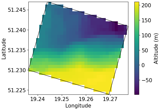
Figure 7 Example of the CopDEM surface altitude values within a spatial sample (black line) of CO2M at the edge of the Bełchatów open pit coal mining area.

4.2.1 The Bełchatów Power Plant

The Bełchatów power plant in Poland is one of the strongest point sources of CO₂ emissions in Europe and has been a test case for many remote sensing applications (e.g., Cusworth et al., 2021; Nassar et al., 2022; Brunner et al., 2023; Fuentes Andrade et al., 2024; Jacobs et al., 2024; Moeini et al., 2025). The surrounding surface structure is challenging because of the open pit coal mining area next to the power plant (Jacobs et al., 2024), and because trace gas retrievals depend on a precise knowledge of the surface altitude. In addition, the surface altitude around open pit coal mining areas changes over time at this location due to the anthropogenic interference. Figure 7 shows an example of a spatial sample of CO2M at the edge of the Bełchatów coal mining area. Large subpixel altitude changes of more than 250 m within one spatial sample occur.

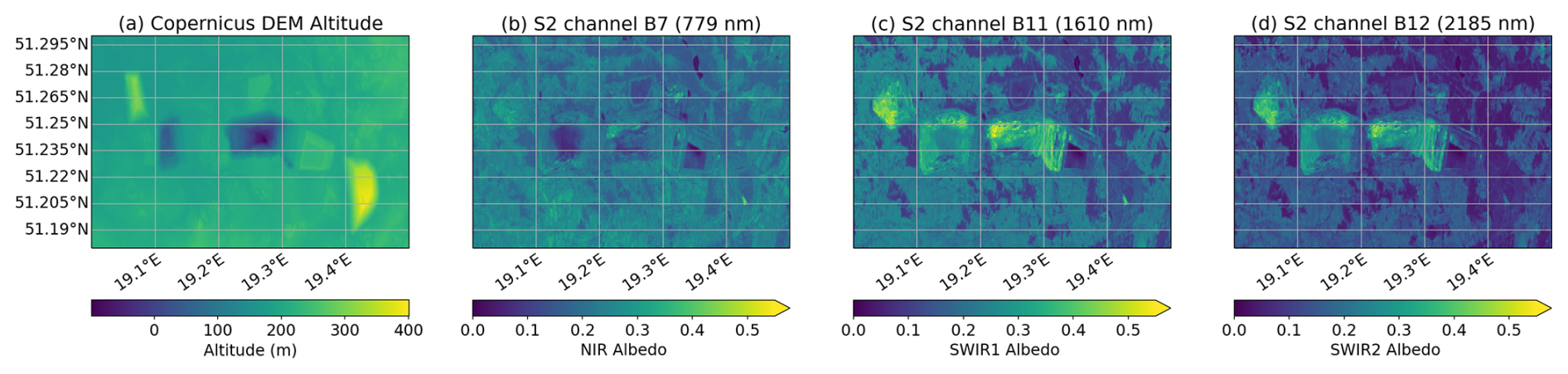
Figure 8 (a) Surface altitude by CopDEM and surface reflectance by S2 regridded to CopDEM grid points in the (b) NIR, (c) SWIR1 and (d) SWIR2 at the Bełchatów coal mining area.

In addition to significant changes in the surface altitude, the anthropogenic activities in the coal mining field reveal areas that have low albedo in the NIR, but larger albedo in the SWIR bands compared to the surrounding. Figure 8 shows the surface altitude and albedo values where it can be seen that the coal mining field is brighter in the SWIR bands but darker than the surrounding in the NIR band. Therefore, the albedo-weighted altitude, which has been shown to better represent the effective altitude of the column in the previous section, will be smaller in the SWIR bands than in the NIR band.

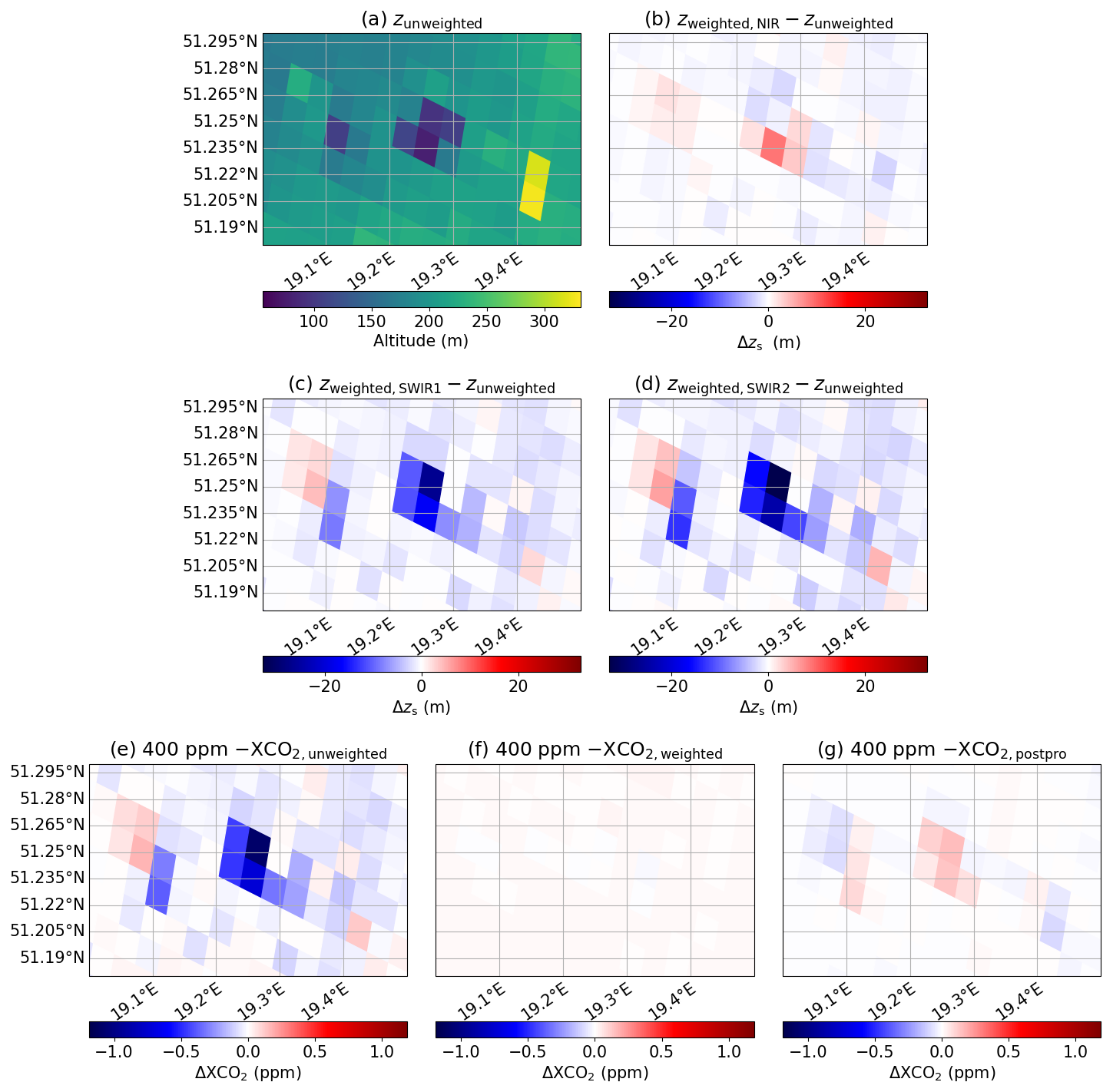
Figure 9 (a) Average surface altitude and (b)–(d) the deviation of the albedo-weighted average for the Bełchatów power plant at simulated CO2M spatial samples. The deviations from the true value of XCO₂=400 ppm are shown in the bottom row for (e) the unweighted, (f) the albedo-weighted surface altitude and (g) after applying the post-processing equation to XCO_2,unweighted, see Sect. 4.4.

As a result, differences of more than 25 m in the effective altitude occur at the location of the coal mining field for CO2M-sized spatial samples, see Fig. 9b–d. Furthermore, the different albedo values in the wavelength bands result in different signs of the altitude anomaly in the NIR and SWIR bands. The actual altitude to be used in the NIR band is up to 8 m larger and in the SWIR2 band up to 32 m smaller than the average surface altitude. The altitude differences in the SWIR1 band are correlated with the SWIR2 differences, but smaller in magnitude.

These deviations in the surface altitude have an impact on the retrieved XCO₂, see Fig. 9e–g. As described above, the input XCO₂ for all retrievals is 400 ppm and any difference from this value can be attributed to the effect of surface altitude. Hence, there is a correlation between the altitude changes in the SWIR bands and the XCO₂ changes using the average surface altitude (panel e), which will be further analyzed in Sect. 4.4. In addition, Fig. 9f shows the ΔXCO₂ using the albedo-weighted surface altitudes. As can be seen, changes of XCO₂ on the order of 1 ppm occur when using the average surface altitude. When applying the albedo-weighted averaged surface altitude, the structure of the coal mining field vanishes and the variation of XCO₂ is one order of magnitude smaller. Therefore, this figure shows that the albedo-weighted averaged surface altitude is a better approximation of the surface altitude representative of the satellite measurement also for real orographies and albedo values, and that this approach should be used in trace gas retrievals.

The Bełchatów power plant is an example where anthropogenic interference leads to local and continued differences of surface altitude and surface albedo, which then can also impact emission estimates of the nearby power plant. We will show in the next sections that the effect of altitude-albedo changes also affects inhomogeneous scenes that are dominated by natural environments.

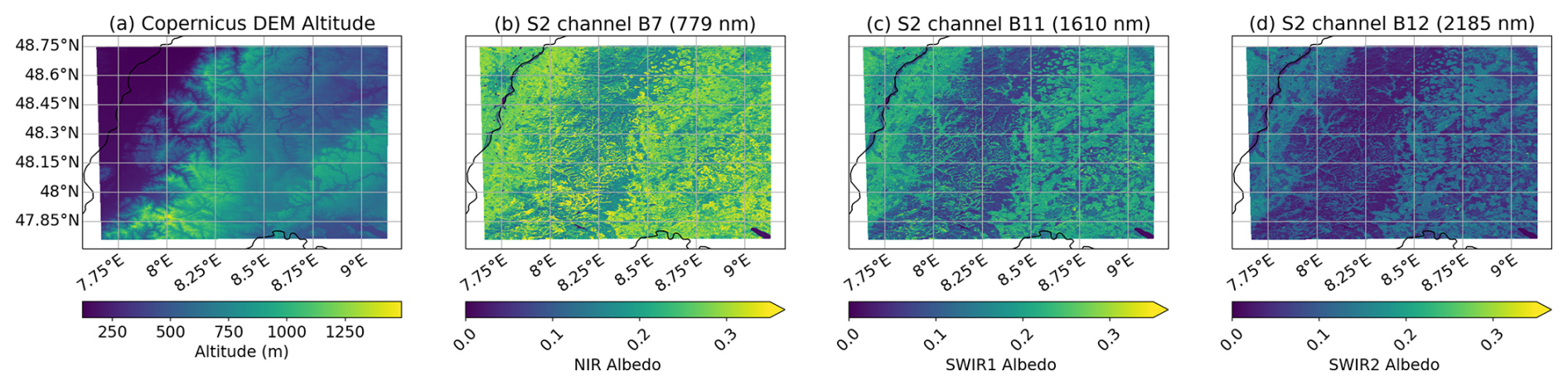
Figure 10 (a) Surface altitude by CopDEM and surface reflectance by S2 regridded to CopDEM grid points in the (b) NIR, (c) SWIR1 and (d) SWIR2 in the Black Forest.

4.2.2 Black Forest

The Black Forest is a mountain range located in Southwest Germany with mountains reaching altitudes up to about 1500 m above sea level, see panel (a) of Fig. 10. The different vegetation results in changes of the surface albedo combined with surface altitude changes and is representative for mountain ranges in Germany and the mid-latitudes. Agricultural activity and small towns lead to generally higher albedo values in the valleys of the Black Forest compared to the forest regions at higher altitudes. Water bodies, such as rivers and lakes, have low albedo values in all wavelength bands. In total, the albedo values in panels (b) to (d) show some surface structure, but the differences in albedo are smaller than in the Bełchatów example above. Nevertheless, there are differences in the albedo of the SWIR bands (panels c and d) compared to the NIR band (panel b) arising from the differing wavelength dependence of the different surface types.

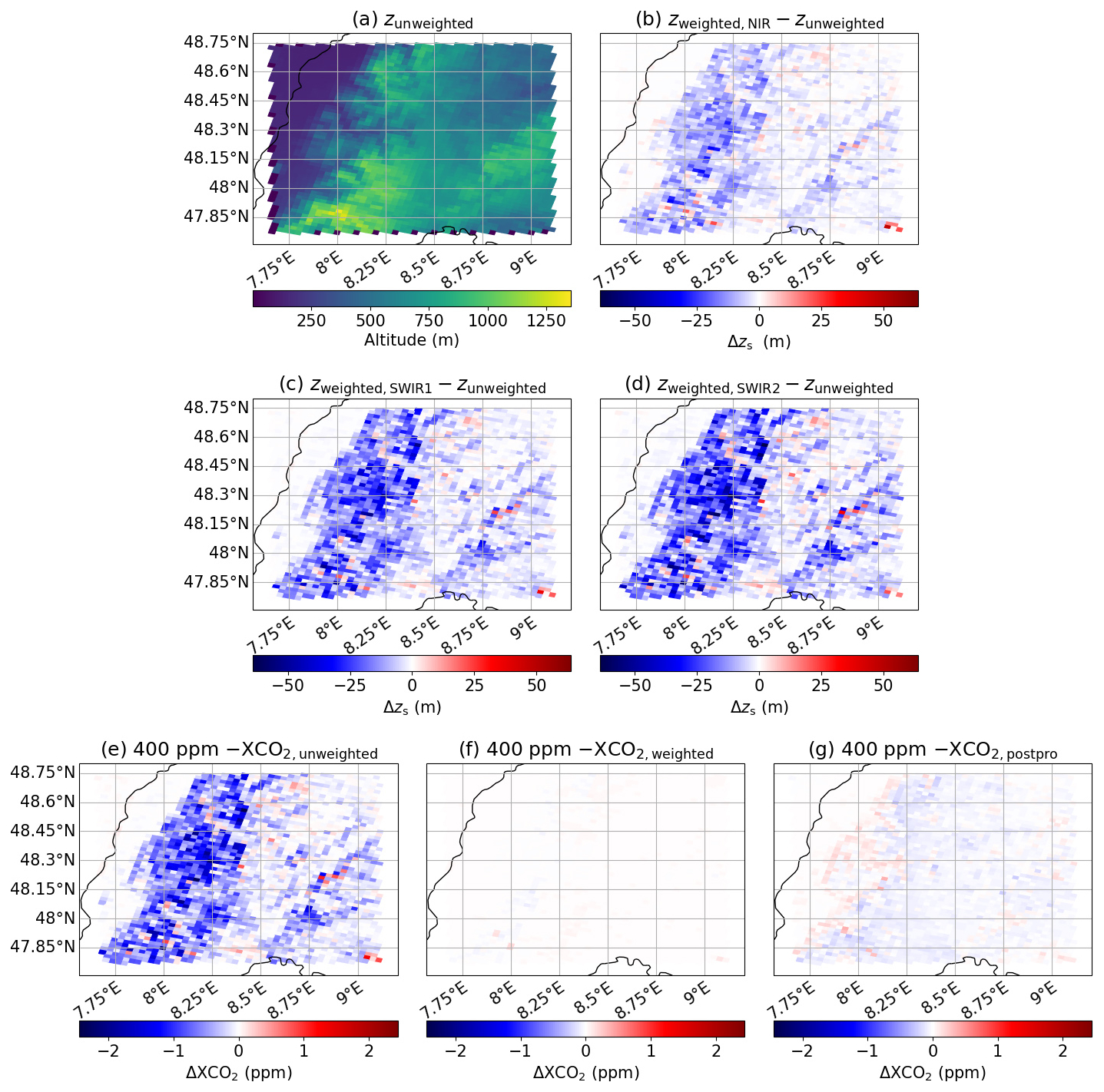
Figure 11 Same as Fig. 9, but for the Black Forest region.

Due to the variation in altitude and albedo, differences of up to 60 m occur over the Black Forest when using the albedo-weighted average, see Fig. 11b–d. Differences are smaller in the NIR band than in the SWIR bands, which are more sensitive to the surface types, e.g. whether the surface is rocky or covered by trees. The changes in the SWIR bands are correlated although the local magnitude differs depending on the subpixel surface variability.

Panels (e) to (g) of Fig. 11 show the impact on XCO₂ for the Black Forest region. Values of ΔXCO₂ larger than 2 ppm occur over the Black Forest when using the average surface altitude, which is more than four times larger than the requirement for systematic differences of 0.5 ppm for CO2M (ESA, 2020). Note that this bias could be confused with CO₂ respiration by the biosphere, showing the need to account for this process in greenhouse gas retrievals.

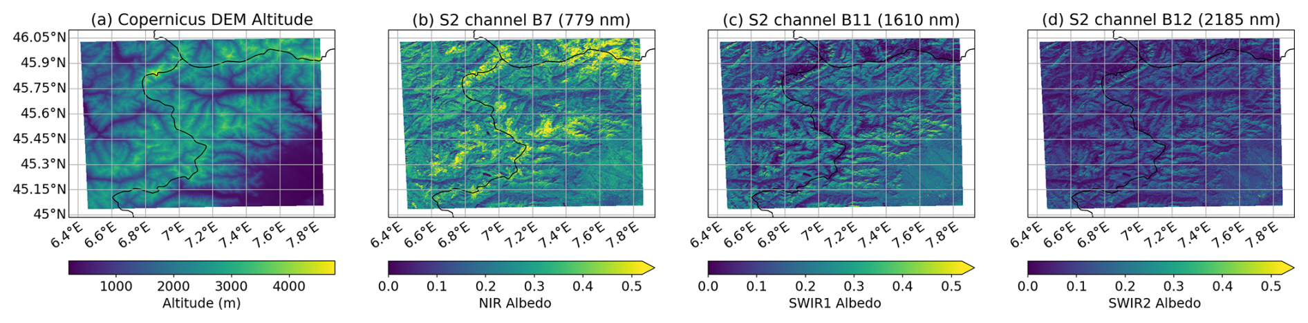
Figure 12 (a) Surface altitude by CopDEM and surface reflectance by S2 regridded to CopDEM grid points in the (b) NIR, (c) SWIR1 and (d) SWIR2 at region around Mont Blanc.

Due to the increased surface roughness in these regions, these spatial samples used to be filtered out during the retrieval process. However, when using the albedo-weighted average of the surface altitude, these differences are decreased to values smaller than 0.2 ppm, showing the potential of this method for increasing the coverage over regions with larger surface roughness.

4.2.3 Mont Blanc

Mountain regions such as the Alps are usually filtered due to large surface roughness, shadow effects, slopes of the mountains and generally the heterogeneity of the surface properties. In addition, it was estimated that larger surface roughness will lead to larger errors when applying the first-order approximation using Eq. (23). Therefore, we expect high mountain regions, such as around the Mont Blanc, the highest mountain of the European Alps, to show remaining biases even after applying the albedo-weighted average of the surface altitude. This region is chosen to assess how large this effect is when pushing the methodology and the retrieval towards the edge of their applicability. Although these data probably have to be filtered, we investigate these regions, too, because biases in these regions may also be reduced by our method.

Figure 12 shows the surface altitude of the CopDEM and the albedo in the respective S2 bands for the region around Mont Blanc. The altitude varies between close to zero up to 4800 m, showing the challenging conditions for the retrieval. In valleys, the altitude can be lower than 1000 m whereas on top of the close-by mountains the altitude is usually approximately 3000 m.

In addition, the surface types change with altitude: At low altitudes, the surface is covered by trees and may be partly covered by water bodies like rivers or lakes. At higher altitudes, they are replaced by a rocky surface, which may be covered by snow. All of these conditions have an impact on the albedo in the NIR and SWIR. For instance, at the top of Mont Blanc (45.9° N, 7.0° E), snow leads to increased albedo in the NIR but to a decreased albedo in the SWIR bands. Rivers lead to low albedo in the valleys in all three bands. A rocky surface has higher albedo in the SWIR than in the NIR, so that, altogether, differences in the effective altitudes can be expected in the mountainous region of Fig. 12.

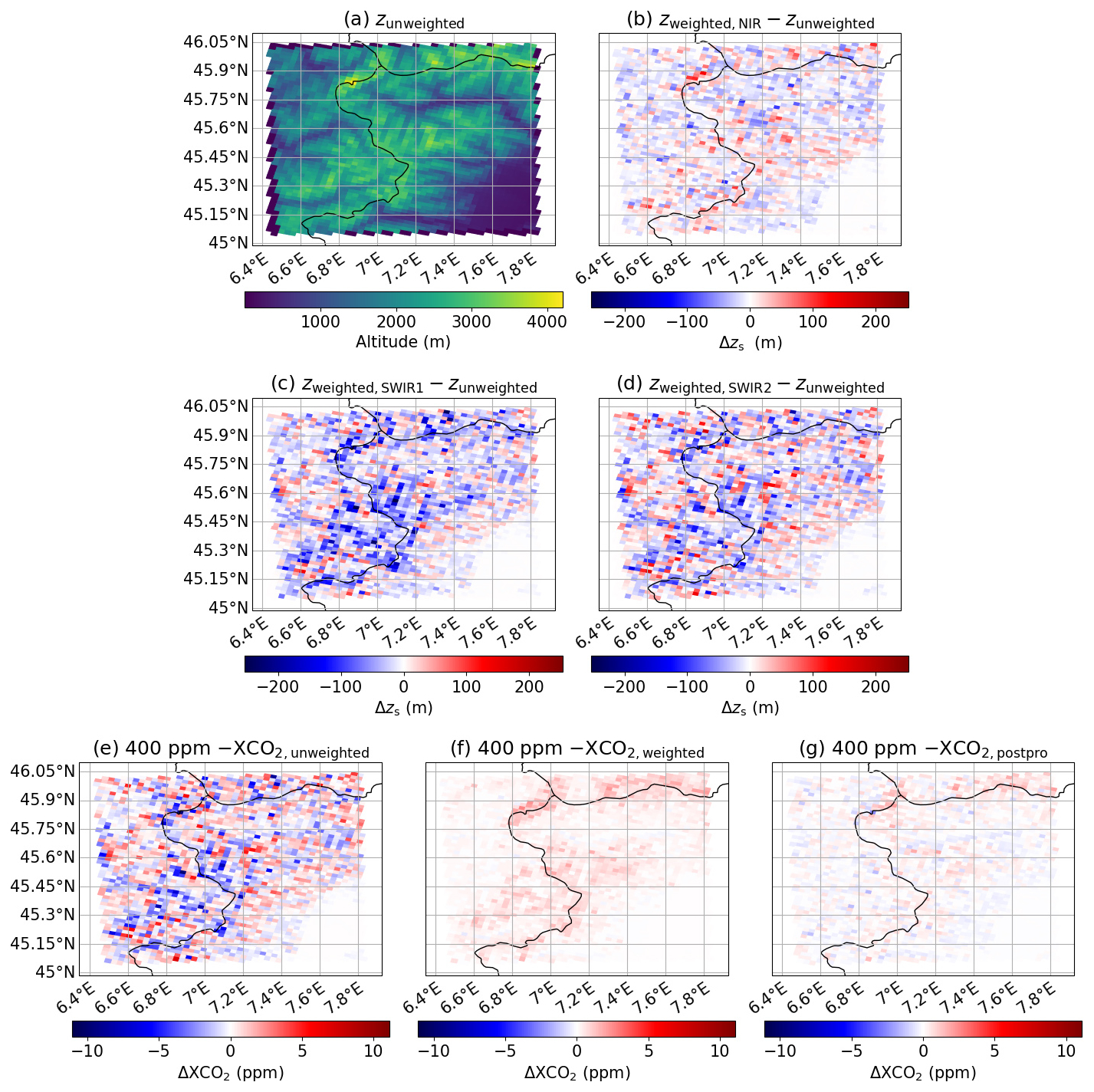
Figure 13 Same as Fig. 9, but for the region around the Mont Blanc.

The differences in the surface altitude for CO2M spatial samples are shown in Fig. 13b–d, together with the average surface altitude in panel (a). As expected, the differences are larger for the Mont Blanc region than for the Black Forest due to the larger subpixel altitude and albedo variability. Differences up to ±230 m occur in this region with the largest negative differences in the SWIR1 band and the largest positive changes in the SWIR2 band. In the NIR, the permanently snowy surface shows differences larger than zero whereas they are negative in the SWIR bands. As there are regions on the Earth where snow cover depends on the season, this also highlights the need for wavelength-dependent albedo data simultaneously measured with the greenhouse gas measurements.

These differences in the surface altitude lead to changes in XCO₂, which are shown in Fig. 13e–g for the Mont Blanc region. Due to the larger differences of the surface altitude locally on the order of 200 m, the differences in ΔXCO₂ are larger, locally down to −10 ppm. The differences in XCO₂ using the albedo-weighted average of the surface altitude are larger than for the previous examples with values up to ±2.5 ppm and showing patterns of the highest mountains in the scene. This is a result of the approximation using Eq. (23) which showed some dependence on the surface roughness. Nevertheless, the overall variability of ΔXCO₂ is still much smaller when using the albedo-weighted altitude compared to using the unweighted average of the surface altitude. On the other hand, it is clear that this estimated bias up to ±2.5 ppm is larger than the accuracy requirement for CO2M so that they will likely be filtered out in retrievals with real satellite data.

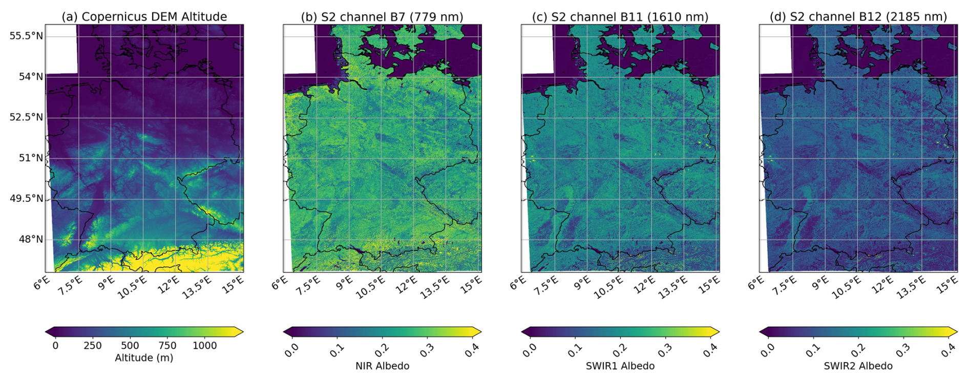
Figure 14 (a) Surface altitude by CopDEM and surface reflectance by S2 regridded to CopDEM grid points in the (b) NIR, (c) SWIR1 and (d) SWIR2 in Germany. We added a figure with the complete color scales to the Supplement of this study (Fig. S4).

4.2.4 Germany

As a final example, we show the results of the whole country of Germany. The surface altitude from CopDEM and the albedos in the three wavelength bands are shown in Fig. 14. Note that we focus on the lower altitudes in Germany here and therefore cut the color scales accordingly. Figures with the full color scales can be found in the Supplement of this study. The surface altitude variation is larger in Southern Germany than in the northern part with values in the mountain ranges up to about 1500 m. The average albedo is largest in the NIR and smallest in the SWIR2 range with local differences, as shown in the previous examples. The general patterns of the albedo are similar between SWIR1 and SWIR2. Some locations show large albedo values in the SWIR bands in the east of Germany close to the border to Poland (at about 51.5° N, 14.5° E), around 51° N, 12° E and in the west of Germany close to the border to the Netherlands around 51° N, 6.5° E. They are the open pit coal mining fields in Germany, which show an effect similar to that at Bełchatów in Sect. 4.2.1 but with smaller amplitude in the altitude changes.

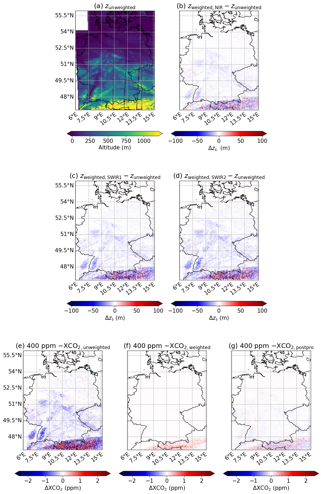
Figure 15 Same as Fig. 9, but for the whole country of Germany. We added a figure with the complete color scales to the Supplement of this study (Fig. S5).

The changes in surface altitude for Germany, shown in Fig. 15b–d, are smaller in the NIR than in the SWIR bands. Apart from the Alps region, the largest negative differences occur over the Black Forest. Some locations show positive altitude changes, such as a part of the Rhine river valley at around 50° N, 8° E, which is relatively narrow and which has lower albedo in the valley than on the surrounding slopes. A similar positive pattern is seen for some lakes in the north west and southern part of Germany.

Similar to the previous results of this section, these differences in altitude can be translated to changes in XCO₂, see Fig. 15e–g. ΔXCO_2,unweighted in panel (e) is correlated with the altitude changes in the SWIR bands, which will be further analyzed in Sect. 4.4. In contrast, ΔXCO₂ using the albedo-weighted averaged surface altitude (panel f) varies only between ±0.3 ppm.

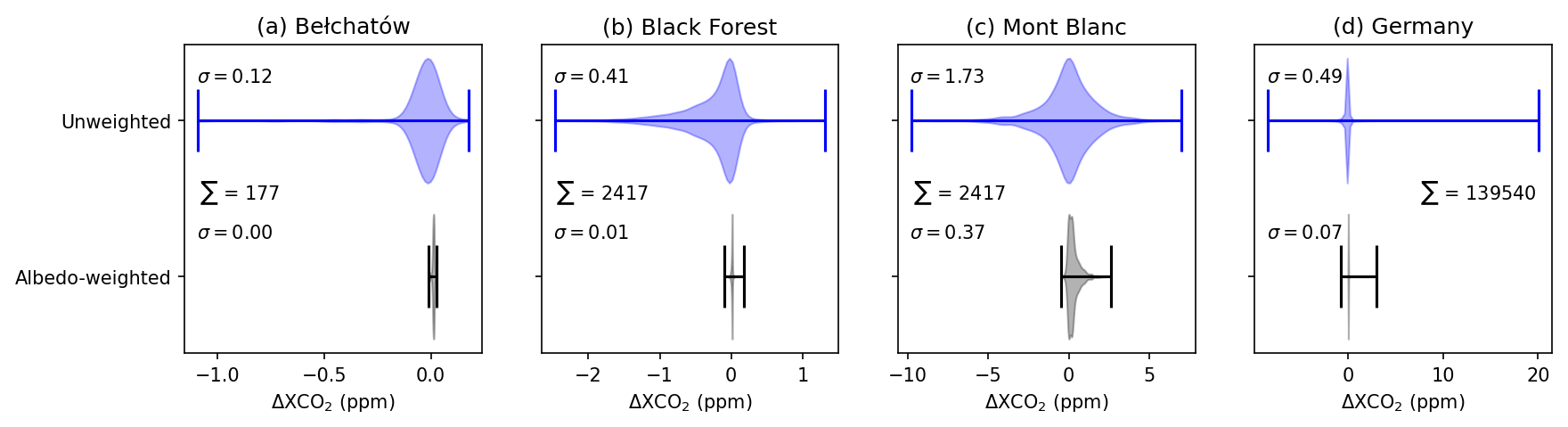
Figure 16 Variability of ΔXCO₂ for the regions discussed in this section: (a) Bełchatów, (b) Black Forest, (c) Mont Blanc and (d) Germany. Note that the total number of data points differs largely between the panels. The σ values correspond to the standard deviations of the XCO₂ values (in ppm).

4.2.5 Overall Variability of XCO₂

In order to summarize the results of this section, Fig. 16 shows the overall variability of XCO₂ for both approaches, using the unweighted average of the surface altitude, as is currently done in trace gas retrievals, and using the method suggested in this study with albedo-weighted averaged surface altitude as input to the retrieval. Similar to Fig. 6, each panel shows the distribution of the XCO₂ deviation from 400 ppm and the extreme values for all regions discussed in this section. Note that the number of data points is different for each region, as shown by the ∑ sign in the panels.

At the Bełchatów Power Plant (panel a), only a few CO2M spatial samples cover the coal mining field so that the distribution is similar for both methods, but the extreme values are largely reduced by using the albedo-weighted average for the surface altitude, which also reduces the standard deviation from 0.12 to 0.05 ppm. On the one hand, this demonstrates that the new method does not change the cases where the average altitude is already a good approximation. On the other hand, this demonstrates that the errors due to the average surface altitude are reduced using the albedo-weighted surface altitude.

The fraction of small altitude differences is smaller in the other regions so that the distributions are broader using the mean altitude than for the albedo-weighted altitude. In the case of the Black Forest (panel b), the distribution is skewed towards negative ΔXCO₂ values and the extreme values are reduced by a factor of 10. The standard deviations are reduced from 0.41 to 0.05 ppm. Due to the valley effect with vegetation at lower altitudes and in combination with rock and snow at the top of the mountain, the distribution in the region around the Mont Blanc (panel c) is symmetric around zero when using the mean altitude with extreme values of −10 and 7 ppm in ΔXCO₂. Also in this region, these extreme values are reduced and the distribution is narrower when using the albedo-weighted surface altitude, resulting in a reduction of the standard deviation from 1.78 to 0.39 ppm. Similar effects can be seen in the whole country of Germany (panel d), now including the Alps region in the south, which dominates the extreme values in this case. The extreme values are reduced and the overall distribution is narrower when using the albedo-weighted averaged surface altitude with a reduction of the standard deviation from 0.52 to 0.09 ppm.

Hence, we showed in this section that there might be a benefit in using the albedo-weighted average for the surface altitude in a variety of cases with real topography. As the albedo-weighted average of the surface altitude is still an approximation, remnants of the surface structure are visible using this approach, but the XCO₂ bias for heterogeneous surface structures is largely reduced.

4.3 Dependence of XCO₂ errors on the surface roughness

Surface roughness, defined as the standard deviation of the sub-pixel surface altitudes by the CopDEM altitude values here, is a possible filtering parameter during pre-processing of trace gas retrievals. Too large surface roughness usually means that the conditions are too challenging for the retrieval so that they might be excluded in advance from the computation. In this section, we investigate if using the albedo-weighted surface altitude can lead to a relaxation of these criteria. In order to get a range of surface roughness values as large as possible, we apply the methodology not only to the regions described above, but also to the whole region of the Alps, the Pyrenees, and some regions at the highest points of Scandinavia and the Andes, resulting in a total of about 30 million spatial samples.

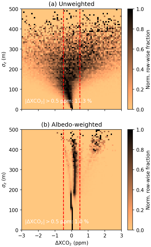
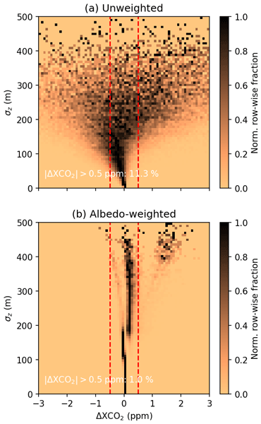
Figure 17 Normalized occurrence frequency of ΔXCO₂ for surface roughness values between 0 and 500 m using (a) the unweighted and (b) the albedo-weighted surface altitude. The frequencies in each row are normalized such that the maximum value is always one, for illustration purposes. The red dotted lines correspond to the accuracy requirement of ±0.5 ppm for CO2M (ESA, 2020).

Figure 17 compares the normalized distributions of ΔXCO₂ for surface roughness values between zero and 500 m when using unweighted and albedo-weighted averages of the surface altitude. The distributions of ΔXCO₂ get broader with larger surface roughness in both cases. The jump of ΔXCO₂ from slightly negative to slightly positive values for the surface roughness σ_z≳180 m comes most probably from remaining systematic changes for the usage of the albedo-weighted average over the mountains, as seen e.g. in Fig. 13f for the Mont Blanc region. However, this fact and the three branches seen starting from a similar surface roughness should be further analyzed in the future.

The vast majority of spatial samples do not exceed the accuracy requirement of 0.5 ppm (98.7 %) when using the albedo-weighted surface altitude. This fraction is smaller (88.7 %) when using the unweighted average. The broadening of the distributions occurs for smaller surface roughness values for the unweighted case.

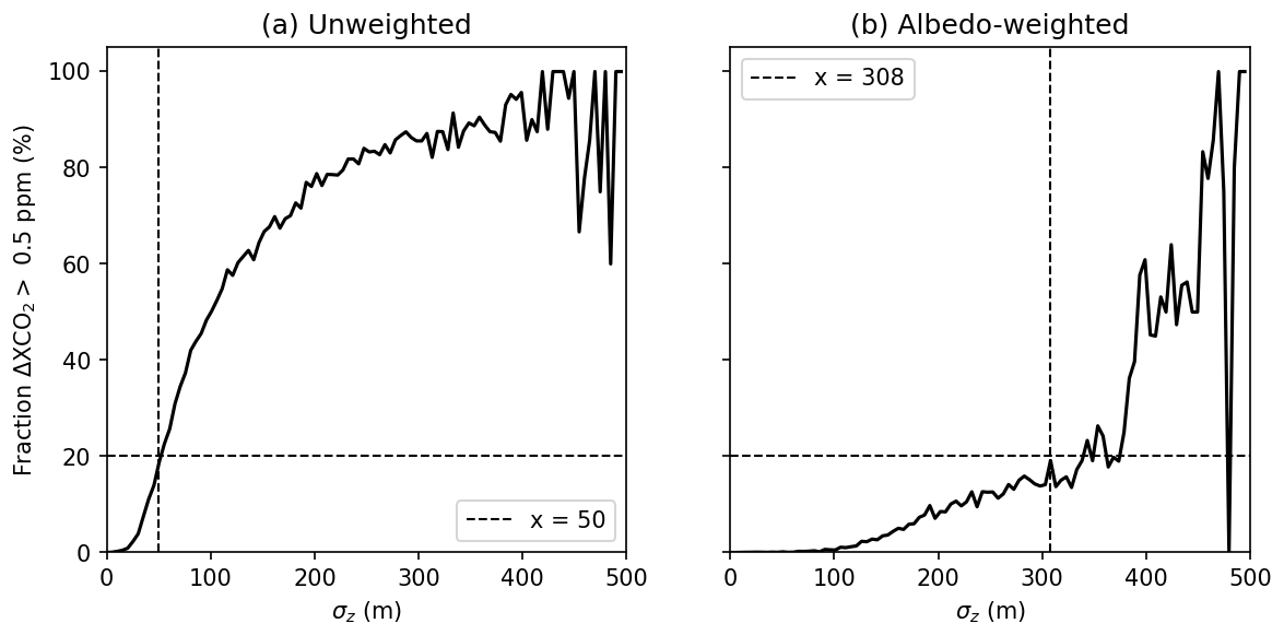
Figure 18 Percentage of XCO₂ errors larger than the accuracy requirement for CO2M versus the surface roughness for (a) unweighted and (b) albedo-weighted average of the surface altitude.

Therefore, it can be expected that surface roughness filter values can be relaxed when using the albedo-weighted surface altitude instead of the unweighted average. This is quantified in Fig. 18 where the fraction exceeding the 0.5 ppm requirement in each surface roughness bin is illustrated. This fraction is close to zero until σ_z=20 m (corresponding to about 20 % of global CO2M spatial samples over land) for the unweighted average case whereas it remains close to zero until 100 m in the case of using the albedo-weighted average. As another example, the figure also shows the surface roughness where it first exceeds the fraction of 20 %, which we use as an example for a better comparison. For the unweighted average this point is at σ_z=50 m whereas it is 308 m in the albedo-weighted case.

Thus, the results in this section suggest that the range of surface roughness values where trace gas retrievals can be applied can be extended when using the albedo-weighted average of the surface altitude instead of the unweighted average.

4.4 Relationship between albedo-weighted surface altitude and XCO₂

The previous results showed that the albedo-weighted averaged altitude decreases errors for heterogeneous scenes with subpixel variability in both surface albedo and altitude in idealized cases as well as in cases with real topography and albedo. However, the surface albedo can change over time, e.g. due to snow cover or seasonal vegetation changes, so that the surface albedo for the approach investigated in this study should be provided as close as possible to the measurement time. This is not possible in most cases because the albedo is not measured simultaneously with current instruments with the needed high spatial resolution. On the other hand, if the input surface altitude is known, it should be possible to apply the correction due to this effect as a post-processing step as soon as the albedo data are available for the measurement time. In the theory part of this study (Sect. 2), we used the average altitude as expansion point as an example, but the only assumption for the Taylor expansion is that the differences are small enough so that an approximation of first order is sufficient. The option for a post-processing correction is further investigated in this section. For this, we use the same regions as in Sect. 4.3 and create a simple formula that can be applied as post-processing in retrieval algorithms.

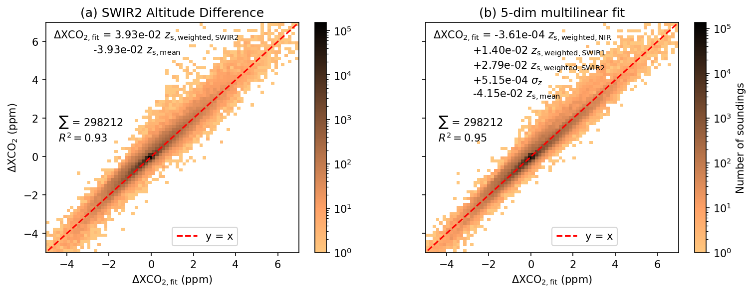
Figure 19 Two-dimensional histograms of the XCO₂ changes and fitting methods for all regions analyzed (see description in the text): (a) fitting linear regression of Δz_s in the SWIR2 band, and (b) fitting a linear combination of altitude changes, surface roughness and surface altitude. Only ΔXCO₂ values between −5 and 7 ppm are shown. Note the ΔXCO_2,fit corresponds to different fitting methods and also note the logarithmic color scale in each panel.

Figure 19 shows two methods of fitting the whole dataset. The first method is the method suggested by the real topography examples, which use the altitude change in the SWIR2 band to estimate the change in XCO₂. Although the slope of the linear regression in panel (a) is 0.04 ppm m⁻¹, consistent with the theoretical estimation in the introduction section, there seems to be a large spread in ΔXCO₂, which could be the result of missing parameters. Therefore, we investigate adding further input data and apply a multilinear regression using more variables to the dataset.

A multilinear regression with the albedo-weighted surface altitude in all three wavelength bands, the surface roughness σ_z and the mean altitude (panel b) shows that the altitude changes in the NIR have only a minor contribution to the overall changes. The SWIR1 and SWIR2 altitude changes contribute in a similar order of magnitude to ΔXCO₂ and the overall spread is reduced compared to the regression in panel (a). We also investigated using more variables for the multilinear regression, but did not find significant differences in the spread (not shown) so that we conclude that these five variables are sufficient to explain the majority of the XCO₂ changes. Note that the orange-colored bins in the histograms shown are single values and might not be relevant for the general retrieval success. Further variability most probably comes from the approximations made in the beginning of this study. We also tested applying a random forest approach using 14 input variables with similar results, and with the most important features being the albedo-weighted altitudes in the SWIR bands, as in Fig. 19.

Hence, we suggest the following post-processing equation that can be applied to XCO₂ retrievals with FOCAL-CO2M in order to account for the effect of albedo-weighted averaged surface altitude (see Fig. 19b):

$$\begin{array}{}\text{(30)}& \begin{array}{rl}\mathrm{\Delta }{\mathrm{XCO}}_{\mathrm{2},\mathrm{fit}}=& -\mathrm{3.6}\times {\mathrm{10}}^{-\mathrm{4}}{z}_{\mathrm{s},\mathrm{weighted},\mathrm{NIR}}\\ & +\mathrm{1.4}\times {\mathrm{10}}^{-\mathrm{2}}{z}_{\mathrm{s},\mathrm{weighted},\mathrm{SWIR}\mathrm{1}}\\ & +\mathrm{2.8}\times {\mathrm{10}}^{-\mathrm{2}}{z}_{\mathrm{s},\mathrm{weighted},\mathrm{SWIR}\mathrm{2}}\\ & +\mathrm{5.2}\times {\mathrm{10}}^{-\mathrm{4}}{\mathit{\sigma }}_z\\ & -\mathrm{4.2}\times {\mathrm{10}}^{-\mathrm{2}}{z}_{\mathrm{s},\mathrm{mean}}\end{array}\end{array}$$

with all values given in units of meters to get ΔXCO_2,fit in ppm. As a result, the post-processed XCO₂ is then calculated as:

$$\begin{array}{}\text{(31)}& {\mathrm{XCO}}_{\mathrm{2},\mathrm{postpro}}={\mathrm{XCO}}_{\mathrm{2},\mathrm{unweighted}}+\mathrm{\Delta }{\mathrm{XCO}}_{\mathrm{2},\mathrm{fit}}\end{array}$$

As ΔXCO₂ is dependent on the retrieval, this equation is only valid for FOCAL-CO2M, but the general methodology should be applicable to any retrieval algorithm. Note that Eq. (30) is only valid if all three bands are used to retrieve the greenhouse gas concentrations. If this is different, or if this correction should be used for other trace gases with wavelength bands other than the NIR, SWIR1 and SWIR2, another post-processing equation has to be derived since the albedo values will be different. Another option would be to use the albedo-weighted surface altitudes in the bias correction schemes of retrieval algorithms.

Some retrieval algorithm retrieve the surface pressure as part of the retrieval. Equation (30) can be converted to include pressure differences by first converting the $z_{\mathrm{s},\mathrm{weighted},i}$ values to their differences to the mean altitude $\mathrm{\Delta }{z}_{\mathrm{s},\mathrm{weighted},i}$ and subtracting the coefficient values from z_s,mean in Eq. (30):

$$\begin{array}{}\text{(32)}& \begin{array}{rl}\mathrm{\Delta }{\mathrm{XCO}}_{\mathrm{2},\mathrm{fit}}=& -\mathrm{3.6}\times {\mathrm{10}}^{-\mathrm{4}}\mathrm{\Delta }{z}_{\mathrm{s},\mathrm{weighted},\mathrm{NIR}}\\ & +\mathrm{1.4}\times {\mathrm{10}}^{-\mathrm{2}}\mathrm{\Delta }{z}_{\mathrm{s},\mathrm{weighted},\mathrm{SWIR}\mathrm{1}}\\ & +\mathrm{2.8}\times {\mathrm{10}}^{-\mathrm{2}}\mathrm{\Delta }{z}_{\mathrm{s},\mathrm{weighted},\mathrm{SWIR}\mathrm{2}}\\ & +\mathrm{5.2}\times {\mathrm{10}}^{-\mathrm{4}}{\mathit{\sigma }}_z\\ & +\mathrm{6.6}\times {\mathrm{10}}^{-\mathrm{5}}{z}_{\mathrm{s},\mathrm{mean}}\end{array}\end{array}$$

Each Δz in this equation can be converted to a pressure difference using the hydrostatic approximation for pressure:

$$\begin{array}{}\text{(33)}& \mathrm{\Delta }z=-H\cdot \mathrm{\Delta }\ln p.\end{array}$$

When retrieving the surface pressure in the NIR band, only, another possible way to get the dry-air column representative for the CO₂ column would be to use the retrieved NIR surface pressure and use the difference of the effective surface altitudes in the NIR and SWIR, converted to the pressure difference, to calculate the surface pressure in the SWIR. This new surface pressure can then be used to determine the dry air column which can be used to compute XCO₂.

4.5 Using albedo-weighted surface altitude as input or as post-processing

In the previous section, we developed an equation that can be applied in the post-processing of GHG retrieval algorithms to account for the effect of subpixel surface albedo changes. This might be necessary because the surface albedo is time-dependent, as discussed above, but it is measured by another satellite and not simultaneously. However, when assuming that we can get a good estimate of the surface albedo using climatologies, it might be better to use the albedo-weighted surface altitude directly as input to the retrieval, or more precisely, the meteorological parameters such as surface pressure, temperature etc. corrected for this altitude, as explained in Sect. 3.4. In this section, we analyze the differences that occur when using these two approaches.

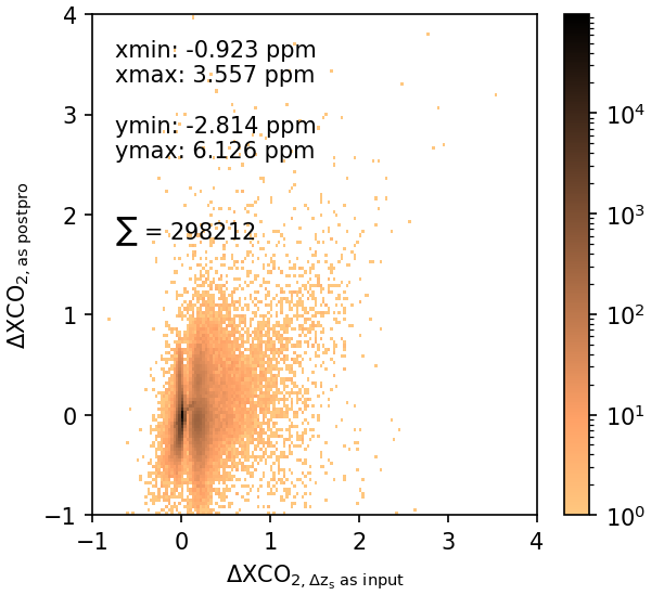
Figure 20 Deviation from 400 ppm when applying the post-processing given in Eq. (30) (y-axis) and using the albedo-weighted averaged surface altitudes in each wavelength band Δz_s directly as input for the retrieval (x-axis). Note the logarithmic color scale.

Figure 20 shows the deviations from the input 400 ppm for both methods as a histogram. Most ΔXCO₂ values are smaller than the required 0.5 ppm when directly using albedo-weighted surface altitude in the retrieval. The variability is slightly larger when applying the correction as a post-processing step using Eq. (31). There are more points exceeding 0.5 ppm when applying this post-processing procedure because it adds another approximation to those already outlined in Sect. 2.

In accordance with these results, panels (f) and (g) of the examples in Figs. 9, 11, 13 and 15 show that remnants of the surface altitude structure can be seen when applying the correction as post-processing which is not the case when using the albedo-weighted altitudes as input for the retrieval. The background variability in XCO₂ seems to be increased for Δz_s as input compared to using the post-processing equation, probably due to the noise in the S2 surface reflectance data, which then directly affects the retrieval results. This variability is on the order of 0.1 ppm, as seen in the example of Bełchatów (Fig. 9g) and the Rhine area in the Black Forest (Fig. 11g). As a consequence of the assumptions made when deriving the albedo-weighted surface altitude in Sect. 2, remaining errors in XCO₂ for high mountain areas (Fig. 13f) show systematic changes over the Alps. When applying the post-processing correction the XCO₂ changes are on the same order of magnitude (approx. ±2 ppm).

Table 3 Number of spatial samples, mean and median bias and the standard deviation (SD) for all regions and the three methods: Unweighted and albedo-weighted average of the surface altitude and after post-processing correction. APG stands for the whole dataset including the Alps, the Pyrenees and Germany.

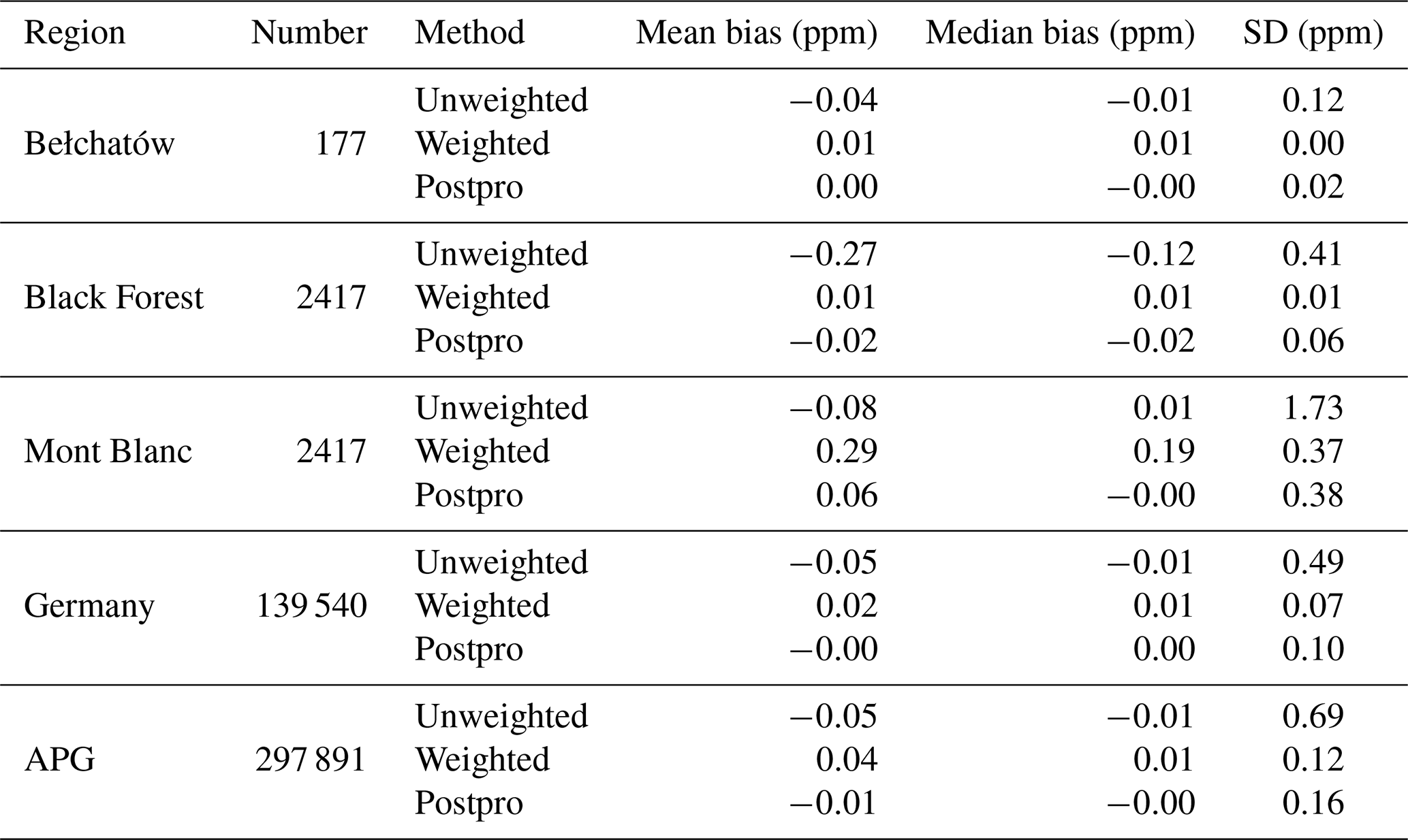
This is also reflected in the differences in the standard deviation of the ΔXCO₂ values of the dataset including spatial samples in Germany, the Alps and the Pyrenees as in the previous examples (Table 3) where the standard deviation of XCO₂ is reduced from 0.69 ppm with the unweighted average of the surface altitude to values smaller than 0.16 ppm using the other methods. When using the albedo-weighted surface altitude directly as input to the retrieval, the standard deviation is slightly smaller (0.12 instead of 0.16 ppm) as a result of the conclusions discussed above.

In addition, Table 3 shows statistics for all regions analyzed in this study. The median and mean biases are reduced for all regions, except for the Mont Blanc, where the mean bias is increases from −0.08 ppm (unweighted) to 0.29 ppm (albedo-weighted) for the reasons discussed in the previous sections. The standard deviations are reduced for the albedo-weighted and post-processing method compared to using the unweighted average. The standard deviations using the post-processing are slightly larger than using an albedo-weighted average directly in the retrieval.

Overall, the application as direct input to the retrieval removes the topographic structures from the retrieval results. In both the direct application and the post-processing, the variability of ΔXCO₂ is much smaller than in the case of using the unweighted average of the surface altitude (Sect. 4.2). Therefore, it can be concluded that both the direct application as input to the retrieval and the correction via the post-processing Eq. (31) lead to improved results compared to using the average surface altitude, so that the subpixel albedo in combination with the subpixel surface altitude should be accounted for in trace gas retrieval algorithms for passive satellite instruments using the sunlight reflected at the Earth's surface.

4.6 Dependence on size of the spatial samples

The degree of heterogeneity depends on the ratio of the observable objects and the size of the spatial sample. The subpixel variability of the albedo and the surface altitude might depend on the considered area. Thus, the size of the spatial sample could play a role in the magnitude of ΔXCO₂ and for the applicability of the post-processing correction to other satellites, which is investigated in this section. For this, we keep the basic methodology from Sect. 3.4 but create artificial spatial samples rectangular in latitude-longitude directions with different sizes for the Black Forest region.

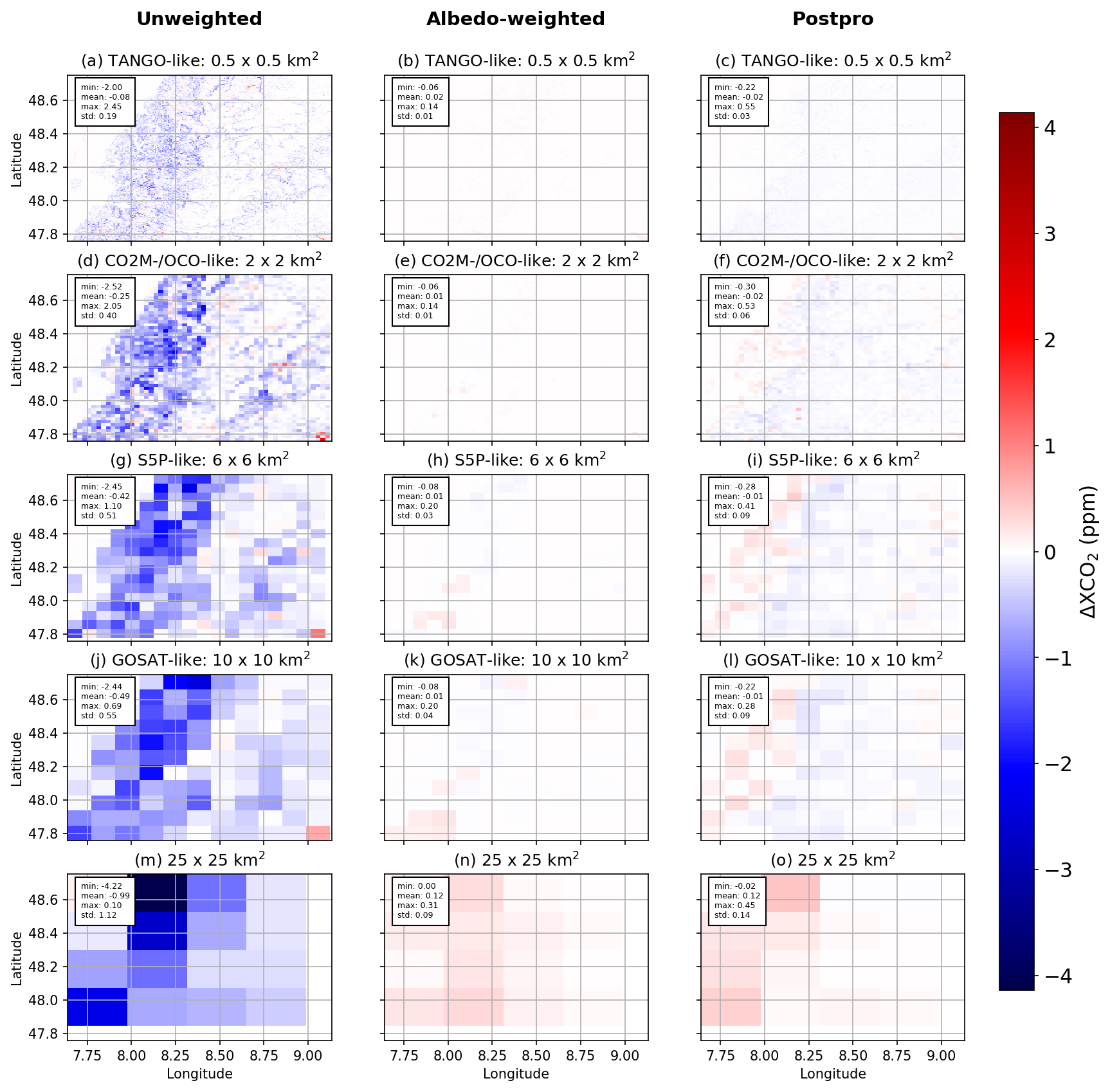
Figure 21 ΔXCO₂ values for spatial samples of different sizes, defined on a regular latitude-longitude grid, corresponding to the size in the title of each panel using the unweighted average (first column) and the albedo-weighted average of the surface altitude (second column) and after applying the post-processing correction (third column). The region shown is the Black Forest. Each panel includes the minimum, average and maximum values of ΔXCO₂ in the region shown. The titles of the panels indicate the spatial sample sizes that are closest to known Note that there are more examples in the Supplement of this study (Figs. S6 to S8).

The results for a selection of sizes can be found in Fig. 21 using the unweighted and albedo-weighted average of the surface altitude and after applying the post-processing correction using Eq. (31). The sizes of the spatial samples in these examples vary between 0.5 × 0.5 km² and 25 × 25 km². Further examples can be found in the Supplement of this study.

As can be seen in Fig. 21, the XCO₂ changes using the unweighted average increase with the size of the spatial samples. The differences to the true values of 400 ppm are usually a factor of four or more smaller when using the albedo-weighted average. In the case of the post-processing, the reduction of the bias is similar, but the structure of the mountains is still present in accordance with the previous results of this study, and the differences to the true values are slightly larger than when using the albedo-weighted average of the surface altitude for all shown spatial sample sizes.

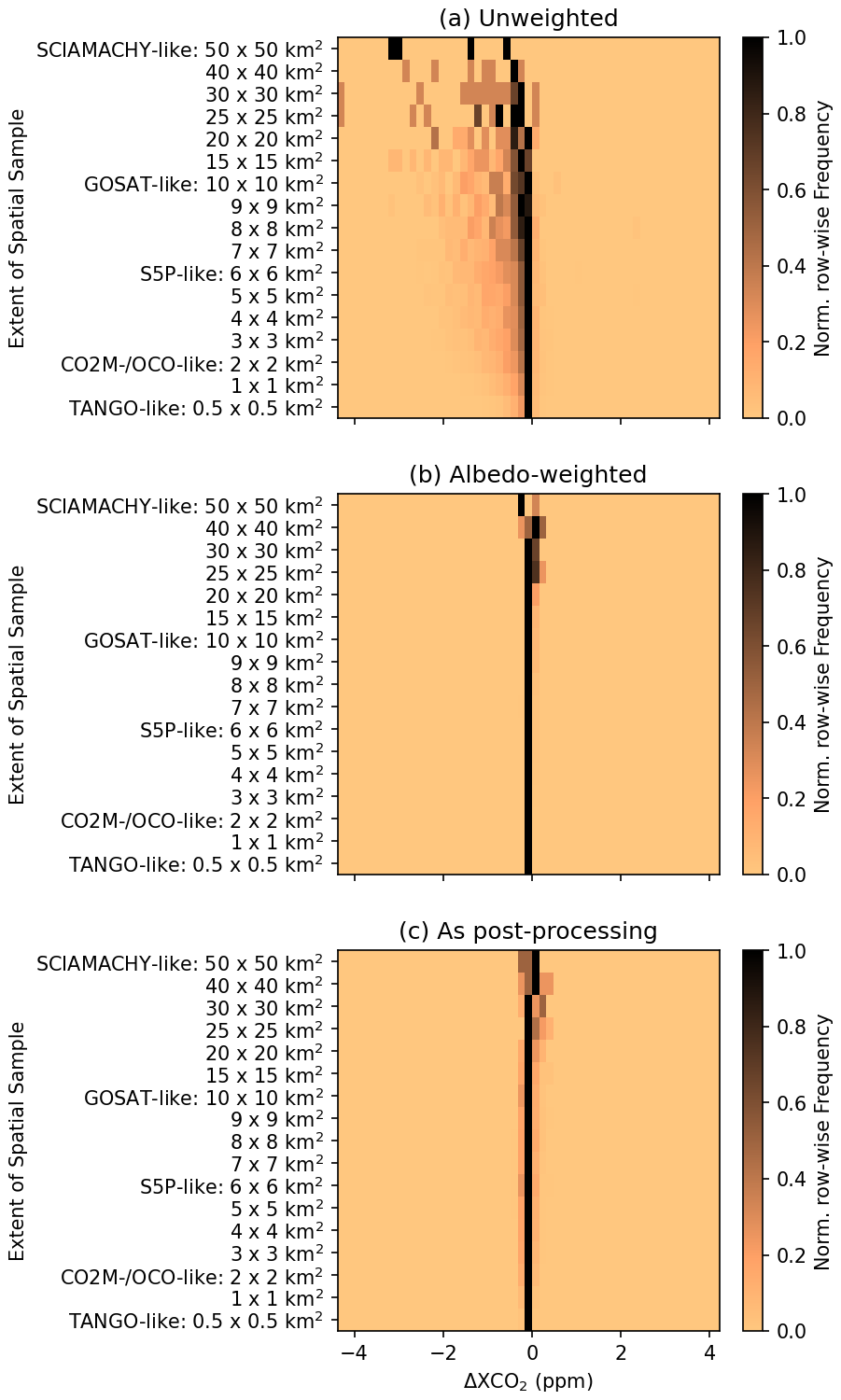
Figure 22 Normalized occurrence frequency of ΔXCO₂ values in the Black Forest region using the (a) unweighted and (b) albedo-weighted average of the surface altitude, and (c) after applying the post-processing equation.

This is confirmed in the normalized distributions for all analyzed spatial sample sizes in Fig. 22. The distributions show a significant fraction of ΔXCO₂ values exceeding 0.5 ppm for sample sizes of 2 × 2 km² and larger and the spread of the distributions increases with the size of the spatial samples when using the unweighted average of the surface altitude. In contrast, the 0.5 ppm threshold is not exceeded when using the albedo-weighted average, and is only exceeded for sizes larger than 30 × 30 km² when applying the post-processing equation. In general, the XCO₂ differences are slightly larger when applying the post-processing equation in comparison to the albedo-weighted average.

Therefore, it can be concluded from these results that the effect of using the unweighted average of the surface altitude increases with the size of the spatial samples, because the variability of surface altitude and albedo can be larger for larger spatial samples. In addition, the dependence of the post-processing equation on the size of the spatial sample seems to be small enough that it can be applied to other spatial samples that do not exceed a size of about 20 × 20 km².

5 Conclusions and discussion

In this study, we investigated an error source related to correlated subpixel variability of both surface albedo and surface altitude for passive satellite instruments that use measured spectra from the sunlight reflected from the Earth's surface for trace gas retrievals. Based on linearized theory starting from a one-wavelength Lambert-Beer law, we found that the subpixel surface altitude should be weighted by the surface reflectance (albedo) to get the effective surface altitude that is representative for the light path of the instrument's spatial sample on the ground. One main assumption was that the altitude dependence of the dry-air column-averaged mole fraction in the lowest parts of the atmosphere, where the profile is cut or extended, is small and, to a lesser degree, that extending/cutting the meteorological profiles is a valid assumption. We set up a methodology using Copernicus Sentinel-2 data combined with Copernicus DEM data and the FOCAL greenhouse gas retrieval algorithm in a self-consistent configuration by generating a database of spectra with FOCAL to test the impact of using an albedo-weighted average of the surface altitude in the three wavelength bands that will be measured by the future CO2M satellite mission.

We started applying the method first to artificial examples with well-defined conditions. They consisted of a spatial sample split into two parts with different user-defined albedo and altitude values and area fractions. We found that there is a non-linear dependence on the fraction and the albedo pairs used and that there is an altitude dependence of the retrieved XCO₂ changes that is different across the wavelength bands of CO2M. The changes in the SWIR1 band were generally smaller than in the SWIR2 band. Altogether, the XCO₂ changes were largely reduced when using the albedo-weighted average of the surface altitude in the retrieval which is consistent with the theoretical derivation.

In order to see the magnitude of differences due to this effect for typical real scenes, we then applied the methodology to real topography showing examples of the Bełchatów power plant in Poland, the Black Forest in Germany, the Mont Blanc area and the whole country of Germany. We found differences in XCO₂ that are larger than the accuracy requirements of 0.5 ppm for the CO2M mission when using the unweighted subpixel average of the surface altitude as done in many trace gas retrieval algorithms. We note that although 0.5 ppm was used in this study, the actual error budget for heterogeneous scenes and surface pressure is only part of the total accuracy and on the order of 0.2 ppm (Buchwitz et al., 2020). These differences are generally reduced to values smaller than the requirements when using the albedo-weighted average of the surface altitude, apart from high-altitude samples over the Alps, where the approximations of the linearized framework no longer hold. Therefore, the examples with real subpixel topography and subpixel albedo confirmed that using the albedo-weighted averaged surface altitude has the potential to reduce biases in the retrieval. As a consequence, the results also showed the potential to relax pre-processing filter parameters connected to the surface roughness.

In addition, we investigated the possible application of this correction in the post-processing because the subpixel albedo composition is usually measured with another instrument and might be provided at a later time. We found that a multilinear regression with the albedo-weighted surface altitudes in all three wavelength bands, the surface roughness and the average altitude is sufficient to account for the majority of the variability, but leaves remnants of the orographic features which do not occur when using the albedo-weighted average of the surface altitude directly as input for the retrieval (or more precisely the meteorological parameters such as surface pressure, temperature etc. corrected for this altitude). This could be further investigated, for example by using symbolic machine-learning to derive an equation that improves the fit of Fig. 19, or by using the albedo-weighted altitudes as part of the bias correction in the retrieval algorithm, both of which are beyond the scope of this study. In FOCAL-CO2M, the bias correction is based on machine-learning so that the albedo-weighted altitudes could be additional features to be considered there. It should be noted that the bias corrections of current greenhouse gas retrieval algorithms might account already for parts of this effect when using surface altitude, surface pressure or retrieved albedo as input and probably some measure of the inhomogeneity within the spatial sample.

Finally, we investigated how the error due to using the unweighted average of the surface altitude varies with the size of spatial samples and found that the error increases with the sizes, but remains smaller than 0.5 ppm for sizes smaller than 20 × 20 km² when either directly using albedo-weighted surface altitude or when applying the post-processing correction.

The method applied in this study is not limited to FOCAL-CO2M, but can be applied to any retrieval algorithm using reflected radiances. It could also help to improve biases in other trace gas retrieval algorithms. The results using the FOCAL-CO2M algorithm indicate that the subpixel surface reflectance is a crucial parameter for satellite observations.

The results of this study showed the effect with the example of retrievals of XCO₂. Similar relative effects can be expected for XCH₄. The conclusions are not limited to greenhouse gases, which are used as an example here, but in principle they apply to any trace gas that is retrieved from reflected radiances. It might not even be limited to reflected radiances but similar effects might occur from retrievals of trace gases from thermal emission radiances, which is out of the scope of this study. On the other hand, as the requirements for greenhouse gas measurements from satellites are stringent (in the order of 0.5 %), this effect is especially relevant for CO₂ and other greenhouse gases.

Many assumptions have been made for this study. Apart from the approximations done in the theoretical derivation (e.g. non-scattering isothermal atmosphere, Lambertian surface and small altitude variability), we assumed here that the Sentinel-2 data are the true albedo values, but they include errors which should be accounted for when applying the method to real satellite data, e.g. by providing an uncertainty for the effective altitude which can then be added to the XCO₂ uncertainty. Furthermore, the Sentinel-2 spectral bands do not exactly match the wavelength bands measured by CO2M. However, the available bands and their data sets cannot be changed. Therefore, this adds to the uncertainty in using Copernicus Sentinel-2 data as a proxy for the real surface reflectance at the CO2M wavelength bands. In addition, the co-location of the DEM and albedo data is an important parameter, because any error in this will have direct effect on the XCO₂ estimate, especially at subpixel neighbor locations with highly heterogeneous conditions. We also assumed that each subpixel contributes equally to the signal on the detector while, in reality, the illumination depends on the point spread function and the bidirectional reflectance distribution function and might be different in the center and at the edges of the detector pixel. Furthermore, there are still remnants of altitude-dependent features when using the albedo-weighted average of the surface altitude, so that further analysis should be done in the future to remove these features. In addition, we did not account for mountain slopes and the resulting anisotropy of the reflectance at any point in this study, which should be further investigated in the future.

This study is based on a selection of regions in Europe. In order to see the global effect, a global map of co-located surface altitude and albedo values in the respective wavelength bands is needed, or simultaneous measurements of these quantities and the spectra for the trace in the same satellite geometry. A calculation of a global albedo map based on the S2 data and its application to real satellite measurements is subject for a future study. In addition, the spatial coverage of the S2 data is important because it depends on cloud-free and low-aerosol scenes. Therefore, single overpasses close to the XCO₂ measurement time might be sufficient e.g. in desert regions whereas averages over months might be needed over regions with many cloudy days.

We used heterogeneity of the surface altitude as a proxy for heterogeneity of the dry-air column which then affect XCO₂. If there is heterogeneity in the CO₂ concentration itself on a subpixel scale, the effect will be the same. For example, if there is a local power plant with large albedo downwind and low albedo upwind, it can be expected that, in principle, the CO₂ concentration has to be weighted with the albedo to get the correct results from the greenhouse gas retrieval.

Altogether, it can be concluded from this study that there are strong indications that the albedo-weighted average of the surface altitude should be considered for retrievals of the trace gas concentrations from passive satellite instruments using sunlight reflected at the Earth's surface as the source of information. Ideally, the albedo should be measured simultaneously and with high-resolution co-located with the trace gas measurements in the respective wavelength bands. The results using the self-consistent setup suggest that accounting for this effect can be done either directly as input to the retrieval or as a post-processing step by applying a post-processing equation as done for FOCAL-CO2M in this study or by adding the surface altitude weighted by the subpixel albedo values to the bias correction schemes of trace gas retrieval algorithms. The method substantially reduces one specific component of terrain-related XCO₂ bias and may be valuable for future retrieval development, but its operational benefit remains to be demonstrated under realistic measurement and forward-model uncertainties which is the subject for a future study.

Appendix A: Impact of scattering

The scattering parameters used in this study (optical thickness, pressure and Ångström coefficient of the scattering layer) are based on the dataset used in Weimer et al. (2025). The dataset consists of one year of data representative for CO2M. Here, we use the average retrieved optical thickness of the scattering layer (τ_sca=0.019). Pressure and Ångström coefficient are taken at the same sounding where this average occurs.

We applied our method also to data without scattering and a scattering optical thickness as average plus two standard deviations, see Fig. A1. The results without scattering are similar to the average scattering optical thickness (note that this is not the aerosol optical thickness) with an R²=0.97, which is larger than the R² for the data originally use for fitting the data (see panel b).

On the other hand, if the atmospheric scattering is increased significantly, the retrieval of XCO₂ might become difficult. This is shown in Fig. A1c where the scattering is increased to τ_sca=0.037. The R² value is reduced to 0.57 in this case and the scatter shows spikes around $\mathrm{\Delta }{\mathrm{XCO}}_{\mathrm{2},\mathrm{fit}}=\mathrm{0}$. These spikes are a result of homogeneous samples with small average albedo included in the dataset which we tested by removing homogeneous scenes using thresholds of 10 m for σ_z and a minimum standard deviation of the albedo of 0.02. If these samples are excluded from the data, the R² value is increased to 0.7 (not shown).

To summarize this section, Eq. (30) is also applicable to cases without scattering in the atmosphere, but not if the scattering optical thickness is increased to τ_sca=0.037. A more comprehensive study varying all scattering parameters would be needed to confirm that the equation is also applicable to a wide range of scattering regimes.

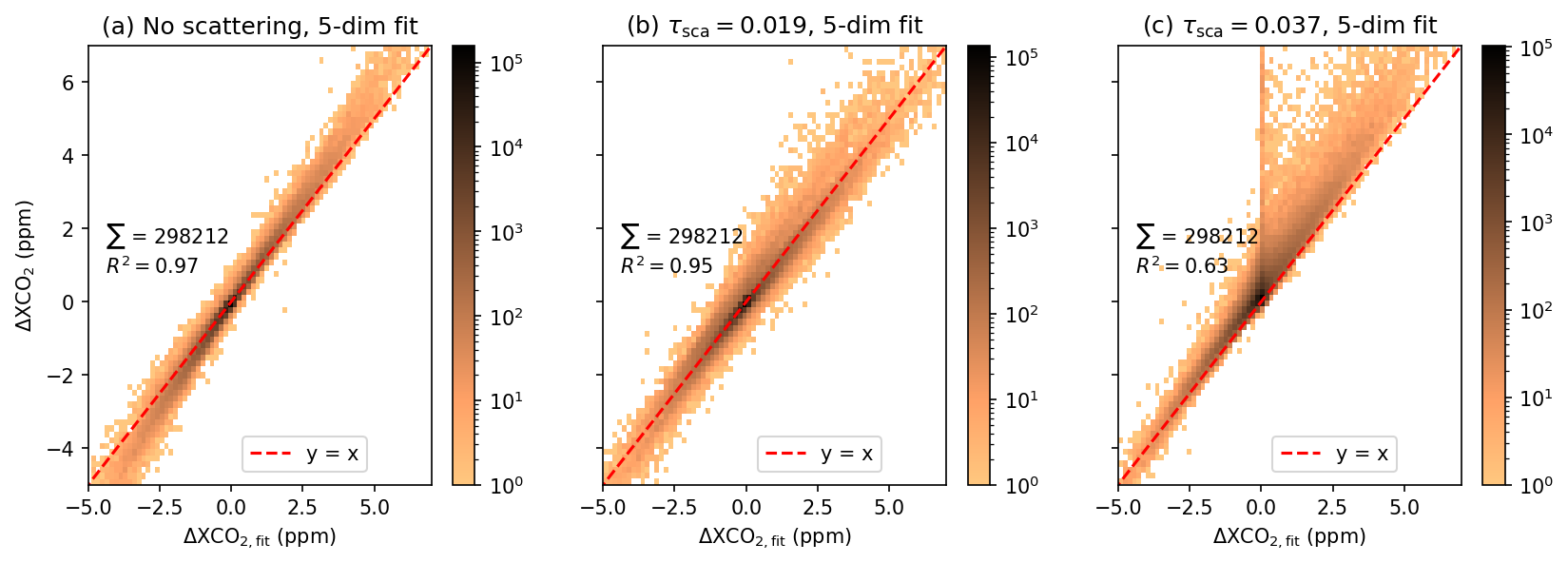
Figure A1 Estimation of ΔXCO₂ using Eq. (30) for the whole dataset with (a) no scattering, (b) an optical thickness of the scattering layer of τ_sca=0.019 and (c) average plus 2 times standard deviation of the retrievals by Weimer et al. (2025): τ_sca=0.037. The other scattering parameters (pressure and Ångström coefficient of the scattering layer) have been taken from the same retrieved spatial sample as τ_sca. Only ΔXCO₂ values between −5 and 7 ppm are shown. Note the logarithmic color scales in each panel.