A novel segmentation algorithm for the ARM user facility all-sky imagers using machine learning applications

Clouds play a pivotal role in modulating the Earth's energy budget through the reflection of incoming solar radiation and the trapping of outgoing longwave radiation. Ground-based all-sky imagers offer an objective assessment of cloud cover and can be used to estimate solar irradiance, classify cloud types, track cloud movement, and serve as a benchmark for the evaluation of satellite and reanalysis data products. The Atmospheric Radiation Measurement (ARM) user facility has utilized all-sky imagers for more than 25 years to monitor cloud cover and augment its comprehensive suite of atmospheric measurements. Following the retirement of its Total Sky Imager (TSI), ARM recently deployed the TSI's successor, the All-Sky Imager (ASI-16 camera systems). To provide a smooth transition and continuity to the vast amount of knowledge gathered by the TSI over the years, while addressing typical deployment issues, we developed a novel pixel segmentation algorithm, the ASI Sky Cover (ASISKYCOVER). ASISKYCOVER builds on the different strengths and properties of the TSI processing algorithm while integrating machine learning techniques, ensuring data validity and accuracy across diverse atmospheric conditions. It enhances cloud cover characterization with new features such as artifact detection and uncertainty quantification. ASISKYCOVER also includes cloud cover estimates for near-zenith (narrow field-of-view) and reduces susceptibility to false detections. This study introduces ASISKYCOVER, details its algorithm framework, and demonstrates its capabilities using a year-long dataset from the ARM Southern Great Plains site. A comparison with co-located TSI data tentatively suggests that the dominant cloud type per scene might be the best predictor of inter-consistency between cloud detection algorithms. This ASI-TSI comparison and evaluation against other ARM measurements, such as zenith-pointing radars and lidars underscores the ASISKYCOVER's potential to improve cloud cover analyses and data evaluation efforts, as well as to be integrated into higher-level data products that synergize instrument suites to generate new and insightful information.

1 Introduction

Clouds modulate the atmospheric energy budget by reflecting part of the incoming solar shortwave radiation back to space and partially emitting outgoing longwave radiation back towards the surface (greenhouse effect). The exact contribution of clouds to the energy budget depends on their microphysical properties and their coverage, the characterization of which is still deficient (e.g., Grosvenor et al., 2018; Loeb et al., 2018).

Satellite data products provide a comprehensive long-term cloud cover record but suffer from biases in characterizing near-surface and optically thin high-level clouds, and are generally challenged above ice surfaces (e.g., Kato et al., 2012; Maahn et al., 2014; Minnis et al., 2008). Moreover, while geostationary satellites provide samples at a high temporal resolution at small spatial scales, they are confined to low- to mid-latitudes (typically below ∼50°), rendering a paucity of high-latitude cloud cover data.

Ground-based measurements complement, and in some cases, replace satellite data for certain purposes, such as multi-scale process understanding. These measurements provide a wealth of information, which, although local, is typically of high accuracy and value, especially for validating satellite products. For example, ground-based all-sky imagers can offer an objective assessment of cloud cover surrounding deployment sites using various algorithms (e.g., Esteves et al., 2021; Li et al., 2022; Sarangi et al., 2025). Imager-based data products can be used to estimate solar irradiance (e.g., Logothetis et al., 2022; Manandhar et al., 2023; Park et al., 2021; Pfister et al., 2003; Song et al., 2022), classify cloud types (e.g., Buch and Sun, 1995; Calbó and Sabburg, 2008; Wang et al., 2020), track cloud movement (e.g., Raut et al., 2023), and serve as a benchmark for the evaluation of satellite and reanalysis data products (e.g., Ackerman and Cox, 1981; Werkmeister et al., 2015), as well as other ground-based cloud cover estimates (e.g., Kassianov et al., 2005; Riley et al., 2020). Moreover, when considerations of the camera frame of reference equivalent to surface visual observers are made (see Long et al., 2006), all-sky image records can be combined with historical records of fractional sky coverage made by human observers (e.g., Free et al., 2016) to generate long-term climatology extending back to well before the satellite era (Free and Sun, 2013).

The ARM user facility has been operating all-sky imagers for a quarter of a century to characterize cloud coverage and supplement its other measurements. Specifically, the total sky imager (TSI; Morris, 2005) was used throughout this period until the recent retirement of all TSI instruments. Two TSI instruments at the ARM Southern Great Plains site in Oklahoma (SGP; Sisterson et al., 2016) and the Eastern North Atlantic central site at Graciosa Island (ENA; see Mather, 2024; Wood et al., 2015) continued to be operated alongside the TSI successor, the All-Sky-Imager (ASI-16; Schreder-CMS, 2017), for evaluation and data continuity purposes, as discussed below, until their decommission in August and July of 2025, respectively.

The TSI's advanced cloud cover algorithm (Long et al., 2006) provides a reliable cloud cover data product in an extra wide field-of-view (FOV) covering the sky up to 80° off-zenith. The data product includes an error mitigation routine and a unique feature of correcting the estimated cloud cover from the projected image sensor to an observer's frame of reference, facilitating robust comparisons with historical records. This analytical correction renders the cloud cover algorithm significantly more computationally efficient than other methods that perform this correction via various image distortion corrections.

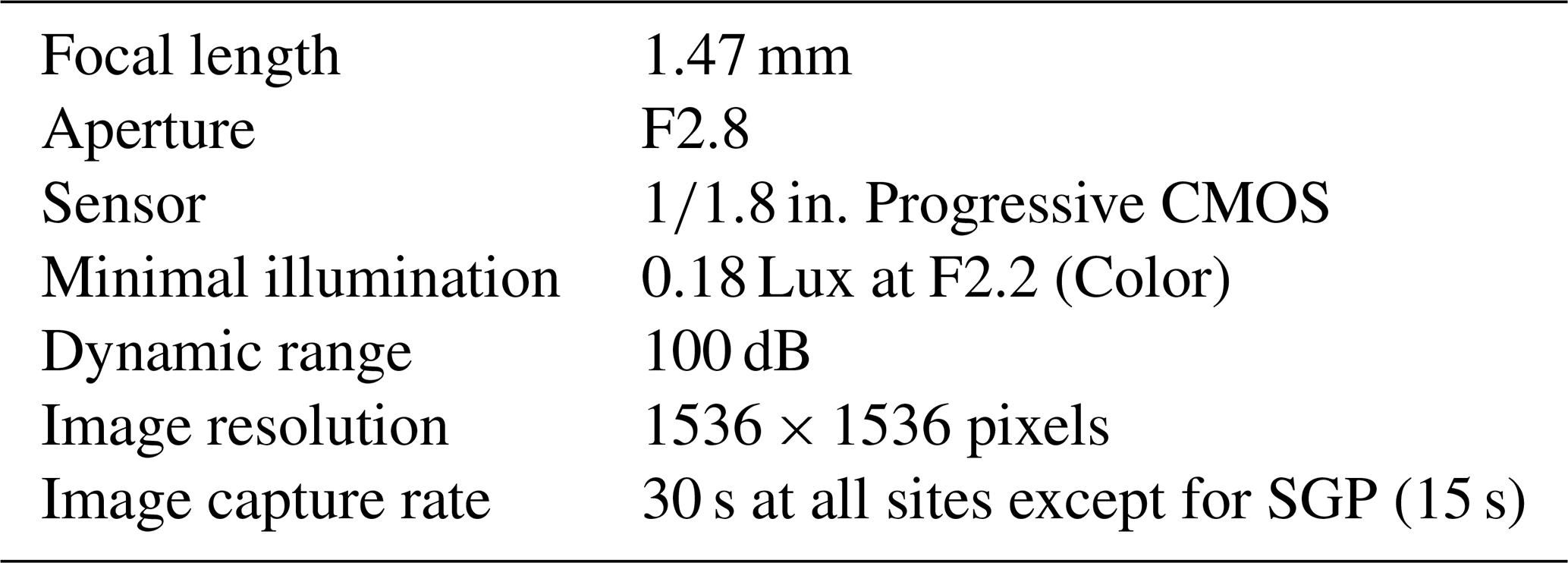
Unlike the TSI, its successor, the ASI (Fig. 1), has no moving parts and operates a Complementary Metal-Oxide-Semiconductor (CMOS) sensor, which is less prone to saturation and flaring effects than charge-coupled device (CCD) sensors, such as the one operated by the TSI, resulting in a higher dynamic range in pixels surrounding bright objects such as the solar disk, which renders a mechanically rotating shadowband obsolete (see Table 1 for ASI specifications).

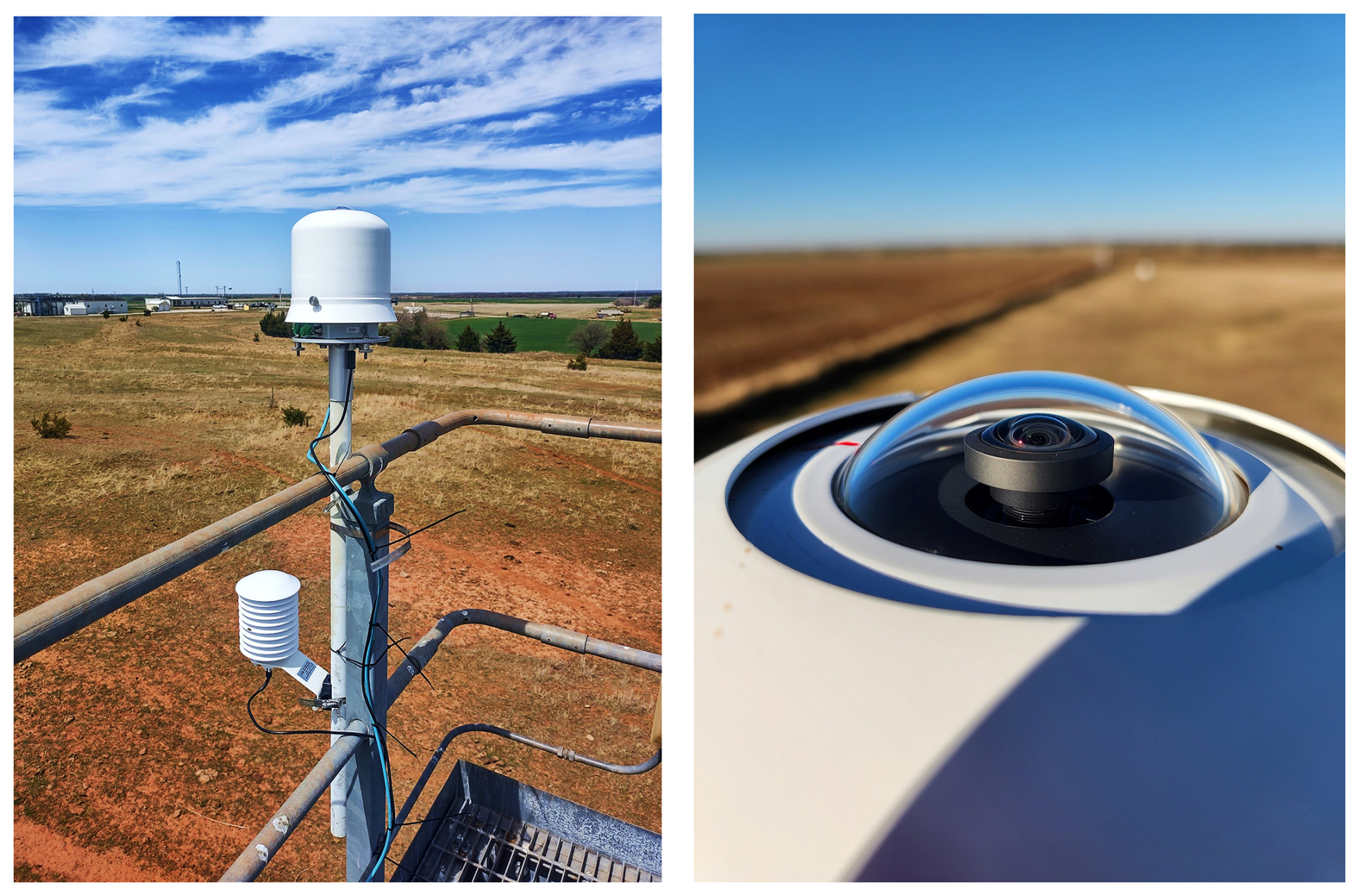
Figure 1 (Left) The ARM All-Sky-Imager (ASI) mounted at the Southern Great Plains (SGP) central site and (right) zoom on the ASI housing and fish-eye lens.

Table 1 The ARM ASI specifications.

The ASI vendor-provided image processing software allows for some control over the partitioning of cloudy and clear sky areas in the ASI image by setting specific thresholds. However, because different sky scenes (midday, sunset, partial solar disk coverage, polluted days, etc.) generate different variations and contrast between the RGB channels and channel ratios of clear and cloudy pixels, fixed thresholds are unsuitable for an operational product aimed at applying to the diversity of atmospheric scenes typical to different ARM deployments throughout the year. Moreover, the ASI vendor-provided software does not offer features critical to the dynamic nature of ARM sites and deployments, such as automatic determination of the effective image center and border, solar disk characterization, and evaluation of ASI camera misalignment and time-dependent offsets.

Here, we present an advanced machine-learning-powered cloud cover data product, the ASI Sky Cover (hereafter, ASISKYCOVER). The ASISKYCOVER product is consistent with the TSI processing algorithms in many aspects, such as the extensive solid angle coverage and processing of cloud cover to represent the camera (visual observer) position's frame of reference. However, this product provides essential upgrades to ensure more accurate diagnostics and reduced susceptibility to false detections. It offers new features such as artifact detection, uncertainty metrics, and the estimation of near-zenith cloud cover, facilitating direct comparisons with remote-sensing datasets and streamlining cloud cover evaluation, as well as the synergistic use of ASI data with other zenith-pointing ARM measurements, including radar, lidars, and radiometers.

In the following sections, we describe the ASISKYCOVER processing algorithm (Sect. 2) and present an analysis of the ASISKYCOVER output for the entire year of 2024 at the ARM SGP site, along with a comparison to the co-located TSI, radar, and ceilometer instruments. Conclusions and a short outlook are given in Sect. 4.

2 Methodology

The ASISKYCOVER algorithm comprises multiple steps, including image preprocessing and site-dependent correction, a machine learning (ML)-powered pixel segmentation algorithm, segmentation post-processing, and an ML-powered solar disk state classification algorithm. Those components are described below.

2.1 Image Preprocessing and Deployment Site Configuration and Corrections

Before applying the ASISKYCOVER segmentation algorithm, ASI images require minimal preprocessing to determine the effective (circular) image center and edges. This processing step is essential since the effective position of the image can influence the cloud cover calculation as a result of inaccurate representation of the projected sky area represented by a given pixel (see Sect. 2.3). Slight deviations in image center and edge coordinates are expected between ASI units, given the exact positioning of the ASI housing relative to the ASI's CMOS sensor (see Fig. 1). While such a property is essentially fixed for a given unit, slight deviations can occasionally occur (e.g., as a result of strong winds). Therefore, the image center coordinates, x_c and y_c, are determined for individual images by finding the x-axis index corresponding to the maximum y-axis image diameter, and vice versa. Edges are determined by finding “near-black” pixels, i.e., pixels with red-green-blue (RGB) brightness values near 0 (on an integer scale of 0 to 255).

With this method of determining the effective image edges, ASI site deployment misalignment can be characterized in preparation for the segmentation task. Assuming that the ASI position (in azimuth and zenith) is fixed throughout a given deployment, instrument misalignment needs to be characterized only once. In the event of a unit position change or in cases where there is an interest in reevaluating the unit's alignment, multiple characterization cycles must be applied. Note that, unlike sky imagers with a shadowband or arm, such as the TSI, solar zenith angle (SZA) and azimuth angle biases are generally more challenging to determine by visually inspecting a given image.

To determine the SZA and azimuth angle biases, the center of the solar disk is manually identified in a set of images where it is visible, preferably from different times of day. Automated algorithms to detect the solar position exist in the literature (e.g., Savoy et al., 2016). However, the errors associated with such algorithms are ostensibly greater than those with manually annotated images, mainly because of the requirement for clear-sky images combined with field-deployment constraints (e.g., dirt on the camera, cases of which were tested but not shown). Combined with the fixed nature of ARM deployments, which eliminates the need for frequent revaluation of solar position misalignment, we find that the manual labeling approach is best suited for this task.

Following this manual identification of the solar disk center, we use astronomical factors and site coordinates to calculate the azimuth angle (ϕ) and SZA (θ) corresponding to the time of each of the annotated images. Under an equidistant projection assumption, we can analytically convert those angles (in units of radians) to pixel coordinates x and y using:

$$\begin{array}{}\text{(1a)}& {\displaystyle }x=x_c+r\sin \left(\mathit{\varphi }+\mathit{\pi }\right)=x_c-r\sin \left(\mathit{\varphi }\right)\text{(1b)}& {\displaystyle }y=y_c+r\cos \left(\mathit{\varphi }+\mathit{\pi }\right)=y_c-r\cos \left(\mathit{\varphi }\right),\end{array}$$

where r is the radial distance of the calculated solar position from the effective image center, which is given by:

$$\begin{array}{}\text{(2)}& r={\displaystyle \frac{r_{\mathrm{eff}}}{\mathit{\pi }/\mathrm{2}}}\cdot \mathit{\theta },\end{array}$$

where $r_{\mathrm{eff}}=d_{\mathrm{eff}}/\mathrm{2}$ is the effective image radius (d_eff being the effective image diameter). Pixel zenith and azimuth angles from the manually annotated solar disk center x and y coordinates can be calculated using the inverse forms of Eqs. (1) and (2). The shift of ϕ by a factor of π in the trigonometric functions in Eq. (1) stems from the upward-looking ASI geometry, which, unlike maps or nadir-pointing satellite imagery, results in an apparent east-west mirroring and a north-south flipping. This different geometry means that when ASI images are shown with the north direction at the top, the east direction (and hence, sunrise, for example) will be located at their left part, unlike the common intuitive interpretation of such images, where the east direction is to the right of the north. We also note that while an equidistant projection is a specialized form of barrel distortion, we do not apply other barrel distortion corrections, given the ASI lens's relatively minor distortion values, smaller than 0.3 %, 0.8 %, 1.9 %, and 3.8 % at pixel elevation angles of 60, 70, 80, and 90°, respectively, based on tables provided by the ASI vendor (cf. Long et al., 2006, their Fig. 5). These small distortion values essentially translate to cloud cover errors of a fraction of a percentage point, much smaller than the typical scene uncertainty (see Sects. 2.3 and 3.1).

Using the Pixel zenith and azimuth angles, corresponding to the manually annotated solar disk center, and their deviations from the calculated SZA and azimuth angle, the site-specific biases of those angles are determined as the average deviation in the annotated image subset. The standard deviation metric calculated from the annotated image subset serves as a measure of robustness in bias characterization. Based on that metric, the positioning biases observed across different ARM deployments are robust, as indicated by the standard deviation of the differences between the annotated and calculated angles, typically on the order of 1° or less (not shown). For the SGP central site analyzed here, these biases are relatively small at $-\mathrm{0.23}\pm \mathrm{1.51}$° and 2.69±1.34° for the solar azimuth and SZA, respectively (e.g., compare the positions of the yellow and green circles in Fig. 2d to g).

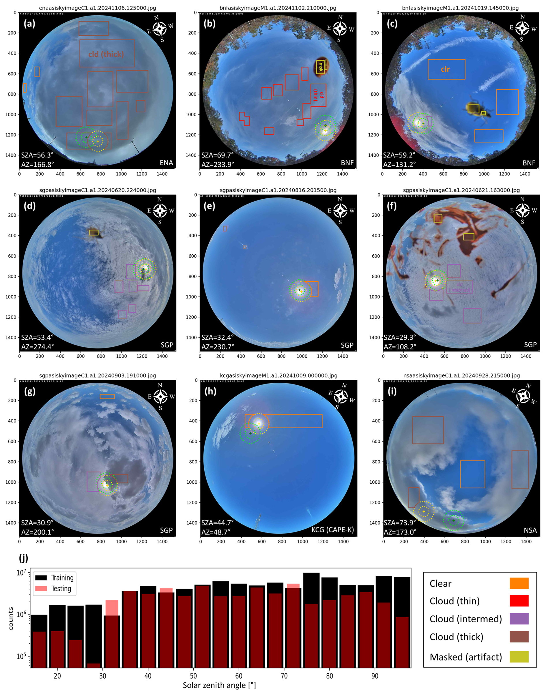
Figure 2 (a–i) Examples of images from different ARM deployments with manually labeled sectors of clear (orange), thin clouds (red), intermediate-thick clouds (purple), thick clouds (brown), and artifacts (masked; yellow), which are included in the training dataset (see legend and a selected set of in-box labels). In the depicted images, the x- and y-axis values represent pixel indices. The compass rose at the top right of each panel denotes the location of the north, south, east, and west directions, with compass tilting reflecting the site-specific solar misalignment. (Note that the ASI images appear mirrored in the east-west direction; see Sect. 2.1 for details.) The concentric green and yellow circles designate the analytically calculated and misalignment-corrected solar disk positions, respectively (outer circle radius of 100 pixels). Solar zenith and azimuth angles are shown at the bottom left corner of each image. The corresponding ARM deployments are shown at the bottom-right of each panel (ENA – Eastern North Atlantic; BNF – Bankhead National Forest; SGP – Southern Great Plains; KCG – Cloud And Precipitation Experiment at Kennaook; NSA – North Slope of Alaska). (j) Distribution of training (black) and testing (red) pixel samples as a function of solar zenith angle (SZA; bin size of 2°).

Finally, the ASISKYCOVER algorithm can utilize deployment masks that can be manually generated to exclude fixed objects visible in pixels within its effective FOV (80° off-zenith) used in the cloud cover calculations, if such objects exist in a given ASI deployment. The SGP central site deployment, however, is clear of such obstructing objects within the ASI FOV, and therefore, a mask is not applied in this case. In deployments with obstructing objects (e.g., the masked antenna at the top of Fig. 3a), the masked pixels are excluded from the cloud cover calculation but are considered in the cloud cover uncertainty calculation discussed below (see Sect. 2.3).

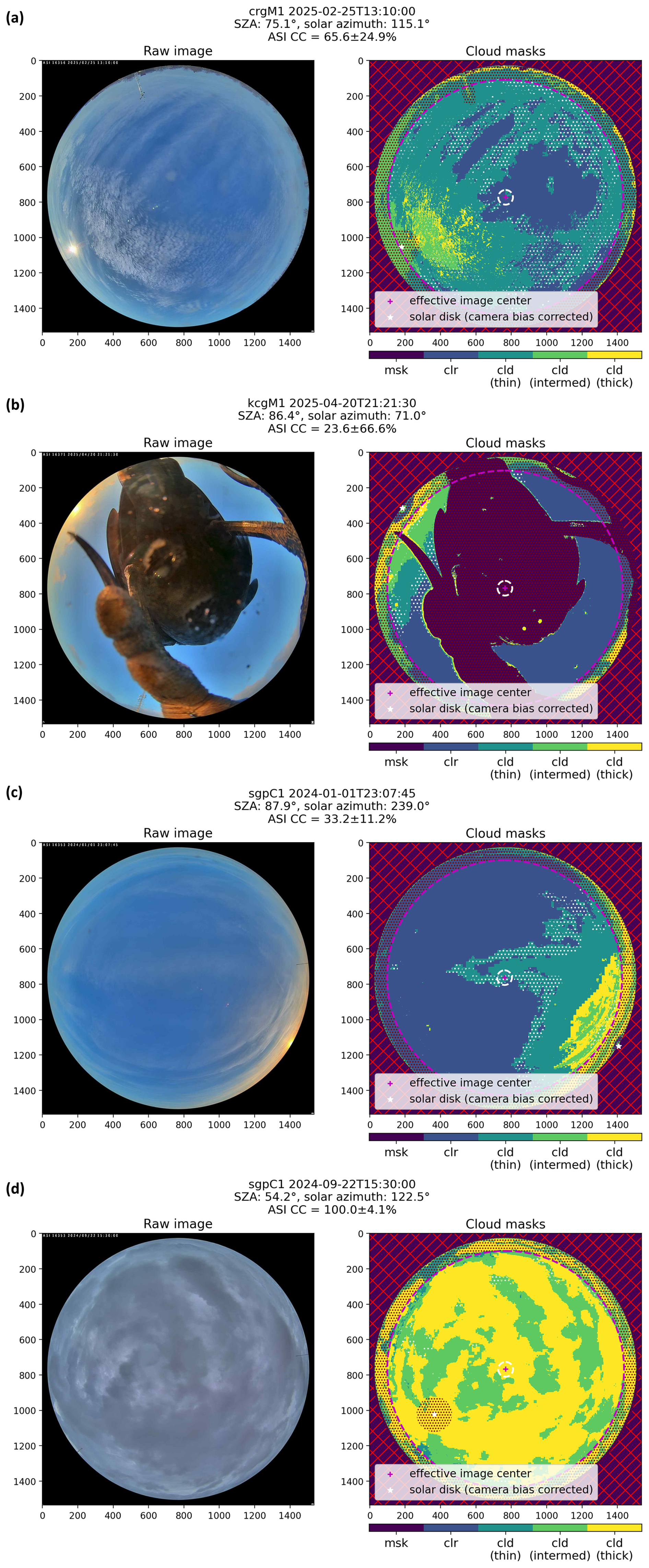
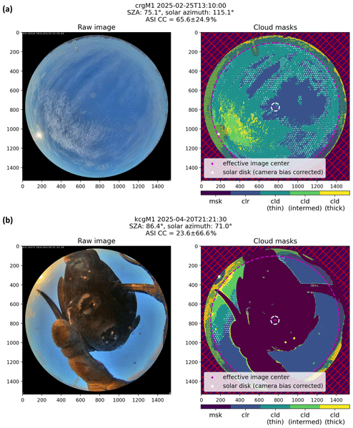
Figure 3 ASISKYCOVER pixel segmentation algorithm output for selected scenes. (Left) Raw ASI image (note that the ASI images appear mirrored in the east-west direction; see Sect. 2.1 for details), (right) algorithm output. The resolved classes are given in the legend at the bottom of the classification masks. In each classification mask, the red “+” denotes the determined image center, the dashed magenta and white circles designate the image areas covering up to 80 and 5° off-zenith, respectively, the white star marker indicates the corrected position of the solar disk, dotted white hatched areas denote uncertain classification pixels, and the dotted magenta hatched areas mark masked pixels (site mask + solar disk mask). The ASI image site, facility and time, as well as the corresponding SZA, azimuth angle, and algorithm-resolved cloud cover (following Sect. 2.3) are given in the title of each image pair.

2.2 Pixel Segmentation Algorithm

An operational product such as ASISKYCOVER requires a computationally-efficient engine that will render the data product suitable for near real-time production. The estimation of cloud cover in given all-sky images can be performed using a per-pixel or an all-at-once segmentation applied to image sectors or the full image. Examples of the all-at-once approach include the application of advanced ML algorithms, such as convolutional neural networks (CNNs) or transformer networks, to all-sky images (e.g., Dematties et al., 2023; Xie et al., 2020). To reconcile the geometric inconsistency between the rectangular filter shape on which these methods operate and the effective circular shape of all-sky images, these methods are commonly applied to full images. This means that:

1. Changes in the relative position of the effective image (e.g., different housing positioning in new deployments) might require training of site-specific models.

2. More critically, such all-at-once approaches present a task with significantly greater degrees of freedom relative to the single pixel level segmentation, which necessitates extensive training datasets (e.g., Dematties et al., 2023). This requirement is especially crucial if one is interested at mitigating the influence of naturally-occurring artifacts (insects or dirt in FOV, rain events, etc.), and the production of a physically-consistent product (e.g., with minimal cloud cover time series “jumps” artifacts stemming from the highly non-linear decision weighting).

Moreover, the training and, from an operational perspective, the application of these methods are generally much more computationally demanding, both in terms of memory and processor requirements, than the application of per-pixel segmentation to full images. For these reasons, pixel segmentation is the most appropriate approach for this product.

After testing the output of multiple classification packages while also tuning certain hyperparameters for the pixel segmentation task, we ultimately decided to utilize the gradient boosting classification algorithm in the LightGBM software package (Ke et al., 2017). Pixels are classified into one of five classes: clear, thin cloud, intermediate-thick cloud, thick cloud, and masked (Table 2). The cloud thickness qualitatively refers to the optical thickness of the observed clouds and provides a finer, much-needed differentiation relative to the “thin” and “opaque” classes of the TSI segmentation algorithm (Long et al., 2006). The “masked” class pixels are excluded from the cloud cover calculation but are accounted for as part of the uncertainty calculations in case they are within the 80° off-zenith FOV (see Sect. 2.3).

Table 2 ASISKYCOVER pixel segmentation algorithm classes. The different cloud classes qualitatively represent optical thickness. The masked pixels are excluded from the cloud cover calculation.

To classify image pixels, the ASISKYCOVER segmentation algorithm implements four features as input for the LightGBM algorithm: the pixel's red, green, and blue channels, and the red-to-blue channel ratio. Some features are more traditional, such as the blue channel and the red-to-blue channel ratio (e.g., Dev et al., 2017; Long et al., 2006), while the green channel is primarily used for artifact (“masked” class) detections, and is also impactful for classifying ASI scenes during twilight periods (not shown).

The SZA impacts image lighting, such as sky brightness and hue, especially at very high SZAs due to stronger Rayleigh scattering at shorter wavelengths. In those cases, the near-zenith clear-sky region is typically darker due to smaller scattering phase function values at angles of 90 and 270°, which present an additional challenge. However, these effects generally are not as impactful and quite gradual at lower SZAs. We comprehensively tested and evaluated the option of integrating the SZA, as well as other angles, such as pixel azimuth angle, as features. While this exercise showed promising results in many given scenes, bulk analysis of algorithm output using those additional features indicated the occasional occurrence of spurious cloud cover “step-like” changes between consecutive images, corresponding to decision tree splits of those features. Since integration of such additional features significantly increases the training data parameter space, the training dataset size should be increased in size and carefully curated to mitigate such biases. For now, however, we keep this explicit angle-dependent segmentation for future software updates and limit the SZA dependencies to two segmentation models: one for daytime periods (SZA < 90°) and another for twilight times (SZA ≥ 90°). This separation enables the daytime model to implicitly consider the influence of hue and brightness variations on the existing four features, without over-weighting features based on the twilight periods, which are characterized by rapidly changing conditions and unique red-blue-green channel combinations. The dedicated twilight segmentation model is trained to handle these conditions, which are considered challenging for segmentation algorithms in the first place.

The training data for the segmentation model consists of roughly 81 million samples (pixels), though the effective sample size is somewhat smaller due to correlations among neighboring pixels. Those training samples were gathered from 513 images collected during different days at multiple ARM sites: SGP central site (9 d); the north slope of Alaska central site at Utqiaġvik (NSA; Verlinde et al., 2016) (1 d); the ENA central site (2 d); the Cloud And Precipitation Experiment at Kennaook, Tasmania (CAPE-K; Mace et al., 2023) (4 d); and the ongoing deployment at the Bankhead National Forest, Alabama (BNF; Kuang et al., 2023) (4 d). Those pixels were chosen by manually labeling image sectors with uniform classes. In the labelling process, we attempted to sample the various features in a uniform matter, as demonstrated in the histogram shown in Fig. 2j for the SZA. In constructing the training dataset, we automatically exclude pixels within a 100-pixel radius from the misalignment-corrected solar disk center to prevent biases in the trained classification model as a result of commonly-saturated pixels over or in the immediate surrounding of the solar disk (e.g., panels b, d, f, g, h, and i in Fig. 2).

The LightGBM segmentation model is trained using weights that consider the number of training samples for each class, such that the effective class weight ratios are $\mathrm{1}:\sqrt{\mathrm{1}/\mathrm{3}}:\sqrt{\mathrm{1}/\mathrm{3}}:\sqrt{\mathrm{1}/\mathrm{3}}:\mathrm{1}$ for the clear, thin, intermediate, thick, and mask classes, respectively. The weighting of the cloudy classes is used to set the root-sum-square (RSS) weight of the cloudy classes equal to 1, thereby accounting to some extent for the higher number of cloudy vs. clear classes. Beyond this customized weights hyperparameter, the segmentation model is configured with the following non-default hyperparameters, which produced the best classification performance: 150 trees with 31 leaves and a feature fraction of 0.75 in each tree (i.e., 1 of the 4 features is excluded from each tree); a bagging frequency of 1 (i.e., bagging is applied in each iteration) with bagging fraction of 0.70; a learning rate of 0.01; and a deactivated early stopping option during training.

The segmentation model decision probabilities are used to determine uncertain classifications with the objective of being able to robustly indicate the cloudy-clear distinction, rather than the specific cloud class (in case of one of the “cloud” class pixels). For a given cloudy class pixel (one of thin, intermediate, or thick cloud), we set the pixel as “uncertain” if the RSS of all cloudy class decision probabilities is below an arbitrarily selected threshold of 0.5, which we evaluated using expert judgment of a set of ∼60 test cases (not shown). Similarly, for a given clear class pixel, we set the pixel as “uncertain” if the clear class decision probability is below the same threshold of 0.5. “Mask” class pixels are uncertain by definition for the cloud fraction calculation as discussed below and in the following sub-section, and are therefore excluded from these calculations. The RSS approach for the cloudy pixels is used to balance the inherent tendency of the trained model to have the sum of cloudy class probabilities much greater than the probability of the clear class, yet to account for their unknown correlation patterns. Note that, unlike the traditional RSS approach for uncertainty estimation or error analysis (e.g., Fisher, 1915), the cloudy classes here are not assumed to be normally distributed nor are they treated as fully independent because autocorrelations necessarily exist during model operation.

We recommend that the total uncertainty (the union of “mask” and “uncertain” pixels) associated with the resolved cloud cover quantities for given sky images be integrated and considered in analyses involving the ASISKYCOVER product. From a qualitative standpoint, we think that the total uncertainty can be used as a general measure of confidence in the segmentation of a given scene (e.g., low uncertainty – higher confidence; high uncertainty – lower confidence, with a higher likelihood of a challenging or artifact-contaminated scene). From a quantitative standpoint, the uncertain pixels are treated no differently than masked pixels, meaning that masked and uncertain pixels effectively represent image regions where we have no reliable information, either due to artifacts or segmentation model limitations. Therefore, the resolved cloud cover, serving as our best estimate, should be considered together with the total uncertainty, as a measure of the lower and upper bound of our estimate. (Note that cloud cover is not suggested to exceed 100 % or fall below 0 % when considering the resolved value and uncertainty.) We think that incorporation of the uncertainty in analyses is especially critical in cases where it is substantial (e.g., exceeding arbitrary values such as 30 %, 40 %, or 50 %), in which case the resolved cloud cover should be taken with a grain of salt, as the convolution of the scene's cloud configuration with the spatial configuration of the masked sectors has many more degrees of freedom.

To test the output of the segmentation algorithm, we also constructed a testing dataset fully independent from the training dataset (sample histograms as a function of SZA are shown in Fig. 2j). The testing dataset consists of roughly 53 million manually-labeled samples (pixels), rendering an effective train-test split of approximately 60–40. The testing samples were gathered from 207 images collected at the ARM Coast-Urban-Rural Atmospheric Gradient Experiment in Maryland (CuORAGE; Davis et al., 2024) (3 d); BNF (2 d); and CAPE-K (1 d). Note that none of the CoURAGE ASI data (∼74 % of the test samples) were included in the training dataset, which increases the representativeness of the testing dataset, given that observations collected by that specific ASI instrument were not included in the training dataset.

Figure 3 demonstrates the output of the segmentation algorithm after it is applied to untrained images from CoURAGE (Fig. 3a; part of the testing dataset), CAPE-K (Fig. 3b; part of the testing dataset), and SGP (Fig. 3c and d). Figure 3a illustrates the model performance in a highly challenging scene with fractal cloud cover, in which case the calculated cloud cover is 65.6 % ± 24.9 % (note that this is the cloud cover value after pixel area weighting described in Sect. 2.3 below). In this case, cloud type and occurrence determination is robust, though a small fraction of the observed cirrus cloud pixels around the right side of the image are being misclassified as clear. In Fig. 3b, we see that the bird “artifact” is effectively fully masked, given that in this case, the cloudy classes' “halo” surrounding it are denoted as “uncertain” (hatched areas in the plot). However, as noted above, the results for such a highly uncertain scene should be taken with a grain of salt. Figure 3c demonstrates the highly challenging classification around sunrise and sunset times. In this case, cloud cover, dominated by high-level cirrus clouds, is underestimated, mainly due to pixel misclassifications of the left part of the image. In Fig. 3d, the classification output of a fully overcast scene dominated by thick clouds is displayed, in which case the resultant cloud cover is 100 % ± 4.1 %.

By applying the segmentation algorithm on the full testing dataset, we can examine the algorithm's robustness by generating confusion matrices (Fig. 4). The confusion matrix for all pixel classes (Fig. 4a) suggests that artifacts are properly masked 98 % of the time. Clear sky pixels are properly classified at a rate of 91 %, while the specific cloudy classes are properly classified in more than two-third of their relevant testing samples (pixels) (roughly 81 % for the intermediate class). Misclassifications are typically of “close” classes. For example, intermediate-thick cloud classified as a thick cloud (and vice versa) or a thin cloud classified as clear. The latter distinction is especially challenging at cloud edges (see Koren et al., 2007), and in specific scenarios, it also challenges human observers. In general, cirrus clouds pose the greatest classification challenge, especially at larger SZA values, as demonstrated in Fig. 3c, for example (cf. Dev et al., 2017; Long et al., 2006; Pfister et al., 2003). Thus, deployments to polluted sites or cirrus-dominated sites could benefit from recalibration of the model weights and potentially revisiting the training dataset. However, for most applications, assuming the primary goal is separating clear and cloudy pixels, all cloudy classes can be combined (post-processing) to evaluate the general algorithm performance.

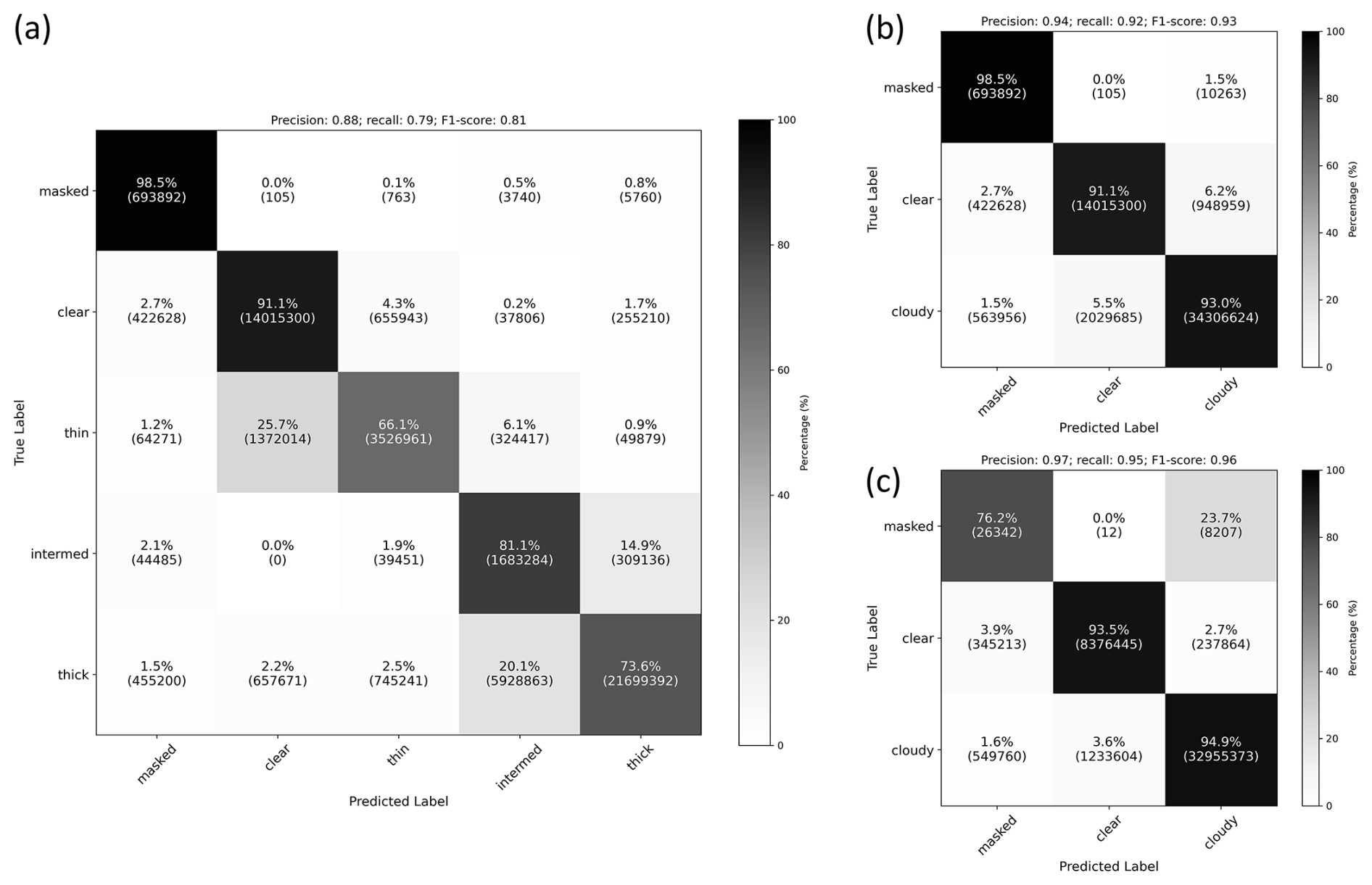
Figure 4 Confusion matrices of the segmentation algorithm output against the testing dataset. (a) Using all segmentation algorithm classes; (b) merging all cloudy classes to focus on cloudy-clear separation; and (c) same, but excluding testing samples with SZA exceeding 80°. The weighted precision, recall, and F1-score metrics for each testing subset are given in panel titles.

When assessing the testing dataset using such an approach, the algorithm's robustness is further demonstrated (Fig. 4b). In this case, only 6.2 % of the clear pixels and 5.5 % of the cloudy pixels are classified incorrectly. When we exclude from the evaluated pixels of the testing dataset scenes with SZA > 80°, which are challenging to all algorithms we are aware of (for reference, the TSI product does not provide output beyond an SZA of 87°), we see even more robust results with merely 2.7 % of the clear pixels and 3.6 % of the cloudy pixels being classified incorrectly (Fig. 4c). These results are equivalent or superior to other cloud cover segmentation studies implementing ML algorithms such as CNN and transformers (cf. Dematties et al., 2023; Fa et al., 2019; Xie et al., 2020), especially when considering the evaluation of an extensive and fully independent testing data that includes sites not used in the training process. Note that the smaller correctly “masked” pixels in this case are the result of the exclusion of the bird image (Fig. 3b), taken when the solar disk was just above the horizon. With only a few bugs and some dirt left on the residual testing dataset, and the tendency to suggest a cloud “halo” around artifacts, we received this lower percentage. However, most of those incorrectly classified pixels are treated as “uncertain” and therefore should primarily be excluded from the cloud fraction calculations.

2.3 Segmentation Post-Processing

Following the segmentation algorithm operation, cloud cover is calculated by weighting each pixel by the effective sky area it represents in the observer's (camera) frame of reference. Following Long et al. (2006), this calculation is done using:

$$\begin{array}{}\text{(3)}& f={\displaystyle \frac{\sum l_i{N}_i^{\mathrm{cld}}}{\sum l_i{N}_i^{\mathrm{valid}}}},\end{array}$$

where f is the cloud fraction, $N_i^{\mathrm{cld}}$ and $N_i^{\mathrm{valid}}$ denote the number of valid cloudy and all valid pixels, respectively, and l_i is the pixel area correction factor calculated as:

$$\begin{array}{}\text{(4)}& l_i={\displaystyle \frac{\mathrm{2}\left(\cos {\mathit{\theta }}_{i\mathrm{1}}-\cos {\mathit{\theta }}_{i\mathrm{2}}\right)}{\left({\mathit{\theta }}_{i\mathrm{1}}^{\mathrm{2}}-{\mathit{\theta }}_{i\mathrm{2}}^{\mathrm{2}}\right)}},\end{array}$$

where θ_i1 and θ_i2 are the pixel zenith angles (in radians) at the edges of a given pixel i along the radial direction from the effective image center. Here, valid pixels are pixels within the 80° off-zenith effective FOV, not masked by site or solar disk masks (see Sect. 2.1), not classified as “masked” by the segmentation algorithm, and not considered uncertain.

Finally, in addition to the cloud cover in the full 80° FOV, ASISKYCOVER provides cloud cover estimates for a narrow FOV, in a region covering up to 5° off-zenith (e.g., the white circles in the right panels of Fig. 3).

2.4 Solar Disk State Classification Algorithm

In addition to the segmentation algorithm, we have trained a simplified binary random forest (RF) model to determine the solar disk state, which supplements the ASISKYCOVER product, with the possible solar disk state classes being “sun blocked” (by clouds) and “solar disk seen”. Note that we do not further partition the state classes to “solar disk seen through clear sky”, “solar disk seen through thin or intermediate-thick clouds”, and “partial solar disk blockage by clouds”. Classification of these solar states would require the trained model to be spatially-informed, suggesting that a convolutional neural network architecture should be used for a task of this type. Future updates to the ASISKYCOVER product could include such a more comprehensive solar disk state classification component.

The current RF solar disk state classification model is trained using the Scikit-Learn package (Pedregosa et al., 2011) and implements a set of features characterizing the brightness of pixels surrounding the solar disk center using only the red and blue channels. Those features are the minimum, maximum, mean, standard deviation, interdecile range, and the 5th, 10th, 25th, 50th, 75th, 90th, and 95th percentiles of pixels within circles with radii of 15, 25, and 50 pixels centered at the location of the solar disk center on training images (799 samples); the same manually labeled solar disk-designated images used to characterize the solar disk misalignment (Sect. 2.1).

Evaluation of the binary classification using an independent testing dataset consisting of 258 samples (roughly 75–25 train-test split) suggests robust performance of this classification model (Fig. 5) with all “solar disk seen” samples and 87 % of “sun blocked” samples being classified correctly. Model robustness is further indicated by an F1-score, precision, and recall values of 0.973, 0.947, and 1.000, respectively.

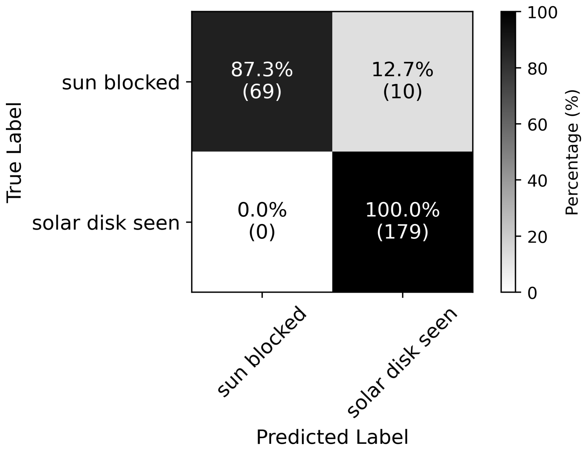
Figure 5 Confusion matrix of the solar disk state classification algorithm output against the testing data.

3 Results

3.1 Single-day time series

Figure 6 illustrates a time series of the ASISKYCOVER cloud cover data for 1 January 2024, at the SGP central site, demonstrating some of the information provided by this data product. As indicated by the top panel, representing the full FOV, cloud coverage exhibits a highly variable pattern prior to sunrise, followed by a steady and sharp rise to overcast conditions commensurate with sunrise. During this sharp cloud cover increase, clouds are initially classified as “thin”, but then quickly transition to thick-dominated clouds. The overcast conditions persist until after 19:00 UTC, when cloud type transitions back to thin-dominated, with several local bursts of cloud occurrence. The light pink curve, denoting the TSI sky cover product, describes a similar story with cloud cover largely staying within the ASISKYCOVER uncertainty range. However, the cloud onset occurs only after sunrise with a distinct offset relative to the ASISKYCOVER. In addition, the TSI cloud cover appears significantly underpredicted relative to ASISKYCOVER after 22:00 UTC, ∼1 h before sunset. Examination of the solar disk state classification output (pink markers) indicates that indeed the solar disk is visible after 19:00 UTC but is generally blocked by clouds before that, insinuating the possibility that the “intermediate” class fraction could be overestimated in this case to a certain extent, i.e., classified as “intermediate” instead of “thick”. Similarly, right after sunrise, it is likely that the thin-dominated period is misclassified, given that the solar disk state is classified as “blocked by clouds”, i.e., the low-light conditions render “thick” (or “intermediate”) clouds appear as the “thin” class. Examination of the inset ASI snapshots supports this general interpretation of the depicted time series although using other ARM datasets (as shown below) is needed to confirm the occurrence of intermediate and/or thick clouds around sunrise. (Note the challenge in even manually interpreting the 14:00 UTC snapshot taken shortly after sunrise; based on that snapshot, is it clear or cloudy?)

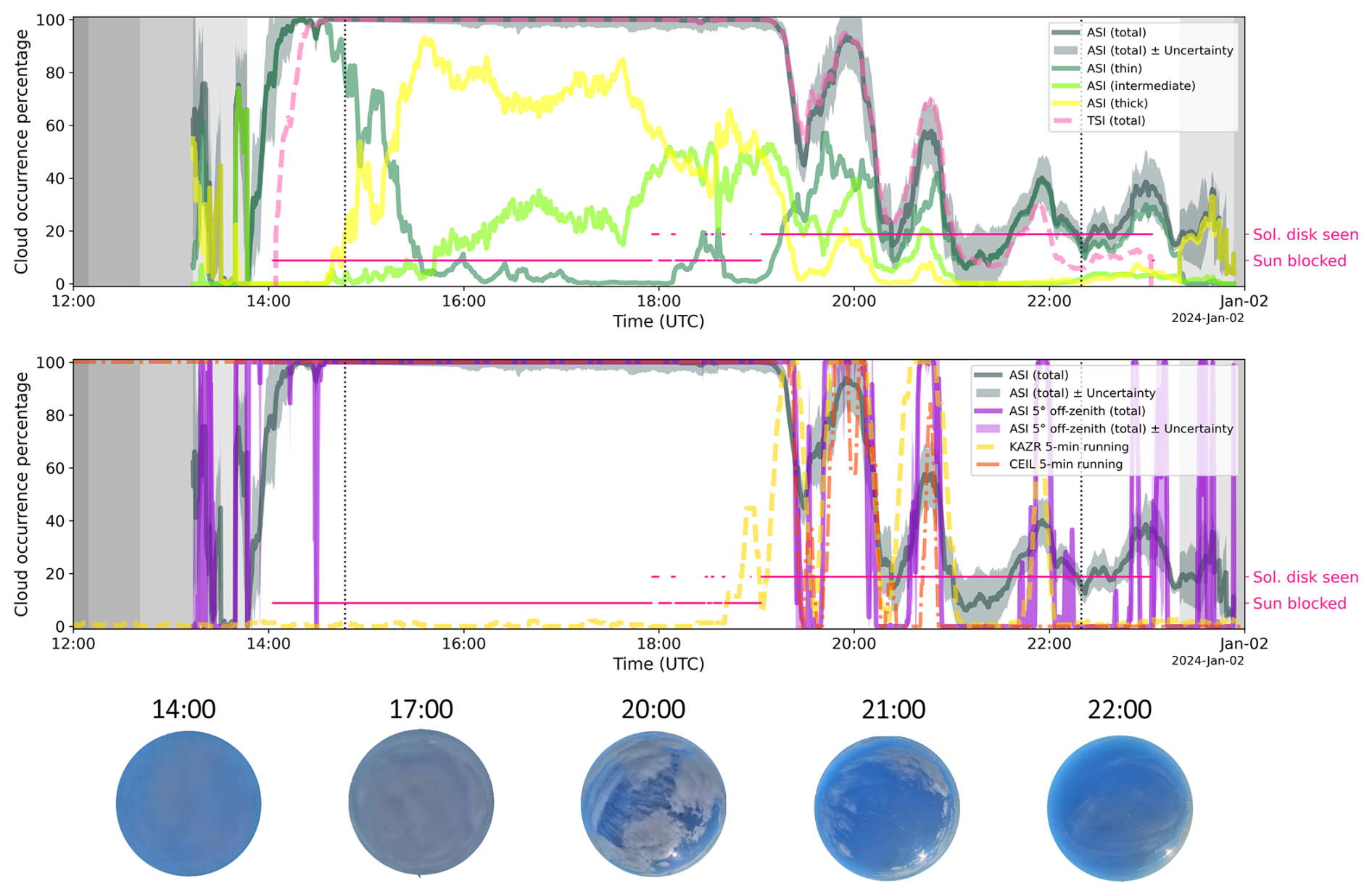
Figure 6 ASISKYCOVER cloud cover time series for the SGP central facility on 1 January 2024. (Top) Total cloud cover time series using the full 80° off-zenith field-of-view together with time series for the three cloud classes (see legend). The light pink curve illustrates the TSI sky cover time series. The pink markers denote the solar disk state classification output (see right y-axis labels). The grey-shaded regions extending until nearly 14:00 UTC and from roughly 23:00 UTC designate (in decreasing brightness) the civil twilight, nautical twilight, astronomical twilight, and nighttime. The vertical dotted black lines denote 80° SZA crosspoints. (Bottom) Similar, but showing the near-zenith (5° off-zenith) product time series together with the 5 min running mean Ka-band ARM Zenith Radar (KAZR; using moderate sensitivity mode echoes above 4 km range) and ceilometer cloud occurrence (see legend). A selected set of raw ASI images are shown at the bottom of the figure together with their corresponding times. (Note that the ASI images appear mirrored in the east-west direction; see Sect. 2.1 for details.)

To supplement the evaluation of the time series output, Ka-band ARM Zenith Radar (KAZR; Widener et al., 2012) and ARM ceilometer (CEIL; Morris, 2016) cloud occurrence time series data are illustrated in the bottom panel of Fig. 6 together with the near-zenith output of ASISKYCOVER. The KAZR and CEIL cloud occurrence percentages are averaged in 5 min running mean windows to mitigate their temporal point measurement operation difference from the spatial nature of the ASI. CEIL cloud occurrence instances are determined when the instrument indicates the occurrence of at least one cloud base height. KAZR-determined cloud instances are sample times with one or more moderate sensitivity (MD) mode echoes with signal-to-noise ratio exceeding −16 dB (see Silber et al., 2018) at radar range gates greater than 4 km. This dual instrument depiction accounts for the maximum CEIL (Vaisala CL31 model) range of 7 km, the lack of its cloud base height sensitivity to ice clouds, and the commonly occurring SGP KAZR echoes generated by biota at ranges of up to a few kilometers (below the freezing level). This multi-instrument depiction also streamlines figure interpretation. As such, the continuing CEIL cloud occurrence of 100 % preceding sunrise, commensurate with 0 % KAZR occurrence, suggests the occurrence of low-level clouds, and that the ASISKYCOVER cloud cover is significantly underpredicted before sunrise. In comparison, the TSI's 0 % cloud cover is a starker artifact. These challenging lighting conditions provide the main incentive for flagging ASISKYCOVER data at SZA values exceeding 80° (vertical dotted black lines in Fig. 6). That said, Fig. 6 suggests that clouds are intermittently indicated by the classification algorithm during the civil twilight. As shown from times later on the depicted day (after 18:30 UTC), the continuous CEIL-based cloud cover diminishes while the KAZR-based cloud cover increases in transient bursts, suggesting high cloud (cirrus) occurrence, consistent with the ASISKYCOVER analysis. However, while the change in total cloud cover is gradual in the ASISKYCOVER output, changes are more abrupt in the CEIL and KAZR time series data. The near-zenith product output displayed in the bottom panel of Fig. 6 resembles this abrupt change in cloud occurrence and further shows a general agreement between ASISKYCOVER and the CEIL and KAZR instruments (e.g., between 18:00 and 22:00 UTC).

3.2 Full-Year Analysis

Using the full year of processed ASISKYCOVER data, cloud cover over the SGP central site can be characterized for daytime conditions. Here, we exclude samples corresponding to SZA values exceeding 90°, which are considered less accurate (see previous section). ASISKYCOVER suggests a cloud cover of 56 % over the course of 2024, in agreement with the climatological results of Wang and Zhao (2017) for the SGP site based on the ARM Active Remote Sensing of Clouds (ARSCL; Clothiaux et al., 2001) dataset. Forty-nine percent of this annual cloud cover is classified as thin clouds. Assuming interchangeability between cloud thickness in this study and cloud altitude in other studies, this result is in qualitative agreement with previous climatologies for the SGP site (cf. Dong et al., 2006, their Fig. 1; Mace and Benson, 2008, their Fig. 4).

A 31 d running mean cloud cover evolution throughout the year is depicted in Fig. 7. Cloud cover at the beginning of the year fluctuates around 55 % in early January, with roughly equal contributions of thin and thick clouds. It then gradually increases until March, with the most prevalent classified cloud type being thick clouds until early February. From here through the end of the year, the thin cloud class is the most prevalent, though for the most part, its contribution to the total cloud cover is still smaller than the combination of the intermediate-thick and thick cloud types. The apparent thin cloud cover first peaks in early March with a 31 d mean cover of ∼38 % around the time when the total cloud cover has a global maximum (31 d mean of 73 % at a period centered on 13 March). Total cloud cover trends downwards starting in mid-March and stabilizes around 60 % between April and early July. It then gradually increases until late July, peaking at 68 %, commensurate with the global thin cloud cover peak of 42 %. From that point, total cloud cover generally trends downwards until mid-October, when thin clouds contribute close to 90 % of cloud cover over 31 d centered on 11 October, when the 31 d total cloud cover has a local minimum of 33 %. The total cloud cover continues to fluctuate around 40 % through early December, with the global 31 d mean total cloud cover minimum of 31 % in a window centered on 22 November. Finally, from early December, total cloud cover trends towards 50 % with an increasing prevalence of thick clouds, in what appears to be a setup for a repetition of early 2024 trends. Assuming interchangeability between cloud thickness and altitude (similar to the examples in Table 2), we observe qualitative agreement with climatological analyses of annual cloudiness and cloud-type variability over the SGP site (cf. Dong et al., 2006; Mace and Benson, 2008). However, additional analysis using other instrument datasets beyond the scope of this work is required to evaluate the influence of only using SGP daytime data (SZA < 90°) and its dependence on cloud type (e.g., Dong et al., 2005; Zhao et al., 2017), as well as to deconfound the influence of occluding cloud layers on the apparent occurrence of different cloud types.

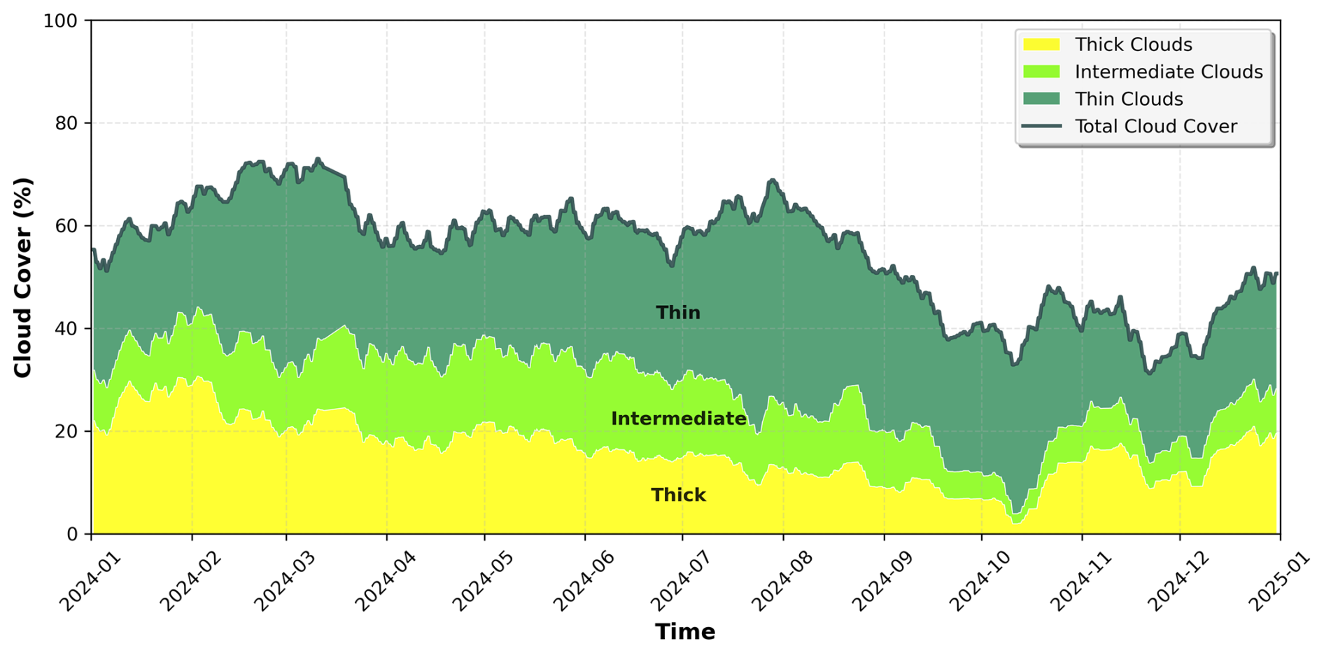
Figure 7 Cloud cover 31 d running-mean time series for the SGP site as determined by ASISKYCOVER for 2024. The stacked colored areas represent the distribution of cloud types (see legend and labels).

3.3 Bulk Comparison to Other ARM Datasets

Without a clear cloud cover benchmark, we begin this bulk comparison to the TSI product, the output dataset of which is the only direct equivalent to the ASISKYCOVER dataset. As suggested by the single-day time series presented in Fig. 6, ASISKYCOVER is generally consistent with the TSI product. However, the two products tend to have larger deviations and inconsistencies under certain conditions than others.

Figure 8 shows kernel density estimations (KDEs) of the ASISKYCOVER cloud cover deviations from the TSI cloud cover data product using the SGP central site 2024 data, conditioned on different variables. The interpretation of the depicted KDEs is based on numerous observed ASISKYCOVER and TSI scenes, which were qualitatively evaluated using expert judgment. On average, ASISKYCOVER exhibits a slightly higher tendency to detect more clouds than the TSI (by less than one percentage point) (Fig. 8a). However, the dataset difference variability is quite extensive, exceeding 14 percentage points.

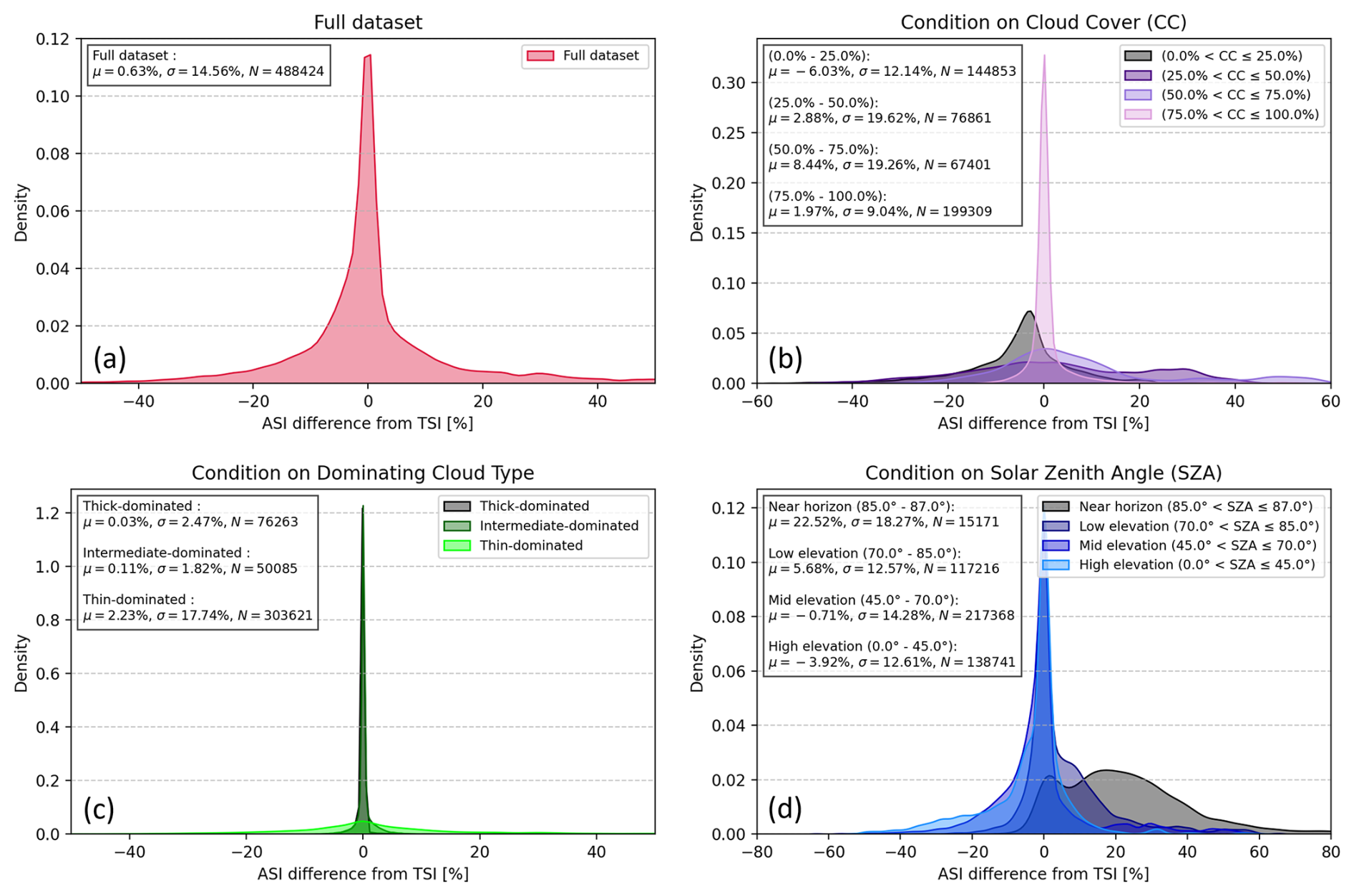
Figure 8 ASISKYCOVER deviations from the TSI cloud cover product kernel density estimations (KDEs) for SGP in 2024 while conditioning on different variables: (a) Full dataset (no conditioning), (b) ASISKYCOVER cloud cover (CC), (c) dominating cloud type per scene with CC greater than 5 % based on ASISKYCOVER, and (d) SZA (see legend). Mean deviation (μ), standard deviation (σ), and number of TSI-ASISKYCOVER sample pairs in the conditioned data subset (N) are given on the top left of each panel.

Examination of deviations while conditioning on the ASISKYCOVER total cloud cover (Fig. 8b) suggests that the TSI tends to detect a cloud cover that is ∼6 % higher in cases of clear to low cloud cover (up to 25 % based on ASISKYCOVER). In these cases, the TSI processing often incorrectly classifies clear pixels as cloudy, primarily due to solar flaring and resultant saturation of large image sectors. However, in broken cloud scenarios, there are cases in which the ASKISKYCOVER incorrectly classifies a cloudy pixel as clear. In those cases, the pixels are often flagged as uncertain, an ASISKYCOVER feature that is not reflected in this comparison. Scenes with extensive cloud cover (75 % up to overcast) are characterized by better agreement between the two data products, with relatively minor variability shown by the narrow KDE and a small standard deviation (SD) of ∼9 %. Such scenes are relatively more straightforward to classify, given that the most challenging image regions to classify are typically located at cloud edges. Vice versa, in relatively complex scenes with a mixture of cloudy and clear pixels, the product disagreement reaches its maximum with SD at ∼19 %.

The occurrence of thick clouds often characterizes overcast conditions over the SGP. Conditioning on the dominating (most prevalent per scene) cloud class (Fig. 8c), it is indicated that both data products have good agreement, with thick-dominated scene deviations smaller than 0.05 % on average and an SD of merely a few percent. The instrument cross-agreement is even better for scenes with intermediately thick cloud dominance, where the SD is smaller than 2 %. (We note that the TSI data product exhibits a very strong general tendency to classify clouds as “opaque” regardless of their true cloud thickness, and hence, to also underestimate the occurrence of thin clouds; not shown.) Figure 8c provides a clear indication of the challenge in consistently classifying thin cloud pixels (see Fig. 4). While on average, ASISKYCOVER detects total cloud cover higher by 1 percentage point in thin-cloud dominated scenes, the variability is distinctively higher (see KDEs), with SD on the order of 18 %. Those clear KDE patterns when partitioning based on dominating cloud type insinuate that the dominating cloud type per scene might be the best predictor for cloud detection algorithm consistency, and corroborate the class-dependent algorithm performance test results (Fig. 4).

Conditioning on SZA (Fig. 8d), product deviation variability remains large in all of the four examined ranges, but the average deviation provides additional information on instrument tendencies (note that the highest SZA is set to 87°, the maximum SZA value for which the TSI classification algorithm is applied). At high solar elevation (SZAs smaller than 45°), the TSI tends to overestimate the total cloud cover by ∼4 percentage points. This overestimation is primarily driven by very strong solar flaring saturating a large number of pixels, rendering them classified as cloudy. We note that the ASI at SGP suffers as well from solar flaring effects, though to a lesser extent than the TSI. However, our evaluation (not shown) suggests that ASI flaring effects are often starting to show during clear-sky scenes in the near-zenith pixels, and hence, the near-zenith product at SZA < 60°, which could be mitigated, to some extent, by using it in a quasi-binary approach as demonstrated below. At mid solar elevation (SZA between 45 and 70°), ASISKYCOVER and the TSI have reasonable agreement, with an average deviation of roughly half a percentage point. However, at higher SZAs, the ASI tends to suffer more from solar effects in the form of internal reflections, which are enhanced when the ASI has dirt on its housing, resulting in ASISKYCOVER overestimation (∼6 percentage points more classified cloudy pixels relative to the TSI in SZA between 70 and 85°). When the solar disk is near the horizon, however, ASISKYCOVER indicates total cloud cover that is higher by more than 20 percentage points relative to the TSI, which we attribute primarily to a loss of TSI sensitivity rather than ASI-related artifacts.

While this analysis points to some instrument and algorithm weaknesses, the limited conditioned variable ranges and lack of consideration of classification uncertainty, which the ASISKYCOVER data product provides, result in an incomplete picture regarding the ASISKYCOVER product evaluation. To perform a robust comparison to other ARM datasets, we examine the total cloud cover as a function of SZA – a variable independent of ASISKYCOVER output. Unlike a simple long-term time series analysis, for example, this approach deconvolves the changing length of day influence on the determined cloud cover, and facilitates the identification of instrument biases and tendencies, which were suggested in Fig. 8. We compare the ASISKYCOVER total cloud cover to the TSI sky cover data and the combination of the 5 min running mean KAZR and CEIL data described above (see Sect. 3.1). We acknowledge that the KAZR-CEIL combination is treated here as insensitive to SZA for all practical purposes and therefore assumed as unbiased on a first order basis, noting that most solar effects are typically detected when compared against nighttime data, which are excluded from this analysis. We also recognize that because of the field-of-view differences from the ASISKYCOVER, the KAZR-CEIL combination does not represent fully equivalent quantities even when the ASISKYCOVER near-zenith (NZ) product and 5 min running means are used. Therefore, the following comparison should primarily be treated as a consistency assessment rather than validation against a benchmark measurement.

Figure 9 shows the 2024 SGP central site ASISKYCOVER-determined cloud cover occurrence histogram as a function of SZA normalized for each SZA bin, together with mean cloud cover curves as a function of SZA for the ASISKYCOVER output, its NZ product, the TSI, and the KAZR-CEIL combination (see legend). Here, the NZ product is processed using a quasi-binary approach equivalent to the CEIL and KAZR point (i.e., non-spatial) measurement nature. To determine NZ cloud occurrence on a given scene (i.e., a value of 1), we require at least 99 % of the ∼5400 pixels within 5° off-zenith to be classified as one of the cloud classes (value set to 0 otherwise). The resultant binary time series is then used to calculate the 5 min running means. The 99 % threshold mitigates the low SZA solar flaring effects discussed above, at the limited expense of some under-estimation in scenes with partial cloud cover within the small 5° off-zenith region. The histogram at the bottom of Fig. 9 indicates that the ASISKYCOVER total cloud cover distribution is generally bi-modal regardless of SZA, with peaks at the distribution edges, i.e., clear (0 %–4 % cover) and overcast (96 %–100 % cover) conditions (see the darker histogram bins at the top and bottom of the depicted data). However, the clear conditions peak (histogram bottom) is much weaker and occasionally absent in specific SZA ranges.

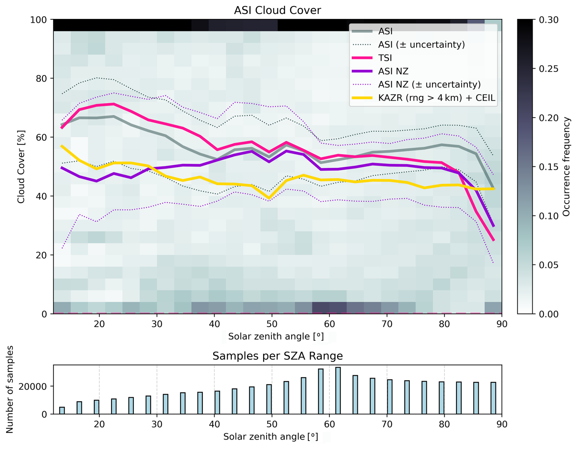
Figure 9 (Top) ASISKYCOVER-determined cloud cover occurrence frequency histogram as a function of SZA (bin sizes of 4 % and 3°, respectively) normalized for each SZA bin (i.e., each column of histogram bins sums to 1) for SGP in 2024. The mean cloud cover as a function of SZA is illustrated by the grey curve, with the dotted grey curves designating the mean ± sample uncertainties. The pink and yellow curves designate the mean cloud cover as a function of SZA for the TSI and the 5 min running average combination of ceilometer cloud base detections and KAZR moderate sensitivity (MD) mode echoes above 4 km, respectively (see Sect. 3.1). The purple solid and dotted curves represent the 5 min running average mean and mean ± sample uncertainty cloud cover as a function of SZA determined using the ASISKYCOVER near-zenith product (NZ; see text), rendering a more equivalent comparison to the KAZR-CEIL data. (Bottom) The total number of samples (images) per SZA bin range.

Consistent with KDE analysis above, the reduced peak at SZAs smaller than 36° is the result of solar flaring effects, resulting in sporadic higher cloud cover counts. These sporadic counts contribute to the increasing total cloud cover with a decreasing SZA pattern delineated by the mean ASISKYCOVER curve (grey). The TSI-determined cloud cover (pink) exhibits a similar trend, though with more pronounced overestimation. While one could suggest that this gradual enhancement is a mere artifact, the KAZR-CEIL curve (yellow) shows a similar behavior, which suggests cloud cover enhancement around local noon. Moreover, the cloud cover anti-correlation with SZA was not detected in an equivalent 1-year bulk analysis we performed of ASISKYCOVER output for the ARM ENA site (not shown).

Here, the ASISKYCOVER and TSI mean-cloud cover patterns appear to follow each other up to 60°, also consistent with the KAZR-CEIL patterns. From this SZA to roughly 80°, the ASISKYCOVER total cloud cover gradually increases, exceeding the TSI value, yet with the TSI remaining within the ASISKYCOVER uncertainty range (dotted grey curve). As indicated in the analysis above, this gradual increase results from the incorrect classification of clear pixels as cloudy, principally due to the combination of ASI housing dirt and internal reflection. In those cases, pixels are mostly classified as thin clouds, which explains the ASKISKYCOVER overestimation in low cloud cover scenes (Fig. 8b) and part of the variability in thin-dominated scenes (Fig. 8c) While these optical effects are observed throughout given ASI images, they are most pronounced close to the solar disk; at these SZA ranges, around the side of the image. Evidently, the NZ product (purple curve in Fig. 9) does not display this bogus gradual increase. Moreover, the equivalent ENA analysis (not shown) did not indicate any such artificial patterns, suggesting that this artifact tendency could be driven by local conditions (pollution, etc.) and influenced by the specific ASI instrument deployed at SGP. Above 80°, both the ASISKYCOVER and TSI products lose their cloud detection capability, though the ASISKYCOVER does so in a much weaker fashion, while retaining quantitative bulk agreement with the KAZR-CEIL combination. This agreement with the KAZR-CEIL is largely seen throughout all SZA ranges when accounting for the uncertainty ranges, in both the full FOV and NZ products. Furthermore, the mean curve pattern similarities tentatively suggest that ASISKYCOVER could be combined with zenith-pointing instruments for certain applications. We note that this full-FOV correspondence with point-measurement datasets might be somewhat different, depending on the prevailing cloud types (see Riley et al., 2020; Wagner and Kleiss, 2016).

4 Conclusions and Outlook

The ASISKYCOVER data product provides a thorough and comprehensive solution to the cloud cover determination challenge using all-sky imagers. It mitigates the influence of various artifacts such as bugs and dirt, and handles a wide range of scenarios. While still suffering some artifacts, especially when classifying scenes dominated by thin clouds and/or cases at high SZA, those artifacts are ameliorated by the ML-driven algorithm and are generally accounted for in the data product's uncertainty estimates. The algorithm is theoretically transferable to other all-sky imager platforms, likely with a new set of training data to address the different sensitivities, color saturation level and gain configurations, and resilience to pixel saturation and “solar flaring” in other image sensors.

ASISKYCOVER datasets are already being routinely generated for active and past ARM deployments involving the ASI instrument, and are available via the ARM Data Discovery. This data product will serve as the basis for ARM value-added data products (VAPs) that could include spatial classification and cloud height and movement tracking datasets handling multiple instruments and consecutive images, advanced artifact filtering by considerations of fixed objects in consecutive images, and more. Future development of the ASISKYCOVER algorithm will include spatially feature-based solar disk state classification (e.g., using convolutional neural networks), which will facilitate robust separation between conditions such as partial solar disk blocking by clouds and the distinction between the solar disk visibility through thin clouds or cloud-free air, as well as dedicated configurations for highly polluted sites and events. As demonstrated here, the introduction of ASISKYCOVER ensures the continuation of the long-term cloud cover records ARM collected using the TSI, while the various features of ASISKYCOVER open new avenues for future developments and dataset enhancements.