Configuration of climatological limits for surface radiation measurement quality control: a global assessment using a novel radiation climate classification

Quality control (QC) of ground-based solar radiation measurements is fundamental to ensuring the integrity of surface energy balance and climatological studies. The extremely rare limit (ERL) test, a widely implemented QC standard, is frequently noted for being overly conservative, often failing to isolate subtle instrumental or environmental anomalies. To improve QC tightness and sensitivity, this study presents a data-driven framework for configuring regime-specific climatological limits. Diverging from traditional climate classifications that do not directly account for radiative variability, we define seven distinct radiation regimes through unsupervised learning, utilizing principal component analysis and hierarchical clustering. For each identified regime, optimal test coefficients are established via a machine-learning-based optimization strategy. Specifically, we maximize the F₁ score by benchmarking the climatological limit test against an isolation forest outlier detection model. Validation using global measurements from the Baseline Surface Radiation Network demonstrates that the proposed regional limits provide a significantly tighter fit to observed data distributions compared to the original global ERL thresholds. This methodology offers a scalable and automated approach to regionalizing QC procedures, substantially enhancing the precision of global radiation monitoring networks.

1 Introduction

Surface solar radiation is an important variable in both atmospheric science and solar energy engineering (Yang and Kleissl, 2024). Radiation information is commonly obtained from three sources: ground-based measurements, satellite remote sensing, and numerical modeling (Yang et al., 2022). Among these options, ground-based measurements provide the highest accuracy and are therefore widely used to evaluate gridded products (Wandji Nyamsi et al., 2023; Elias et al., 2024) and to provide training targets for radiation models (Wiltink et al., 2025; Song et al., 2025). However, because of instrument maintenance, malfunction, degradation, and other operational issues, ground-based measurements cannot be assumed to be error-free and must be quality-controlled. Consequently, substantial effort has been devoted to developing quality control (QC) methods and routines for surface radiation measurements (Forstinger et al., 2021). In this context, the core task is one of outlier detection, in which samples are classified as inliers or outliers, often referred to as “good” and “bad” samples.

Outlier detection has deep roots in statistics. One of the most basic methods is the boxplot introduced by Tukey (1975), in which points located more than 1.5 interquartile ranges beyond the box are flagged as anomalies. Many boxplot variants have since been proposed for more complex settings, including letter-value plots for large datasets (Hofmann et al., 2017) and bagplots for bivariate datasets (Rousseeuw et al., 1999). Beyond boxplot-type approaches, statistical outlier detection methods are commonly categorized as density-, distance-, or cluster-based; the reader is referred to Smiti (2020) for a review. Density-based methods assume that anomalies occur in low-probability regions. Distance-based methods assume that anomalies lie far from neighboring observations. Cluster-based methods partition data into groups and identify anomalies as samples that do not fit any group. Regardless of method, effectiveness is maximized when domain knowledge is incorporated.

For surface radiation measurements, domain knowledge can be grouped into two categories: information related to the radiation quantities themselves and information related to instrumentation. For example, the widely used extremely rare limit (ERL) test proposed by Long and Dutton (2002) incorporates both categories by defining upper limits for shortwave radiation quantities as functions of the cosine of the solar zenith angle, with an additional constant term that accounts for measurement uncertainty. The ERL test is expressed as

$$\begin{array}{}\text{(1)}& {\displaystyle }-\mathrm{2}{\text{ W\hspace{0.17em}m}}^{-\mathrm{2}}& {\displaystyle }\le G_{\mathrm{h}}\le \mathrm{1.2}{E}_{\mathrm{0}n}{\mathit{\mu }}_{\mathrm{0}}^{\mathrm{1.2}}+\mathrm{50}{\text{ W\hspace{0.17em}m}}^{-\mathrm{2}},\text{(2)}& {\displaystyle }-\mathrm{2}{\text{ W\hspace{0.17em}m}}^{-\mathrm{2}}& {\displaystyle }\le B_{\mathrm{n}}\le \mathrm{0.95}{E}_{\mathrm{0}n}{\mathit{\mu }}_{\mathrm{0}}^{\mathrm{0.2}}+\mathrm{10}{\text{ W\hspace{0.17em}m}}^{-\mathrm{2}},\text{(3)}& {\displaystyle }-\mathrm{2}{\text{ W\hspace{0.17em}m}}^{-\mathrm{2}}& {\displaystyle }\le D_{\mathrm{h}}\le \mathrm{0.75}{E}_{\mathrm{0}n}{\mathit{\mu }}_{\mathrm{0}}^{\mathrm{1.2}}+\mathrm{30}{\text{ W\hspace{0.17em}m}}^{-\mathrm{2}},\end{array}$$

where G_h, B_n, and D_h denote the global horizontal irradiance (GHI), beam normal irradiance (BNI), and diffuse horizontal irradiance (DHI), respectively; μ₀=cos Z is cosine of the solar zenith angle; and E_0n is the extraterrestrial irradiance, computed using the solar constant (E_sc=1361.1 W m⁻²), the average sun–earth distance over the course of one revolution (R_avg), and the current sun–earth distance (R), see Yang et al. (2026):

$$\begin{array}{}\text{(4)}& {\displaystyle }{E}_{\mathrm{0}n}=E_{\text{sc}}{\left({\displaystyle \frac{R_{\text{avg}}}{R}}\right)}^{\mathrm{2}}.\end{array}$$

The ERL test is recommended by the Baseline Surface Radiation Network (BSRN) and is widely used in both climate and solar-energy applications (Driemel et al., 2018).

However, one key limitation of the ERL test in Eqs. (1)–(3) is that the limits are often too loose. Figure 1 shows one year (2024) of 1 min measurements from the BSRN Qiqihar (QIQ) station (Chen et al., 2025), together with the corresponding ERL values. The mismatch is clear: the ERL envelopes are overly conservative and therefore provide limited QC sensitivity. Consistent with Nollas et al. (2023), the ERL test typically rejects far fewer records than other QC tests, such as the three-component closure test. Therefore, the objective of this study is to derive improved ERL coefficients. This direction was already suggested by Long and Shi (2008), who recommended configurable climatological upper limits. Denoting the cosine of the solar zenith angle by μ₀, the configurable limits are written as

$$\begin{array}{}\text{(5)}& {\displaystyle }{G}_{\mathrm{h}}& {\displaystyle }\le a_G{E}_{\mathrm{0}n}{\mathit{\mu }}_{\mathrm{0}}^{b_G}+\mathrm{50}{\text{ W\hspace{0.17em}m}}^{-\mathrm{2}},& {\displaystyle }& {\displaystyle }\text{(6)}& {\displaystyle }{B}_{\mathrm{n}}& {\displaystyle }\le a_B{E}_{\mathrm{0}n}{\mathit{\mu }}_{\mathrm{0}}^{b_B}+\mathrm{10}{\text{ W\hspace{0.17em}m}}^{-\mathrm{2}},& {\displaystyle }& {\displaystyle }\text{(7)}& {\displaystyle }{D}_{\mathrm{h}}& {\displaystyle }\le a_D{E}_{\mathrm{0}n}{\mathit{\mu }}_{\mathrm{0}}^{b_D}+\mathrm{30}{\text{ W\hspace{0.17em}m}}^{-\mathrm{2}},& {\displaystyle }& {\displaystyle }\end{array}$$

where the six coefficients $a_G,b_G,\mathrm{\dots },b_D$ are to be determined using several years of climate-, region- or site-specific data. We note that, in principle, one can further configure the constant terms. Nevertheless, such practices may result in very low constant terms that can no longer represent the measurement uncertainty.

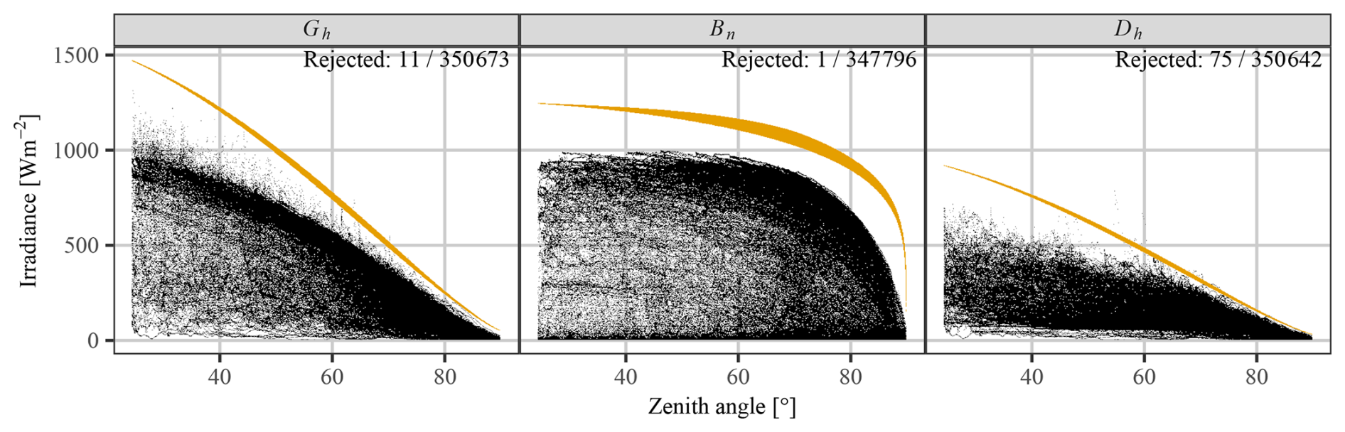
Figure 1 One year (2024) of 1 min irradiance measurements from the QIQ station (black) with their corresponding ERL values (orange). The ERL boundary limits appear as regions, rather than lines, due to the joint dependence of the ERL criterion on solar zenith angle and the seasonal variation of the sun–earth distance.

At this stage, two questions arise: (1) how many coefficient sets should be configured for global application, and (2) how should those coefficients be determined? The first question concerns clustering. The objective is to define radiation climatic regimes from global observations and then derive one coefficient set for each regime. A possible choice is the Köppen–Geiger climate classification (e.g., Beck et al., 2018); however, that framework is based primarily on temperature and precipitation and is therefore not specifically tailored to solar-radiation variability. There are also radiation-oriented classifications proposed (e.g., Yang et al., 2024a), but the procedures are often based on low-dimensional climatological variables such as annual cloud cover and aerosol loading. Accordingly, this study adopts a data-driven approach that groups high-resolution BSRN radiation measurements into seven radiation climatic regimes. Clustering is performed by combining principal component analysis (PCA) and hierarchical clustering. To avoid the computational burden associated with high-dimensional time-series inputs, where each timestamp is treated as a feature (Yang et al., 2017), clustering is conducted in a carefully designed feature space.

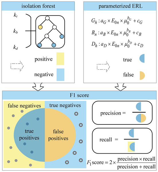
The second question concerns optimization. The objective is to determine coefficients using an explicit and reproducible criterion. The main challenge is that true anomalies are unknown during QC. In Long and Shi (2008), no specific method was provided for determining configurable coefficients. Yang et al. (2018) proposed gradually reducing coefficients until a sudden increase in rejection rate occurs; however, this strategy still involves subjective judgment. In binary classification, performance is commonly evaluated using the F₁ score, which is computed from a confusion matrix containing true positive (TP), true negative (TN), false positive (FP), and false negative (FN) counts. In this study, the confusion matrix is constructed from two inlier–outlier classifications: one from the climatological-limit test, i.e., Eqs. (5)–(7), and one from the isolation forest (iForest) method. Maximizing the F₁ score yields the highest agreement between the two QC classifications. This optimization is solved using the limited-memory Broyden–Fletcher–Goldfarb–Shanno algorithm with bounds (L-BFGS-B).

2 Data and method

2.1 BSRN data

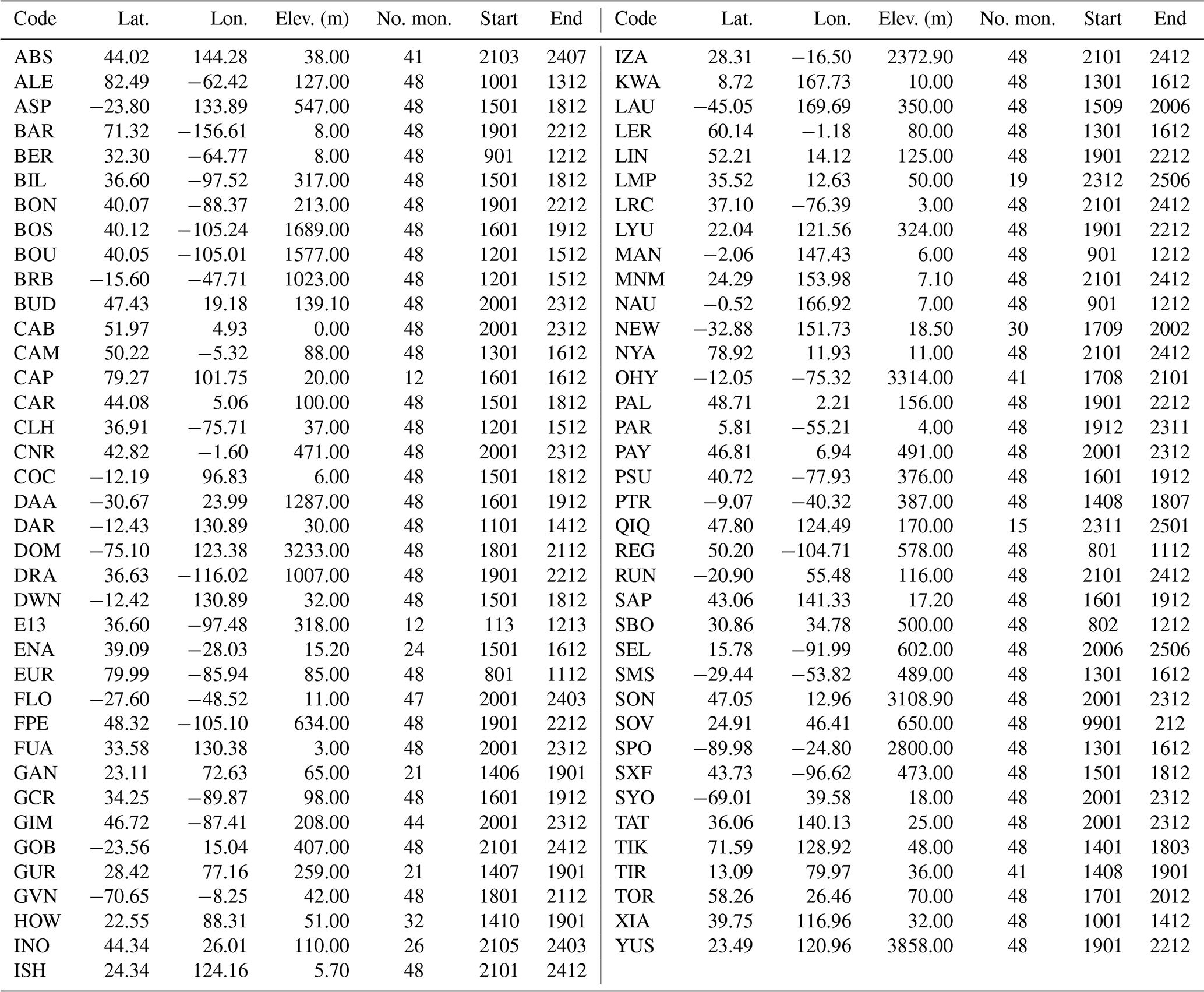
The data used in this study are from the Baseline Surface Radiation Network (BSRN), which is widely regarded as a reference-quality archive of ground-based radiation measurements (Driemel et al., 2018; Ohmura et al., 1998). The observations are available from the official BSRN FTP server and from PANGAEA, which is an open-access data publisher for earth and environmental science. This study uses shortwave radiation quantities (G_h, B_n, and D_h) from 75 stations, and the corresponding station metadata are listed in Table 1. These stations span all five continents and islands in all four oceans, providing broad coverage of global radiation regimes. To balance representativeness and data volume, the most recent continuous 4-year period is selected for each station. If a station does not meet this criterion, all available records are used.

Table 1 Metadata of the 75 BSRN stations used in this study. “Start” and “End” are reported in yymm format (year and month).

Because solar radiation quantities exhibit both annual and diurnal cycles, it is customary to use normalized indices (or k indices) in data analysis. There are multiple normalization options, and the simplest is to convert irradiances to transmittances. For G_h, B_n, and D_h, the corresponding transmittances (k_t, k_b, and k_d) are computed as follows:

$$\begin{array}{}\text{(8)}& {\displaystyle }{k}_{\mathrm{t}}& {\displaystyle }={\displaystyle \frac{G_{\mathrm{h}}}{E_{\mathrm{0}}}},& {\displaystyle }& {\displaystyle }\text{(9)}& {\displaystyle }{k}_{\mathrm{b}}& {\displaystyle }={\displaystyle \frac{B_{\mathrm{n}}}{E_{\mathrm{0}n}}},& {\displaystyle }& {\displaystyle }\text{(10)}& {\displaystyle }{k}_{\mathrm{d}}& {\displaystyle }={\displaystyle \frac{D_{\mathrm{h}}}{E_{\mathrm{0}}}},& {\displaystyle }& {\displaystyle }\end{array}$$

where E₀=E_0nμ₀ is the extraterrestrial GHI; the notation for the transmittances follows the widely accepted convention in solar energy meteorology (Shen et al., 2026; Ma and Yang, 2026). In many references, k_t is referred to as the clearness index (Yang et al., 2024b). Similar to the three radiation quantities, the transmittances also satisfy the closure relationship,

$$\begin{array}{}\text{(11)}& {\displaystyle }{k}_{\mathrm{t}}=k_{\mathrm{b}}+k_{\mathrm{d}}.\end{array}$$

In the clustering analysis below, the k_t, k_b, and k_d time series are used. Furthermore, all nighttime data points (defined here as Z>85°) are removed. In addition, a filter requiring k_t, k_b, and k_d to be greater than zero is applied to exclude low-sun observations, which often exhibit high noise because of radiometer design limitations (Liu et al., 2025).

2.2 Radiation climatological feature selection

In this study, radiation climatological features are selected to group sites with similar radiation regimes, so that QC coefficients can be developed at the group level rather than for individual sites. Defining radiation regimes has been attempted in numerous studies and is referred to as radiation zoning (Li et al., 2013) or radiation climate classification (Dash et al., 2017). In most studies, radiation regimes are defined by clustering monthly or daily mean radiation variables or the clearness index (e.g., de las Heras et al., 2026; Jiang et al., 2021; Anas et al., 2021). However, as data resolution increases, the clustering dimensionality – where each measurement can be treated as one dimension – quickly becomes computationally infeasible, even with dimension-reduction techniques. Therefore, this study uses radiation climatological features to represent high-resolution radiation data.

Three feature classes are considered: (1) zenith-angle range, (2) harmonic-analysis features, and (3) probability-density-function (PDF) features. The zenith-angle range is included because it is directly involved in QC (Eqs. 5–7), where climatological limits are configured as a function of Z. Intuitively, using the same QC envelope (cf. Fig. 1) for one site with a minimum zenith angle of 50° and another with a minimum zenith angle of 0° is inadequate. Harmonic analysis describes seasonal patterns (not limited to annual and diurnal cycles) in radiation time series, which are related to the range and shape of the scatter points in Fig. 1. Harmonic analysis has also long been used as a stand-alone tool for radiation climate classification (Terjung, 1970; Horn and Bryson, 1960). In addition, the PDFs of solar-radiation transmittances (k_t, k_b, and k_d) are known a priori to be tied to prevailing local sky conditions. For example, arid sites are expected to show higher probability concentrations in the high-k_t range. Thus, careful PDF analysis can extract statistical descriptors of radiation regimes. Because the zenith-angle range is straightforward to obtain, the extraction of the other two feature classes is described below.

2.2.1 Harmonic-based features

For a given time series {y_t}, with $t=\mathrm{1},\mathrm{\dots },T$, harmonic analysis assumes that the series can be decomposed into an infinite series of harmonic components (Jakubauskas et al., 2001). Mathematically, this is expressed as

$$\begin{array}{}\text{(12)}& {\displaystyle }{y}_t=c_{\mathrm{0}}+\sum _{n=\mathrm{1}}^{\mathrm{\infty }}{a}_n\cos {\displaystyle \frac{\mathrm{2}\mathit{\pi }nt}{T}}+\sum _{n=\mathrm{1}}^{\mathrm{\infty }}{b}_{\mathrm{n}}\sin {\displaystyle \frac{\mathrm{2}\mathit{\pi }nt}{T}}.\end{array}$$

By defining the jth harmonic as the jth term in the Fourier series, it follows that

$$\begin{array}{}\text{(13)}& {\displaystyle }{a}_j\cos {\displaystyle \frac{\mathrm{2}\mathit{\pi }jt}{T}}+b_j\sin {\displaystyle \frac{\mathrm{2}\mathit{\pi }jt}{T}}=c_j\cos \left({\displaystyle \frac{\mathrm{2}\mathit{\pi }jt}{T}}-{\mathit{\varphi }}_j\right),\end{array}$$

where $c_j=\sqrt{a_j^{\mathrm{2}}+b_j^{\mathrm{2}}}$ and ${\mathit{\varphi }}_j=\arctan (b_j/a_j)$ are known as the amplitude and phase angle of the jth harmonic. In practice, it is common to use a reduced form of Eq. (12) by neglecting the higher harmonics and including an error term:

$$\begin{array}{}\text{(14)}& \begin{array}{rl}{y}_t& =c_{\mathrm{0}}+\sum _{j=\mathrm{1}}^m{a}_j\cos {\displaystyle \frac{\mathrm{2}\mathit{\pi }jt}{T}}+\sum _{j=\mathrm{1}}^m{b}_j\sin {\displaystyle \frac{\mathrm{2}\mathit{\pi }jt}{T}}+{\mathit{\epsilon }}_t\\ & =c_{\mathrm{0}}+\sum _{j=\mathrm{1}}^m{c}_j\cos \left({\displaystyle \frac{\mathrm{2}\mathit{\pi }jt}{T}}-{\mathit{\varphi }}_j\right)+{\mathit{\epsilon }}_t.\end{array}\end{array}$$

Eq. (14) can be solved efficiently by least squares, yielding $(c_{\mathrm{0}},c_{\mathrm{1}},\mathrm{\dots },c_m,{\mathit{\varphi }}_{\mathrm{1}},\mathrm{\dots },{\mathit{\varphi }}_m)$, which can be used to construct the fitted line for any given t and T.

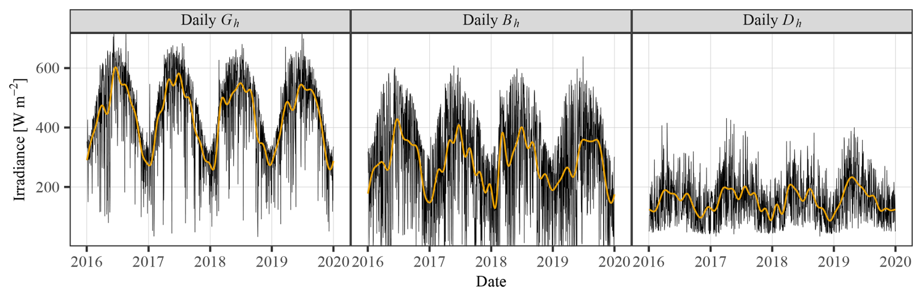
In this study, harmonic analysis is applied to daily G_h, B_n, and D_h time series. The number of harmonics (m) is empirically set to 25; the choice is made through an empirical sensitivity analysis aimed at balancing the goodness of the seasonal fit against the risk of overfitting. Figure 2 shows results for the Boulder station (BOS), United States, and demonstrates that seasonal variability in irradiance components is captured well. Two features are extracted for each of G_h, B_n, and D_h: (1) c₀, representing the irradiance level, i.e., the intercept, and (2) the range, i.e., the maximum minus minimum over all four years, of the harmonic regression fit, representing seasonal irradiance contrast. Thus, harmonic analysis provides six features in total. While adjusting the harmonic order may slightly alter specific feature values, the resulting changes remain small compared to the distinct differences observed between sites. Therefore, the impact on the final radiation climate classification is expected to be negligible.

Figure 2 Harmonic analysis of daily G_h, B_h, and D_h time series at the BOS station.

2.2.2 Density-based features

The density-based features are extracted from the transmittances, rather than from irradiance components themselves, because the latter random variables are “contaminated” by yearly and diurnal cycles and are thus unable to fully reflect sky conditions. There are numerous studies in the literature dealing with the statistical distribution of k_t, but far fewer on k_b and k_d. For instance, Jurado et al. (1995) proposed using a two-component normal mixture model for 5 min k_t, whereas Hollands and Suehrcke (2013) suggested a three-component normal mixture model for 1 min k_t. Regardless, a consensus in the literature is that transmittance distributions are rarely unimodal, because at least three groups of sky conditions generally exist: clear, cloudy, and overcast (Yagli et al., 2019; Lou et al., 2019). On this point, recent work by Shen et al. (2026) and Zhang et al. (2024) revealed that component distributions are often asymmetric, which justifies the use of skew-normal distributions during modeling.

A mixture model is simply the convex combination of several component distributions, that is,

$$\begin{array}{}\text{(15)}& {\displaystyle }g(x;\mathbf{\Theta }){\displaystyle }=\sum _{j=\mathrm{1}}^m{p}_j{f}_j(x;{\mathit{\theta }}_j),\text{s.t. }\sum _{j=\mathrm{1}}^m{p}_j=\mathrm{1}\end{array}$$

where g(⋅) is the PDF of a multi-modal random variable, f_j(⋅) is the PDF of jth component, Θ and θ_j are parameter vectors of the respective PDFs, where $\mathbf{\Theta }={\left(p_{\mathrm{1}},\mathrm{\dots },p_m,{\mathit{\theta }}_{\mathrm{1}}^{\top },\mathrm{\dots },{\mathit{\theta }}_m^{\top }\right)}^{\top }$. For instance, the PDF of a skew-normal distribution is

$$\begin{array}{}\text{(16)}& {\displaystyle }f(x;\mathit{\theta })={\displaystyle \frac{\mathrm{2}}{\mathit{\omega }}}\mathit{\varphi }\left({\displaystyle \frac{x-\mathit{\xi }}{\mathit{\omega }}}\right)\mathrm{\Phi }\left(\mathit{\alpha }{\displaystyle \frac{(x-\mathit{\xi })}{\mathit{\omega }}}\right),\end{array}$$

where $\mathit{\theta }=(\mathit{\xi },\mathit{\omega },\mathit{\alpha }{)}^{\top }$ is the parameter vector holding the location, scale, and shape parameters; ϕ(⋅) is the PDF of a normal distribution; and Φ(⋅) is the cumulative distribution function of the standard normal distribution. For a three-component skew-normal distribution,

$$\begin{array}{}\text{(17)}& {\displaystyle }\mathbf{\Theta }={\left(p_{\mathrm{1}},p_{\mathrm{2}},p_{\mathrm{3}},{\mathit{\xi }}_{\mathrm{1}},{\mathit{\omega }}_{\mathrm{1}},{\mathit{\alpha }}_{\mathrm{1}},{\mathit{\xi }}_{\mathrm{2}},{\mathit{\omega }}_{\mathrm{2}},{\mathit{\alpha }}_{\mathrm{2}},{\mathit{\xi }}_{\mathrm{3}},{\mathit{\omega }}_{\mathrm{3}},{\mathit{\alpha }}_{\mathrm{3}}\right)}^{\top },\end{array}$$

which can be estimated using a variety of methods, such as the method of moments (MOM) and maximum likelihood estimation (MLE). It is highlighted that fitting mixture distribution requires an initial condition. In this work, MOM is used for that purpose, and MLE follows.

With the above preliminaries, Fig. 3a depicts the estimated densities of three different mixture models, using k_t data from the BOS station. It can be seen that the three-component mixtures have a clear advantage over the two-component mixture. In terms of feature selection, the area under the left-most component PDF and the area under the right-most component PDF are considered, for they correspond to the probability of overcast and clear-sky conditions, respectively. It should be highlighted that the component PDFs are not necessarily ordered, and the left- and right-most PDFs need to be identified through computing the mean values. For a skew-normal distribution, its mean value is given by

$$\begin{array}{}\text{(18)}& {\displaystyle }\mathit{\xi }+\mathit{\omega }\mathit{\delta }\sqrt{{\displaystyle \frac{\mathrm{2}}{\mathit{\pi }}}},\text{ where }\mathit{\delta }={\displaystyle \frac{\mathit{\alpha }}{\sqrt{\mathrm{1}+{\mathit{\alpha }}^{\mathrm{2}}}}}.\end{array}$$

In other words, we first compute the mean values of f₁, f₂, and f₃, and then sort them from smallest to largest. After that, the p_j's that correspond to the smallest and largest mean values are selected as features.

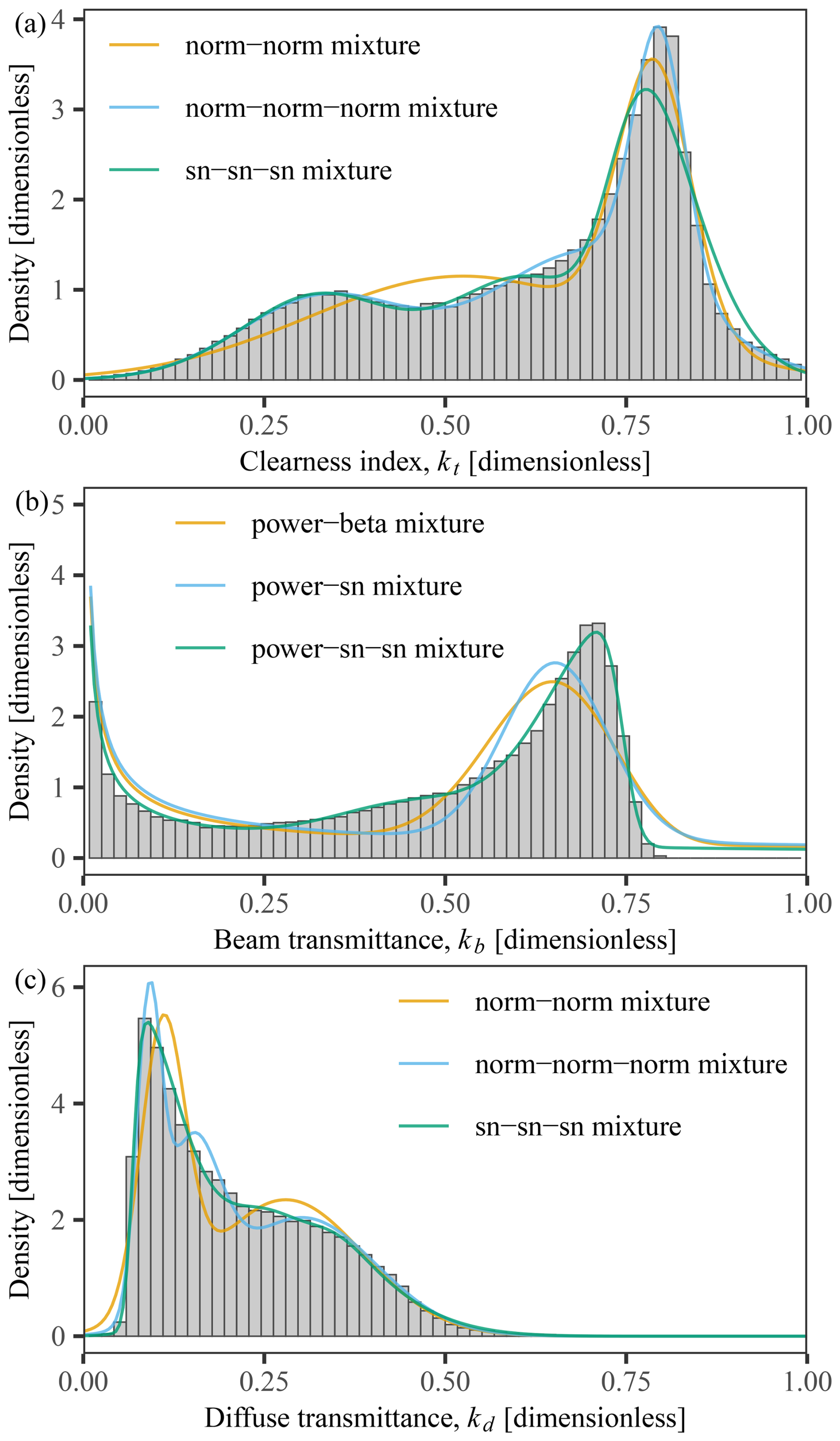
Figure 3 Histograms of k_t, k_b, and k_d at the BOS station, alongside density functions computed using selected mixture models. The short form “norm” and “sn” in the legend represent “normal” and “skew normal,” respectively.

As for k_d, its analysis is analogous to that of k_t. Specifically, a three-component skew-normal mixture model is compared against two- and three-component normal mixture models in Fig. 3c, showing evident superiority in explaining the distribution of k_d. Feature selection is also analogous, i.e., the areas under the left- and right-most component PDFs are retrieved. That said, the situation with k_b differs from that of the other two transmittances. More specifically, the value of B_n and thus k_b drops to near zero in the presence of clouds – this results in a sharp rise in probability at k_b=0, which cannot be modeled using normal distributions. Considering that the probability near k_b=0 gradually declines as k_b increases, there are many options for component distributions, including exponential, Weibull, gamma, and beta distributions, among others. Among the different options, the power distribution bounded on [0,1] is particularly useful for its simplicity and flexibility, and is therefore chosen. The PDF of a standard power distribution is:

$$\begin{array}{}\text{(19)}& {\displaystyle }f\left(x\right)=a{x}^{(a-\mathrm{1})},\end{array}$$

where a is the only parameter to be estimated. Using a power distribution as a basis, several mixture models are compared in Fig. 3b, and the option with one power distribution and two skew-normal distributions shows the best fit. Similar to the two former cases, the areas under the power distribution and the right-sided skew-normal distribution are selected as features.

It is noted in Fig. 3b that the observed density exceeding the theoretical boundaries of [0,1] and the fit near zero are consequences of the parametric model structure, specifically the unbounded support of the skew-normal components and the mathematical behavior of the power-law component, rather than the addition of an explicit linear constant. These minor fitting artifacts do not impact our results, as our analysis relies on the mixture weights to characterize site-specific radiation climates. Furthermore, our pre-filtering of k_b ensures that the maximum likelihood estimation is driven by the distribution's core (e.g., clear-sky vs. cloudy-sky modes) rather than its boundaries.

2.3 Dimension reduction and clustering

With the extracted radiation climatological features, the next step involves dimensionality reduction and clustering. This process ensures that stations from locations worldwide are allocated into sensible groups, allowing for the configuration of group-specific QC limits. In this work, we employ PCA followed by Ward's hierarchical clustering. This combination is chosen for its ability to handle feature redundancy while providing a structured, multi-level grouping of stations based on their variance profiles.

PCA transforms correlated variables into a new set of orthogonal principal components. These components are linear combinations of the original features, ordered by explained variance. To avoid errors in distance calculations during clustering, rows containing missing values are removed before analysis. Following standard practice, a 90 % variance-retention threshold is applied. In this implementation, the first seven principal components are retained because they jointly satisfy this threshold.

These seven principal components are then used as inputs to hierarchical clustering with Ward's minimum-variance criterion. Unlike k-means, which requires the number of clusters to be predefined, hierarchical clustering builds a nested tree structure (dendrogram) from Euclidean distances. To determine the optimal number of clusters (k), we conduct silhouette analysis for k=4 to 10. The final value of k is selected by maximizing the mean silhouette width, which balances high intra-cluster cohesion and strong inter-cluster separation. This procedure yields a cluster configuration that effectively categorizes stations by their geographic and climatological characteristics.

2.4 QC using climatological limits and iForest

To define radiation-regime-specific climatological limits for QC, two complementary outlier-detection methods are used: the ERL test and the iForest algorithm. Both methods produce binary outlier–inlier classifications, and their agreement is quantified using the F₁ score. Because the ERL parameters directly determine the QC outcome, they are configured by maximizing F₁. This maximization problem is solved with L-BFGS-B. In other words, the ERL parameter set that yields the highest F₁ score is adopted as the optimal climatological limit for each climate category. The detailed implementation is presented in the following sections, and the complete QC-configuration workflow is shown in Fig. 4.

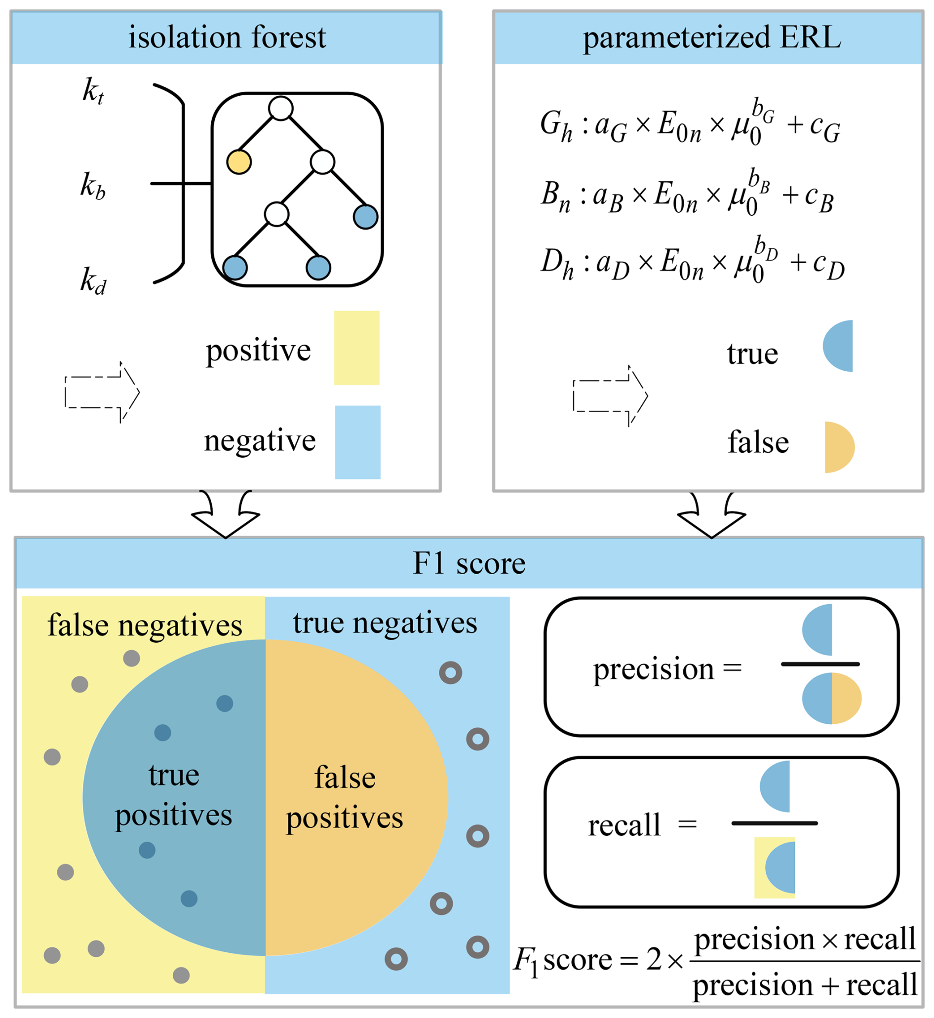
Figure 4 Workflow for configuring climatological QC limits. The procedure iteratively adjusts the parameters of two independent outlier detection algorithms to maximize the F₁ score derived from their agreement.

2.4.1 Climatological limits for true and false value determination

In the BSRN QC procedure, outliers are detected according to Eqs. (5)–(7). To establish stricter criteria for regime-specific QC evaluation, the test parameters are adjusted. Data points outside the QC limits are labeled false (F), whereas points within the acceptable range are labeled true (T). In other words, samples within the ERL limits are treated as likely valid observations, while samples exceeding the limits are treated as likely problematic observations.

2.4.2 Isolation forest for positive and negative value determination

The iForest algorithm is an unsupervised anomaly-detection method based on decision-tree principles. Its core concept is the isolation property of anomalies: anomalous points tend to lie far from the main point cloud or in regions with distinct density. Compared with conventional clustering methods, such as kernel density estimation (KDE) and Gaussian mixture models (GMM), iForest offers several practical advantages. Conventional clustering methods often rely on features such as solar zenith angle and irradiance; because these variables have different units, distance- or density-based approaches can perform unsatisfactorily. Similarly, KDE relies on grouping through latent class variables and does not fully account for observation-level characteristics, especially temporal continuity, which can limit detection performance. In contrast, iForest detects outliers using ensembles of random trees, providing a fast and efficient tree-based approach.

Let the dataset be denoted by $\mathcal{D}=\mathit{\{}{\mathit{x}}_{\mathrm{1}},\mathrm{\dots },{\mathit{x}}_n\mathit{\}}$, where each ${\mathit{x}}_i=(x_{i,\mathrm{1}},\mathrm{\dots },x_{i,d}{)}^{\top }\in {\mathbb{R}}^d$. The iForest procedure can be summarized as follows: (1) To build one isolation tree, a random subsample 𝒟^* is drawn from 𝒟. At each node, a feature index $q\in \mathit{\{}\mathrm{1},\mathrm{\dots },d\mathit{\}}$ is selected at random, and a split value p is drawn from $[min{x}_{i,q},max{x}_{i,q}]$, with $i=\mathrm{1},\mathrm{\dots },n$. (2) The current sample set is split into $\mathit{\{}{\mathit{x}}_i:x_{i,q}\le p\mathit{\}}$ and $\mathit{\{}{\mathit{x}}_i:x_{i,q}>p\mathit{\}}$, and recursion continues until a stopping condition is reached (e.g., a single sample remains or the maximum tree depth is reached). (3) This produces a binary tree in which each sample corresponds to a terminal node. The path length of sample x is defined as tree depth, denoted h(x). (4) Repeating this process yields an ensemble of independent random trees, which forms the basis of iForest anomaly detection. For a subtree with sample size n, the theoretical average path length c(n) can be approximated as follows:

$$\begin{array}{}\text{(20)}& {\displaystyle }c\left(n\right){\displaystyle }=\mathrm{2}H(n-\mathrm{1})-{\displaystyle \frac{\mathrm{2}(n-\mathrm{1})}{n}},\end{array}$$

where 2H(n−1) is twice the (n−1)th harmonic number, which can be approximated by $H(n-\mathrm{1})=\ln (n-\mathrm{1})+\mathit{\gamma }$, where γ is the Euler–Mascheroni constant and is approximately 0.5772. The anomaly score, based on the average path length, is defined as

$$\begin{array}{}\text{(21)}& {\displaystyle }s(\mathit{x},n)& {\displaystyle }={\mathrm{2}}^{\mathbb{E}\left[h\right(\mathit{x}\left)\right]/c\left(n\right)},& {\displaystyle }& {\displaystyle }\text{(22)}& {\displaystyle }\mathbb{E}\left[h\right(\mathit{x}\left)\right]& {\displaystyle }={\displaystyle \frac{\mathrm{1}}{T}}\sum _{k=\mathrm{1}}^T{h}_k\left(\mathit{x}\right),\end{array}$$

where T is the number of trees in the forest, n is the number of samples in a subtree, and 𝔼[h(x)] denotes the expected path length of sample x. When s(x,n) approaches 0, the sample is more likely to be normal, corresponding to a longer path length.

To define an anomaly threshold, kernel density estimation is applied to the anomaly score. Mathematically, the scaled kernel density of the random variable S (anomaly score) is

$$\begin{array}{}\text{(23)}& {\displaystyle }\widehat{f}\left(s\right)={\displaystyle \frac{\mathrm{1}}{nh}}\sum _{i=\mathrm{1}}^{n}K\left({\displaystyle \frac{s-s_i}{h}}\right),\end{array}$$

where $\widehat{f}\left(s\right)$ is the density estimate, h is the bandwidth controlling smoothness, K(⋅) is the kernel function, and s_i is the ith anomaly score. The Gaussian kernel,

$$\begin{array}{}\text{(24)}& {\displaystyle }K\left(s\right)={\displaystyle \frac{\mathrm{1}}{\sqrt{\mathrm{2}\mathit{\pi }}}}{e}^{-s^{\mathrm{2}}/\mathrm{2}},\end{array}$$

is adopted. Because the estimated density $\widehat{f}\left(s\right)$ is nonnegative, the outlier threshold is defined by taking the logarithm of the density, i.e.,

$$\begin{array}{}\text{(25)}& {\displaystyle }\mathit{\delta }={\text{arg\hspace{0.17em}max}}_s\mathit{\{}s:\log \widehat{f}(s)=\mathrm{0}\mathit{\}}.\end{array}$$

Samples with anomaly scores exceeding the threshold (s>δ) are labeled negative (N), whereas the remaining samples are labeled positive (P).

2.4.3 Quality control assessment metrics

The agreement between the ERL test and iForest classifications is evaluated using the F₁ score, which balances the competing metrics of precision and recall. Precision quantifies the correctness of positive predictions, penalizing false positives (FP). It is defined as the ratio of true positives (TP) – samples correctly identified as outliers – to all samples predicted as positive:

$$\begin{array}{}\text{(26)}& {\displaystyle }\text{precision}={\displaystyle \frac{\text{TP}}{\text{TP}+\text{FP}}}.\end{array}$$

Recall, also known as sensitivity, measures the completeness of detection, penalizing false negatives (FN). It is defined as the ratio of true positives to all actual positives:

$$\begin{array}{}\text{(27)}& {\displaystyle }\text{recall}={\displaystyle \frac{\text{TP}}{\text{TP}+\text{FN}}}.\end{array}$$

The F₁ score is the harmonic mean of precision and recall, providing a single metric that favors models that achieve both high correctness and high completeness in outlier identification. Specifically, if the limits are optimized based only on recall, they may be too aggressive and discard legitimate cloudy/polluted observations, as with the ERL. Similarly, precision-only limits are too lenient and miss inconsistent points. The F₁ score targets a compromise suited to BSRN, where both data quality and retention matter. The F₁ score is given as:

$$\begin{array}{}\text{(28)}& {\displaystyle }{F}_{\mathrm{1}}=\mathrm{2}\times {\displaystyle \frac{\text{precision}\times \text{recall}}{\text{precision}+\text{recall}}}.\end{array}$$

A score of 1 represents perfect agreement, whereas 0 indicates poor performance. Maximizing the F₁ score during parameter optimization therefore enforces a balanced trade-off between minimizing false alarms and maximizing the detection of true climatological outliers.

2.5 Optimization objective and solution method

The limited-memory BFGS (L-BFGS) algorithm is a quasi-Newton optimization method designed for large-scale problems. It approximates the inverse Hessian to determine the search direction, while using a compact history of gradients and parameter updates rather than storing a dense Hessian approximation. This limited-memory strategy requires storing only an m×n matrix, where n is the number of variables and m (typically m<10) is a small number of historical updates. As a result, memory usage is substantially lower than in standard BFGS. L-BFGS is therefore well suited to high-dimensional parameter-estimation tasks. The L-BFGS-B algorithm extends L-BFGS to include simple box constraints. At each iteration, it identifies fixed and free variables (from gradient information), applies L-BFGS updates only to the free variables, and iterates until convergence (Zhu et al., 1997; Byrd et al., 1995).

3 Results and discussion

This section presents the main outcomes of the proposed framework in three parts. First, we identify and physically interpret the major global radiation climatic regimes derived from unsupervised learning. Second, we analyze the optimized regime-specific climatological-limit coefficients and examine how they reflect regional atmospheric conditions. Third, we compare QC performance between the original ERL formulation and the proposed regime-specific limits, with emphasis on boundary tightness and detection behavior.

3.1 World's major radiation climatic regimes

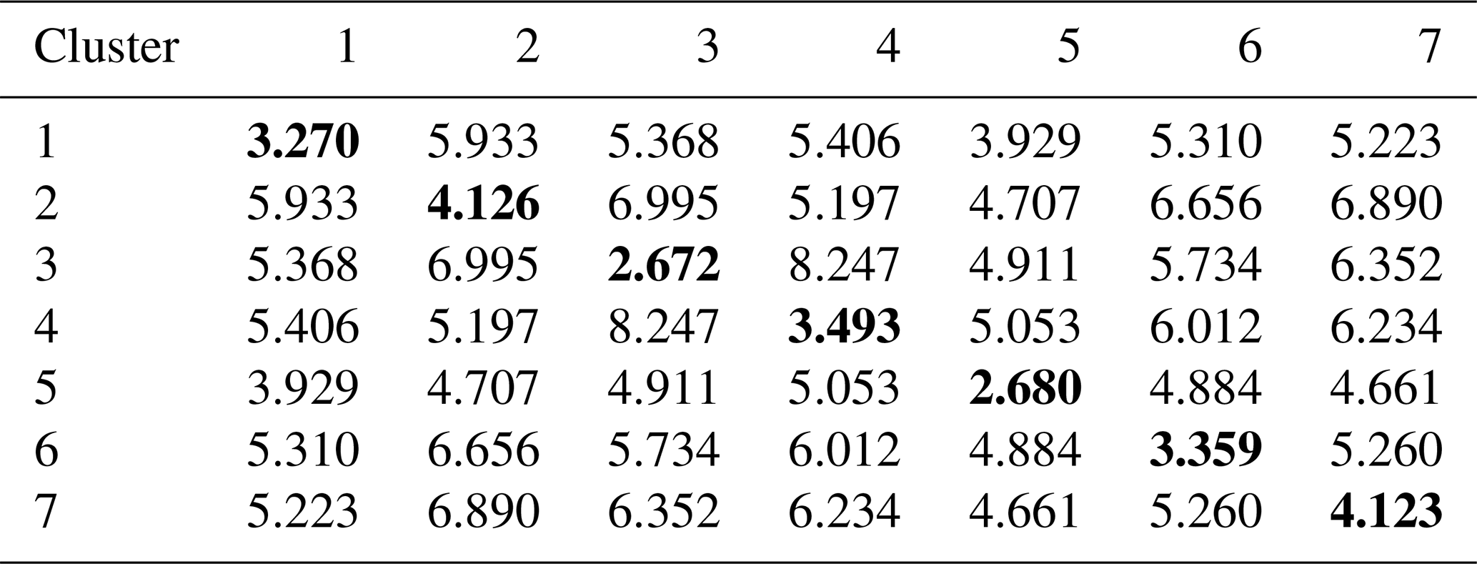
Using the unsupervised learning framework described in Sect. 2.2 and 2.3, the 75 BSRN stations are grouped into seven distinct regimes. Figure 5 shows a heatmap of pairwise Euclidean distances (denoted as Ward distance, “WD”) among the PCA-transformed station features, using principal components that explain ≥ 90 % of the total variance. The color gradient represents distance magnitude, with darker shades indicating higher multivariate similarity. Notably, the diagonal blocks are much darker than the off-diagonal regions, indicating high intra-cluster cohesion and low inter-cluster similarity and thus confirming the effectiveness of the hierarchical clustering. This result is further quantified in Table 2, which displays the mean within-cluster and inter-cluster distances in the form of a 7×7 matrix. In Fig. 5, Dendrograms along the top and left margins illustrate the nested grouping structure produced by Ward's minimum-variance method. Adjacent discrete color blocks mark the final regime assignments, partitioned according to the optimal cluster count identified by silhouette analysis. This robust regionalization provides the basis for configuring regime-specific ERL tests.

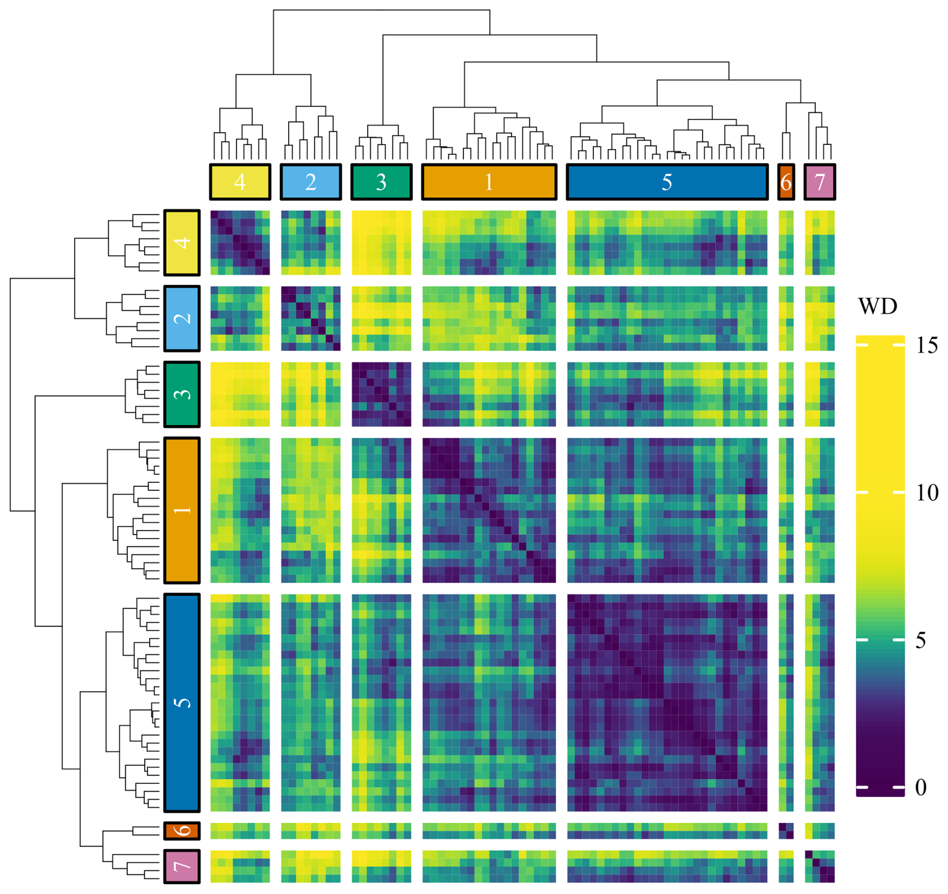
Figure 5 Heatmap and hierarchical clustering dendrogram of BSRN stations based on their radiation climatological feature space.

Table 2 Mean pairwise Euclidean distances in PCA space (first 7 PCs explaining 92.64 % variance). Whereas the mean within-cluster distances are shown as the diagonal entries, the mean inter-cluster distances are located at the off-diagonal entries. The column- and row-wise smallest distances are in bold.

To visualize the spatial distribution of the identified radiation regimes, Fig. 6 maps the BSRN stations and colors each site by its final cluster assignment. The resulting pattern shows a physically meaningful regionalization. This coherence is especially evident for the eight polar stations, which form a distinct, unified cluster due to their shared extreme annual irradiance cycles (i.e., polar day and night). In addition, geographically distant stations exposed to similar atmospheric conditions are consistently assigned to the same regime, as illustrated by the arid stations at Desert Rock (DRA) in the United States and Alice Springs (ASP) in Australia. This agreement further supports the physical relevance of the extracted distributional features. Considering both the spatial organization and the intrinsic properties of these features, the seven regimes can be interpreted as distinct global climatological zones. Table 3 summarizes the regimes, including their abbreviations, representative atmosphere/surface conditions, and defining radiation traits. A detailed discussion of each regime's physical drivers and climatological context is provided below.

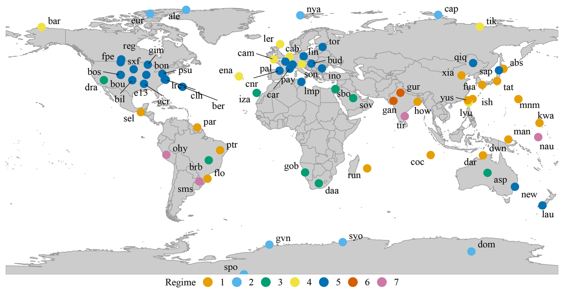
Figure 6 Geographical distribution of the BSRN stations utilized in this study, alongside their identified radiation climatic regimes.

Table 3 Seven radiation climatic regimes and their dominant characteristics.

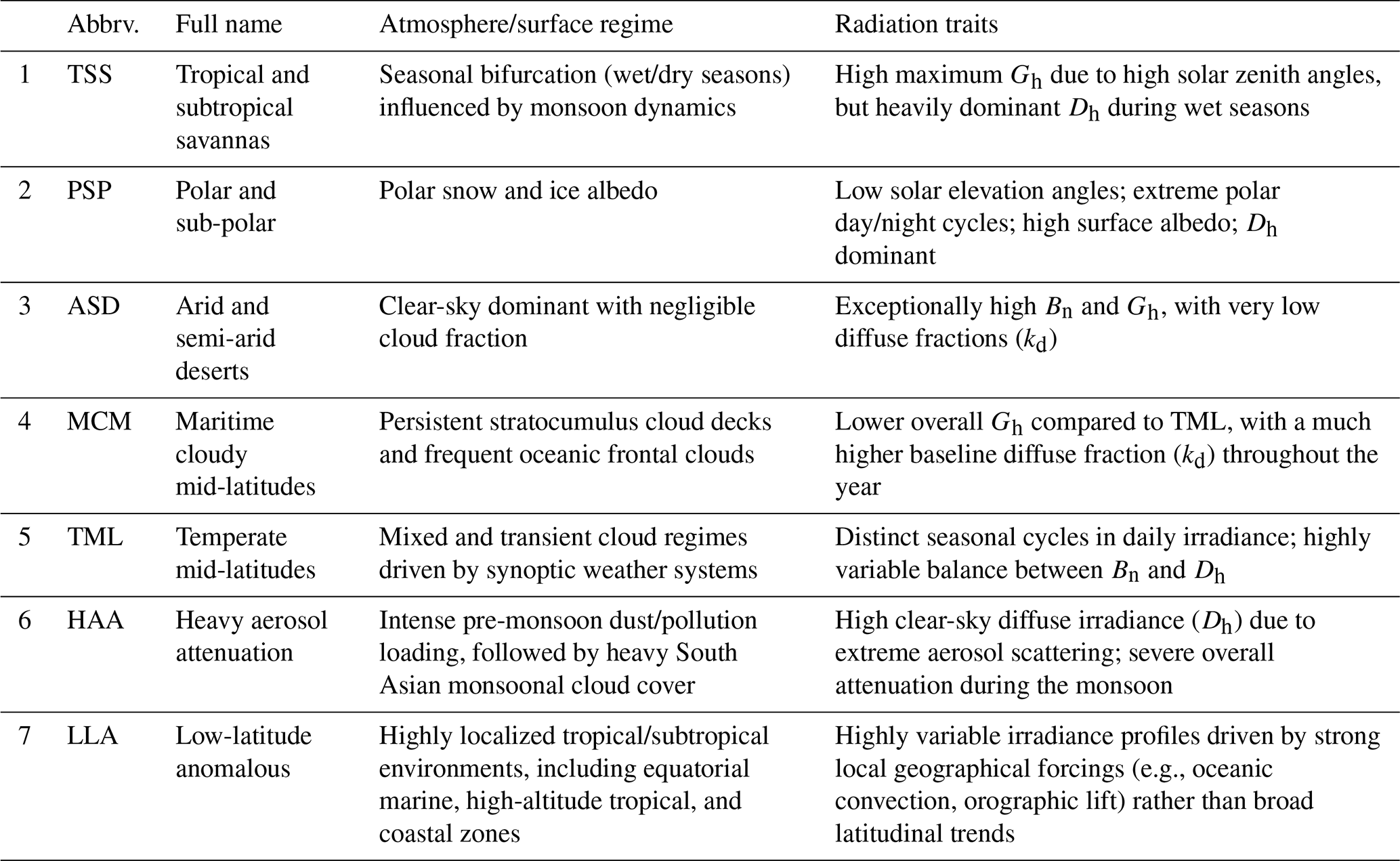
Regime 1 (tropical and subtropical savannas, TSS) comprises 18 stations with a mean absolute latitude of 20.8° and primarily represents global savanna and monsoon belts located between equatorial rainforests and subtropical deserts. The defining atmospheric feature of this regime is a pronounced wet–dry seasonal bifurcation driven by migration of the intertropical convergence zone and associated monsoon dynamics. Because these stations are at low latitudes, they maintain high solar elevation angles throughout the year, yielding exceptionally high theoretical maxima for G_h. However, the surface radiation budget shows strong seasonal variability. During the dry season, stable subsiding air linked to subtropical high-pressure systems allows extended periods of intense, largely unattenuated B_n. By contrast, wet-season onset brings deep convection and heavy precipitation, shifting the radiative balance so that D_h becomes dominant because of enhanced cloud scattering. Visual evidence and additional discussion are provided in Fig. A1 in Appendix A.

Regime 2 (polar and sub-polar, PSP) includes eight stations in extreme high-latitude environments, with a mean absolute latitude of 78.2°. This cluster is rooted in polar and sub-polar regions characterized by cold, dry air masses and persistent snow/ice cover. The key physical control is the extreme annual irradiance cycle – polar day and polar night – which keeps solar elevation angles low even during summer (Fig. A2 in Appendix A). As a result, the surface radiation budget is strongly modulated by the high albedo of frozen surfaces. Although B_n is strongly suppressed by long atmospheric optical paths and low sun angles, D_h often dominates the radiation profile. This dominance is further reinforced by multiple scattering between the reflective surface and frequent boundary-layer ice crystals or polar stratiform clouds. It should be noted that although BAR and TIK are high-latitude Arctic stations, they are assigned to another cluster because the clustering is based on multivariate features, not on latitude alone. In fact, BAR and TIK exhibit a cloud-dominated, diffuse-heavy, beam-suppressed signature that aligns with Regime 4 (see below) rather than with the drier, clearer-beam polar sites in Regime 2.

Regime 3 (arid and semi-arid deserts, ASD) comprises eight stations located mainly in subtropical high-pressure zones, with a mean absolute latitude of 26.8°. This group includes geographically distant but climatologically similar arid and semi-arid environments, such as DRA and ASP. Atmospheric conditions are controlled by persistent subsidence from the descending branches of the Hadley circulation. This large-scale subsidence maintains stable, dry air masses, minimal precipitation, and predominantly clear skies throughout the year (Fig. A3 in Appendix A). As a result, the radiation profile shows weak cloud attenuation and low atmospheric moisture. These factors produce high atmospheric transmittance, yielding consistently high B_n and G_h and very low diffuse fractions. The statistical prevalence of clear-sky days makes ASD one of the most stable and radiatively intense regimes in the surface solar radiation budget.

Regime 4 (maritime cloudy mid-latitudes, MCM) consists of eight stations across mid-to-high latitudes, with a mean absolute latitude of 51.7°. These maritime and coastal environments are strongly influenced by oceanic moisture transport and frequent subpolar low-pressure passages. Consequently, atmospheric conditions are dominated by persistent marine stratocumulus and extensive frontal cloud cover. This near-continuous cloudiness efficiently scatters incoming solar radiation, producing a substantially higher baseline diffuse fraction than in continental regions at similar latitudes (Fig. A4 in Appendix A). Although seasonal cycles in daily irradiance remain evident, persistent attenuation lowers overall G_h and strongly suppresses B_n, making D_h a defining and consistently important component of the local surface radiation budget.

Regime 5 (temperate mid-latitudes, TML) is the largest cluster in the BSRN dataset, containing 27 stations with a mean absolute latitude of 42.7°. Its broad distribution places these sites in the temperate mid-latitudes, where the Westerlies and frequent synoptic weather systems dominate atmospheric variability. Cloud and surface conditions are therefore highly transient, alternating between clear-sky anticyclonic periods and overcast conditions linked to passing cold and warm fronts. The TML radiation profile is characterized by a clear seasonal cycle in daily irradiance superimposed on strong day-to-day variability. Although summer solar elevations permit substantial G_h, the relative contributions of B_n and D_h shift markedly with synoptic state, making TML one of the most dynamically variable regimes in terms of short-term surface radiation behavior. Additional details are shown in Fig. A5 in Appendix A.

Regime 6 (heavy aerosol attenuation, HAA) is a highly specialized cluster containing only two stations, Gandhinagar (GAN) and Gurgaon (GUR), both in the Indian subcontinent. Unlike regimes shaped mainly by broad latitudinal gradients or synoptic variability, this local environment is defined by exceptionally high aerosol optical depth from severe anthropogenic pollution and pre-monsoon dust loading. As a result, even under nominally clear skies, strong atmospheric scattering produces an unusually high baseline D_h and pronounced attenuation of B_n (Fig. A6 in Appendix A). During summer, this aerosol-driven attenuation is further intensified by the arrival of the South Asian monsoon, which brings persistent cloud cover and deep convection that strongly suppress G_h. The algorithm's separation of these two stations into an independent regime – using radiation observations alone and without explicit aerosol inputs – demonstrates that the extracted climatological features robustly capture extreme scattering and attenuation processes.

Regime 7 (low-latitude anomalous, LLA) consists of a small, diverse cluster of four stations – Nauru Island (NAU), Observatory of Huancayo (OHY), São Martinho da Serra (SMS), and Tiruvallur (TIR) – representing highly localized tropical and subtropical microclimates. Unlike broader zonally organized regimes, this group is controlled by strong site-specific geographic forcings rather than latitude alone (see Fig. A7 in Appendix A). For example, grouping an equatorial marine site near sea level (NAU, 7 m) with a high-altitude Andean station (OHY, 3314 m) highlights the algorithm's sensitivity to anomalous radiation signatures. Atmospheric conditions at these sites are shaped by localized processes, such as persistent deep oceanic convection or strong orographic lifting, which produce highly variable insolation profiles. Their surface radiation budgets therefore deviate from typical low-latitude behavior, with large and irregular shifts between clear-sky B_n and strongly attenuated D_h. Identification of this anomalous regime further supports the need for a data-driven regionalization framework.

Before we move forward to discuss the configuration results, it should be noted that the seven radiation regimes are identified unsupervised from the BSRN data. Once this classification is fixed, it can be applied to new stations or locations as a supervised assignment step: extract the same features from 1 min G_h, D_h, and B_n, standardize and project them into the PCA space, and assign the site to the nearest regime. In the future, the same unsupervised classification framework could be extended to satellite-derived irradiance, enabling a gridded global regime map and spatially varying QC limits; this extension is not discussed further in this work.

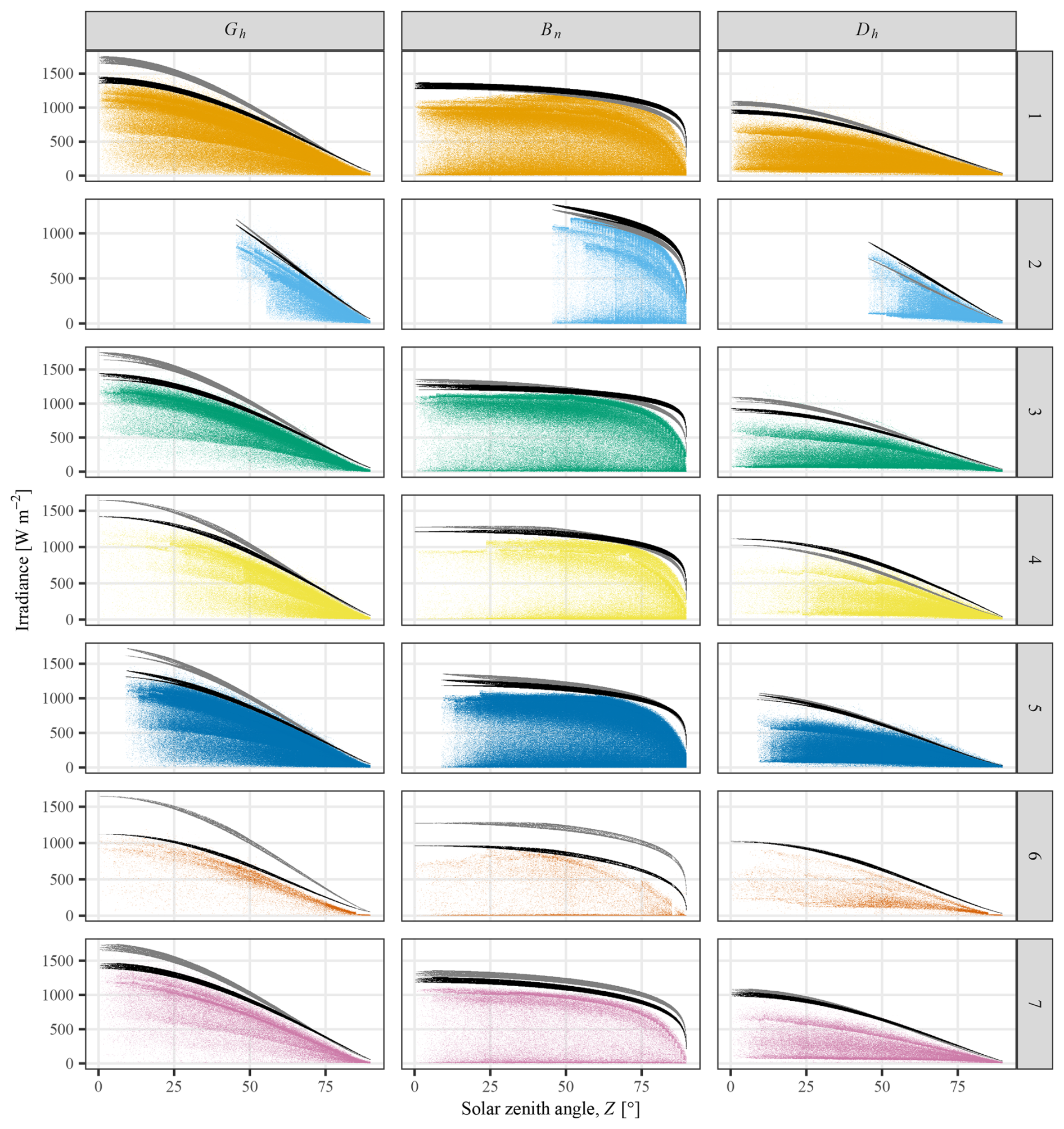
Figure 7 ERL tests for G_h, B_n, and D_h across seven radiation regimes. The configured and standard upper bounds correspond to the black and gray “eyebrows” in the figure, respectively.

3.2 Configuration result analysis

Optimization of regime-specific climatological limits is performed using a multi-stage data-driven framework designed to separate physically plausible upper boundaries from meteorological noise. To handle the large volume of 1 min observations while targeting theoretical upper limits, we adopt a stratified sampling strategy. The dataset is first partitioned into 1° zenith-angle bins. Within each bin, the top 5 % of irradiance values for G_h, B_n, and D_h are extracted to represent the upper envelope. To preserve typical observational states and the broader distributional structure, this envelope-focused sample is supplemented with a 10 % random sample from each bin. An iForest – configured with 100 trees in a three-dimensional feature space comprising k_t, k_d, and k_b – is deployed to assign binary classifications to each data point using a kernel-density-estimated threshold. Structural limit curves, defined by $I=a{E}_{\mathrm{0}n}{\mathit{\mu }}_{\mathrm{0}}^b+\text{const}$, are fitted to these boundaries. The L-BFGS-B optimizer is used to estimate coefficients (a,b) by maximizing the F₁ score relative to the iForest labels. The initial values for both a and b, for each component and cluster, are set to 1; the algorithm converged for all cases.

Table 4 reports the optimized coefficients and corresponding F₁ scores for all seven radiation regimes. The consistent F₁ range of 0.98–0.99 across all three components ($F_{\mathrm{1},G},F_{\mathrm{1},B},F_{\mathrm{1},D}$) provides strong quantitative evidence that optimization successfully identifies the physical boundaries isolated by the unsupervised framework. Coefficient patterns also reflect distinct physical regimes. For G_h, the amplitude factor a_G remains relatively constrained (0.81–1.10), and the zenith-response exponent b_G is stable across clusters (1.05–1.25).

Table 4 Optimized parameters for the proposed QC limits across seven radiation climatic regimes. Constant terms are fixed at c_G=50, c_B=10, and c_D=30 W m⁻².

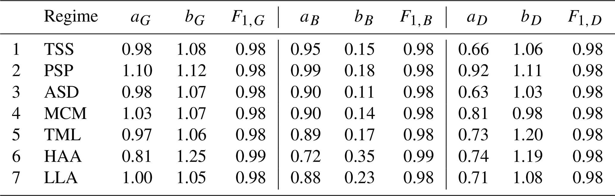
The B_n coefficients further reflect atmospheric attenuation effects. Most pristine and temperate regimes have a_B values in the range 0.88–0.99, whereas Regime 6 drops markedly to a_B=0.72. This quantitatively captures the large beam-radiation suppression associated with high aerosol loading over the Indo-Gangetic Plain and demonstrates the method's ability to regionalize anthropogenic attenuation. In addition, b_B is systematically lower than b_G (0.11–0.35), consistent with the stronger zenith-angle sensitivity and faster decay of direct-beam irradiance at high solar zenith angles.

Finally, D_h limits show substantial regional variability, especially in the amplitude factor a_D, which controls the theoretical upper envelope for diffuse scattering. The optimized results indicate that the upper boundary of diffuse irradiance is strongly regime dependent. For example, the stable, clear-sky conditions in Regime 3 yield a comparatively low envelope (a_D=0.63). In contrast, strong-scattering environments require much higher limits to avoid falsely flagging valid data; Regime 2 is a clear example, with a_D=0.92 and a steeper zenith-response exponent b_D=1.11. These values quantitatively represent diffuse dominance under high-albedo, multiple-scattering conditions over polar snow and ice. Overall, the coefficient contrasts confirm that a single global QC limit cannot represent the diverse scattering physics across global radiation climates.

3.3 Quality control result comparison

To evaluate the performance of the proposed climatological limits relative to the baseline BSRN ERL limits, QC outcomes are compared across all identified radiation regimes. Figure 7 presents a 7×3 matrix of scatter plots showing measured irradiance components versus solar zenith angle for all seven regimes. The superimposed “eyebrows” indicate the boundary differences between the static ERL and the configured climatological limits. For G_h, ERL thresholds are consistently broader than the proposed limits in all regimes, confirming the known tendency of ERL to be overly permissive. For B_n, the two limit sets are generally similar, except in Regime 6, where the configured limits are markedly more restrictive and better adapted to high-aerosol, low-beam conditions. For D_h, the comparison is regime dependent: ERL limits can be higher, comparable, or lower than the configured limits, which motivates further quantitative analysis.

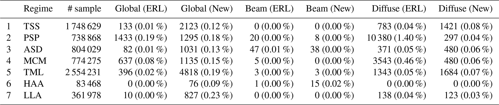
Table 5 translates these visual differences into operational QC impacts by comparing rejection rates under the baseline ERL and the proposed climatological limits. Under standard ERL settings, QC is generally too permissive across most regions, with near-zero rejection rates in many regimes. By reducing the excess buffer above the observed physical scatter, the proposed limits tighten constraints and raise rejection rates to more informative ranges. The value of regionalization is especially clear in two regimes: polar/sub-polar (PSP) and heavy aerosol attenuation (HAA). In PSP, ERL is overly strict for the diffuse component, flagging 1.40 % (10 380 points) of D_h samples. The customized limit relaxes this boundary and reduces the D_h rejection rate to 0.04 %. In contrast, in the polluted HAA regime, global ERL fails to provide meaningful upper-bound control, rejecting none of the G_h and D_h samples because aerosol-suppressed observations remain below the ERL ceiling. The clustered limits correct this blind spot, restoring sensitivity and increasing the G_h and D_h rejection rates to 0.09 % and 0.02 %, respectively.

Table 5 Component-wise rejection counts and rates. The absolute numbers are on top, and percentages bottom.

To further explain why ERL frequently discards data in Regime 2, we conduct a false-positive analysis for the Alert (ALE) station in the Lincoln Sea (Fig. 8). An automated scan identifies a continuous 24 h period (30 May 2010) with an exceptionally high ERL rejection rate but excellent radiometric closure ($G_{\mathrm{h}}\approx D_{\mathrm{h}}+{\mathit{\mu }}_{\mathrm{0}}{B}_{\mathrm{n}}$). On that day, the static ERL test flags 1147 of 1440 points as erroneous. However, physical validation via the closure equation shows a mean closure error of only 1.10 %, with a maximum error of 3.78 % over the full diurnal cycle. This near-perfect agreement indicates that the sensors were operating correctly and that the elevated diffuse scattering was a real atmospheric signal rather than an instrumental artifact. Thus, while standard ERL fails to accommodate intense polar scattering and causes substantial data loss, the proposed climatological limits correctly envelop these valid enhancements, reducing false positives while retaining physically justified upper bounds.

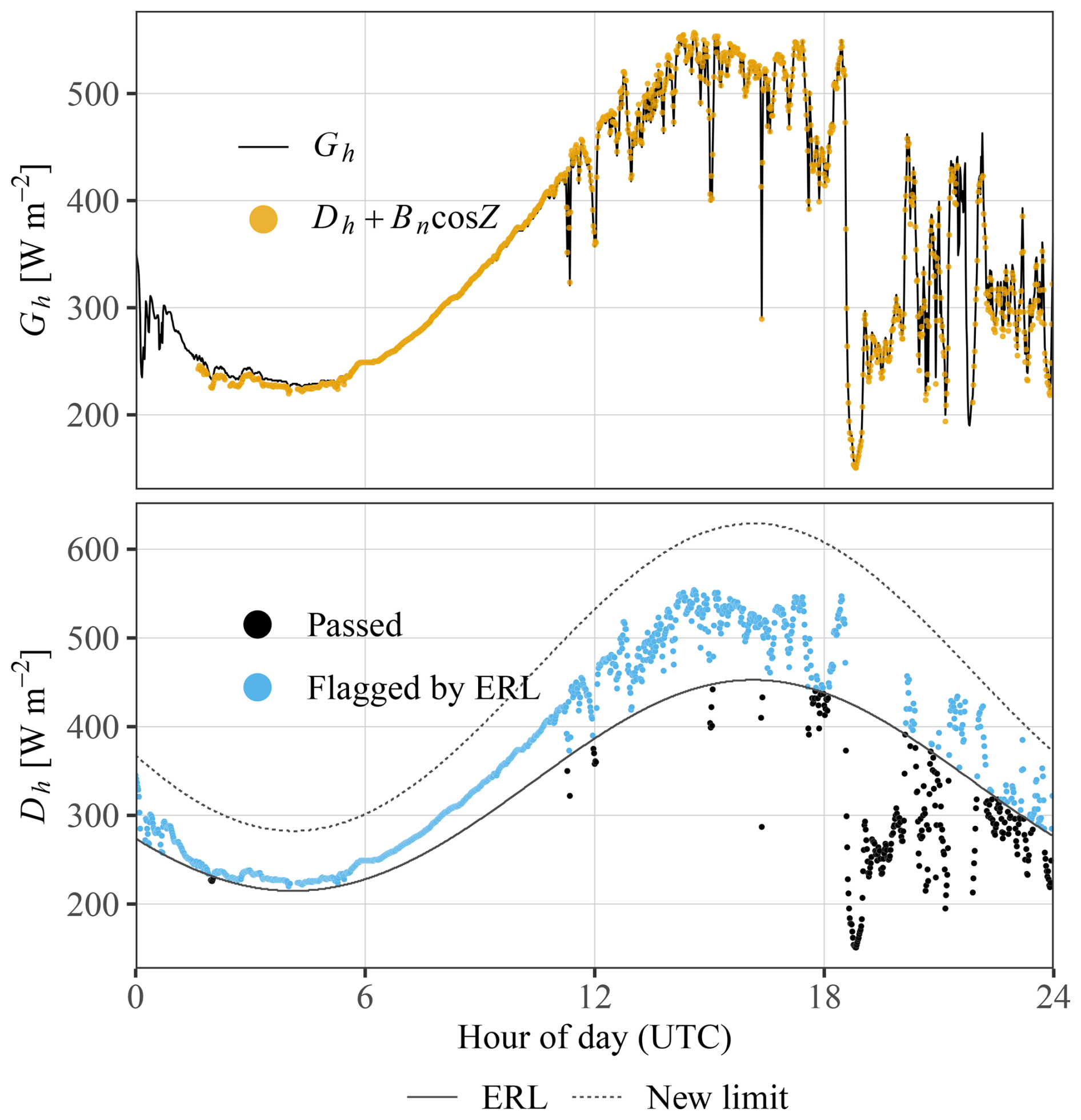
Figure 8 False-positive analysis of the ERL test during a 24 h period in Regime 2 (Polar/Sub-Polar). (Top) Radiometric closure (1.10 % mean error) confirms the physical validity of the measurements. (Bottom) The ERL test incorrectly flags 1147 of 1440 valid D_h observations, whereas the proposed clustered limits successfully retain them.

4 Conclusions

Quality control (QC) of ground-based solar radiation measurements is fundamental for maintaining the integrity of surface energy balance and climatological studies. However, the widely used extremely rare limit (ERL) test is often overly conservative and can fail to isolate subtle instrumental or environmental anomalies. To improve QC tightness and sensitivity, this study presents a data-driven framework for configuring regime-specific climatological limits. Using a multidimensional unsupervised learning approach – combining principal component analysis and hierarchical clustering – BSRN stations were grouped into seven distinct radiation climatic regimes based on radiation climatological features.

For each regime, optimal coefficients for climatological limit curves were determined through machine-learning-based optimization. The empirical parameters were optimized within bounded constraints using the L-BFGS-B algorithm. The objective function explicitly maximized the F₁ score by benchmarking climatological-limit classifications against reference inlier–outlier labels generated by an iForest model.

Validation shows that the resulting parameter sets are more robust than the traditional ERL test, providing tighter envelopes around observations and improving QC sensitivity. The regime-specific limits adapt to local atmospheric conditions: they relax overly strict diffuse constraints in the polar and sub-polar (PSP) regime to reduce false-positive rejections linked to polar snow-albedo effects, while restoring upper-bound sensitivity in the heavily polluted HAA regime. The spatial variability of fitted parameters reflects regional differences in solar elevation, cloud regimes, and atmospheric transmissivity, supporting the physical consistency of the proposed radiation climate classification.

Overall, the proposed optimization framework mitigates the conservativeness and regional inconsistency of conventional empirical thresholds and provides a scalable, automated pathway for regionalized QC. It establishes a methodological basis for developing a unified global radiation data quality-control system. It is noted that the same modeling philosophy can be applied to other QC tests, such as the closure test or the tracker-off test. Future work will incorporate long-term meteorological reanalyses and radiative-transfer modeling to assess temporal variability and seasonal adaptability of the configured climatological limits. Additionally, incorporating auxiliary data that reflects site climatology, such as surface albedo or longwave radiation, could further enhance the robustness of the radiation climate classification. As climate classification remains an ongoing task, this work is intended to serve as a preliminary framework for future developments in the field.

Appendix A: Physical characterization of the derived radiation regimes

Figure A1 supports the characterization of Regime 1 (TSS) by illustrating its seasonal bifurcation using daily maximum GHI data from the Darwin (DAR) station in 2014. The region's geographical setting yields a high and relatively stable theoretical irradiance ceiling, with the McClear clear-sky model (orange line) remaining near or above 1000 W m⁻². In contrast, measured daily maximum G_h values (blue points defining the gray envelope) show strong seasonal variability. During the dry season (approximately May–September), observed G_h closely follows the clear-sky limit, consistent with largely cloud-free and stable atmospheric conditions. During the monsoon season (approximately December–March), driven by intertropical convergence zone dynamics, measured maxima diverge sharply from the McClear envelope because of strong and highly variable cloud attenuation. This contrast – a smooth theoretical maximum repeatedly interrupted by deep wet-season attenuation – illustrates the regime-specific physical behavior that must be accounted for when configuring QC limits.

Figure A2 supports the characterization of Regime 2 (PSP) by mapping its extreme diurnal constraints using theoretical clear-sky GHI simulations for the Ny-Ålesund (NYA) station in 2021. The heatmap shows irradiance intensity by day of year (x-axis) and hour of day (y-axis), with white dashed (α=0°) and solid (α>0° at 10° intervals) contours indicating solar elevation angle (α). Rather than stochastic daily variability, the figure displays a pronounced “hourglass” geometry governed by high-latitude solar geometry. Dark regions at the beginning and end of the annual cycle represent polar night, when irradiance remains 0 W m⁻² throughout the day because α≤0°. In contrast, the central summer period (approximately May–August) forms a continuous vertical irradiance band, indicating polar day. However, even during continuous daylight, the maximum solar elevation remains below about 35°, as shown by the contour structure. Accordingly, peak theoretical irradiance remains substantially lower than at lower latitudes. This behavior highlights why Regime 2 requires dedicated QC boundaries that differ fundamentally from mid-latitude frameworks.

Figure A1 Visual evidence supporting the discussion of Regime 1 (TSS) in Section 3.1.

Figure A2 Visual evidence supporting the discussion of Regime 2 (PSP) in Sect. 3.1.

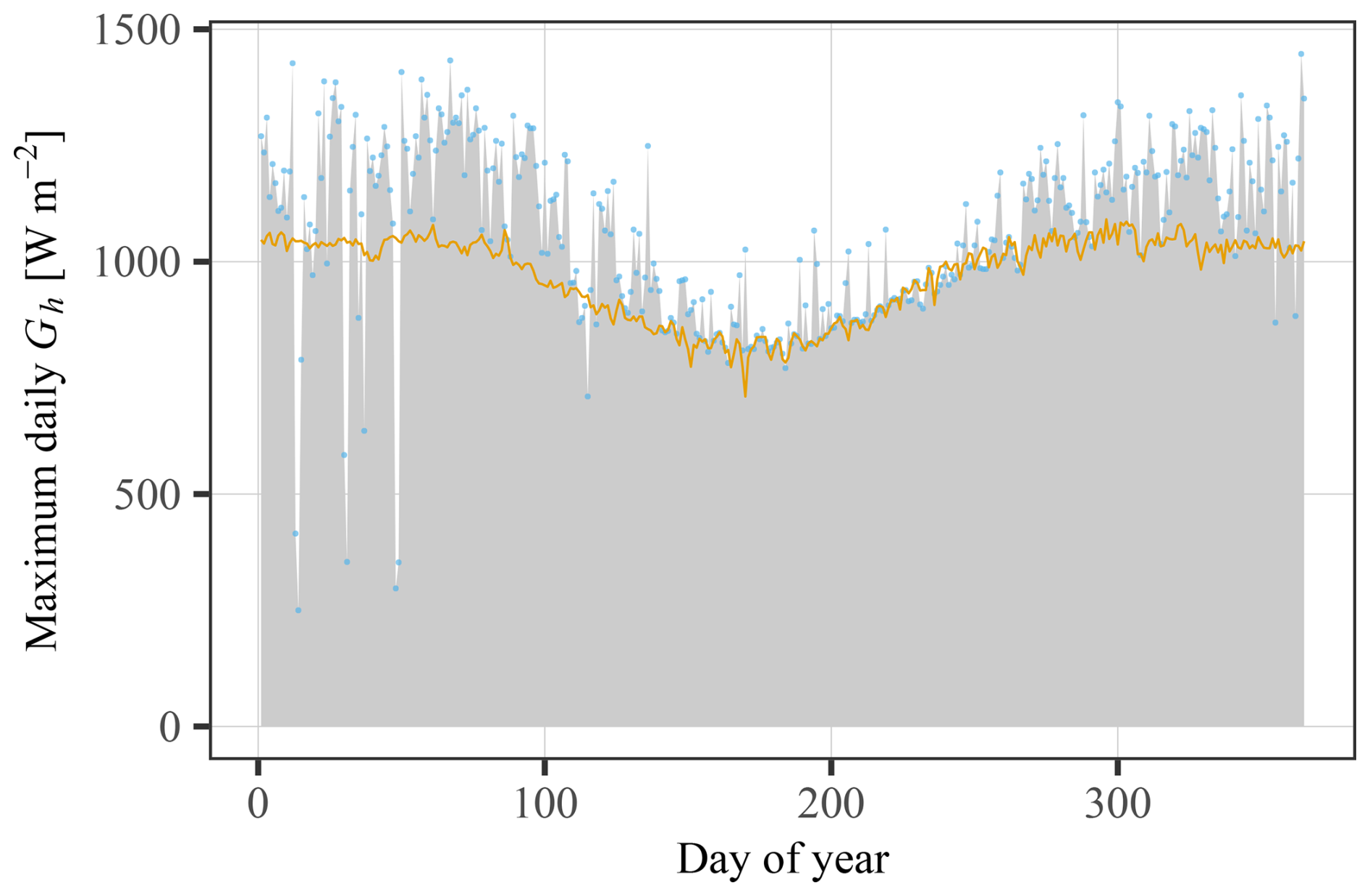
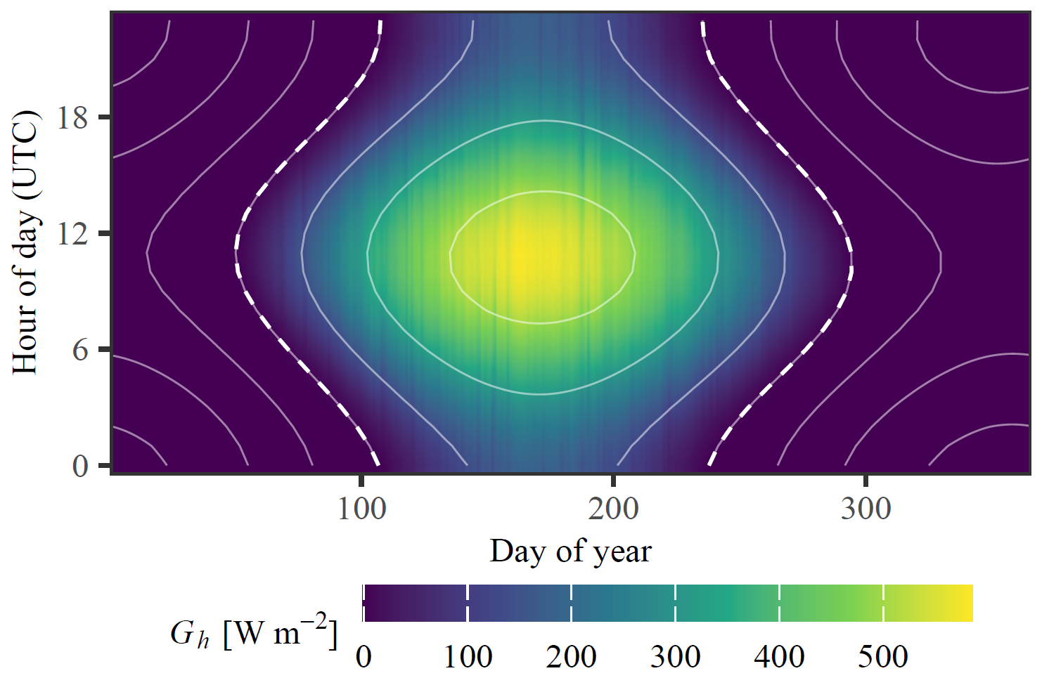
Figure A3 corroborates the environmental constraints of Regime 3 (ASD) by showing monthly probability-density distributions of the 1 min clear-sky index (κ) at the Desert Rock (DRA) station in 2021. Consistent with persistent subtropical high-pressure systems, these distributions translate the region's dry and cloud-sparse conditions into a stable statistical signature. Violin plots show that, across all months, most instantaneous κ values cluster near the dashed reference line at κ=1.0, corresponding to near-ideal clear-sky conditions with minimal cloud attenuation. Unlike temperate or monsoon climates, which often show bimodal κ distributions from frequent cloud transitions, Regime 3 exhibits limited cloud-driven variability. The narrow spread across both winter and summer confirms that radiative transmission in this regime is largely unimpeded by transient clouds and moisture variations.

Figure A3 Visual evidence supporting the discussion of Regime 3 (ASD) in Sect. 3.1.

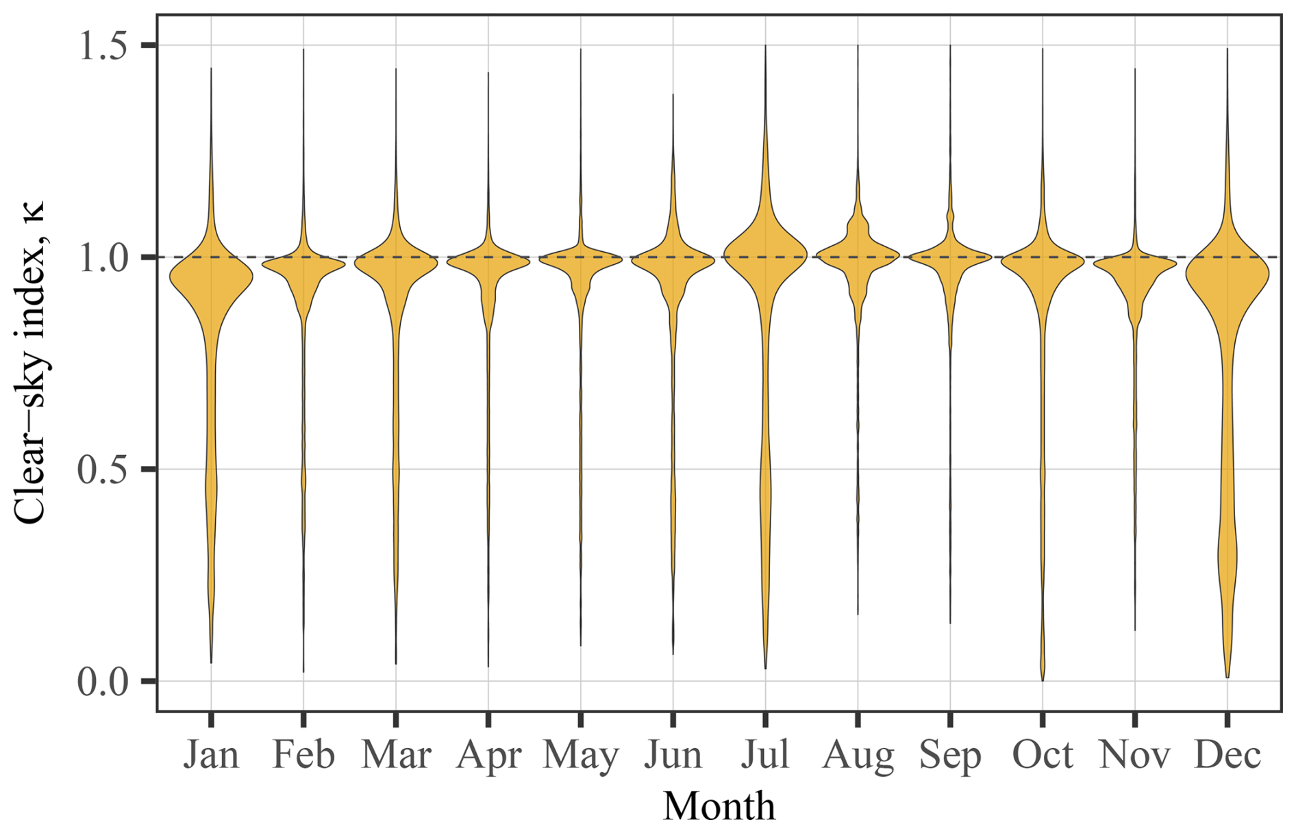
Figure A4 quantifies the persistent radiative attenuation in Regime 4 (MCM) using kernel-density distributions of diffuse fraction ($k=D_{\mathrm{h}}/G_{\mathrm{h}}$). The 1 min k distribution from Lerwick, UK (Regime 4), is compared with Fort Peck, USA (Regime 5), with both sites near 55° N. As discussed in the main text, Regime 4 is strongly influenced by persistent maritime stratocumulus and frontal cloud systems. This is reflected in a clear contrast between the two distributions. The continental site shows a pronounced clear-sky peak near k≈0.15, indicating frequent direct-beam-dominant conditions. In contrast, the marine distribution lacks a comparable clear-sky peak and instead shifts strongly toward high k values approaching 1.0. This right-skewed pattern indicates sustained atmospheric scattering and confirms the diffuse-dominant nature of Regime 4.

Figure A4 Visual evidence supporting the discussion of Regime 4 (MCM) in Sect. 3.1.

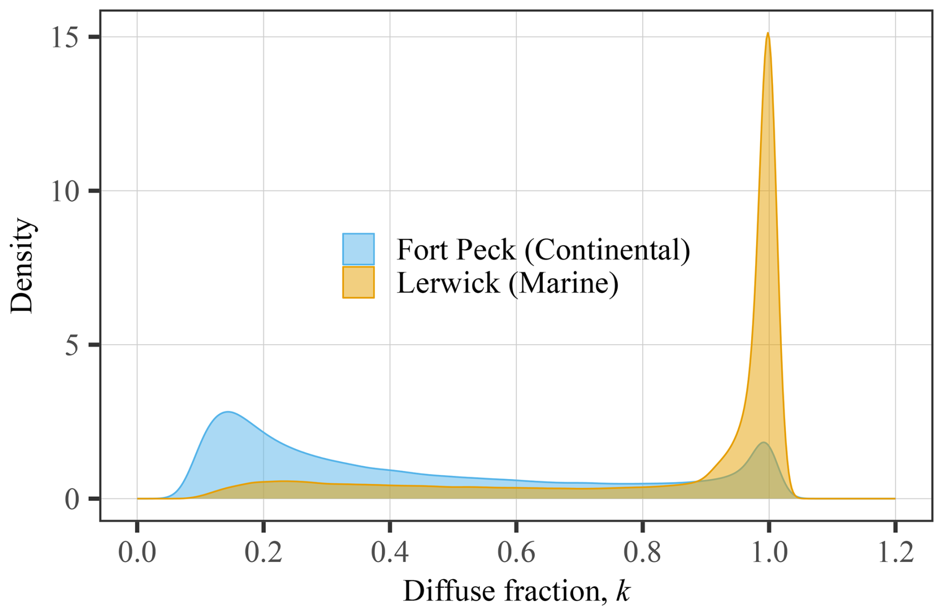
Figure A5 characterizes the radiative variability of Regime 5 (TML) using daily mean B_n and D_h time series from Payerne, Switzerland (PAY), in 2021. Under strong influence from the Westerlies, this regime is shaped by frequent synoptic weather transitions. The figure illustrates the interaction between seasonal solar forcing and short-term meteorological variability. The upper envelope of B_n follows a clear seasonal cycle controlled by mid-latitude solar elevation, while day-to-day variability remains strong. Anticyclonic periods produce clusters of high B_n values near the seasonal upper boundary, but these are repeatedly interrupted by passing fronts that sharply reduce B_n. During these frontal episodes, D_h increases rapidly, indicating fast transitions from beam-dominant to diffuse-dominant conditions. This high-frequency alternation confirms Regime 5 as one of the most dynamically variable radiation climates.

Figure A5 Visual evidence supporting the discussion of Regime 5 (TML) in Sect. 3.1.

Figure A6 Visual evidence supporting the discussion of Regime 6 (HAA) in Sect. 3.1.

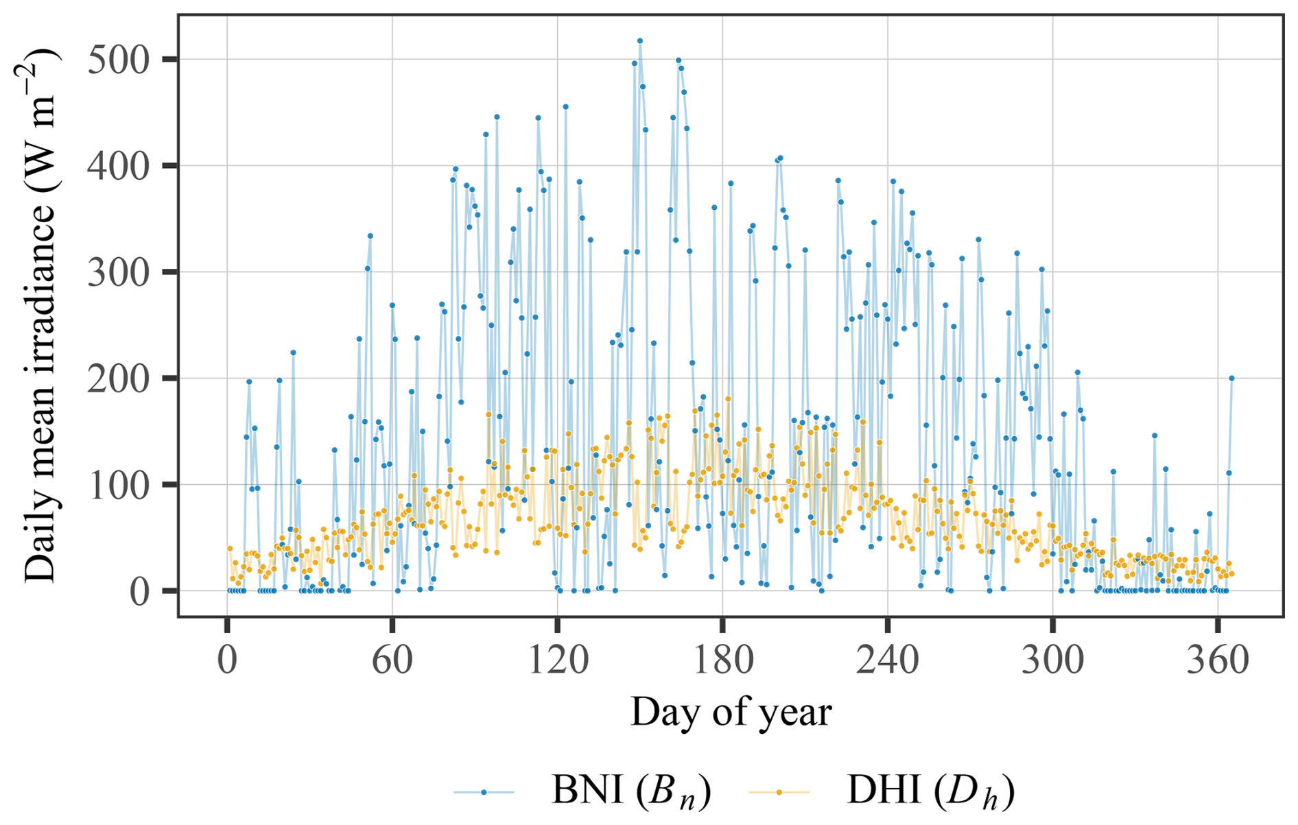
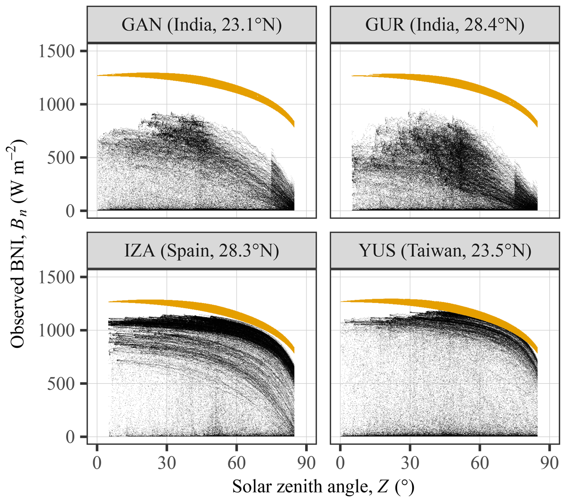
Figure A6 highlights the persistent attenuation in Regime 6 (HAA) by comparing observed B_n versus solar zenith angle for polluted Indian stations (GAN and GUR) and latitudinally comparable high-altitude clean reference sites, namely, Yushan and Izaña (YUS and IZA). This pairing keeps astronomical forcing broadly comparable and isolates atmospheric-composition effects. (It is noted that the anomalous sampling of low-sun observations and the sharp cut-off at Z=75° observed at GAN and GUR are not reflective of the underlying radiation regime, but are artifacts of the data QC before BSRN archiving, where the low-sun observations are not subjected to filtering.) In the figure, the standard ERL upper bound for B_n is shown as the orange dotted “eyebrow.” The two reference stations produce B_n values that approach this ERL boundary. By contrast, Regime 6 stations in the Indo-Gangetic Plain show strong beam suppression across nearly all zenith angles. Even under nominally clear conditions, observations remain well below the ERL ceiling. This persistent “ceiling gap” is consistent with high aerosol optical depth from anthropogenic pollution and dust loading, acting as a continuous atmospheric filter on surface beam irradiance.

Figure A7 Visual evidence supporting the discussion of Regime 7 (LLA) in Sect. 3.1.

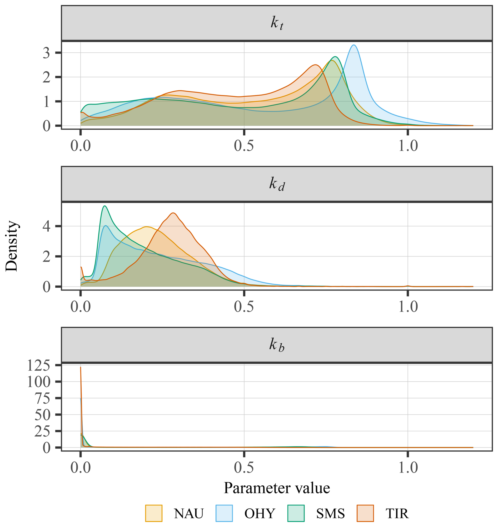
Figure A7 provides empirical support for the clustering algorithm's ability to move beyond simple geographic or latitudinal grouping by showing overlaid probability-density distributions of clearness index (k_t), diffuse transmittance (k_d), and beam transmittance (k_b) for the four Regime 7 (LLA) stations. Although these stations are geographically diverse, their distributions are statistically similar, with comparable modes and spread. This shared radiative signature persists despite large differences in altitude and local climatology, indicating that the algorithm captures structural similarities in surface radiation behavior rather than location alone. Grouping these anomalous microclimates into one cohesive regime supports the need for data-driven regionalization and identifies a class that is physically distinct from typical low-latitude regimes while statistically unified in radiative response.